Electrical Consumption Profile Clusterization: Spanish Castilla y León Regional Health Services Building Stock as a Case Study

Abstract

Health Services building stock is usually the top energy consumer in the Administrative sector, by a considerable margin. Therefore, energy consumption supervision, prediction, and improvement should be carried out for this group in a preferential manner. Most prior studies in this field have characterized the energy consumption of buildings based on complex simulations, which tend to be limited by modelisation restrictions and assumptions. In this paper, an improved method for the clusterization of buildings based on their electrical energy consumption is proposed and, then, reference profiles are determined by examining the variation of energy consumption over the typical yearly consumption period. The temporary variation has been analyzed by evaluating the temporary evolution of the area consumption index through data mining and statistical clusterization techniques. The proposed methodology has been applied to building stock of the Health Services in the Castilla y León region in Spain, based on three years of historical monthly electrical energy consumption data for over 250 buildings. This building stock consists of hospitals, health centers (with and without emergency services) and a miscellaneous set of administrative and residential buildings. Results reveal five distinct electrical consumption profiles that have been associated with five reference buildings, permitting significant improvement in the demand estimation as compared to merely using the classical energy consumption indicators.

1. Introduction

In order to comply with European Union (EU) perspectives on energy generation and consumption by EU members for the 2030 and 2050 horizons, a significant increase in the penetration of renewable energy sources (RES) and a reduction of energy needs, through energy savings and efficiency policies, are mandatory. Both approaches are especially relevant in the transport and buildings sectors, and within the latter, Public Administration building stock is of special relevance.

On the other hand, reliable energy indexes must be developed in order to supervise the evolution of the consumed energy, which is ultimately associated with greenhouse effect gas emissions. This detailed supervision intends to assist energy planners in achieving local, national, and European targets for energy savings and efficiency.

Typically, the evaluation of a building’s energetic behavior is carried out via computer simulation and the assignment of energy labels is based on the results of the same and its comparison with reference buildings. This method has been demonstrated to show a great accuracy in some specific cases [1], but considerable dispersion appears when analyzing large buildings, such as hospitals, which are usually characterized by complex air conditioning equipment and high electric energy consumptions. Moreover, most energy labeling methods do not currently consider the electric energy consumption of the building—such as thermal (heating and/or cooling)—since the building’s request is usually noticeably larger (both in magnitude and price terms) as compared to the electric energy and since those needs are vigorously associated to the level of occupation and activity. However, as the nearly Zero Energy Buildings (nZEBs) and Positive Energy Buildings (PEBs) are being deployed, energy consumption needs associated with the thermal behavior of the building are becoming increasingly lower over time and it is expected that soon, building energy needs will be mainly associated with their electric energy needs [2].

However, it may be difficult to carry out representative simulations of the electric energy needs of a building, due to their relationship with the oscillating level of activity. The recently developed “big data” and “data mining” techniques may help to treat real measurements from a large amount of buildings’ metering systems. Thus, real power demand profiles can be created from suitable data treatment, instead of using simplified power demand profiles, thus significantly improving the final modelization of the facilities [3].

In this study, the authors propose a novel method to identify and classify buildings according to their electric energy demand profile during a natural year period by applying clustering techniques. The aim of this work is to identify general classes of buildings according to their electric energy consumption and to improve not only the demand estimations, but also the aggregation of electric energy profiles of different buildings, which results truly useful for centralized energy purchasing, energy consumption monitoring by activity sectors and fast identification of abnormal consumption behaviors. Other applications of the proposed method are related to the optimization of the definition of Power Purchase Agreements (PPAs) in the public sector or the optimal introduction of the Electric Vehicle (EV), among many others [4,5,6,7]. Taking into account a proposed case study, this methodology has been applied to the health system stock of the Castilla y León region in Spain, which consists of approximately 250 buildings of different sizes and final uses.

This paper is divided into three sections. The first section includes the introduction to the topic, and the reference framework in the EU zone and a description of the building stock from the health system of the Castilla y León region, which has been used as a case study. The second section, entitled “Materials and Methods”, describes the proposed methodology and the origin of the used data. Scope and limitations of the work are also presented in this section. The next section presents and discusses the obtained results, while the final section collects the authors’ conclusions and proposals for future research in the field.

1.1. Innovations Introduced by the 2018/844/EU Directive

On 30 May 2018, EU Directive 2018/844 [8] was published, updating Directive 2010/31/EU [9] on the energy performance of buildings and Directive 2012/27/EU [10] on energy efficiency. In this document, the EU declares its commitment to developing a sustainable, competitive, secure, and decarbonized energy system, while at the same time it recalls the commitments of the Energy Union and the Energy and Climate Policy Framework for 2030. The EU Commission finds the need to provide Member States and investors a clear vision to guide their policies and investment decisions, including national milestones and actions for energy efficiency to be accomplished over the short-term (2030), mid-term (2040), and long-term (2050). Then, it is required that Member States specify the expected output of their long-term renovation strategies and monitor developments by establishing domestic progress indicators, which are subject to national conditions and developments.

In order to meet proposed goals in the energy field, the EU concludes that Member States and investors need to apply new measures, and it focusses on the need for the de-carbonization of the building stock, responsible for approximately 36% of all CO₂ emissions in the Union, as soon as possible. This conclusion is in line with those from the 2015 Paris Agreement on climate change following the 21st Conference of the Parties to the United Nations Framework Convention on Climate Change (COP 21), boosting the EU’s efforts to decarbonize its building stock.

To achieve a highly energy efficient and decarbonized building stock and to ensure that the long-term renovation strategies result in the necessary progress towards the transformation of existing buildings into nZEBs, or even PEBs, clear guidelines should be provided and, more importantly, measurable, targeted actions should be established [11,12].

Each long-term renovation strategy should be in line with applicable planning and should encompass, among other conditions: (i) an overview of the national building stock; (ii) policies and actions to target all public buildings; and (iii) an evidence-based estimate of expected energy savings and wider benefits, establishing measurable progress indicators. Moreover, databases for energy performance certificates should permit data collection on the measured or calculated energy consumption of the buildings covered, including at least the public buildings stock.

It should be noted that EU Directive 2018/844 points out the real need to determine the energy performance of a building based on its calculated or actual energy use and it shall reflect typical energy use, not only for space heating, cooling or domestic hot water, but also for lighting and other electrical technical building systems [8].

1.2. Power Consumption of the Health System in the Castilla y León Region

The Autonomous Community of Castilla y León in Spain is the sixth largest region of the country, having almost 2.5 million inhabitants in 2018 and with health services that are divided into 39 different areas including primary care, specialized health, and administrative sections. It serves the medical needs of over two million patients with 7.81 health professionals per every thousand potential patients [13].

The building stock of the health system in Castilla y León consists of different sets of buildings, which are usually classified into hospitals and health centers. The latter may also be organized into health centers with and without emergency services. Clinics, residences and administrative buildings and warehouses are the minority and they are usually classified as “others”.

Table 1. Description of electrical energy consumption of the Public Health System′s building stock in the Castilla y León region in Spain. Data source: Junta de Castilla y León.

Building Type	Inventory	Average Consumption (MWh·year−1)	Sd. Deviation (MWh·year−1)	Consumption Share (%)
Hospitals	27	107,214,549	5,873,670	82.45
Health centers with emer.	176	7,357,180	226,053	5.66
Health centers without emer.	91	7,871,277	221,585	6.05
Others	60	7,593,819	614,003	5.84
Total	354	130,036,825	6,236,986	100.00

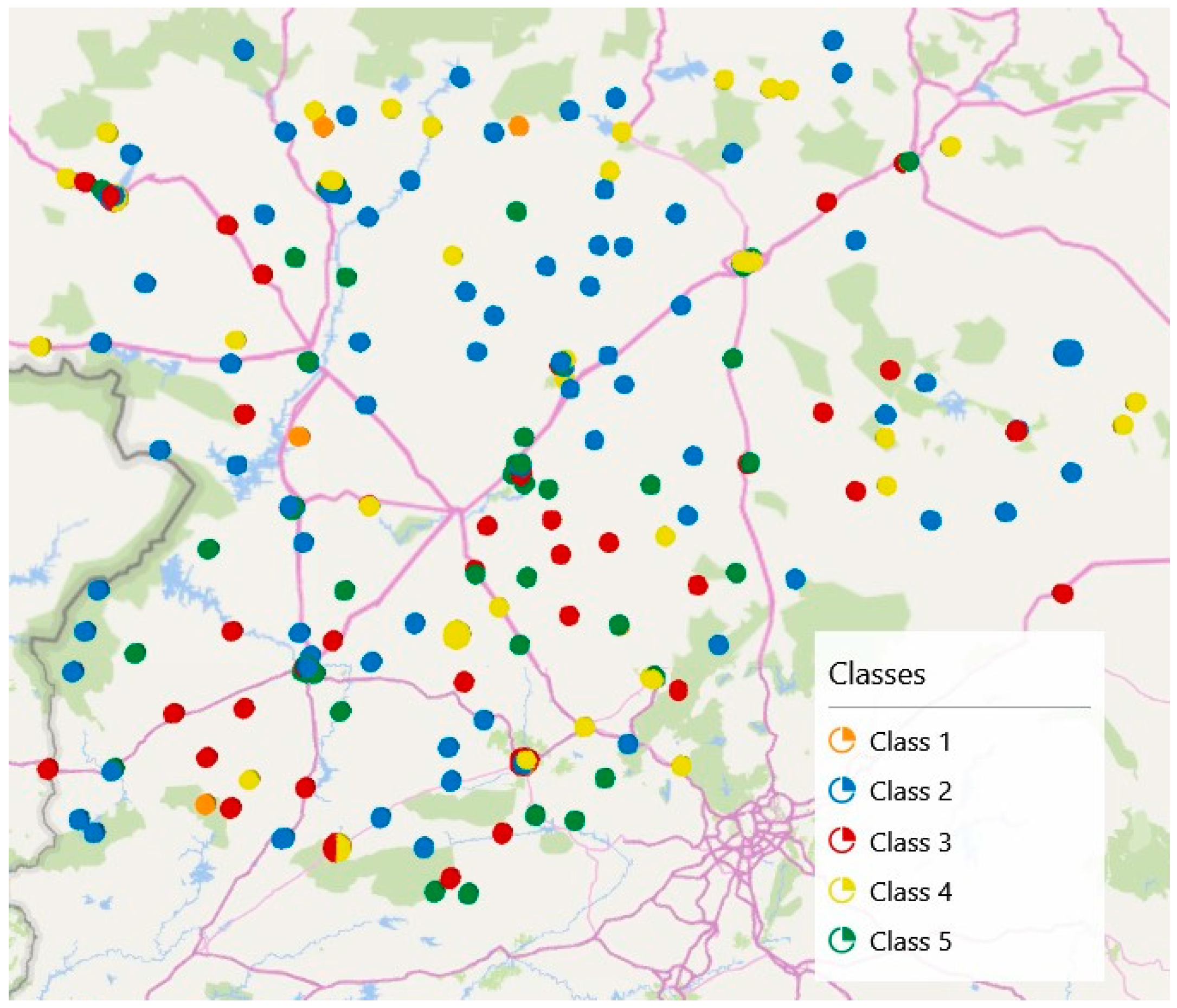
Sd. = standard. MWh = Megawatts per hour.

shows the inventory description of each category, focusing on their electrical energy needs, while Figure 1 shows their distribution. Figure 1a helps introduce the reader to the energy context, showing the geographical distribution of the average annual Area Consumption Index (ACI), while the pie chart shown in Figure 1b depicts the electrical energy consumption distribution for the described administrative categories.

It can be observed that the majority of the annual electricity consumption comes from the hospitals (almost 81% of the total). The other categories represent approximately 25 GWh·year⁻¹ of annual electric consumption. On the other hand, the variation in total electricity consumption, evaluated through the standard deviation, is relatively small on an annual basis, considering the evaluated period, which is from January 2015 to December 2017.

Finally, it should be noticed that the buildings classification provided is valid for administrative purposes, but is inefficient for an energy analysis. Thus, one of the main objectives of this paper is to show the obtained results of a new proposed method to identify reference buildings according to an energetic perspective, which may differ from a purely administrative classification.

1.3. Building Sustainability, Energy Indexes, and Annual Electric Energy Profiles

Several authors claim that over recent times, world energy consumption has increased disproportionately in relation to population growth, mainly as a result of economic development and a lack of social awareness [14]. Thus, many studies have attempted to assess the sustainability of the energy consumption at a global level, from a demand side perspective, concluding that the building industry requires more attention and more effective actions than other sectors due to its high energy consumption [15,16]. So, a growing number of countries have introduced energy-efficient strategies in their public-use buildings. Currently, energy consumption in public buildings is 40% greater than that of residential buildings and 30% of the non-residential buildings in Europe are public buildings [14]. Therefore, evaluation of building energy efficiency and energy conservation is extremely necessary [17].

Many authors have considered the intense energy consumption problem of the building sector by considering thermal consumption [17,18,19] and therefore, different solutions highlighting bioclimatic architecture strategies [20] have been proposed with great success. Bioclimatic architectural systems have demonstrated that they can effectively contribute to the reduction of energy consumption while considering potential construction solutions at both passive and active levels. These analyses have been carried out not only for residential buildings, but also for industrial ones where energy savings through the incorporation of automation techniques are difficult to afford and when there is no single directive or standardized method of estimating and validating the energy consumption process in such buildings [18].

Although thermal comfort in Northern European countries has low impact on power consumption, as they are usually satisfied by gas boilers the warmer countries face high electricity energy demands in public buildings due to air conditioning needs [19]. Furthermore, these systems are quite sensitive to slight outdoor temperature changes and climate change has forced engineers to find and design sustainable low-energy systems, especially for public buildings [19]. Identifying the building parameters that significantly impact energy performance is an important step for enabling the reduction of the heating and cooling energy loads [21]. Moreover, as the application of energy savings and energy efficiency directives increases, especially in European countries, thermal demand is becoming electric demand due to the intensive use of electric heat-pumps. So, the analysis of power consumption in buildings is becoming much more relevant today than in the past, when it was several orders lower than thermal demand. Moreover, monitoring can provide advanced visualization and data analysis tools to achieve energy savings and peak power optimization [22,23].

Several authors have conducted different studies to obtain reference indexes for energy consumption of buildings. At this point, we should highlight the work of Rodríguez-González, A.B. et al. [24] who attempted to propose a standardized energy efficiency index for buildings relating the energy consumption within a building to reference consumption. These authors focused on the need to establish adequate standardized levels of performance and separation of building types to avoid making unfair comparisons between buildings. Moreover, this type of index may be used to detect abnormal behaviors at selected time scales [25]. These indexes may be developed not only for health care facilities, but also for educational, office and residential buildings [26,27].

It is advisable to consider the distinction made in the VDI 3807 standard between building demand and characteristic consumption [28]. While the demand value is calculated according to the acknowledged rules of technology, using assumptions such as boundary conditions, standardized types of use and scenarios, the characteristic consumption is determined based on measured and corrected consumption values. In this work, the methodology was applied to true consumption values from monthly measurements made over 3 years. Thus, the results are expressed in terms of energy consumption instead of energy demand, although the results may be applied to estimate the electrical energy demands of future buildings.

This sort of consumption analysis may be used during the building operation, e.g., as an initial value for the assessment of energy consumption of a particular building, or to compare buildings of the same type and use, for periodic assessments of the actual consumption and user behavior, such as a tool for management and controlling.

Furthermore, it should be considered that the isolated analysis of the energy indexes offers a specific perspective of the energetic behavior of a facility or building. So, this sort of analysis must be conducted upon defining a levelized structure where building energy indices may be aggregated and disaggregated, accordingly to the analysis purposes. This aggregation capability can further explain changes over time. At the same time, the aggregated structure of the analysis helps to separate energy trends based on their source: (i) activity level, (ii) structure, or (iii) energy intensity.

When evaluating the energy consumption of a building, measurements should be independent of building size. The Area Consumption Index (ACI) and Occupation Consumption Index (OCI) are the most widely used. As for the ACI calculation, which is usually a more reliable indicator than OCI when the electric energy consumption is analyzed, the final use of the energy will define the surface value to be considered: the gross surface (BGF), the net surface (NF), the occupied surface (OF) or the heated/cooled surface (HF). The occupied surface is used in most applications, but this value is rarely known or available, and therefore, net surface value is used instead [28]. In this case, the reference area has been defined as the sum of all habitable gross floor areas of the building. In most cases, the habitable area is similar to the heatable area, which, according to VDI 3807 and DIN 277 standards, is calculated by subtracting major non-heatable gross floor areas from the building’s gross floor area. The reference area of buildings in which only the entire storeys are heated, is identical to the storey area, which in general, may be taken from the building proposal. In the absence of these data, according to the DIN 277 standard [29], the assignable area for main uses (NF) was used. Also in the absence of this value, the building’s total gross floor area was used (in accordance with the German Energy Saving Ordinance, EnEV [30]). The VDI 3807 Part 2 standard estimates the NF/BGF ratio at 85% for hospitals and health centers.

Thus, the reference index in this study has been calculated and defined as the Area Consumption Index, whose expression may be seen in Equation (1). This index has been determined on a monthly or annual basis.

$$\mathrm{ACI}=\frac{E^{\prime }}{A}=\frac{E^{\prime }}{\mathrm{BGF}}$$

(1)

In Equation (1), E′ is the corrected energy during the time period and A the reference area. In contrast to heating or cooling energy consumptions, outdoor-temperature effect corrections are not usually needed for electrical energy consumption. Nevertheless, when the measured period is not a full natural year (365 days), corrections must be made accordingly [31].

The characteristic energy consumption value can be used for predicting the energy consumption of a large building inventory [24,32,33]. Moreover, these values can help to very accurately estimate the future electric energy demand of certain areas based on the known building areas and building use types, resulting especially useful for energy planning studies [26].

Finally, when considering characteristic energy consumption, it must be considered that changes in building inventory, equipment, or occupation may occur, affecting the significance of the average value of the characteristic energy consumption. However, consumption variations along periodic time periods, such as natural years, tend to remain invariant or have very slight differences. Furthermore, when comparing characteristic energy consumption values of buildings in other countries with trend values in this work, the boundary conditions prevailing in those countries should also be considered.

As a novel approach in this work, obtained reference buildings will be defined not only by the characteristic value, but also by a definition of the energy consumption throughout a natural year, resulting as truly useful in order to increase the accuracy of the consumption estimation over the short-term [34,35]. Seasonal variations may also then be observed and, in some cases, this may help to find abnormal energetic behaviors from the dynamics of the consumption point of view [36].

2. Materials and Methods

The methodology that has been proposed to obtain the optimal reference electrical energy profiles may be synthetized in the following algorithmic steps (see Figure 2):

(a)

Average monthly ACI values are calculated for each building (sample) in the database. These values are then normalized.

(b)

Relative ACI values are adjusted to a polynomic function. The degree of the polynomial is set according to the R² estimator values distribution. Following typification transformation, coefficients of the polynomial are used as variables for clustering.

(c)

Hierarchical methods (Ward’s method) are applied first to obtain the descriptive dendrogram and then to estimate the suitable number of clusters.

(d)

According to the dendrogram’s shape, the minimum and maximum number of suitable clusters for the clustering process shall be estimated.

(e)

Non-hierarchical clustering methods (k-means clustering) are applied, considering the number of clusters obtained by the previously applied hierarchical methods.

(f)

The sum of intra-clusters’ squares (error) and the sum of inter-cluster’s squares (explained) are analyzed for each case, defined by the number of clusters. The higher number of defined clusters, the better the results (higher explained value and lower error value).

(g)

The optimal number of clusters is determined by the relative improvement (decrease) in the error value. An explained percentage that exceeds 85% and a relative improvement of less than 10% have been chosen as stop criteria.

(h)

Once the optimum number of clusters has been established, the reference values for each cluster are calculated as the clusters’ centroids for each variable.

(i)

The accuracy of the obtained reference electrical consumption profiles is evaluated according to several statistical estimators.

(j)

Classified buildings are geo-referenced and plotted on 2D maps.

2.1. Database Description

The “Regional Department of Energy of Castilla y León” or EREN (Ente Regional de la Energía de Castilla y León) promotes an innovative application called the OPTE (Power Tariff Optimization tool) which intends to homogenize public energy contracts (both for fuels and electric energy) by helping local energy managers to implement optimization tools. One of these tools, already deployed, collects the true power consumption of each Public Building registered in the platform. Thus, energy managers from SACYL (the Regional Health System) have registered each managed building, including hospitals, health centers, and administrative buildings through the facility’s CUPS (Universal Code for the Power Supply Point).

Each building or installation in the OPTE is characterized by a unique and invariant identifier, called the IDOPTE. This identifier permits the connection with other databases where other information may be provided, such as cadastral data, address, building manager, etc.

By default, the OPTE organizes the buildings database according to an administrative criterion for accounting purposes and, although some pre-analysis tools are being implemented in the platform, no data analysis is provided, other than descriptive reports.

Hourly and monthly average power demand (provided by the Distribution System Operator) of each building since 2015 is available on the platform for downloading. Other installation data, such as type of energy contract, costs, pricing periods, etc. are also provided with the power measurements. For this study, monthly data from January 2015 until December 2017 have been used.

2.2. Data Filtering—Acceptance and Exclusion Rules

Initially, 354 buildings and facilities were available in the database, but a filtering process was applied in order to discard errors and outliers which could affect the results. Thus, the following exclusion rules have been applied:

• Those building references having no available data on surface were discarded.
• Those building references having gaps or errors in the power measurements were discarded.
• Those building references whose power measurements data breached normality of the data set were discarded.
• Those building references whose power measurements data breached homoscedasticity of the data set were discarded.

Thus, from 354 samples (building references), clustering techniques were only applied to 259 samples, implying an acceptable 26.84% for the data rejection rate.

2.3. Yearly Energy Consumption Profile Definition

Before applying the clustering methods, the average monthly ACI values were calculated for each building in the data set, obtaining 12 variables per sample. Then, data were normalized by dividing each average monthly ACI value by the maximum value of the sample, so that results values were in the scale from 0 to 1 included.

To define the yearly energy consumption profile, on a monthly basis, the previously relative monthly ACI values for each sample were adjusted to a polynomic function by the least squares method. Several degrees of polynomic functions were evaluated first and the R² estimator was considered as the adjustment performance indicator. Thus, Figure 3 shows both the average value of the R² estimator and the relative increase as the degree of the polynomic function increases. It should be noted that the higher the degree of the polynomic function, the higher the accuracy, but also the greater the oscillations of the adjusting function, possibly leading to incorrect conclusions.

In Figure 3, it may be observed that the average R² value increases with the polynomial degree, but relative increments are reduced from 4th degree onward. It can also be seen that the higher the polynomial degree, the more variables introduced in the analysis. Thus a compromise must be made.

Figure 4 shows both histograms for the R² values for a 3rd degree polynomial (a) and 4th degree polynomial (b) adjustments. It can be observed that, although the average value of the R² estimator with a 4th degree polynomial only improves by 6.65% with respect to a 3rd degree polynomial adjustment, 53% of the R² values with 4th degree polynomial are higher than 0.75% and 84% are higher than 0.50, in contrast to only 48% and 62% in the case of 3rd degree polynomial adjustment, respectively.

Thus, for analysis and clustering purposes, the monthly behavior of the electric energy consumption of each building sample has been defined as follows:

$$y=a_4{x}^4+a_3{x}^3+a_2{x}^2+a_{1}x+a_0,$$

(2)

where x is an integer value in the interval [1,12] representing the month of the year; a₄, a₃, a₂, a₁ and a₀ are the adjustment coefficients of the polynomial function (which will be the clustering values) and y is the average relative monthly ACI value.

2.4. Data Typification

In order to increase the clusterization algorithm performance, variables for clusterization (coefficients of the adjustment polynomial), have been typified. This typification has been carried out by subtracting the mean value and dividing the result by the standard deviation, as seen in Equation (3). Normality and homoscedasticity of the data are then verified after the transformation.

$${a^{\prime }}_i=\frac{a_i-{\overline{a}}_i}{\sigma \left(a_i\right)}$$

(3)

In Equation (3), a′_i is the typified variable and a_i is the i-th coefficient of the adjustment polynomic function (-), where i belongs to {0, 1, 2, 3, 4}.

2.5. Clustering

The so-called “data clustering techniques” are intended to find clusters from a dataset in such a way that data items in the cluster share some characteristics. These techniques constitute a part of the kernel of the exploring data mining science and they have been widely applied in statistics. The clustering analysis cannot be defined as an algorithm itself, but a bunch of them with many different orientations that can be applied to find clusters in a dataset.

On the other hand, some authors prefer to define clustering as a multi-target optimization problem involving a distance function, a density function and the number of defined clusters. Moreover, the clustering analysis is not an automatic process, but rather, an iterative one (interactive multi-target optimization) which implies a test and fail procedure [37,38].

The clustering may be hard (each member belongs only to one group) or soft (each member may belong to several groups simultaneously with different belonging rates). Furthermore, there are multiple clustering techniques and algorithms that can be classified in four main categories:

• Connectivity models: based on the distance analysis of the connections. Hierarchy methods are included in this category.
• Centroid models: each group is represented by a vector of the mean values of the parameters (centroid). The most representative model in this category is the k-means [3].
• Distribution models: groups are modeled by statistical distributions, such as the normal multivariate distribution (Expectation-maximization algorithm).
• Density models: groups are defined as dense regions connected in the data space (DBSCAN or OPTICS algorithms).

The most appropriate algorithm for clustering depends on the problem characteristics and, most often, it must be selected experimentally using the researchers’ past experience [5,38].

In this case, two clustering techniques types have been used and compared: hierarchy methods and non-hierarchy methods, although only figures of the non-hierarchical methods are shown. The hierarchy clustering algorithm was only applied to estimate the number of clusters that can be significant in the dataset. Based on the dendrogram’s shape, different hierarchy methods may be more appropriate. In this case, the Ward’s method seems to be the most adequate, as other authors have suggested [38].

So, because of its high performance and simplicity, the k-means or Lloyd’s algorithm is applied as non-hierarchy clustering method [39]. This algorithm finds the k centroids of the k clusters and assigns members to each cluster according to their distance to the centroid. This definition constitutes a NP-hard optimization problem and therefore, only approximations of the solution are feasible to compute. Since it only finds local optimal values, the algorithm must be executed in an iterative way with random initial conditions. It should be noted that, as this algorithm optimizes the clusters’ centroids it can fail in the borders definition [4].

2.6. Statistic Estimators for Accuracy Evaluation

Once the reference energy consumption profiles have been established according to the clustering results, the following statistic estimators, whose definitions may be easily found in the bibliography [40], have been evaluated to determine their accuracy with the dataset:

• Coefficient of determination (R²).
• Mean Absolute Difference (MAD).
• Mean Bias Difference (MBD).
• Root Mean Squared Difference (RMSD).
• Mean Absolute Percentage Difference (MAPD).

The RMSD value points to the short-term behavior of the model, while the MBD value describes its long-term performance. It should be noted that a few differences of a high magnitude with regard to the reference values will significantly increase the RMSD. Conversely, over-estimations may be canceled out by under-estimations in the MBD.

Some authors express these estimators in terms of “errors” instead of “differences”.

3. Results

3.1. Clusterization Results

By applying the Ward’s hierarchy clusterization algorithm, it is observed that the appropriate number of clusters to be set by non-hierarchy methods falls within the range of 2 to 6. Then, the k-means non-hierarchy clusterization method is applied in an iterative way with 2, 3, 4, 5, and 6 clusters respectively. Results are shown in Figure 5.

As seen in Figure 5, although increasing the number of clusters can reduce the error value (relative sum of the squared intra-cluster distances) and increase the explained value (relative sum of the squared inter-cluster distances), the optimal number of clusters is 5, as the explained value reaches 85.1%, while the relative increment of defining one extra cluster (6 clusters in total) is lower than 10% (7.76%).

Figure 6 includes the results of the clustering. In Figure 6a–e all members of each clustering class are plotted, as well as the reference electric energy consumption profile, defined as the centroid value of each class. Figure 6f allows the comparison between the five classes’ reference electric energy consumption profiles.

As seen in Figure 6, classes 1, 4 and 5 show a high variance throughout the year, whereas classes 2 and 3 have a more uniformly constant energy profile. Buildings in classes 1, 2 and 4 consume most of the electric energy over the winter months, whereas buildings in classes 3 and 5 behave in precisely the opposite manner. Buildings characterized by a random consumption trend, e.g., alternative months with high and low consumption ratios were not observed in the dataset.

Apart from some exceptional cases, all samples in each class seem to have low deviations with the reference profile. Thus, the buildings’ characterization appears to be appropriate.

Table 2. Coefficients of the 4th degree polynomial reference profile for each class.

Class	a4 (-)	a3 (-)	a2 (-)	a1 (-)	a0 (-)
1	−0.001	0.030	−0.273	0.785	0.289
2	0.000	0.002	−0.013	−0.015	0.996
3	0.000	−0.010	0.090	−0.329	1.192
4	0.000	0.011	−0.096	0.220	0.806
5	0.001	−0.025	0.223	−0.714	1.240

shows the characteristic coefficients for the polynomial adjustment for each class, while

Table 3. Average relative monthly ACI values (-) for each class.

Class	Jan.	Feb.	Mar.	Apr.	May	Jun.	Jul.	Aug.	Sep.	Oct.	Nov.	Dec.
1	0.83	0.99	0.92	0.72	0.50	0.32	0.23	0.24	0.34	0.50	0.66	0.75
2	0.97	0.93	0.88	0.83	0.78	0.76	0.74	0.75	0.77	0.81	0.87	0.95
3	0.94	0.82	0.78	0.79	0.81	0.83	0.83	0.82	0.80	0.78	0.79	0.87
4	0.94	0.95	0.87	0.76	0.66	0.57	0.53	0.54	0.60	0.69	0.80	0.91
5	0.72	0.52	0.51	0.60	0.71	0.81	0.84	0.81	0.73	0.63	0.56	0.61

and

Table 4. Average monthly ACI values (kWh·m⁻²·month⁻¹) for each class.

Class	Type	Jan.	Feb.	Mar.	Apr.	May	Jun.	Jul.	Aug.	Sep.	Oct.	Nov.	Dec.
1	Glob.	16.03	19.14	17.68	13.93	9.67	6.22	4.40	4.54	6.50	9.63	12.82	14.45
	Hosp.	n/a	n/a	n/a	n/a	n/a	n/a	n/a	n/a	n/a	n/a	n/a	n/a
	HCE	8.27	9.88	9.12	7.18	4.99	3.21	2.27	2.34	3.35	4.97	6.61	7.46
	HC	30.70	36.66	33.86	26.67	18.52	11.92	8.43	8.70	12.45	18.44	24.55	27.68
	Others	2.22	2.65	2.44	1.92	1.34	0.86	0.61	0.63	0.90	1.33	1.77	2.00
2	Glob.	4.70	4.49	4.25	4.01	3.80	3.66	3.60	3.62	3.74	3.95	4.24	4.60
	Hosp.	5.45	5.20	4.92	4.65	4.41	4.25	4.17	4.20	4.33	4.58	4.91	5.33
	HCE	3.37	3.22	3.05	2.88	2.73	2.63	2.58	2.60	2.68	2.83	3.04	3.30
	HC	6.86	6.55	6.20	5.85	5.55	5.35	5.25	5.29	5.46	5.76	6.19	6.71
	Others	7.09	6.77	6.41	6.05	5.74	5.52	5.43	5.46	5.64	5.96	6.40	6.93
3	Glob.	6.30	5.48	5.21	5.24	5.38	5.51	5.54	5.47	5.33	5.22	5.30	5.78
	Hosp.	12.74	11.09	10.54	10.60	10.89	11.14	11.21	11.07	10.78	10.57	10.72	11.68
	HCE	5.42	4.72	4.49	4.51	4.63	4.74	4.77	4.71	4.59	4.50	4.56	4.97
	HC	4.39	3.82	3.63	3.65	3.75	3.84	3.86	3.81	3.71	3.64	3.69	4.02
	Others	6.38	5.55	5.28	5.31	5.45	5.58	5.61	5.54	5.40	5.29	5.37	5.85
4	Glob.	5.67	5.70	5.25	4.60	3.95	3.45	3.20	3.25	3.59	4.16	4.84	5.47
	Hosp.	4.59	4.61	4.25	3.73	3.20	2.79	2.59	2.63	2.90	3.36	3.92	4.43
	HCE	5.79	5.82	5.36	4.70	4.03	3.52	3.26	3.31	3.66	4.24	4.94	5.58
	HC	6.41	6.44	5.94	5.21	4.47	3.90	3.62	3.67	4.06	4.70	5.47	6.19
	Others	4.02	4.04	3.72	3.26	2.80	2.44	2.27	2.30	2.54	2.95	3.43	3.88
5	Glob.	5.40	3.88	3.80	4.46	5.33	6.01	6.27	6.05	5.44	4.68	4.19	4.53
	Hosp.	9.12	6.54	6.41	7.53	8.99	10.13	10.58	10.21	9.18	7.90	7.07	7.64
	HCE	4.74	3.40	3.33	3.91	4.67	5.26	5.49	5.30	4.77	4.10	3.67	3.97
	HC	5.10	3.66	3.58	4.21	5.03	5.67	5.92	5.71	5.13	4.42	3.96	4.27
	Others	7.76	5.57	5.45	6.41	7.65	8.62	9.00	8.69	7.81	6.72	6.02	6.50

Glob. = global. Hosp. = Hospital. HCE = Health center with emergencies. HC = Health center without emergencies. Inv. = Inventory. n/a = not applicable.

show the average relative monthly ACI values and the average monthly ACI values for the reference profiles, respectively.

Table 5. Standard deviation values for each class’ monthly ACI values (kWh·m⁻²·month⁻¹).

Class	Type	Jan.	Feb.	Mar.	Apr.	May	Jun.	Jul.	Aug.	Sep.	Oct.	Nov.	Dec.
1	Glob.	18.86	22.52	20.81	16.39	11.38	7.32	5.18	5.35	7.65	11.33	15.08	17.01
	Hosp.	n/a	n/a	n/a	n/a	n/a	n/a	n/a	n/a	n/a	n/a	n/a	n/a
	HCE	8.04	9.60	8.87	6.98	4.85	3.12	2.21	2.28	3.26	4.83	6.43	7.25
	HC	24.84	29.66	27.40	21.58	14.99	9.64	6.82	7.04	10.07	14.93	19.87	22.40
	Others	n/a	n/a	n/a	n/a	n/a	n/a	n/a	n/a	n/a	n/a	n/a	n/a
2	Glob.	5.30	5.06	4.79	4.52	4.29	4.13	4.05	4.08	4.21	4.45	4.78	5.18
	Hosp.	3.90	3.73	3.52	3.33	3.16	3.04	2.99	3.01	3.10	3.28	3.52	3.82
	HCE	2.55	2.44	2.31	2.18	2.07	1.99	1.95	1.97	2.03	2.15	2.30	2.50
	HC	7.89	7.54	7.13	6.73	6.39	6.15	6.04	6.08	6.28	6.63	7.12	7.72
	Others	9.10	8.69	8.22	7.76	7.37	7.09	6.97	7.01	7.24	7.65	8.21	8.90
3	Glob.	5.41	4.71	4.48	4.50	4.63	4.73	4.76	4.70	4.58	4.49	4.56	4.96
	Hosp.	3.50	3.05	2.90	2.92	3.00	3.06	3.08	3.04	2.97	2.91	2.95	3.21
	HCE	5.88	5.12	4.86	4.89	5.02	5.14	5.17	5.10	4.97	4.87	4.95	5.39
	HC	1.97	1.72	1.63	1.64	1.68	1.72	1.73	1.71	1.67	1.63	1.66	1.81
	Others	4.42	3.85	3.66	3.68	3.78	3.87	3.89	3.84	3.74	3.67	3.72	4.05
4	Glob.	6.59	6.62	6.11	5.35	4.59	4.01	3.72	3.77	4.17	4.83	5.63	6.36
	Hosp.	n/a	n/a	n/a	n/a	n/a	n/a	n/a	n/a	n/a	n/a	n/a	n/a
	HCE	6.36	6.39	5.89	5.16	4.43	3.87	3.59	3.64	4.02	4.66	5.43	6.13
	HC	8.47	8.51	7.85	6.88	5.90	5.15	4.78	4.85	5.36	6.21	7.23	8.17
	Others	3.99	4.01	3.70	3.24	2.78	2.43	2.25	2.29	2.53	2.93	3.41	3.85
5	Glob.	2.21	1.58	1.55	1.82	2.18	2.45	2.56	2.47	2.22	1.91	1.71	1.85
	Hosp.	1.29	0.93	0.91	1.07	1.28	1.44	1.50	1.45	1.30	1.12	1.00	1.08
	HCE	1.45	1.04	1.02	1.20	1.43	1.61	1.68	1.62	1.46	1.26	1.12	1.22
	HC	2.28	1.64	1.61	1.89	2.25	2.54	2.65	2.56	2.30	1.98	1.77	1.91
	Others	n/a	n/a	n/a	n/a	n/a	n/a	n/a	n/a	n/a	n/a	n/a	n/a

Glob. = global. Hosp. = Hospital. HCE = Health center with emergencies. HC = Health center without emergencies. Inv. = Inventory. n/a = not applicable.

shows the standard deviations. Coefficients of each class’ reference are determined by the centroids of the defined clusters. These centroids minimize the sums of the inter-cluster distances. It should be notice that there are no hospitals in class 1 and only one administrative building both in classes 1 and 5 and just one hospital in class 4.

As it can be seen in Table 4, the proposed classification cluster buildings that follow the same temporary electrical consumption profile but that can have very different monthly ACI values. It results outstanding that the most intensive energy consumers are the health centers without emergency services in most categories, but especially in class 1. Hospitals and buildings from the “Others” category also show high energy intensity values.

In Table 5, a high standard deviation for health centers without emergencies is also observed for class 1. This means that there may exist a high number of abnormal buildings in this category due to health centers with the class 1 electric consumption profile are usually old centers placed in rural areas. Undoubtedly, this sort of buildings should be analyzed in detail with energy savings auditory reports. The other buildings show an acceptable standard deviation in the range between 1 and 9 kWh·m⁻²·month⁻¹. Moreover, as expected, the highest standard deviation values are for the winter season for all classes due to the use of electrical heating appliances in some cases.

3.2. Results Evaluation

The adequacy of the obtained reference electric energy consumption profiles has been evaluated through five different statistical estimators, with the results of the same being summarized in

Table 6. Statistic estimators results for the reference electric energy consumption profiles.

Class	R2 (-)	MAD (-)	MBD (-)	RMSD (-)	MAPD (%)	Samples
1	0.863	0.108	−3.70 × 10−15	0.036	29.1	5
2	0.706	0.076	6.88 × 10−16	0.026	11.1	97
3	0.261	0.095	1.30 × 10−15	0.033	13.8	58
4	0.807	0.122	−1.96 × 10−15	0.041	31.1	46
5	0.516	0.117	−2.78 × 10−15	0.039	20.0	53
Global	0.589	0.098	−4.39 × 10−16	0.033	17.4	259

. These profiles have been expressed in relative terms to the maximum.

As seen in Table 6, all classes, except for 3 and 5, show a high value of the R² estimator. MAD values are better interpreted with the MAPD values. The latter are in the range (11%, 32%), which are relatively low. Paradoxically, the highest MAPD value corresponds to class 4, which has the second highest R² value. The lowest MAPD value corresponds to class 2.

On the other hand, all RMSD values are lower than 0.042 and the MBD values are negative, meaning that the reference profiles tend to under-estimate the average relative monthly ACI values, although differences can be considered small (low RMSD values).

Table 7. Administrative classification breakdown of the classes.

Class	Hospitals	Health Centers with Emergencies	Health Centers without Emergencies	Others	Total
1	0/0%	2/40%	2/40%	1/20%	5
2	9/9%	57/59%	23/24%	8/8%	97
3	8/14%	31/53%	13/22%	6/10%	58
4	1/2%	25/54%	13/28%	7/15%	46
5	6/11%	29/55%	17/32%	1/2%	53
Total	24/9%	144/55%	68/26%	23/9%	259

shows the administrative breakdown for each class, both in absolute and relative terms. It may be observed that hospitals mainly belong to classes 2, 3, and 5 consumption profiles, which means approximately constant consumptions or small increments with the average in summer months. On the other hand, health centers seem to belong mainly to classes 2 and 3, and few distinctions between those with and without emergency services are observed. Finally, those buildings classified in the “Others” category show electric energy consumption profiles from classes 2, 3, and 4.

Most buildings with class 1 consumption profile are health centers, while classes 2, 3, 4, and 5 mainly identify health centers having emergency services.

Table 8. Relative error for the average relative ACI values (%) for each class and building type.

Class	Type	Jan.	Feb.	Mar.	Apr.	May	Jun.	Jul.	Aug.	Sep.	Oct.	Nov.	Dec.
1	Glob.	2.07	−4.05	−0.33	4.29	5.29	−12.12	−3.16	−5.81	1.98	6.27	−4.17	0.65
	Hosp.	n/a	n/a	n/a	n/a	n/a	n/a	n/a	n/a	n/a	n/a	n/a	n/a
	HCE	−6.23	−6.09	6.75	13.51	21.42	18.75	34.81	35.41	18.92	17.49	2.48	7.44
	HC	6.44	−4.65	−5.50	−15.60	−17.07	−42.91	−74.58	−83.24	−37.59	−3.42	−7.69	−3.91
	Others	7.87	0.91	−6.04	15.35	2.48	−67.04	−57.99	−85.94	15.30	−2.37	−12.15	−5.57
2	Glob.	1.04	−3.48	3.41	−1.64	1.39	−2.29	2.16	0.89	−4.21	1.56	1.23	−0.69
	Hosp.	1.06	0.50	6.06	3.45	5.27	3.19	8.99	7.08	−5.67	1.17	1.37	−1.62
	HCE	1.65	−4.93	3.68	−0.57	2.87	−1.36	2.59	2.52	−0.91	4.77	3.15	1.32
	HC	−0.28	−3.23	1.71	−4.43	−1.75	−6.17	−2.03	−4.51	−10.86	−4.80	−2.40	−2.57
	Others	0.35	1.12	3.23	−7.93	−5.55	−4.83	2.44	−3.78	−9.13	−4.91	−2.98	−9.61
3	Glob.	−2.09	1.93	7.42	−5.08	−8.65	−3.83	8.80	6.52	−7.45	−3.57	1.80	0.43
	Hosp.	−10.49	−4.45	6.69	2.40	2.97	9.49	16.89	14.89	4.93	5.63	2.48	−3.33
	HCE	1.01	2.27	6.04	−7.78	−14.24	−12.18	2.41	2.10	−13.87	−6.76	0.22	2.09
	HC	−6.47	1.55	8.03	−5.54	−6.99	2.04	14.32	8.33	−4.96	−4.38	2.38	−1.83
	Others	0.76	8.54	13.61	−1.33	−2.58	1.88	14.69	11.81	−0.80	0.57	7.33	1.31
4	Glob.	1.66	−4.69	3.12	−0.73	3.04	−2.87	0.16	1.05	−4.40	2.04	1.37	−0.86
	Hosp.	5.88	−5.40	6.41	7.84	15.04	15.46	19.97	19.78	17.34	18.02	9.39	5.09
	HCE	1.51	−4.71	3.53	1.65	6.80	2.02	5.34	7.85	2.00	7.14	3.07	1.36
	HC	−0.03	−6.75	1.90	−2.36	4.55	1.61	3.47	2.63	−3.05	4.51	3.87	−0.79
	Others	4.56	−0.90	3.39	−8.32	−20.30	−45.59	−41.52	−47.07	−48.06	−34.55	−12.53	−10.92
5	Glob.	−8.78	13.66	15.77	−12.06	−30.15	−4.75	15.42	11.97	−9.90	−15.69	2.75	2.99
	Hosp.	−1.19	20.75	26.31	2.88	−7.65	4.70	15.89	14.40	−1.27	−3.37	14.87	13.73
	HCE	−14.75	8.81	11.50	−15.13	−33.20	−6.95	15.71	12.18	−10.84	−16.05	−2.53	−2.62
	HC	−2.56	18.49	18.47	−12.27	−32.91	−4.16	14.72	11.03	−10.69	−19.11	5.94	7.04
	Others	−5.89	13.41	13.86	−26.70	−70.16	−15.83	15.89	6.26	−27.85	−33.66	8.57	11.58

Glob. = global. Hosp. = Hospital. HCE = Health center with emergencies. HC = Health center without emergencies. Inv. = Inventory. n/a = not applicable.

shows the relative error or difference between the true average relative ACI values from and the model estimations expressed as percentage of the true average relative ACI. It can be seen that results are significantly low for all categories, but some extreme values for “others” buildings, especially in class 4 for the autumn season or in class 5 for June. This is explained due to the high miscellaneous of this category. Positive values in this table means that the model tends to underestimate while negative values tend to overestimate. Not an overall overestimation or underestimation behavior of the proposed method is observed neither for building types or time periods.

On the other hand, Figure 7 represents the correlations between the true and the estimated values for each building type, including all classes. Very high determination coefficients are observed in all cases, being the health centers with emergencies the worst correlation.

Finally, Figure 8 shows the geographical distribution of the classified buildings. It is hard to identify a spatial pattern in this case, but it may be observed that class 4 buildings are located mainly in the borders (rural and mountainous areas). On the other hand, class 3 buildings prevail in the south mid of the region. Classes 2 and 5 buildings seem to be homogenously widespread throughout the region, whereas class 1 buildings are highly concentrated in three very small areas (two in the north and one in the south).

4. Conclusions

Results in the proposed case study, which involved the building stock from the Health System of the Castilla y León region in Spain reveal five distinct reference electric energy profiles. These profiles have been demonstrated to very accurately estimate future energy demands of these buildings, according to different statistical estimators.

This proposed energetic classification shows significant differences with the classical administrative classification, which should be considered for energy managers and energy planners.

In the case study, most hospitals were characterized by a uniform consumption profile, whereas health centers show significant seasonal variations between winter and summer periods. However, from this point of view, slight differences exist between health centers with and without emergency services.

The obtained five reference consumption profiles show great accuracy for power demand estimations. Health centers show the worst performance, due to the high diversity present in this category due to very different building’ age, location, maintenance programs, and final uses.

Moreover, it has been observed that the proposed clusterization classify well buildings with the same temporary electrical consumption profile even if they have very different monthly ACI values. This will help to find abnormal behaviors even from an aggregated point of view, which is significantly useful when conducting electrical energy bills audits. In the case study, it results outstanding that the most intensive energy consumers are the health centers without emergency services in most categories, but especially in class 1. Hospitals and buildings from the “Others” category also show high energy intensity values.

Finally, not an overall overestimation or underestimation behavior of the proposed method is observed neither for building types or time periods and it can be observed that while class 4 buildings are located mainly in rural and mountainous areas, class 3 buildings prevail in the south mid of the region. Class 2 and 5 buildings seem to be homogenously widespread throughout the region, whereas class 1 buildings are highly concentrated in urban areas.

Future works in this area should be conducted so as to combine these approaches with the more classical ones that tend to only consider static energy consumption indexes.

References

1. Zorita, A.L.; Fernández-Temprano, M.A.; García-Escudero, L.-A.; Duque-Perez, O. A statistical modeling approach to detect anomalies in energetic efficiency of buildings. Energy Build. 2016, 110, 377–386. [Google Scholar] [CrossRef]
2. European Commission. Communication from the Commission Europe 2020. A Strategy for Smart, Sustainable and Inclusive Growth; European Commission: Brussels, Belgium, 2010. [Google Scholar]
3. Guo, Z.; Zhou, K.; Zhang, X.; Yang, S.; Shao, Z. Data mining based framework for exploring household electricity consumption patterns: A case study in China context. J. Clean. Prod. 2018, 195, 773–785. [Google Scholar] [CrossRef]
4. Tardioli, G.; Kerrigan, R.; Oates, M.; O’Donnell, J.; Finn, D.P. Identification of representative buildings and building groups in urban datasets using a novel pre-processing, classification, clustering and predictive modelling approach. Build. Environ. 2018, 140, 90–106. [Google Scholar] [CrossRef]
5. Yang, J.; Ning, C.; Deb, C.; Zhang, F.; Cheong, D.; Lee, S.E.; Sekhar, C.; Tham, K.W. k-Shape clustering algorithm for building energy usage patterns analysis and forecasting model accuracy improvement. Energy Build. 2017, 146, 27–37. [Google Scholar] [CrossRef]
6. Deb, C.; Lee, S.E. Determining key variables influencing energy consumption in office buildings through cluster analysis of pre- and post-retrofit building data. Energy Build. 2018, 159, 228–245. [Google Scholar] [CrossRef]
7. Khayatian, F.; Sarto, L.; Dall’O’, G. Building energy retrofit index for policy making and decision support at regional and national scales. Appl. Energy 2017, 206, 1062–1075. [Google Scholar] [CrossRef]
8. European Union. Directiva (UE) 2018/844 del Parlamento Europeo y del Consejo, de 30 de mayo de 2018, por la que se Modifica la Directiva 2010/31/UE Relativa a la Eficiencia Energética de los Edificios y la Directiva 2012/27/UE Relativa a la Eficiencia Energética; European Union: Brussels, Belgium, 2018. [Google Scholar]
9. European Union. Directiva 2010/31/UE del Parlamento Europeo y del Consejo de 19 de mayo de 2010 Relativa a la Eficiencia Energética de los Edificios (Refundición); European Union: Brussels, Belgium, 2010. [Google Scholar]
10. European Union. Directiva 2012/27/UE del Parlamento Europeo y del Consejo de 25 de Octubre de 2012 Relativa a la Eficiencia Energética, por la que se Modifican las Directivas 2009/125/CE y 2010/30/UE, y por la que se Derogan las Directivas 2004/8/CE y 2006/32/CE; European Union: Brussels, Belgium, 2012. [Google Scholar]
11. European Union. Energy Roadmap 2050; European Union: Brussels, Belgium, 2012. [Google Scholar]
12. Papadopoulos, S.; Bonczak, B.; Kontokosta, C.E. Pattern recognition in building energy performance over time using energy benchmarking data. Appl. Energy 2018, 221, 576–586. [Google Scholar] [CrossRef]
13. Junta de Castilla y León. Recursos Sanitarios Públicos. Castilla y León 2017; Plan Estadístico de Castilla y León 2018–2021; Junta de Castilla y León: Castilla y León, Spain, 2018; p. 30. [Google Scholar]
14. de la Cruz-Lovera, C.; Perea-Moreno, A.-J.; de la Cruz-Fernández, J.-L.; Alvarez-Bermejo, J.A.; Manzano-Agugliaro, F. Worldwide Research on Energy Efficiency and Sustainability in Public Buildings. Sustainability 2017, 9, 1294. [Google Scholar] [CrossRef]
15. Zhao, L.; Zhou, Z. Developing a Rating System for Building Energy Efficiency Based on In Situ Measurement in China. Sustainability 2017, 9, 208. [Google Scholar] [CrossRef]
16. Allouhi, A.; El Fouih, Y.; Kousksou, T.; Jamil, A.; Zeraouli, Y.; Mourad, Y. Energy consumption and efficiency in buildings: Current status and future trends. J. Clean. Prod. 2015, 109, 118–130. [Google Scholar] [CrossRef]
17. Wang, Y.; Kuckelkorn, J.M.; Zhao, F.-Y.; Mu, M.; Li, D. Evaluation on energy performance in a low-energy building using new energy conservation index based on monitoring measurement system with sensor network. Energy Build. 2016, 123, 79–91. [Google Scholar] [CrossRef]
18. Katunsky, D.; Korjenic, A.; Katunska, J.; Lopusniak, M.; Korjenic, S.; Doroudiani, S. Analysis of thermal energy demand and saving in industrial buildings: A case study in Slovakia. Build. Environ. 2013, 67, 138–146. [Google Scholar] [CrossRef]
19. Ouedraogo, B.I.; Levermore, G.J.; Parkinson, J.B. Future energy demand for public buildings in the context of climate change for Burkina Faso. Build. Environ. 2012, 49, 270–282. [Google Scholar] [CrossRef]
20. Manzano-Agugliaro, F.; Montoya, F.G.; Sabio-Ortega, A.; García-Cruz, A. Review of bioclimatic architecture strategies for achieving thermal comfort. Renew. Sustain. Energy Rev. 2015, 49, 736–755. [Google Scholar] [CrossRef]
21. Yıldız, Y.; Arsan, Z.D. Identification of the building parameters that influence heating and cooling energy loads for apartment buildings in hot-humid climates. Energy 2011, 36, 4287–4296. [Google Scholar] [CrossRef] [Green Version]
22. Domínguez, M.; Fuertes, J.J.; Alonso, S.; Prada, M.A.; Morán, A.; Barrientos, P. Power monitoring system for university buildings: Architecture and advanced analysis tools. Energy Build. 2013, 59, 152–160. [Google Scholar] [CrossRef]
23. Guillen-Garcia, E.; Zorita-Lamadrid, A.L.; Duque-Perez, O.; Morales-Velazquez, L.; Osornio-Rios, R.A.; Romero-Troncoso, R.d.J. Power Consumption Analysis of Electrical Installations at Healthcare Facility. Energies 2017, 10, 64. [Google Scholar] [CrossRef]
24. González, A.B.R.; Díaz, J.J.V.; Caamaño, A.J.; Wilby, M.R. Towards a universal energy efficiency index for buildings. Energy Build. 2011, 43, 980–987. [Google Scholar] [CrossRef]
25. Burgas, L.; Melendez, J.; Colomer, J. Principal Component Analysis for Monitoring Electrical Consumption of Academic Buildings. Energy Procedia 2014, 62, 555–564. [Google Scholar] [CrossRef]
26. Moghimi, S.; Azizpour, F.; Mat, S.; Lim, C.H.; Salleh, E.; Sopian, K. Building energy index and end-use energy analysis in large-scale hospitals—Case study in Malaysia. Energy Effic. 2014, 7, 243–256. [Google Scholar] [CrossRef]
27. Tahir, M.Z.; Nawi, M.N.M.; Rajemi, M.F. Building Energy Index: A Case Study of Three Government Office Buildings in Malaysia. Available online: https://www.ingentaconnect.com/content/asp/asl/2015/00000021/00000006/art00043%3bjsessionid=26rlfemq1j95a.x-ic-live-01 (accessed on 15 November 2018).
28. VDI—Verein Deutscher Ingenieure. Verbrauchskennwerte für Gebäude, Grunldlangen. Characteristic Consumption Values for Buildings. Fundamentals. VDI 3807. Blatt 1/Part 1; VDI: Berlin, Germany, 2013. [Google Scholar]
29. DIN. Areas and Volumes of Buildings; DIN: Berlin, Germany, 2016; p. 14. [Google Scholar]
30. International Energy Agency. Energy Saving Ordinance; International Energy Agency: Paris, France, 2002. [Google Scholar]
31. VDI—Verein Deutscher Ingenieure. Verbrauchskennwerte für Gebäude. Verbrauchskennwerte für t Heizenergie, Strom und Wasser. Characteristic Consumption Values for Buildings. Characteristic Heating-Energy, Electrical-Energy and Water Consumption Values. VDI 3807. Blatt 2/Part 2; VDI: Berlin, Germany, 2014. [Google Scholar]
32. Chung, W. Review of building energy-use performance benchmarking methodologies. Appl. Energy 2011, 88, 1470–1479. [Google Scholar] [CrossRef]
33. Chung, W. Using the fuzzy linear regression method to benchmark the energy efficiency of commercial buildings. Appl. Energy 2012, 95, 45–49. [Google Scholar] [CrossRef]
34. Li, K.; Ma, Z.; Robinson, D.; Ma, J. Identification of typical building daily electricity usage profiles using Gaussian mixture model-based clustering and hierarchical clustering. Appl. Energy 2018, 231, 331–342. [Google Scholar] [CrossRef]
35. Pessanha, J.F.M.; Mela, A.C.G.; Justino, T.C.; Maceira, M.E.P. Combining Statistical Clustering Techniques and Exploratory Data Analysis to Compute Typical Daily Load Profiles—Application to the Expansion and Operational Planning in Brazil. In Proceedings of the 2018 IEEE International Conference on Probabilistic Methods Applied to Power Systems (PMAPS), Boise, ID, USA, 24–28 June 2018; pp. 1–6. [Google Scholar]
36. Morán, A.; Fuertes, J.J.; Prada, M.A.; Alonso, S.; Barrientos, P.; Díaz, I.; Domínguez, M. Analysis of electricity consumption profiles in public buildings with dimensionality reduction techniques. Eng. Appl. Artif. Intell. 2013, 26, 1872–1880. [Google Scholar] [CrossRef]
37. Gao, X.; Malkawi, A. A new methodology for building energy performance benchmarking: An approach based on intelligent clustering algorithm. Energy Build. 2014, 84, 607–616. [Google Scholar] [CrossRef]
38. de la Puente-Gil, Á.; González-Martínez, A.; Borge-Diez, D.; Martínez-Cabero, M.Á.; de Simón-Martín, M. True power consumption labeling and mapping of the health system of the Castilla y León region in Spain by clustering techniques. Energy Procedia 2018, in press. Available online: http://tmrees.org/files/papers/paper_193.pdf (accessed on 1 November 2018).
39. Wang, F.; Li, K.; Duić, N.; Mi, Z.; Hodge, B.-M.; Shafie-khah, M.; Catalão, J.P.S. Association rule mining based quantitative analysis approach of household characteristics impacts on residential electricity consumption patterns. Energy Convers. Manag. 2018, 171, 839–854. [Google Scholar] [CrossRef]
40. de Simón-Martín, M.; Alonso-Tristán, C.; Díez-Mediavilla, M. Diffuse solar irradiance estimation on building’s façades: Review, classification and benchmarking of 30 models under all sky conditions. Renew. Sustain. Energy Rev. 2017, 77, 783–802. [Google Scholar] [CrossRef]
Figure 1. (a) Geographical distribution of the average annual Area Consumption Index (ACI) in the 2015–2018 period for the building stock of the health system of the Castilla y León region. (b) Electric energy consumption share of the evaluated building stock. Values show the average total annual electric energy consumption for each administrative group (Wh·year−1).
Environments 05 00133 g001
Figure 2. Flow-chart for clusterization and identification of reference consumption profiles.
Environments 05 00133 g002
Figure 3. Average statistic estimator R2 value for each adjustment polynomic function.
Environments 05 00133 g003
Figure 4. Histograms of the distribution of the R2 estimator for (a) 3rd degree polynomial adjustment and (b) 4th degree polynomial adjustment.
Environments 05 00133 g004
Figure 5. Results for the k-means clusterization method according to the number of clusters.
Environments 05 00133 g005
Figure 6. Relative average monthly ACI for the optimal number of clusters: (a) class 1, (b) class 2, (c) class 3, (d) class 4, and (e) class 5. (f) Compares the five classes’ reference values.
Environments 05 00133 g006
Figure 7. Correlation for each building type of the modeled values and the real data.
Environments 05 00133 g007
Figure 8. Geographical distribution of the classified buildings.
Environments 05 00133 g008