High-Precision Identification of Surface Freshwater on Bedrock Islands Based on Optical and SAR Imagery

Abstract

Accurately mapping surface freshwater bodies (e.g., ponds, reservoirs, and small lakes) is vital for managing insular ecosystems and communities. However, satellite-based extraction in coastal settings is challenged by seawater intrusion, complex topography, and cloud cover. Focusing on bedrock islands outside China’s Pearl River Estuary, this study developed a robust method to address these issues. We used both Gaofen-1 (GF-1) optical and Gaofen-3 (GF-3) Synthetic Aperture Radar (SAR) imagery, supported by field-collected water quality samples from surface freshwater body shorelines for model training and validation. The performance of two index-based methods (the Normalized Difference Water Index, NDWI, and the Normalized Difference Vegetation Index, NDVI), two machine learning algorithms (Random Forest, RF, and Support Vector Machine, SVM), and a U-Net convolutional neural network (U-Net) deep learning model was compared. The U-Net model achieved the highest accuracy, with Area Under the Curve (AUC) values of 0.881 (GF-1) and 0.840 (GF-3). It effectively discriminated freshwater from seawater and mitigated cloud interference, demonstrating superior precision and robustness over traditional methods. This work establishes a high-precision framework for monitoring island freshwater resources, supporting sustainable water management. The proposed framework provides a practical tool for tracking freshwater availability under climate variability and anthropogenic pressures, contributing to the monitoring of Sustainable Development Goal (SDG) indicator 6.3.2 on ambient water quality.

1. Introduction

Accurate monitoring of surface freshwater is critical for sustaining island ecosystems and human communities [1]. Remote sensing, with its advantages of wide coverage and repeatability, has become an indispensable tool for water resource mapping [2]. However, the extraction of surface freshwater on islands is particularly challenging due to persistent interference from seawater mixing, complex coastal topography, cloud cover, and anthropogenic features [3].

Small bedrock islands represent a distinct type of insular ecosystem where freshwater exists primarily as thin lenses of surface runoff and shallow groundwater perched atop impermeable granite bedrock. These freshwater systems are exceptionally vulnerable to multiple environmental stressors. Sea-level rise drives saltwater intrusion into coastal aquifers, altering the freshwater–seawater interface and threatening the potability of limited water supplies [4]. Prolonged drought conditions, increasingly frequent under climate change projections, can cause severe contraction of freshwater lenses, as documented on barrier islands where freshwater volume decreased by up to 40% during drought periods before recovering in subsequent wet seasons [4]. Additionally, extreme precipitation events, while temporarily replenishing surface reservoirs, can trigger excessive runoff that rapidly flushes freshwater into the ocean before it can be captured or infiltrate into groundwater systems.

The small islands outside the Pearl River Estuary exemplify these escalating challenges. Freshwater availability on these islands directly controls the survival of groundwater-dependent vegetation, the stability of riparian habitats, and the sustainability of human communities. Recent studies have highlighted that island freshwater on Hainan Island—a larger but comparably vulnerable insular system in southern China—represents both a precious resource and a highly vulnerable ecosystem, where seasonal water clarity variations of over 20% are linked to rainfall patterns and watershed vegetation cover [5]. This strong coupling between freshwater dynamics and ecosystem health underscores the pressing need for robust, high-frequency monitoring tools that can distinguish freshwater from seawater in complex coastal settings, thereby informing adaptive management strategies for insular water resources.

The evolution of water extraction methods has progressed from simple single-band thresholds [6] and advanced to spectral indices. The Normalized Difference Water Index (NDWI), leveraging the spectral contrast between green and near-infrared bands, marked a significant step forward [7]. Subsequent refinements, such as the Modified NDWI (MNDWI) [8], Automated Water Extraction Index (AWEI) [9], and others tailored for specific environments [10,11,12,13,14], aimed to mitigate interference from built-up areas, shadows, and mixed pixels. Parallelly, machine learning (ML) algorithms, including decision trees [15], support vector machines (SVM) [16], random forest (RF) [17], and Adaboost [18], improved classification by integrating multiple spectral and topographic features [19,20]. These ML methods reduce reliance on single thresholds and better handle non-linear relationships.

Despite these advancements, challenges persist in complex island settings. Index-based methods often struggle with spectral confusion between freshwater and seawater or shaded surfaces [21,22]. While ML methods offer better adaptability, their performance is contingent on the quality of hand-crafted features and training samples, and they can be sensitive to noise and spatial context [23]. In scenarios dominated by bedrock terrain with significant shadow interference and subtle spectral differences between water types, both traditional indices and conventional ML may yield suboptimal accuracy and robustness.

Recent developments in deep learning, particularly convolutional neural networks (CNNs), offer a paradigm shift by automatically learning hierarchical spatial-spectral features directly from imagery [24]. The U-Net architecture, renowned for its precise pixel-wise segmentation in biomedical imaging, has shown great potential in remote sensing applications [25]. Its ability to capture multi-scale contextual information makes it a promising candidate for distinguishing intricate features, such as separating freshwater from seawater in spectrally and spatially complex coastal zones.

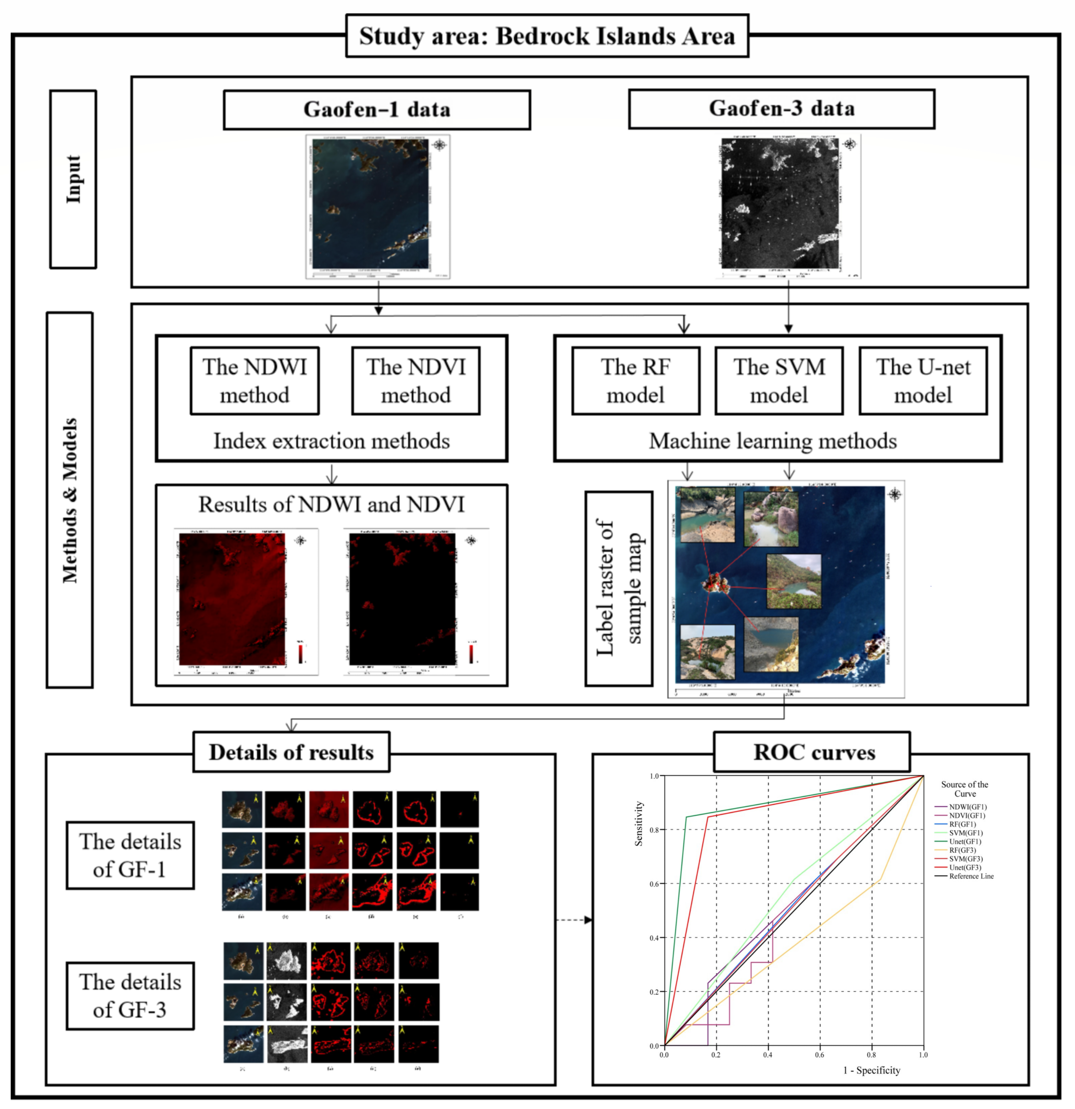
To address the specific challenges of freshwater extraction on bedrock islands, this study proposes and evaluates a U-Net-based deep learning framework. Focusing on islands outside the Pearl River Estuary, China, we integrate Gaofen-1 (GF-1) optical and Gaofen-3 (GF-3) synthetic aperture radar (SAR) imagery to leverage complementary information. The primary objectives are: (1) to develop a high-precision freshwater extraction model tailored to island environments; (2) to rigorously compare the performance of the proposed U-Net model against representative traditional methods (NDWI, NDVI) and classical ML algorithms (RF, SVM); and (3) to validate the model’s effectiveness in mitigating typical interference factors like seawater intrusion and cloud cover. The overall research workflow is illustrated in Figure 1. We hypothesize that the U-Net model will demonstrate superior accuracy and robustness, providing a reliable tool for island freshwater resource management.

From a global policy perspective, the United Nations Sustainable Development Goal 6 (SDG 6) calls for universal access to clean water and the protection of water-related ecosystems. Remote sensing has been identified as a key technology for tracking SDG indicator 6.3.2 (proportion of bodies of water with good ambient water quality), especially in data-scarce regions such as small islands where traditional in situ monitoring networks are sparse or nonexistent [5]. The integration of optical and SAR satellite data offers unique advantages for operational SDG monitoring by enabling all-weather observation capabilities that can track both the spatial extent and, potentially, the quality of surface freshwater resources.

2. Materials and Methods

2.1. Study Area

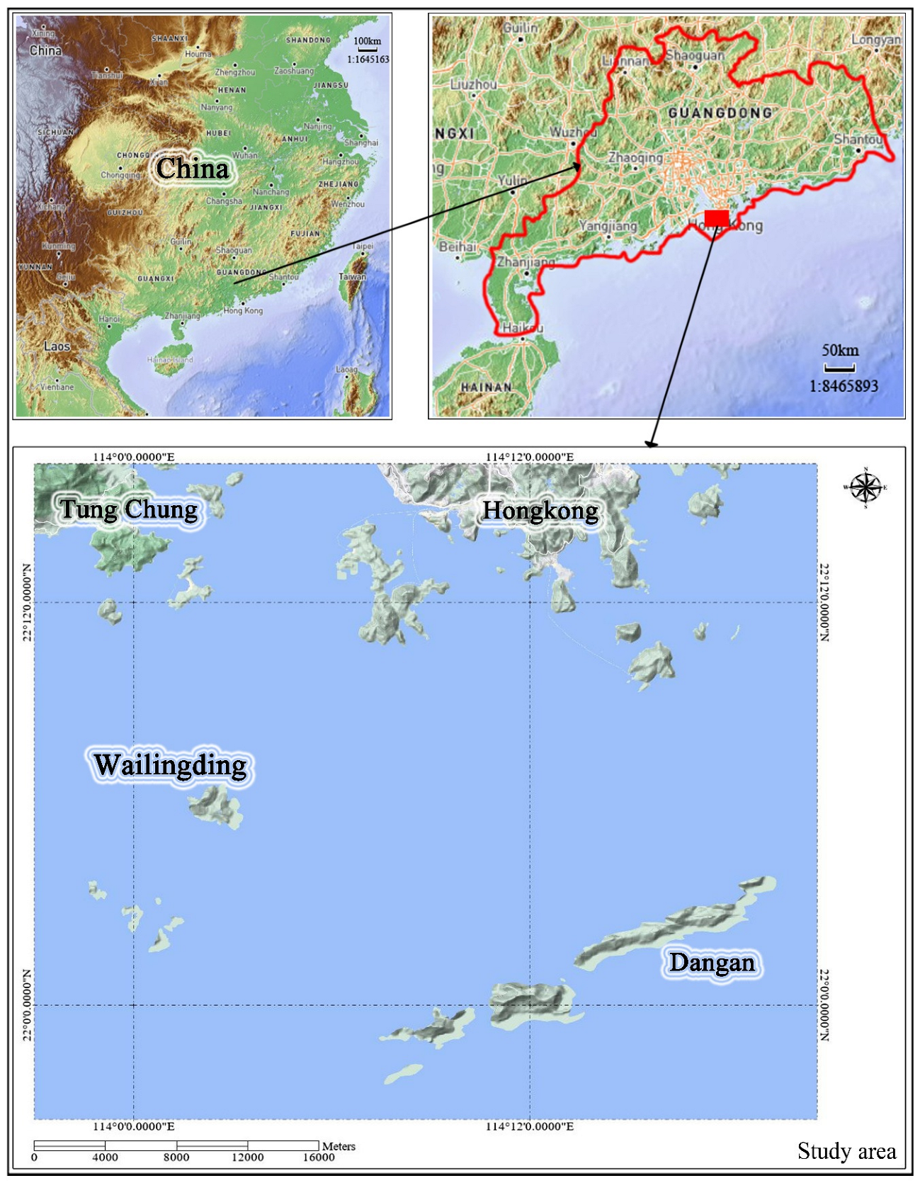
The study area encompasses approximately 2053.5 km² of the Pearl River Estuary in southern China, spanning longitudes 113°57′49″ E to 114°21′40″ E and latitudes 21°58′20″ N to 22°12′40″ N (Figure 2). This region faces a significant environmental challenge: freshwater scarcity. Field investigations revealed that island communities primarily depend on expensive shipped water or limited small-scale reservoirs, while desalination remains cost-prohibitive.

The freshwater systems on these islands are intimately linked to local ecosystems. Surface freshwater bodies, including small ponds, reservoirs, and shallow wetlands, serve as critical habitats for aquatic organisms and provide drinking water sources for terrestrial fauna. These surface water features are the primary target of this study. The groundwater-dependent ecosystems—including riparian vegetation and small wetland patches sustained by shallow groundwater discharge—are particularly sensitive to changes in freshwater availability and quality. The chloride ion (Cl⁻) concentration, used in this study as a primary indicator to distinguish freshwater from seawater, also serves as an ecologically relevant parameter, as elevated salinity can exceed the tolerance thresholds of freshwater-dependent species and alter the composition of riparian plant communities.

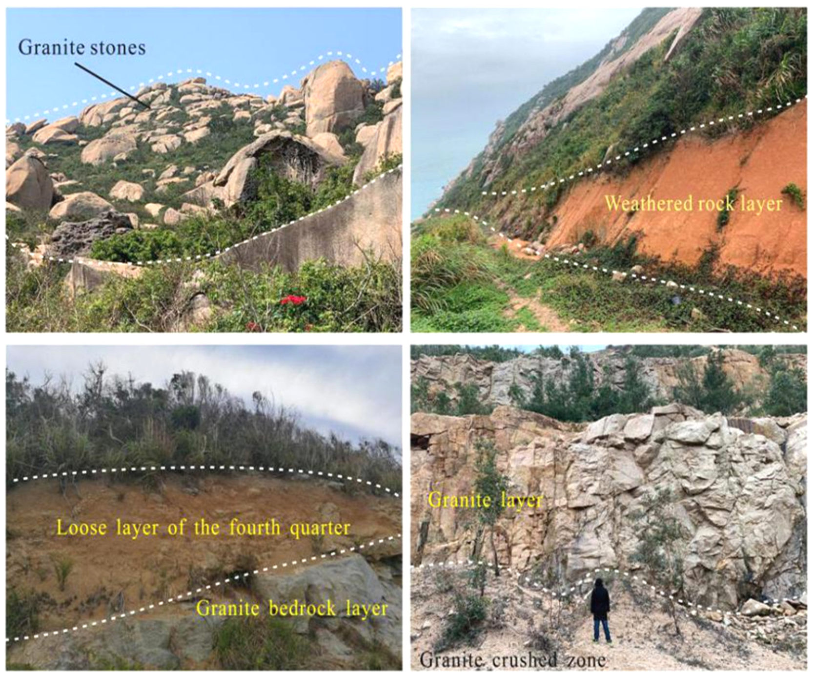
Geologically, the islands are characterized by surface layers of Quaternary weathered rock and loose sediments, underlain by granite bedrock. A notable geomorphological feature is the widespread presence of large, rounded granite boulders. Hydrogeologically, groundwater resources consist of pore water within the Quaternary loose layers and fissure water within the bedrock [26,27] (Figure 3). Critically, the islands’ geology and hydrogeology are highly similar across the study area. Each island constitutes a relatively independent and predominantly natural hydrological system with minimal anthropogenic pollution, making its endogenous freshwater a valuable and potable resource that warrants effective utilization and protection. This geological and hydrological consistency provides a coherent data foundation applicable to regional analysis and modeling approaches.

2.2. The Introduction of GF-1 Data and GF-3 Data

The study utilized data from the GaoFen-1 (GF-1) and GaoFen-3 (GF-3) satellites [28,29]. The GF-1 satellite, launched in 2013, is China’s first high-resolution civil Earth observation satellite. It carries a panchromatic and multispectral (PMS) camera and a multispectral (MSS) camera. The PMS camera provides a panchromatic band (0.45–0.90 μm) at 2-m spatial resolution and four multispectral bands (Blue: 0.45–0.52 μm, Green: 0.52–0.59 μm, Red: 0.63–0.69 μm, Near-Infrared: 0.77–0.89 μm) at 8-m resolution. The MSS camera offers four spectral bands (similar to the PMS multispectral bands) at a coarser 16-m resolution (

Table 1. GF-1 Sensor band parameters.

Sensor	Band	Wavelength (μm)	Spatial Resolution (m)
Panchromatic & Multispectral Camera	1	0.45~0.90	2
	2	0.45~0.52	8
	3	0.52~0.59
	4	0.63~0.69
	5	0.77~0.89
Multispectral Camera	6	0.45~0.52	16
	7	0.52~0.59
	8	0.63~0.69
	9	0.77~0.89

). While GF-1 data provide high spatial resolution, its spectral capabilities (number of bands) are more limited compared to platforms like Landsat 8, which offers additional spectral bands (e.g., coastal aerosol, cirrus, and thermal infrared bands) [28].

The GF-3 satellite, launched in August 2016, is a C-band synthetic aperture radar (SAR) sat ellite [29]. Unlike optical sensors, SAR is active and operates in the microwave spectrum, making it capable of all-weather and day–night imaging, which is particularly advantageous for continuous environmental monitoring. GF-3 features 12 imaging modes with spatial resolutions ranging from 1 m to 500 m and swath widths from 10 km to 650 km, supporting various polarization modes (single, dual, and quad-polarization) (

Table 2. Technical specifications of GF-3 satellite payload.

The Names of the Imaging Modes		Spatial Resolution/m	Breadth/km	Polarization Mode
The slider bunching		1	10	single polarization
Strip imaging mode	Ultra-fine Strip	3	30	single polarization
	FSI	5	50	dual polarization
	FSII	10	100	dual polarization
	SS	25	130	dual polarization
	QPSI	8	30	complete polarization
	QPSII	25	40	complete polarization
Scan SAR imaging mode	NSC	50	300	dual polarization
	WSC	100	500	dual polarization
	GLO	500	650	dual polarization
Wave imaging mode		10	5	complete polarization
Extended incident Angle	The low Angle of incidence	25	130	dual polarization
	High Angle of incidence	25	80	dual polarization

). This flexibility allows GF-3 to support applications in marine surveillance, disaster assessment, water resources management, and meteorology.

2.3. Deep Learning with Convolutional Neural Networks (CNN)

Deep learning, especially Convolutional Neural Networks (CNNs), excels in spatial tasks such as image classification and segmentation [30,31]. This study adopts a CNN-based approach, specifically the U-net architecture, which has proven effective in biomedical segmentation [32] and environmental image analysis. A typical CNN consists of convolutional, pooling, and fully connected layers.

2.3.1. Convolutional Layer

Convolutional layers contain filters whose weights W and bias b are optimized via backpropagation. The computation of a basic neuron is:

$$\mathrm{network}:\{\begin{array}{c}Y=W^{T}X+b\\ Z=f\left(Y\right)\end{array}$$

(1)

where X is the input, W the weight matrix, b the bias, *f*(·) a nonlinear activation, and Z the output. Through local connectivity and weight sharing, convolutional layers efficiently extract local features while reducing parameters. The layer’s operation generalizes this as:

$$X^{\left(l\right)}=f(W^{\left(l\right)}\ast X^{l-1}+b^{\left(l\right)}),l=\mathrm{1,2},3\dots \dots$$

(2)

where ∗ denotes the convolution operation.

2.3.2. Pooling Layer

Pooling (sub-sampling) layers reduce spatial dimensions, lowering computation and providing translational invariance. Typical operations are max pooling and average pooling. Max pooling is expressed as:

$$\begin{array}{l}poo{l}_{\max }(R_k)=\underset{i\in R_k}{\max }(a_i),i=1,2,3\dots \dots \\ poo{l}_{avg}(R_k)={\displaystyle \frac{1}{\left|R_k\right|}}{\displaystyle \sum _{i\in R_k}{a}_i},i=1,2,3\dots \dots \end{array}$$

(3)

where $R_k$ is a local region (e.g., a 2 × 2 window) in the input feature map, and a_i represents the activation values within that region.

2.3.3. Fully Connected Layer

Fully connected layers, placed near the output, connect every neuron to all activations of the previous layer, combining high-level features for final decisions (e.g., classification).

2.3.4. Overview of the U-Net Model

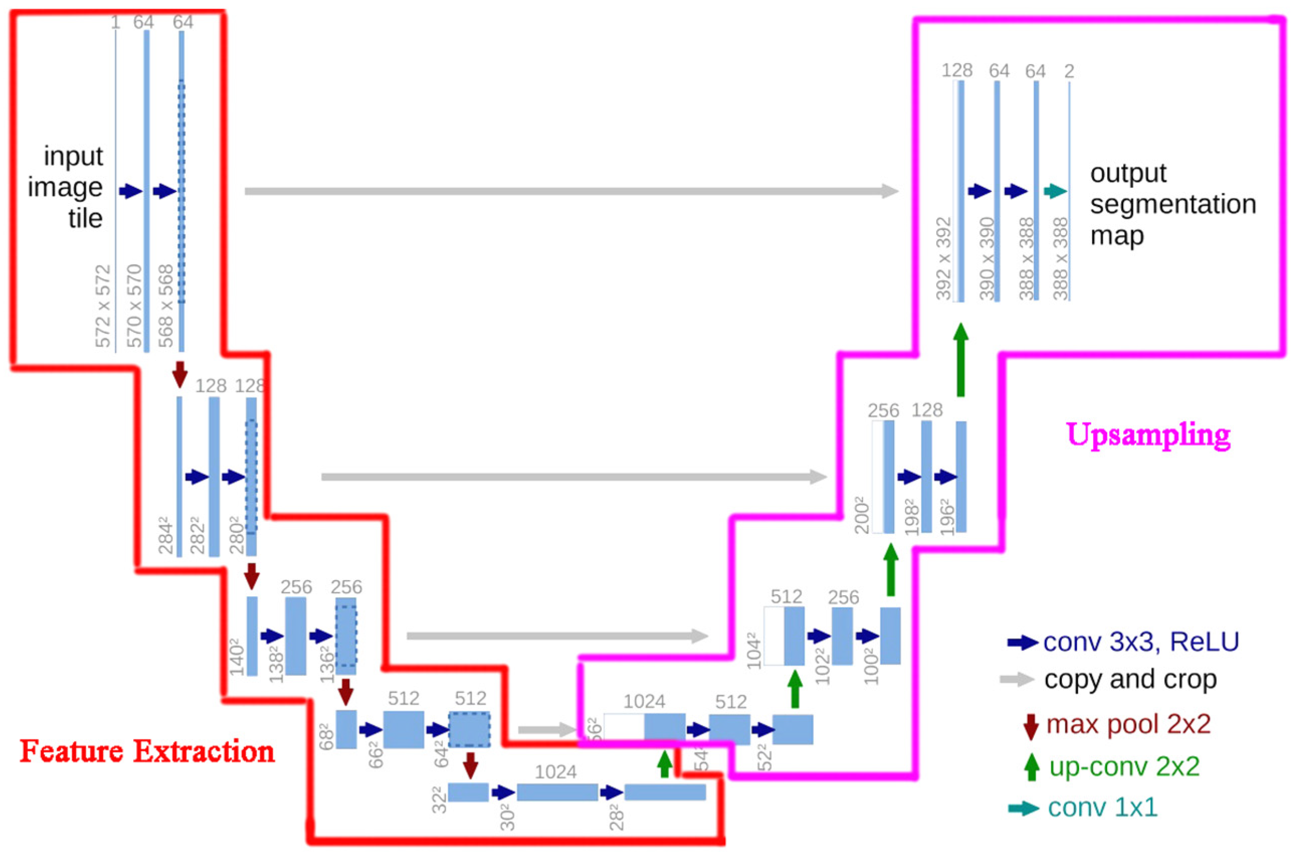
U-net [32,33] is an encoder–decoder architecture with a contracting path that captures context and an expansive path that restores localization (Figure 4). Skip connections concatenate encoder feature maps with decoder layers, preserving fine spatial detail for accurate boundary delineation. Data augmentation (affine transforms, elastic deformations) improves robustness with limited training data, and dropout adds further regularization [34].

2.4. Random Forest (RF)

The Random Forest (RF) algorithm is an ensemble learning method based on multiple decision trees, as proposed by Breiman [35]. In this study, the RF model was constructed by generating multiple bootstrap samples (i.e., random subsets with replacement) from the original training dataset. Each bootstrap sample was used to train an individual decision tree. A key step in optimizing RF performance is the selection of hyperparameters, including the number of trees (n_estimators). Following a parameter tuning process and informed by the findings of Wang et al. (2020) for comparable environmental data, the n_estimators was set to 200 for our analysis [36].

2.5. Support Vector Machine (SVM)

The support vector machine (SVM) is a supervised learning algorithm based on the principle of structural risk minimization, which aims to enhance model generalization by finding a balance between empirical risk and model complexity [37]. Its core objective in binary classification is to identify the optimal hyperplane that maximizes the margin between two classes. For linearly inseparable data, SVM employs kernel functions to nonlinearly map input data into a higher-dimensional feature space, where linear separation becomes feasible [38]. This capability makes SVM particularly suitable for environmental studies where data may be complex and non-linear, yet sample sizes are sometimes limited.

2.6. Normalized Difference Water Index (NDWI) Method

Mcfeeters et al. (1996) proposed the Normalized Difference Water Index (NDWI) using the near-infrared (NIR) and green bands [7]. This index enhances water features by leveraging the typically high reflectance of water in the green band and its strong absorption in the NIR band. Consequently, NDWI can effectively suppress certain non-water features, such as built-up areas and mountain shadows, thereby making water bodies more distinct in the resulting imagery [39]. The NDWI is calculated as follows (Equation (4)), where for GF-1 satellite images, B2 and B4 represent the reflectance of the green and NIR bands, respectively:

$$\mathrm{NDWI}={\displaystyle \frac{\mathrm{B}2-\mathrm{B}4}{B2+\mathrm{B}4}}$$

(4)

The optimal threshold for freshwater extraction using NDWI was determined to be 0.15 through iterative experimentation using the Otsu method, which maximizes inter-class variance between water and non-water pixels [40]. For NDVI, the threshold was set to −0.25, where pixels with NDVI values below this threshold were classified as potential water bodies based on the characteristic low reflectance of water in both red and NIR bands.

2.7. Normalized Difference Vegetation Index (NDVI) Method [41]

The NDVI, primarily designed for vegetation monitoring, can also be utilized for water body delineation based on spectral characteristics. Water bodies generally exhibit low reflectance in both the red and NIR bands, appearing dark in NDVI imagery and creating a distinct grayscale contrast with brighter features like vegetation. Therefore, a suitable threshold applied to an NDVI image can be used to extract water bodies. The NDVI is calculated according to the following formula (Equation (5)), where R1 and R2 denote the reflectance of the red and NIR bands, respectively:

$$\mathrm{NDVI}={\displaystyle \frac{\mathrm{R}2-\mathrm{R}1}{\mathrm{R}2+\mathrm{R}1}}$$

(5)

2.8. Physical Basis for Freshwater Identification

The identification of surface freshwater from satellite imagery relies on distinct physical properties that differentiate freshwater from seawater and other land cover types.

2.8.1. Optical Remote Sensing Principles

Freshwater exhibits characteristic spectral signatures due to its unique optical properties. In the visible spectrum, particularly the green band (0.52–0.59 um), freshwater typically shows relatively higher reflectance compared to seawater, because seawater contains suspended sediments, dissolved organic matter, and phytoplankton that increase absorption and scattering [7,39]. In the near-infrared (NIR) band (0.77–0.89 um), both freshwater and seawater exhibit strong absorption, but freshwater bodies generally show slightly higher absorption due to their lower turbidity and absence of suspended particles. This spectral contrast between the green and NIR bands forms the physical basis for water indices such as NDWI [7]. Additionally, the spectral signature of freshwater in coastal island environments can be influenced by surrounding vegetation, bedrock shadows, and shallow water depth, which may cause spectral confusion with non-water features.

2.8.2. SAR Remote Sensing Principles

Synthetic Aperture Radar (SAR) provides complementary information for freshwater identification through microwave backscatter characteristics. The key physical parameters include: (1) Dielectric constant: The dielectric constant of freshwater (~80) differs significantly from that of seawater (~70–75) due to salinity differences, affecting the microwave reflectivity of water surfaces [42]. (2) Surface roughness: Calm freshwater surfaces act as specular reflectors, producing very low backscatter values (dark appearance in SAR images), while seawater surfaces are typically rougher due to wind-induced waves, resulting in higher backscatter [43]. (3) Polarization response: Different polarization modes (HH, HV, VV) capture distinct scattering mechanisms. For freshwater extraction, the HH polarization is particularly sensitive to surface scattering from smooth water bodies. The C-band SAR onboard GF-3 (5.3 GHz frequency) provides optimal penetration through cloud cover and vegetation canopy, enabling freshwater detection under adverse weather conditions where optical sensors are limited.

3. Results and Discussion

3.1. The Preprocessing of GF-1 Data and GF-3 Data

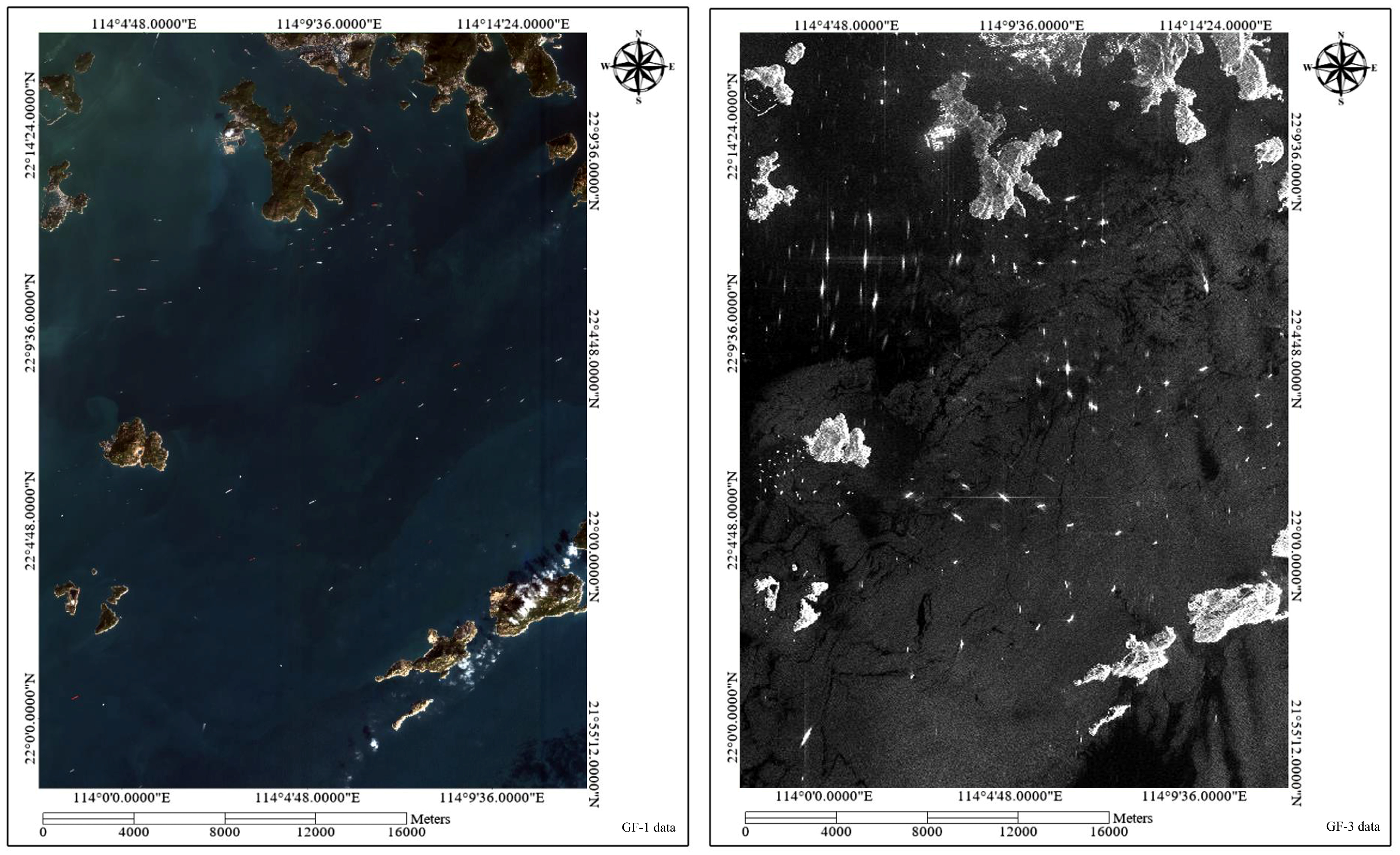
The study used GF-1 data (GF1_PMS2_E114.2_N22.1_20170121 _L1A0002136162-MSS2; available at http://www.rscloudmart.com/ (accessed on 5 June 2022)). Then, ENVI software (ENVI 5.5) [44] was used to pre-process the GF-1 data using the radiometric calibration and atmospheric correction modules; the result of preprocessing is shown in Figure 5. For GF-3 SAR data, the following preprocessing steps were applied: (1) Speckle filtering: A Lee filter with a 7 × 7 window size was applied to reduce the inherent speckle noise of SAR imagery while preserving edge details [43]. (2) Radiometric calibration: The digital number (DN) values were converted to backscatter coefficients (sigma0) using the calibration factors provided in the GF-3 metadata. (3) Terrain correction: Range-Doppler terrain correction was performed using a digital elevation model (DEM) to correct geometric distortions caused by topographic variations. (4) Polarization processing: The HH polarization channel was used for freshwater extraction, as it provides optimal sensitivity to smooth water surfaces. The original GF-3 data (Figure 5) used “GF3_SAY_FSI_002767_E113.9_N22.0_20170217_ L1A_HHHV_L10002192808” file obtained from https://www.cresda.com (accessed on 5 June 2022). The GF-3 map belongs to an FSI imaging mode and has 5 m spatial resolution (Figure 5).

3.2. Applications and Results in U-Net of CNN (Deep Learning), RF, SVM, NDWI & NDVI

3.2.1. Building Label Data of Machine Learning Models

The construction of labeled data is a prerequisite for training supervised machine learning models. The process involved the following steps: (1) Field survey: Hydrogeological field surveys were conducted on Wailingding Island and surrounding islands in early 2017 (dry season). Water samples were collected from 23 wells and 15 springs located adjacent to identified surface freshwater bodies (ponds and reservoirs) across the study area. These sampling points were selected because they are hydraulically connected to surface freshwater bodies and their water quality can represent the freshwater characteristics of the adjacent surface water features. (2) Water quality analysis: Chloride ion (Cl⁻) concentration was measured for each sample using ion chromatography. Based on international drinking water standards (WHO guidelines and Chinese national standard GB 5749-2022(GB 5749-2022; Standards for Drinking Water Quality. National Health Commission of the People’s Republic of China: Beijing, China, 2022.)), a threshold of 250 mg/L was used to distinguish freshwater (Cl⁻ < 250 mg/L) from saline/brackish water (Cl⁻ ≥ 250 mg/L). (3) Label mask generation: Point-based Cl⁻ measurements were converted to pixel-wise label masks using buffer zones in ENVI software. For each freshwater sampling point, a circular buffer zone with radius proportional to the estimated freshwater extent was created. These buffer zones were then rasterized to generate binary masks (freshwater = 1, non-freshwater = 0). (4) Dataset statistics: The final labeled dataset contained approximately 15,000 freshwater pixels (~0.12 km²) and 185,000 non-freshwater pixels (~1.48 km²) for GF-1 imagery, and similar proportions for GF-3 imagery. (5) Training/validation split: The dataset was divided into 70% for training (14 islands) and 30% for validation (6 islands), ensuring spatial independence between training and validation samples.

3.2.2. The Workflow Based on U-Net

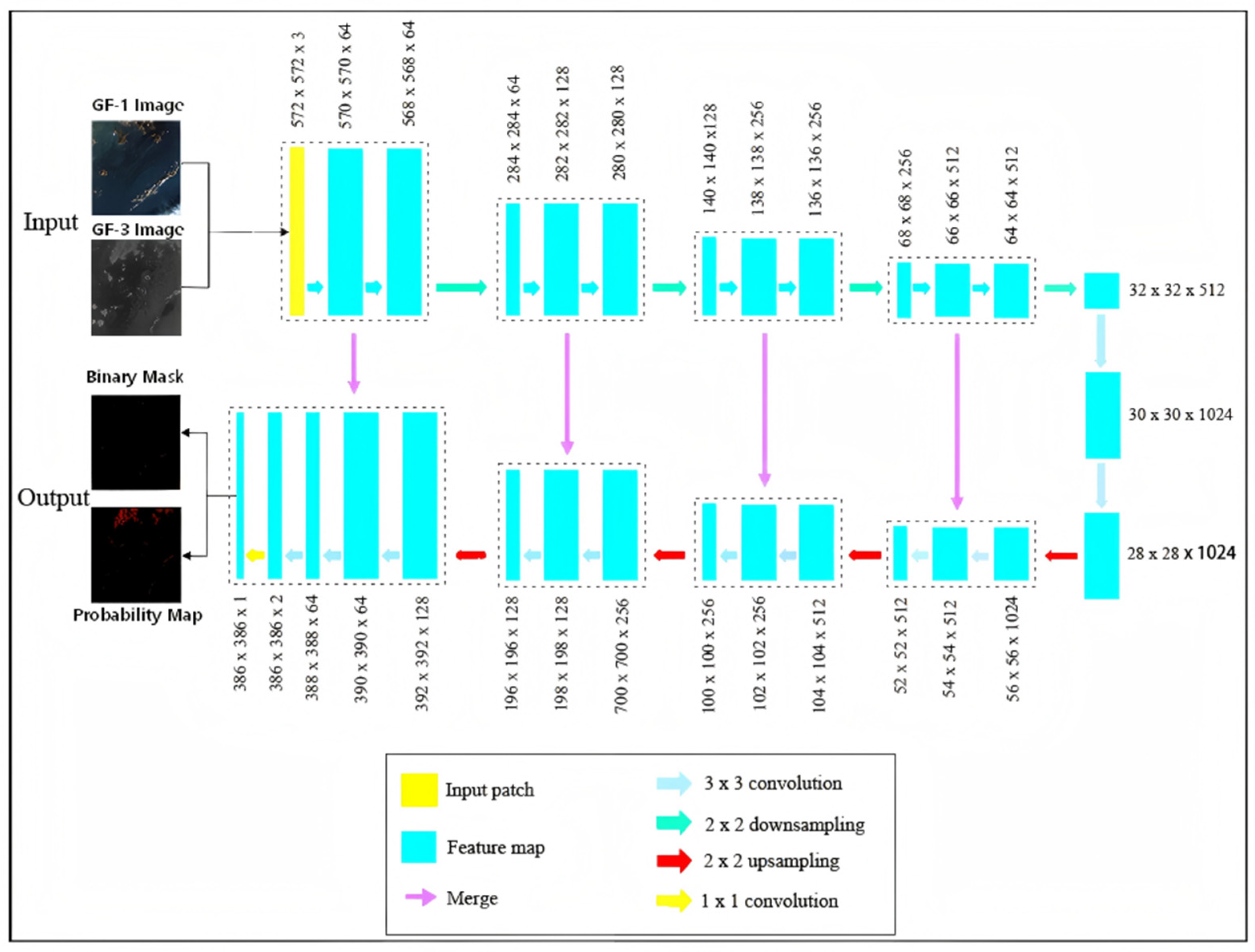
The overall workflow for water body extraction using the U-Net model in this study is illustrated in Figure 6. The process began with the assignment of input parameters and the preparation of training sample data. Model development was implemented on the TensorFlow 2.12 [32]. Following training and testing phases, a trained convolutional neural network (CNN) model was obtained, which was then applied to generate the final extraction results.

The model architecture, depicted in Figure 6 for a single image patch, was based on the U-Net framework [34]. It comprised five levels (representing different pixel resolutions) with a total of 27 convolutional layers. The input patch size was set to 572 × 572 pixels, utilizing three spectral bands. The output was a class activation raster, which was subsequently converted into a binary water mask for comparison against the labeled ground truth data.

A key parameter of this architecture is its contextual field of view, which defines the extent of the surrounding area influencing the classification of each central pixel during training. For this U-Net implementation, the contextual field of view was 140 × 140 pixels. Employing an input patch size (572 × 572) larger than this field allowed for more efficient batch training and faster classification. To enable the model to learn features larger than 140 × 140 pixels, a down-sampling strategy was applied to the training rasters. The U-Net model was implemented with the following hyperparameters: the number of filters started from 64 in the first convolutional layer, doubling at each downsampling step (64, 128, 256, 512, 1024); the kernel size was 3 × 3 for all convolutional layers, with padding to maintain spatial dimensions; the activation function was ReLU for all layers except the final output layer, which used sigmoid activation for binary classification; the loss function was Binary Cross-Entropy (BCE) loss; the optimizer was Adam with an initial learning rate of 1 × 10⁻⁴; the batch size was set to 16 patches per batch; the number of training epochs was 100 with early stopping based on validation loss (patience = 10). Data augmentation techniques, including random horizontal and vertical flips, random rotation (+/−15 degrees), and elastic deformations, were applied during training to improve model robustness [34]. The model was trained using a 70/30 split of the labeled data for training and validation, respectively. To account for potential spatial autocorrelation between nearby pixels, the training and validation samples were selected from different islands to ensure spatial independence. The training process took approximately 4 h on an NVIDIA GeForce RTX 2080 Ti GPU (NVIDIA Corporation, Santa Clara, CA, USA).

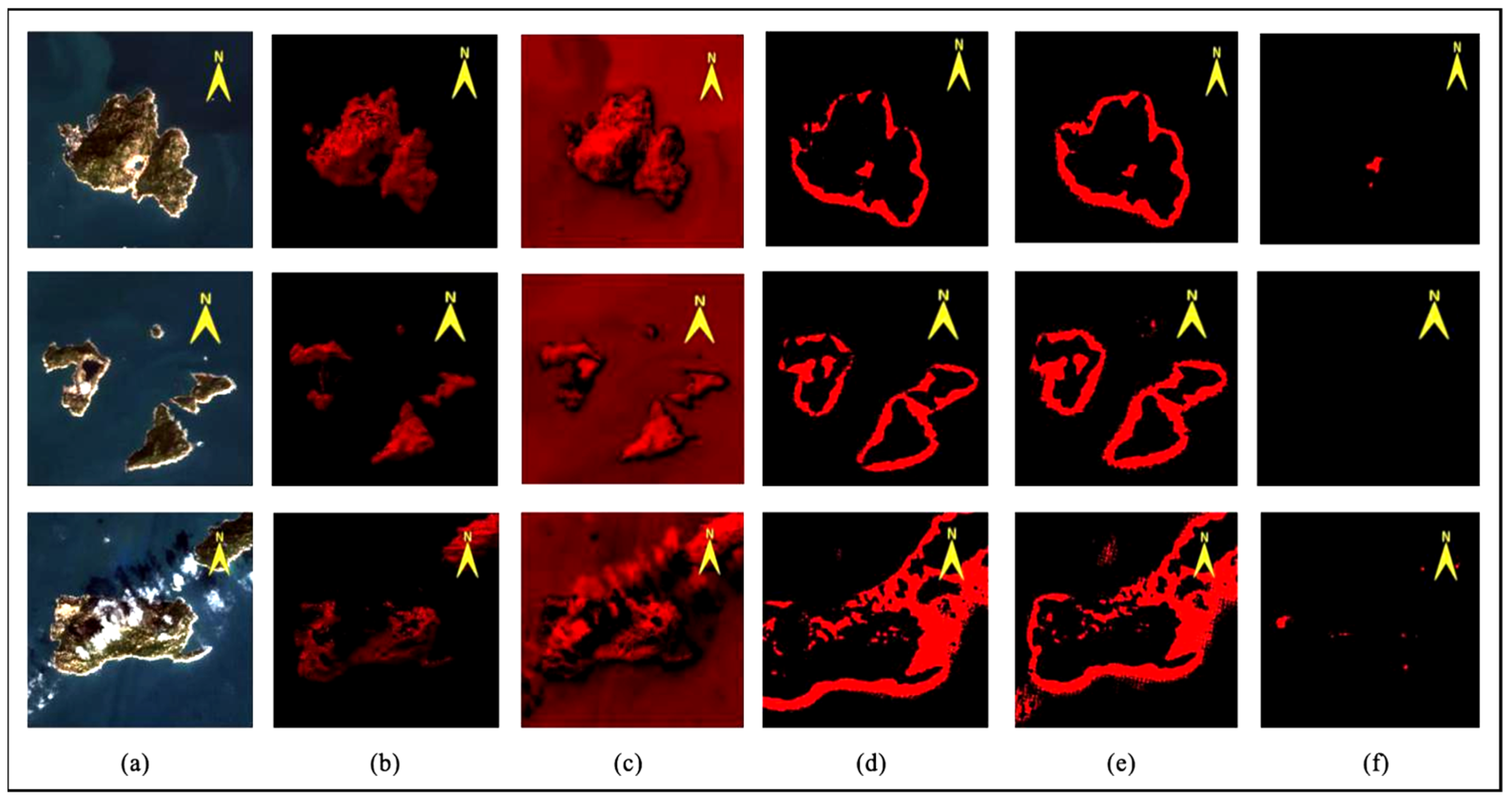
For Cewang Island (second map in Figure 7a), NDWI and NDVI indicated potential surface water, and RF and SVM extracted this area. U-Net, however, did not extract it. This is likely because this water body had a high Cl⁻ concentration and spectral characteristics similar to seawater. The U-Net model, trained on input samples from GF-1 data, may have classified it as non-freshwater. For Dangang Island (third map in Figure 7a), cloud cover impeded accurate classification by RF and SVM, but U-Net produced an accurate result, demonstrating robustness to cloud interference.

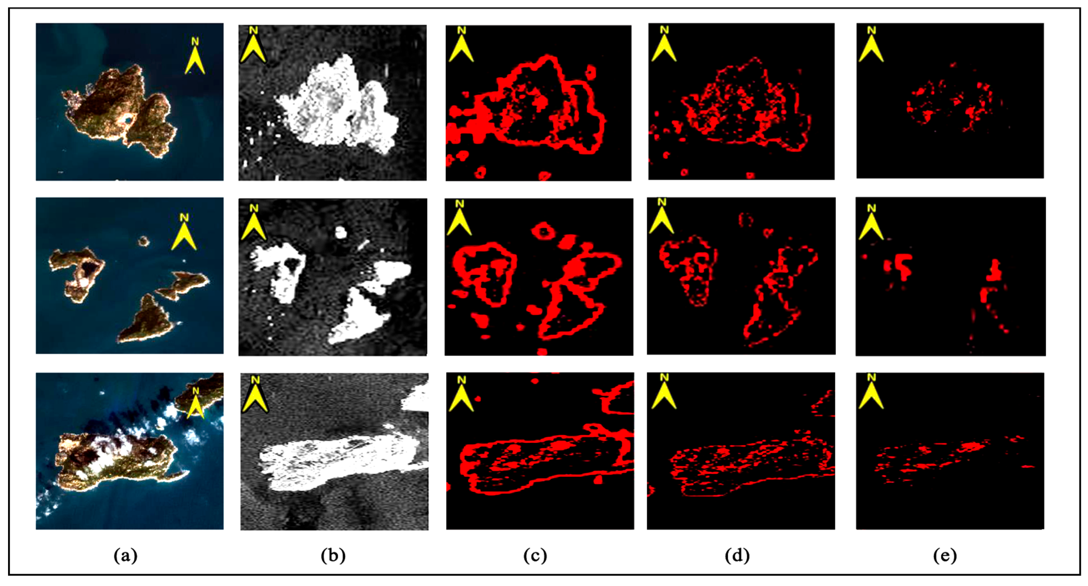
The analysis was extended to GF-3 satellite data (Figure 8). For Wailingding Island, RF and SVM results from GF-3 data still included coastal misclassification, while U-Net effectively discriminated the coastal region. For Cewang Island, all three methods (RF, SVM, and U-Net) applied to GF-3 data extracted the saline water area, a shortcoming not observed in the U-Net results from GF-1 data. For Dangang Island, GF-3 data was unaffected by clouds present in the GF-1 image, leading to better extraction results across all methods for GF-3 in this case.

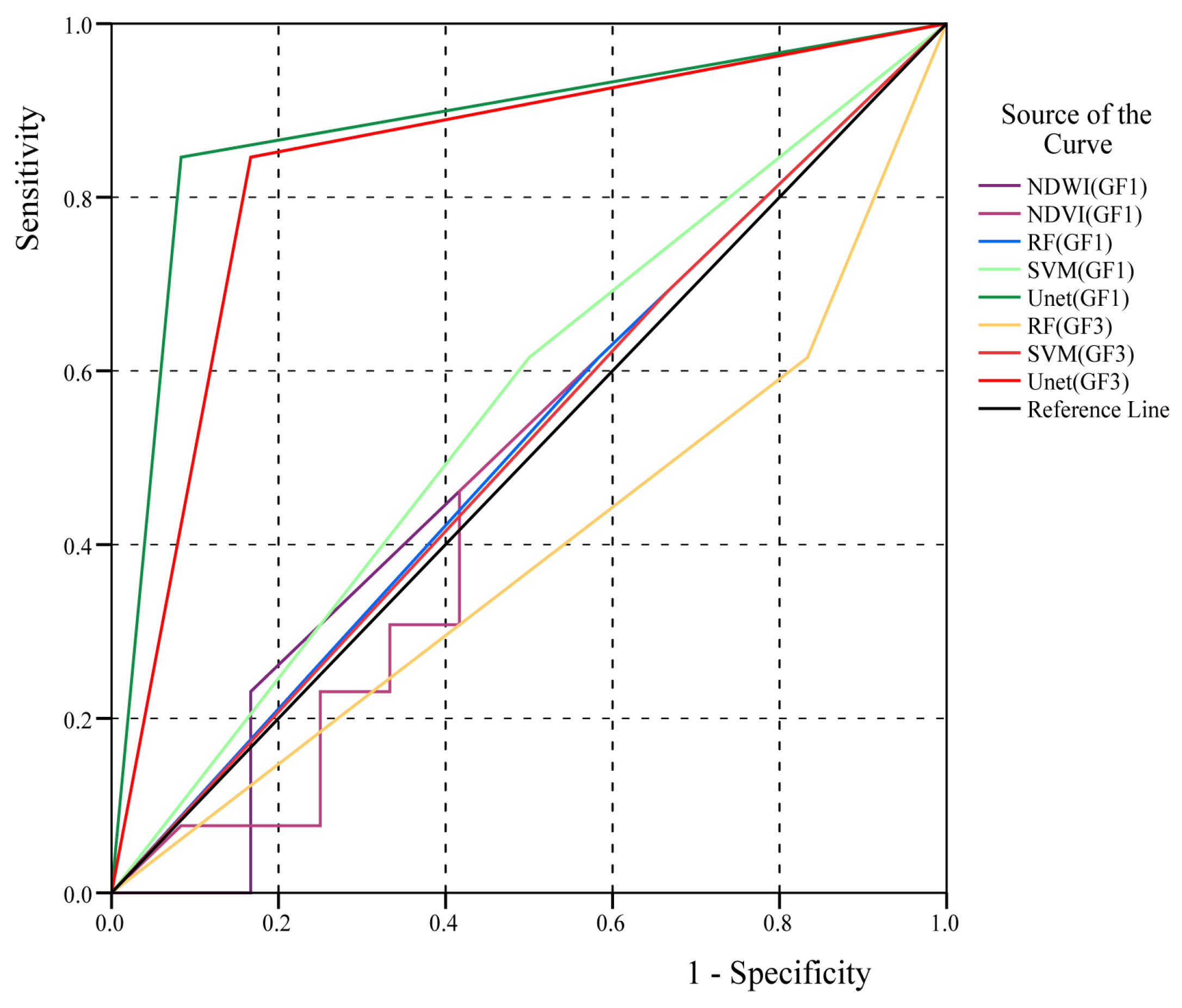
To quantitatively compare the methods, Receiver Operating Characteristic (ROC) curves were analyzed [45,46] (Figure 9,

Table 3. The ROC curves analysis data sheet.

Test Variables	Area (AUC)	Standard Error	Sig.b	95% Confidence Interval
				Lower Limit	Upper Limit
NDWI_GF1	0.513	0.119	0.913	0.280	0.746
NDVI_GF1	0.487	0.119	0.913	0.254	0.721
RF_GF1	0.516	0.118	0.892	0.285	0.747
SVM_GF1	0.558	0.117	0.624	0.328	0.787
U-net_GF1	0.881	0.076	0.001	0.733	1.000
RF_GF3	0.391	0.115	0.355	0.166	0.616
SVM_GF3	0.513	0.118	0.913	0.282	0.744
U-net_GF3	0.840	0.087	0.004	0.670	1.000

). For GF-1 data, the U-Net model achieved the highest Area Under the Curve (AUC) value (AUC_U-net_GF-1 = 0.881), followed by SVM (AUC_SVM_GF-1 = 0.558), RF (AUC_RF_GF-1 = 0.516), NDWI (AUC_NDWI_GF-1 = 0.513), and NDVI (AUC_NDVI_GF-1 = 0.487). The lower AUC values for RF and SVM suggest misclassifications, while the index-based methods (NDWI, NDVI) showed limited discriminative power. For GF-3 data, U-Net also yielded the best performance (AUC_U-net_GF-3 = 0.840).

The relatively low AUC values observed for traditional methods (NDWI, NDVI, RF, SVM) around 0.5 can be attributed to the unique challenges of freshwater extraction in coastal island environments: (1) Spectral similarity: In coastal settings, freshwater bodies often exhibit spectral characteristics similar to seawater due to mixing at the freshwater–seawater interface, making spectral index-based methods less effective. (2) Complex terrain: The bedrock islands feature rugged terrain with extensive shadows and mixed pixels at water–land boundaries, which traditional methods cannot adequately distinguish. (3) Limited training samples: The RF and SVM models were trained on a relatively small dataset that may not fully capture the variability of freshwater appearances in different conditions. (4) Binary classification challenge: Unlike typical water body extraction tasks that distinguish water from land, this study specifically aims to separate freshwater from seawater, a more nuanced task that requires finer spectral discrimination. The U-Net model’s superior performance demonstrates its ability to learn complex spatial-spectral features that traditional methods cannot capture, particularly the contextual information around freshwater bodies that helps distinguish them from seawater and shadows. It is important to note that the optical (GF-1) and SAR (GF-3) data capture fundamentally different physical properties of water surfaces. Optical sensors detect spectral reflectance characteristics, while SAR sensors detect microwave backscatter from surface roughness and dielectric properties. Consequently, the spatial patterns of segmentation results from these two data sources may differ significantly, as each method responds to different aspects of the freshwater–seawater interface. The ROC curves, however, measure each model’s classification performance on its respective dataset independently, rather than spatial overlap between the two segmentation maps. The consistency in AUC values indicates that both models achieve comparable classification accuracy, even though their spatial outputs differ due to the distinct physical information captured by each sensor type. The ROC curves were constructed using independent test points manually selected from verified freshwater bodies (positive samples) and non-freshwater regions (negative samples) across the study area. The number of test points is limited by the natural scarcity of freshwater bodies on bedrock islands, but each point was carefully verified to ensure ground-truth accuracy. The ROC analysis evaluates each model’s classification performance on its respective sensor dataset independently, which explains why the AUC values are consistent despite spatial differences in the segmentation outputs. Statistical significance testing using the DeLong test [47] confirmed that U-Net’s AUC was significantly higher than all other methods (p < 0.01 for both GF-1 and GF-3 data).

In summary, the U-Net model demonstrated superior precision and accuracy for surface freshwater extraction from both GF-1 and GF-3 data in this study. These findings suggest that U-Net can be a valuable tool for efficiently mapping surface freshwater resources on islands, supporting related planning and management efforts.

3.2.3. Application and Results Based on GF-1 and GF-3

It should be noted that Figure 7 and Figure 8 display the probability maps output by the U-Net model, where the red color saturation represents the predicted probability of each pixel being classified as freshwater. To present the final binary segmentation results, a threshold of 0.5 was applied to the probability maps to generate binary masks (freshwater = 1, non-freshwater = 0). The binary classification results are consistent with the probability maps shown, with higher-probability regions corresponding to the identified freshwater areas. Figure 7a presents the original remote sensing images for three islands. For Wailingding Island (first map in Figure 7a), surface water is visible in the south–central area, which was identified as freshwater based on chloride ion (Cl⁻) test reports. The Normalized Difference Water Index (NDWI) and Normalized Difference Vegetation Index (NDVI) results (Figure 7b and Figure 7c, respectively) provided spectral indices related to surface water presence but could not specifically delineate the freshwater area. In contrast, all three machine learning methods—Random Forest (RF), Support Vector Machine (SVM), and U-Net—successfully extracted the south-central freshwater area (Figure 7d–f). However, RF and SVM also misclassified parts of the coastal area as freshwater, whereas U-Net more effectively distinguished between freshwater and coastal zones.

3.3. Environmental Implications and Influencing Factors

The surface freshwater distribution extracted by the proposed U-Net framework is influenced by a complex interplay of environmental factors that merit further discussion. The geological homogeneity of granite bedrock across the study area, while advantageous for model generalization, also implies that the freshwater system is heavily reliant on seasonal precipitation patterns and is vulnerable to hydroclimatic variability. The freshwater lens dynamics on these islands are intrinsically linked to the balance between recharge from rainfall and losses through evapotranspiration and subsurface outflow to the ocean [4,48].

From an ecosystem perspective, the freshwater bodies mapped in this study serve as critical habitats and water sources for island biota. The spatial distribution of freshwater directly influences the extent and health of riparian vegetation, which in turn stabilizes shorelines and provides organic matter inputs to nearshore marine ecosystems. Monitoring changes in freshwater extent over multi-temporal scales could therefore serve as a valuable proxy for assessing island ecosystem resilience under ongoing environmental change.

The successful discrimination between freshwater and seawater using the U-Net model, as validated by Cl⁻ measurements, has important implications for water quality management under the SDG 6 framework. Zhang et al. (2023) demonstrated that remote sensing-derived water clarity metrics can serve as effective proxies for evaluating SDG indicator 6.3.2 on Hainan Island [5]. The methodological framework developed in this study could be adapted for similar SDG monitoring applications on bedrock islands, where the integration of water extent mapping with water quality parameters (e.g., salinity, turbidity) would provide a more comprehensive assessment of freshwater resource status. Future research could explore the use of multi-temporal GF-1/GF-3 imagery to establish a baseline and track changes in freshwater availability in response to seasonal precipitation variability, drought events, and long-term climate trends, thereby supporting evidence-based water governance in island environments.

3.4. Limitations and Future Research Directions

Despite the promising results, several limitations should be acknowledged. First, the model was trained and validated using data from a single season (dry season, early 2017), which may not capture the full range of hydrological conditions, particularly the wet season when surface water extent expands considerably. Future studies should incorporate multi-temporal imagery to assess the model’s performance across different seasons and under extreme hydrological events.

Second, the reliance on Cl⁻ concentration as the primary indicator for freshwater identification, while geochemically robust, provides only a binary classification (freshwater vs. seawater). Future work could explore the potential for retrieving continuous salinity gradients from combined optical-SAR data, which would provide more nuanced information for ecological risk assessment in transitional coastal zones.

Third, the transferability of the trained U-Net model to other island types (e.g., coral atolls, volcanic islands, sandy barrier islands) remains to be tested. The distinct hydrogeological characteristics of different island types—such as the highly permeable substrates of atolls versus the impermeable bedrock of the current study area—may require model retraining or architectural modifications to maintain performance.

Fourth, atmospheric and illumination effects should be considered. For optical data (GF-1), varying atmospheric conditions (haze, aerosols) and illumination angles may affect the spectral signatures of freshwater, potentially reducing model accuracy. For SAR data (GF-3), changes in wind speed and surface roughness can alter backscatter characteristics, potentially causing misclassification of calm freshwater as rough seawater.

Fifth, the geographic transferability of the trained model is limited. The model was developed specifically for granite bedrock islands in the Pearl River Estuary. Transferability to other island types (coral atolls, volcanic islands, sandy barrier islands) or other geographic regions requires further validation with locally collected training data.

4. Conclusions

This study aimed to enhance the extraction efficiency and discriminative capability for mapping surface freshwater on bedrock islands. The study area was located outside the Pearl River Estuary, China. The relatively homogeneous geological and geomorphological features of this region provided a suitable context for testing machine learning approaches. We utilized high-resolution optical satellite imagery (GF-1) and synthetic aperture radar data (GF-3) as primary data sources. A reference dataset of freshwater sources, derived from field surveys and water quality tests (primarily Cl⁻ concentration), served as sample data for model training and validation.

Our results demonstrated that the U-net deep learning model outperformed other benchmark methods in extracting surface freshwater from bedrock islands using GF-1 data, achieving the highest AUC value on the ROC curve. Furthermore, the U-net model effectively distinguished surface freshwater regions from coastal zones and saltwater-intruded areas in GF-1 imagery, and maintained performance under cloud cover when using GF-3 radar data. In contrast, other machine learning methods and traditional index-based approaches yielded less accurate results with notable misclassifications.

Field surveys, including geological assessments and Cl⁻ ion tests, corroborated the model-derived extents. The U-net-based method presents advantages in terms of automation efficiency and reduced reliance on extensive manual interpretation for freshwater extraction on bedrock islands. This suggests its potential for application to other island types (e.g., sandy, volcanic), although careful adaptation of the sample set is necessary. This study also highlights the complementary value of integrating optical (GF-1) and radar (GF-3) imagery to mitigate the limitations of optical data under adverse weather conditions.

The U-Net-based freshwater extraction framework developed in this study offers a practical and scalable solution for environmental monitoring agencies tasked with tracking freshwater availability on bedrock islands. When combined with periodic water quality sampling, this approach can contribute to the assessment of SDG indicator 6.3.2 and support adaptive water resource management strategies in the face of climate variability.

Future research should extend this framework to multi-temporal monitoring, enabling the detection of seasonal and interannual changes in freshwater extent that may signal emerging environmental stresses—such as drought-induced freshwater contraction or storm-surge-induced salinization—before they escalate into critical water shortages for island communities and ecosystems.

References

1. White, I.; Falkland, T. Management of freshwater lenses on small Pacific islands. Hydrogeol. J. 2010, 18, 227–246. [Google Scholar] [CrossRef]
2. Lu, J.J.; Li, S.H. Improvement of TM data water body identification technology. Environ. Remote Sens. 1992, 7, 17–24. [Google Scholar] [CrossRef]
3. Vorosmarty, C.J.; Green, P.; Salisbury, J.; Lammers, R.B. Global water resources: Vulnerability from climate change and population growth. Science 2000, 289, 284–288. [Google Scholar] [CrossRef] [PubMed]
4. Panthi, J.; Boving, T.B.; Pradhanang, S.M. The contraction of freshwater lenses in barrier island: A combined geophysical and numerical analysis. J. Hydrol. 2024, 635, 131371. [Google Scholar] [CrossRef]
5. Qiu, R.; Wang, S.; Shi, J.; Shen, W.; Zhang, W.; Zhang, F.; Li, J. Sentinel-2 MSI Observations of Water Clarity in Inland Waters across Hainan Island and Implications for SDG 6.3.2 Evaluation. Remote Sens. 2023, 15, 1600. [Google Scholar] [CrossRef]
6. Yang, C.J.; Xu, M. Discussion on water extraction method of remote sensing information mechanism. Geogr. Res. 1998, 17, 86–89. [Google Scholar]
7. McFeeters, S.K. The use of the Normalized Difference Water Index (NDWI) in the delineation of open water features. Int. J. Remote Sens. 1996, 17, 1425–1432. [Google Scholar] [CrossRef]
8. Wang, Z.H.; Yi, S.Z. Comparative study of different index model methods in water remote sensing extraction. Sci. Technol. Eng. 2007, 4, 534–537. [Google Scholar]
9. Xia, S.; Ruan, R.Z.; Yan, M.C. Study on water information extraction method based on TM image. J. Nanjing For. Univ. Nat. Sci. Ed. 2012, 36, 29–35. [Google Scholar] [CrossRef]
10. Cao, R.L.; Li, C.J.; Liu, L.Y. Area extraction and change monitoring of Miyun Reservoir based on water index. Sci. Surv. Mapp. 2008, 33, 158–160. [Google Scholar]
11. Feyisa, G.L.; Meilby, H.; Fensholt, R.; Proud, S.R. Automated Water Extraction Index: A new technique for surface water mapping using Landsat imagery. Remote Sens. Environ. 2014, 140, 23–35. [Google Scholar] [CrossRef]
12. Ding, F. Experimental research on water information extraction based on new water index (NWI). Sci. Surv. Mapp. 2009, 34, 155–157. [Google Scholar] [CrossRef]
13. Li, Y.; Gong, X.; Guo, Z.; Xu, K.; Hu, D.; Zhou, H. An index and approach for water extraction using Landsat–OLI data. Int. J. Remote Sens. 2016, 37, 3611–3635. [Google Scholar] [CrossRef]
14. Lacaux, J.P.; Tourre, Y.M.; Vignolles, C.; Ndione, J.A.; Lafaye, M. Classification of ponds from high-spatial resolution remote sensing: Application to Rift Valley Fever epidemics in Senegal. Remote Sens. Environ. 2007, 106, 66–74. [Google Scholar] [CrossRef]
15. Chen, J.B.; Liu, S.X.; Wang, C.Y. Research on urban water body extraction based on knowledge decision tree. Remote Sens. Inf. 2013, 28, 29–33. [Google Scholar] [CrossRef]
16. Li, J.J. Study on Accurate Extraction of Frozen Lake Water Based on SVM Proximity Assimilation Filter Model. Master’s Thesis, Xi’an University of Science and Technology, Xi’an, China, 2009. [Google Scholar]
17. Zhu, C.M.; Luo, J.C.; Shen, Z.F.; Li, J.L. Adaptive iterative extraction of small linear river water assisted by DEM. Acta Geod. Cartogr. Sin. 2013, 42, 277–283. [Google Scholar]
18. Yang, W.L.; Yang, M.H.; Qi, H.X. Extraction of TM image water using BP neural network. Sci. Surv. Mapp. 2012, 37, 148–150. [Google Scholar] [CrossRef]
19. Li, C.C.; Zhang, G.S.; Shen, L. Water information extraction of remote sensing image based on AdaBoost algorithm. Sci. Surv. Mapp. 2013, 38, 104–106. [Google Scholar] [CrossRef]
20. Li, A.M.; Liu, Y.; Zhang, X.; Wang, L.; Wu, L.C.; Xia, G.P. Effects of different index methods on surface water extraction. Water Conserv. Inf. 2019, 5, 34–39. [Google Scholar] [CrossRef]
21. Liao, H.Y.; Wen, T.H. Extracting urban water bodies from high-resolution radar images: Measuring the urban surface morphology to control for radar’s double-bounce effect. Int. J. Appl. Earth Obs. Geoinf. 2020, 85, 102003. [Google Scholar] [CrossRef]
22. Hu, S.S.; Qin, J.X.; Ren, J.C.; Zhao, H.M.; Ren, J.; Hong, H.R. Automatic extraction of water inundation areas using Sentinel-1 data for large plain areas. Remote Sens. 2020, 12, 243. [Google Scholar] [CrossRef]
23. Maxwell, A.E.; Warner, T.A.; Fang, F. Implementation of machine-learning classification in remote sensing: An applied review. Int. J. Remote Sens. 2018, 39, 2784–2817. [Google Scholar] [CrossRef]
24. Aliihsan, S. A survey on global thresholding methods for mapping open water body using Sentinel-2 satellite imagery and normalized difference water index. Arch. Comput. Methods Eng. 2021, 28, 1335–1347. [Google Scholar] [CrossRef]
25. Zhu, X.X.; Tuia, D.; Mou, L.C.; Xia, G.S.; Zhang, L.P.; Xu, F.; Fraundorfer, F. Deep learning in remote sensing: A comprehensive review and list of resources. IEEE Geosci. Remote Sens. Mag. 2017, 5, 8–36. [Google Scholar] [CrossRef]
26. Huang, Y.K.; Xia, F.; Chen, G.N. Some geological and geomorphological characters of islands off the Pearl River Estuary. Mar. Sci. Bull. 1985, 4, 46–51. [Google Scholar]
27. Xu, H.L.; Wang, D.Q.; Deng, Z.D.; Ding, Z.B.; Liu, Z.X.; Wang, G.Y.; Ni, B.R. Application of remote sensing fuzzy assessment method in groundwater potential in Wailingding Island. J. Supercomput. 2020, 76, 3646–3658. [Google Scholar] [CrossRef]
28. Lu, C.L.; Bai, Z.G. Characteristics and typical applications of GF-1 satellite. In Proceedings of the 2015 IEEE International Geoscience and Remote Sensing Symposium (IGARSS), Milan, Italy, 26–31 July 2015; IEEE: New York, NY, USA, 2015; pp. 1246–1249. [Google Scholar] [CrossRef]
29. Zhang, Q. System design and key technologies of the GF-3 satellite. Acta Geod. Cartogr. Sin. 2017, 46, 269–277. [Google Scholar] [CrossRef]
30. LeCun, Y.; Bengio, Y.; Hinton, G. Deep learning. Nature 2015, 521, 436–444. [Google Scholar] [CrossRef] [PubMed]
31. Krizhevsky, A.; Sutskever, I.; Hinton, G.E. ImageNet classification with deep convolutional neural networks. Commun. ACM 2017, 60, 84–90. [Google Scholar] [CrossRef]
32. Wongsuphasawat, K.; Smilkov, D.; Wexler, J.; Wilson, J.; Mané, D.; Fritz, D.; Krishnan, D.; Viégas, F.B.; Wattenberg, M. Visualizing dataflow graphs of deep learning models in TensorFlow. IEEE Trans. Vis. Comput. Graph. 2018, 24, 1–12. [Google Scholar] [CrossRef] [PubMed]
33. Hinton, G.E.; Salakhutdinov, R.R. Reducing the dimensionality of data with neural networks. Science 2006, 313, 504–507. [Google Scholar] [CrossRef] [PubMed]
34. Ronneberger, O.; Fischer, P.; Brox, T. U-Net: Convolutional neural networks for biomedical image segmentation. In Medical Image Computing and Computer-Assisted Intervention—MICCAI 2015; Navab, N., Hornegger, J., Wells, W.M., Frangi, A.F., Eds.; Springer: Cham, Switzerland, 2015; Volume 9351, pp. 234–241. [Google Scholar] [CrossRef]
35. Breiman, L. Random forests. Mach. Learn. 2001, 45, 5–32. [Google Scholar] [CrossRef]
36. Wang, N.; Cheng, J.H.; Zhang, H.Y. Application of U-net model to water extraction with high resolution remote sensing data. Remote Sens. Land Resour. 2020, 32, 35–42. [Google Scholar]
37. Wang, Z.W.; Sun, J.J.; Yu, Z.Y. Overview of research on remote sensing image classification based on support vector machines. Comput. Sci. 2016, 43, 11–17. [Google Scholar]
38. Chen, Q.; Tian, J.; Huang, H.N. SVM segmentation of SAS images based on statistics and texture features. J. Instrum. 2013, 34, 1413–1420. [Google Scholar]
39. Xu, H.Q. Modification of normalised difference water index (NDWI) to enhance open water features in remotely sensed imagery. Int. J. Remote Sens. 2006, 27, 3025–3033. [Google Scholar] [CrossRef]
40. Otsu, N. A threshold selection method from gray-level histograms. IEEE Trans. Syst. Man Cybern. 1979, 9, 62–66. [Google Scholar] [CrossRef]
41. Ding, L.D.; Yu, W.H.; Tan, Z.H. Production of remote sensing image of water flood in Poyang lake area based on MODIS. Remote Sens. Land Resour. 2007, 19, 82–85. [Google Scholar]
42. Ulaby, F.T.; Long, D.G. Microwave Radar and Radiometric Remote Sensing; Artech House: Norwood, MA, USA, 2014. [Google Scholar]
43. Lee, J.S.; Pottier, E. Polarimetric Radar Imaging: From Basics to Applications; CRC Press: Boca Raton, FL, USA, 2009. [Google Scholar]
44. Xue, L. Application of IDL and ENVI redevelopment in hyperspectral image preprocessing. In Computer and Computing Technologies in Agriculture IV; Li, D., Liu, Y., Chen, Y., Eds.; Springer: Berlin/Heidelberg, Germany, 2011; Volume 347, pp. 403–409. [Google Scholar] [CrossRef]
45. Rahul, N.; Das, J.; Raman, B. A hybrid of deep learning and hand-crafted features based approach for snow cover mapping. Int. J. Remote Sens. 2019, 40, 759–773. [Google Scholar] [CrossRef]
46. Mingote, V.; Miguel, A.; Ortega, A.; Lleida, E. Optimization of the area under the ROC curve using neural network supervectors for text-dependent speaker verification. Comput. Speech Lang. 2020, 63, 101079. [Google Scholar] [CrossRef]
47. DeLong, E.R.; DeLong, D.M.; Clarke-Pearson, D.L. Comparing the areas under two or more correlated receiver operating characteristic curves: A nonparametric approach. Biometrics 1988, 44, 837–845. [Google Scholar] [CrossRef] [PubMed]
48. Thissen, L.; Greskowiak, J.; Gaslikova, L.; Massmann, G. Climate change impact on barrier island freshwater lenses and their transition zones: A multi-parameter study. Hydrogeol. J. 2024, 32, 1417–1431. [Google Scholar] [CrossRef]
Figure 1. Study flow for extraction of surface freshwater in bedrock islands.
Environments 13 00358 g001
Figure 2. Location interactive map of the study area.
Environments 13 00358 g002
Figure 3. The geological and geomorphologic images of islands.
Environments 13 00358 g003
Figure 4. The flow of U-net [34].
Environments 13 00358 g004
Figure 5. The map of GF-1 data and GF-3 data after preprocessing.
Environments 13 00358 g005
Figure 6. The flow of U-net in this study.
Environments 13 00358 g006
Figure 7. Classification results for surface freshwater mapping using GF-1 satellite imagery obtained from (a) original map of GF-1; (b) NDWI of GF-1; (c) NDVI of GF-1; (d) RF of GF-1; (e) SVM of GF-1; (f) U-net of GF-1.
Environments 13 00358 g007
Figure 8. Classification results for surface fresh water mapping using GF-3 satellite imagery ob-tained from, (a) Original map of GF-1, (b) Original map of GF-3, (c) RF of GF-3, (d) SVM of GF-3, (e) U-net of GF-3.
Environments 13 00358 g008
Figure 9. Comparison of the performance of different models for surface freshwater mapping using the ROC graph.
Environments 13 00358 g009