PM2.5 Organosulfates/Organonitrates and Organic Acids at Two Different Sites on Cyprus: Time and Spatial Variation and Source Apportionment

Abstract

Long-term particulate matter (PM) chemical composition measurements were performed in Cyprus at two different sites (an urban/traffic site (“LIMTRA”) and a remote/background site (“AGM”)) in an effort to assess (i) the spatial and temporal variability of fine (PM2.5) particulate matter in the eastern Mediterranean; (ii) the main sources contributing to their levels and their relationship with the characteristics of the sampling location; and (iii) the enhancement effect of local anthropogenic and natural biogenic sources on PM levels. To this end, the simultaneous determination of 118 individual Secondary Organic Aerosol (SOA) components (carboxylic acids, organosulfates, and organonitrates) was performed. The “AGM” station showed average SOA yields more than three times higher than those at the “LIMTRA” station (15 ng∙m⁻³ and 4.4 ng∙m⁻³, respectively), whilst the organonitrate levels were higher at “LIMTRA” than at “AGM” (3.3 ng∙m⁻³ and 1.8 ng∙m⁻³, respectively). The most abundant SOA species were hydroxy-acetone sulfate, glycolic acid sulfate, and lactic acid sulfate (21 ng∙m⁻³ at “LIMTRA” and 84 ng∙m⁻³ at “AGM”). The highest SOA load was observed in spring at “AGM” (18 ng∙m⁻³) and in summer at “LIMTRA” (6.8 ng∙m⁻³). Two statistical factorization tools, Principal Component Analysis and Positive Matrix Factorization, were applied to extract common patterns and point to possible SOA sources and SOA formation pathways; the different categorization approaches produced similar results.

1. Introduction

Secondary organic aerosols (SOAs) constitute a significant portion of atmospheric particulate matter. The formation and composition of SOAs are driven by the presence of biogenic and anthropogenic volatile organic compounds (VOCs) and oxidants in the atmosphere, and their interactions with the condensed phase components [1]. The complexity of SOAs arises from their dynamic physicochemical properties, which vary depending on precursor type, reaction pathway, and environmental factors such as ambient temperature (AT), relative humidity (RH), and aerosol acidity [2,3]. In recent studies, it has been revealed that SOAs show different trends during the year, depending on their origin. On the one hand, SOAs of biogenic origin (BSOAs) are intensively formed during the warm season. They undergo oxidation processes, transforming them into less volatile compounds that condense in the aerosol liquid phase [1]. Higher temperatures and intense UV light from solar radiation facilitate these processes [4]. As a result, it is expected to find higher levels of BSOAs during summer and autumn. At the same time, the formation pathways of SOAs from anthropogenic sources (ASOAs) have received attention as emission contributions to PM pollution from human activities. Nevertheless, the variety and complexity of SOAs make it difficult to track the formation pathways of different ASOAs during the pollution process, especially in complicated urban environments. A better understanding of SOA occurrence and properties is crucial, as they influence climate and affect human health, with many species having been characterized as potentially Reactive Oxygen Species (ROS) [5,6,7] and shown to cause respiratory toxicity [8]. In the Mediterranean basin, SOA formation exhibits pronounced spatiotemporal variability. Notably, coastal urban areas like Cyprus experience enhanced SOA yields due to the convergence of high levels of marine emissions, shipping pollutants, and photochemically aged anthropogenic VOCs [9]. Field studies in this region have highlighted the competitive and/or synergistic effects of atmospheric oxidants (O₃/NO_x) in driving SOA production, the dual role of aerosol acidity derived from the presence of SO₂ and SO₄²⁻, and the relatively high RH conditions that favor particle-phase oligomerization [10].

Despite the recent advances, there are still gaps in our knowledge of the characteristics of oxygenated SOA tracers and their sources, especially organosulfates (OSs) and organonitrates (ONs), in environments with anthropogenic and biogenic sources [11]. A limited number of field studies have attempted to simultaneously measure OSs/ONs and other SOA compounds, such as organic acids (OAs), or correlate their abundances [12]. Additionally, from an analytical point of view, few studies have addressed the development of analytical methods for SOA compound determination, and of those only few have attempted to quantify both polar/non-polar and low/high-molecular-weight components using the same analytical method and authentic standards [13].

This study aims to provide new information concerning these knowledge gaps using High-Resolution Mass Spectroscopy to characterize various SOA markers at background (“AGM”) and urban (“LIMTRA”) sites in Cyprus, taking advantage of the availability of PM2.5 samples that are collected throughout the year. It also aims to identify the major influencing factors of OS and ON formation by simultaneously determining the levels of OAs with different chemical structures (dicarboxylic, monocarboxylic, hydroxy-, aromatics, and terpenoids) and OSs/ONs from nine different groups (aliphatic, isoprenoid, monoterpenoid, sesquiterpenoid, aromatic, trimethyl-benzoic, and naphthalenic groups). By integrating source apportionment analysis, we elucidate the roles of SO₂-driven aerosol acidity [14], oxidant competition (O₃ vs. NO₃∙) [15], and anthropogenic–biogenic interactions [16] in shaping SOA composition. Using this approach, the present study investigates the aerosols in the Eastern Mediterranean, an area of great importance as it lies at the crossroad between diverse air masses from anthropogenic and natural sources in Europe, Asia, and N. Africa.

2. Materials and Methods

2.1. Sampling

Samples were collected in 2019 from two sites in Cyprus with different characteristics. The first one is at Agia Marina Xyliatou (AGM) and is a remote/background station and the other one is at Limassol (LIMTRA) and is an urban/traffic station. Both these stations are part of the Air Quality Monitoring Network in Cyprus. More details about the sampling sites can be found elsewhere [17]. At both sampling sites (AGM and LIMTRA), PM2.5 samples were collected on pre-weighted quartz fiber filters with a 47 mm diameter (Pall Tissuquartz 2500 QAT-UP, Pall Laboratory, Port Washington, NY, USA) using low volume samplers (Leckel SEQ 47/50, Sven Leckel, Berlin, Germany) (flow rate: 2.3 m³∙h⁻¹). In total, 84 PM2.5 samples were collected at AGM (January to December of 2019) and 69 PM2.5 samples were collected at LIMTRA (January to October of 2019). Every month, seven samples plus one field blank were collected at each station. The sampling dates were the same for both sites for comparison reasons. After sampling, the filters were stored at <−18 °C until analysis. Before analysis, the filters were cut in half; one half of the AGM samples was analyzed for organic acids and the other one was analyzed for organosulfates and organonitrates. Regarding the LIMTRA filters, only one half was analyzed for OSs and ONs. At both stations, during the sampling, meteorological parameters and conventional pollutants (NO, NO₂, CO, SO₂, and O₃) were monitored. Ions were only determined at the AGM station (CH₃SO₃⁻, Cl⁻, NO₂⁻, Br⁻, NO₃⁻, SO₄²⁻, C₂O₄²⁻, Na⁺, NH₄⁺, K⁺, Mg²⁺, Ca²⁺, and PO₄³⁻).

2.2. Analysis

2.2.1. Method A: Organic Acids

One half of the filters was extracted twice with 5 mL of methanol (LC-MS grade) via sonication for 20 min each time. The extracts (10 mL total volume) were concentrated to approximately 2–3 mL in a rotary evaporator and the remaining extract was filtered through 0.13 μm PTFE filters using a polypropylene/polyethylene syringe. The filtered extract was further condensed under a gentle stream of N₂ until it was dry. The sample was reconstituted with 0.4 mL of a succinid-d4 acid and phthalic-d4 acid methanol solution (100 ng∙mL⁻¹), used as internal standards. Sample analysis was performed using an ultra-high performance liquid chromatograph (1290 Infinity II, Agilent Technologies, USA) coupled with a quadrupole time-of-flight mass spectrometer (6550 iFunnel Q-TOF MS, Agilent Technologies, Santa Clara, CA, USA). The mass spectrometer was equipped with an electrospray ionization source (Dual Agilent Jet Stream Ionization). Analytes were separated using an Agilent InfinityLab Poroshell 120 SB-C18 (2.1 × 100 mm, 1.9 μm particle size, Agilent Technologies, USA). The mobile phase consisted of eluent A (UPW, 0.1% acetic acid) and eluent B (9:1 ACN–MeOH, 0.1% acetic acid). The flow rate was set at 0.4 mL min⁻¹ and the gradient elution procedure was as follows: 100% A at 0–0.5 min; 100% A reduced to 85% at 0.5–4.0 min; 85% A reduced to 5% at 4–15 min; 5% A maintained at 15–18 min; 5% A increased to 100% at 18–25 min; 100% A was then maintained for 3 min. The column temperature was set at 30 °C and the injection volume was 5 μL. The mass spectrometer was operated in negative mode with a nebulizer gas pressure of 35 psi. The voltages of the capillary, fragmentor, and octopole RF were set at 3500, 200, and 750 V, respectively. The scanning range for MS and MS/MS was 50–350 m/z, while the scan rate was 1 spectrum/sec. Data acquisition and evaluation were performed using Mass Hunter B.09.00 software.

The analytical method was developed and validated in-house using commercially available reference standards to determine a total of 25 organic acids (OAs). More specifically, 8 dicarboxylic acids (DCAs), 5 monocarboxylic acids (MCAs), 6 aromatic acids (AROMAs), 3 hydroxycarboxylic acids (HCAs), and 3 pinene SOA tracers (PNAs) were determined using this method (

Table A1. Quality control data for method A, including categorization, m/z, reproducibility at two levels, linearity, and traceability.

OA Control Standards
				100 ng/mL		1 μg/mL
Name	Abb.	Group	m/z	R (%) ± SD	RSDR% (n = 6)	R (%) ± SD	RSDR% (n = 6)	R2	LOD (ng/mL, n = 6)	LOQ (ng/mL, n = 6)
propionic acid	C3	MCA	73.0290	-	-	88.3 ± 9.52	9.87	0.9916	164	497
malonic acid	diC3	DCA	103.0032	-	-	54.2 ± 2.48	4.33	0.9996	86	260
succinic acid	diC4	DCA	117.0188	99.8 ± 2.04	2.1	94.1 ± 13.9	12.3	0.9935	2.1	6.3
benzoic acid	BEN	AROMA	121.0290	102 ± 11.1	10.1	121 ± 4.72	4.12	0.9917	14	42
glutaric acid	diC5	DCA	131.0345	75.3 ± 2.54	3.44	86.6 ± 14.2	14.1	0.9935	3.3	10
malic acid	MAL	HCA	133.0137	77.6 ± 3.5	4.47	-	-	0.9962	7.2	22
p-toluic acid	pTOL	AROMA	135.0446	78.8 ± 1.57	2.09	-	-	0.9954	3.1	9.3
adipic acid	diC6	DCA	145.0501	121 ± 0.88	0.75	82.3 ± 7.77	8.77	0.9987	7.2	22
tartaric acid	TAR	HCA	149.0086	-	-	41.5 ± 3.06	6.83	0.9923	85	258
pimelic acid	diC7	DCA	159.0658	126 ± 1.53	1.22	81.9 ± 8.92	10	0.9996	3.4	10
phthalic acid	i-Ph	AROMA	165.0188	80.4 ± 0.57	0.65	73.3 ± 4.53	6.61	0.9971	8.5	26
terephthalic acid	Ph	AROMA	165.0188	124 ± 2.29	1.88	99.6 ± 7.89	8.67	0.9963	2	5.9
isophthalic	t-Ph	AROMA	165.0188	94.2 ± 6.11	6.93	76.2 ± 3.88	5.35	0.9959	1.7	5
suberic acid	diC8	DCA	173.0814	106 ± 17	14.2	-	-	0.9992	3.3	9.9
ketopinic acid	KPA	PNA	181.0865	107 ± 1.08	1.09	-	-	0.997	3	9.1
pinonic acid	PNN	PNA	183.1021	79.7 ± 3.44	4.56	75.9 ± 4.27	6.03	0.997	3.4	10
azelaic acid	diC9	DCA	187.0971	91.8 ± 1.4	1.58	-	-	0.9994	3.1	9.4
citric acid	CIT	HCA	191.0192	-	-	98.7 ± 0.14	0.16	0.9995	289	876
sebacic acid	diC10	DCA	201.1127	94 ± 9.31	9.03	-	-	0.9979	3.3	9.9
benzene-1,2,4-tricarboxylic	TRIM	AROMA	209.0086	100 ± 9.95	8.95	113 ± 8.93	8.62	0.9986	4.4	13
β-caryophyllinic	β-CPA	PNA	253.1440	75.5 ± 4.66	5.87	-	-	0.9971	1.1	3.5
palmitic acid	C16	MCA	255.2324	-	-	103 ± 1.14	1.12	0.9905	85	258
margaric acid	C17	MCA	269.2481	101 ± 3.15	3.29	-	-	0.996	16	48
oleic acid	C18:1	MCA	281.2481	105 ± 2.03	1.98	-	-	0.9976	3.1	9.4
stearic acid	C18	MCA	283.2637	82.8 ± 12.4	7.15	115 ± 12	6.65	0.9969	14	44

). All of them were quantified using authentic standards except for pinic acid, which was determined using commercially available ketopinic acid as a surrogate standard. Spiked filters with all the organic acids as methanol solutions were used to evaluate the optimum pre-treatment conditions (number of extractions, extraction solvent, etc.) and the performance characteristics of the method (see Table A1 of Appendix A). Quality control tests were performed throughout the analysis and field blanks were also analyzed to make any necessary corrections to the quantified results.

2.2.2. Method B: Organosulfates and Organonitrates

Half of the filter was extracted three times with 10 mL, 10 mL, and 5 mL of an acetonitrile/deionized water mixture at a 9:1 ratio via sonication for 30 min per extraction. The extracts (25 mL total volume) were concentrated to approximately 2–3 mL in a rotary evaporator and filtered through 0.13 μm PTFE filters using a polypropylene/polyethylene syringe. The filtered extract was further concentrated under a gentle stream of N₂ until it was dry. The sample was reconstituted with 0.5 mL of an ethyl-d5 sulfate solution in ACN/UPW (9:1), which was used as an internal standard for quantification purposes.

Sample analysis was performed using the UPLC-MS/MS method described for method A. The mobile phase consisted of eluent A (an acetic acid solution, pH 5) and eluent B (ACN). The flow rate was set at 0.3 mL∙min⁻¹ and the gradient elution procedure was as follows: 100% A at 0–2 min; 100% A reduced to 70% at 2–3 min; 70% A reduced to 10% at 3–11 min; 10% A maintained at 11–12% min; 10% A reduced to 5% at 12–12.5 min; 5% A maintained at 12.5–16 min; 5% A increased to 100% at 16–16.5 min; 100% A was then maintained for 2 min. The column temperature was set at 35 °C and the injection volume was 1 μL. The mass spectrometer was operated in negative mode with a nebulizer gas pressure of 40 psi. The voltages of the capillary, fragmentor, and octopole RF were set at 3500, 340, and 750 V, respectively. The scanning range for MS and MS/MS was 100–400 m/z, while the scan rate was 2 spectra/sec.

Detailed information for the development and validation of method B is described in our previous work [17]. Briefly, 12 authentic standards were used to determine a total of 92 organosulfate (OS) and organonitrate (ON) compounds, categorized based on their chemical structure and/or common precursor: 15 isoprene-derived OS (iOSs), 19 monoterpene-derived OS (mtOSs), 10 sesquiterpene-derived OS (stOSs), 10 trimethylbenzene-derived OS (tmbOSs), 4 aromatic OS (aromOSs), 8 naphthalene-derived OS (napOSs), 8 alkyl OS (alkOSs), 14 nitro-oxy organosulfates (NOSs), and hydroxyacetone sulfate, lactic acid sulfate, and glycolic acid sulfate, where were grouped because they all have multiple sources (msOSs). For the compounds determined using a surrogate, any potential isomers with identical or different retention times could not be determined in this study so we presented the sum of all possible isomers. Analytical validation data can be found in

Table A2. Quality control data for method B, including categorization, m/z, reproducibility at two levels, linearity, and traceability.

OS Control Standards
				25 ng/mL		100 ng/mL
Name	Abb.	Group	m/z	R (%) ± SD	RSDR% (n = 10)	R (%) ± SD	RSDR% (n = 10)	R2	LOD (ng/sample, n = 10)	LOQ (ng/sample, n = 10)
methyl sulfate	MeS	alkOS	110.9758	86.1 ± 3.52	3.01	77.5 ± 5.45	3.04	0.9961	11	34
ethyl sulfate	EtS	alkOS	124.9914	89.2 ± 5.67	0.28	85.8 ± 3.41	2.85	0.9988	0.57	1.7
propyl sulfate	PrS	alkOS	139.0071	81.1 ± 4.32	1.15	85.0 ± 1.63	1.19	0.9986	0.80	2.4
hydroxyacetone sulfate	HAS	msOS	152.9863	82.0 ± 5.09	7.43	90.6 ± 3.77	3.09	0.9996	0.12	0.37
glycolic acid sulfate 1	GAS	msOS	154.9656	83.4 ± 4.26	1.76	103 ± 1.22	0.97	0.9969	3.5	11
lactic acid sulfate 1	LAS	msOS	168.9812	78.5 ± 4.72	1.65	92.3 ± 6.36	1.63	0.9988	27	81
phenyl sulfate	PhS	aromOS	172.9914	91.9 ± 5.02	2.63	83.2 ± 4.43	1.34	0.9996	0.77	2.3
benzyl sulfate	BS	aromOS	187.0071	98.1 ± 4.14	1.34	94.5 ± 2.14	1.96	0.9997	0.059	0.18
4-methylphenyl sulfate	p-MPhS	aromOS	187.0071	104 ± 4.40	2.96	108 ± 5.03	3.76	0.9996	2.6	8.0
2- and 3-methylbenzyl sulfate	m+p-MBS	aromOS	201.0227	85.8 ± 3.92	0.42	82.1 ± 2.75	0.79	0.9998	0.078	0.24
octyl sulfate	OctS	alkOS	209.0853	83.2 ± 3.98	1.71	91.3 ± 3.24	1.38	0.9995	0.51	1.5

¹ Recoveries were determined for 250 and 1000 ng/mL.

of Appendix A.

2.3. Statistical Analysis

Mann–Whitney and Kolmogorov tests were used to evaluate the data distribution, with p-values ≤ 0.05 indicating statistically significant differences. Principal Component Analysis (PCA) was applied to study possible differences between sampling sites and for source apportionment purposes. In addition to PCA, Positive Matrix Factorization (PMF) was also used as a factorization statistical tool. EPA PMF 5.0 software and SPSS Software (IBM SPSS statistics, version 24) were used.

3. Results

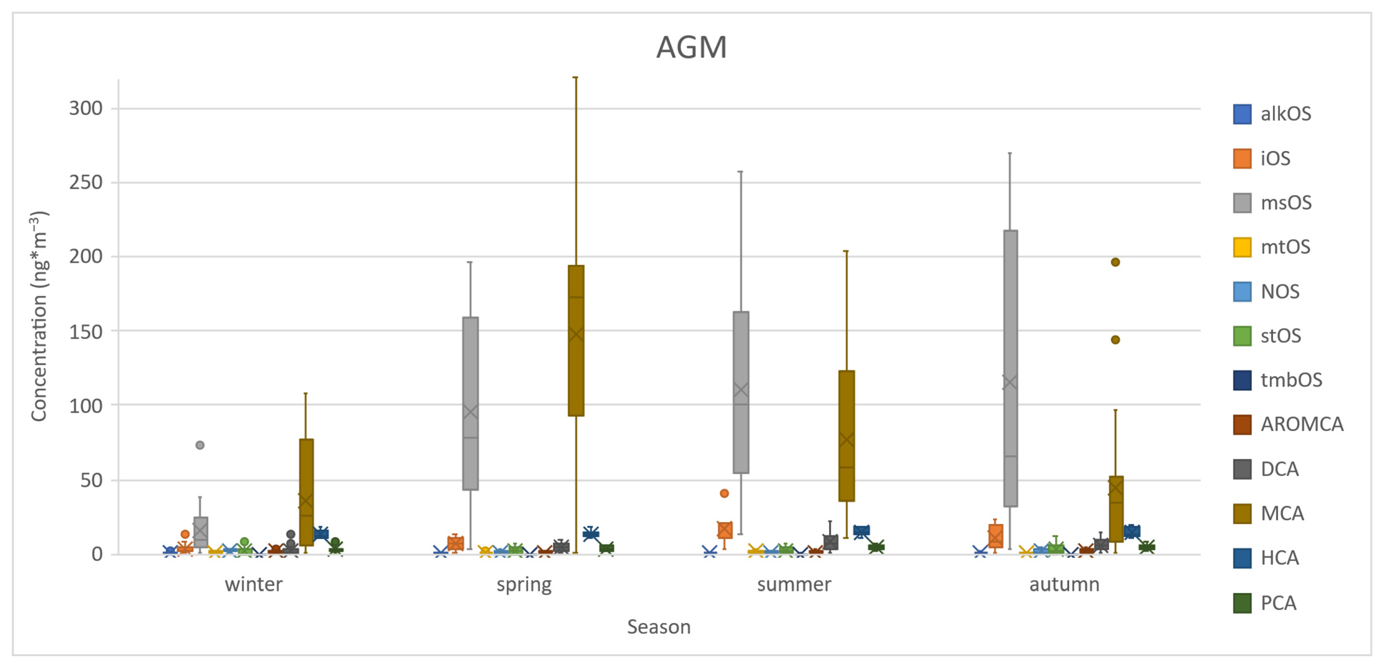
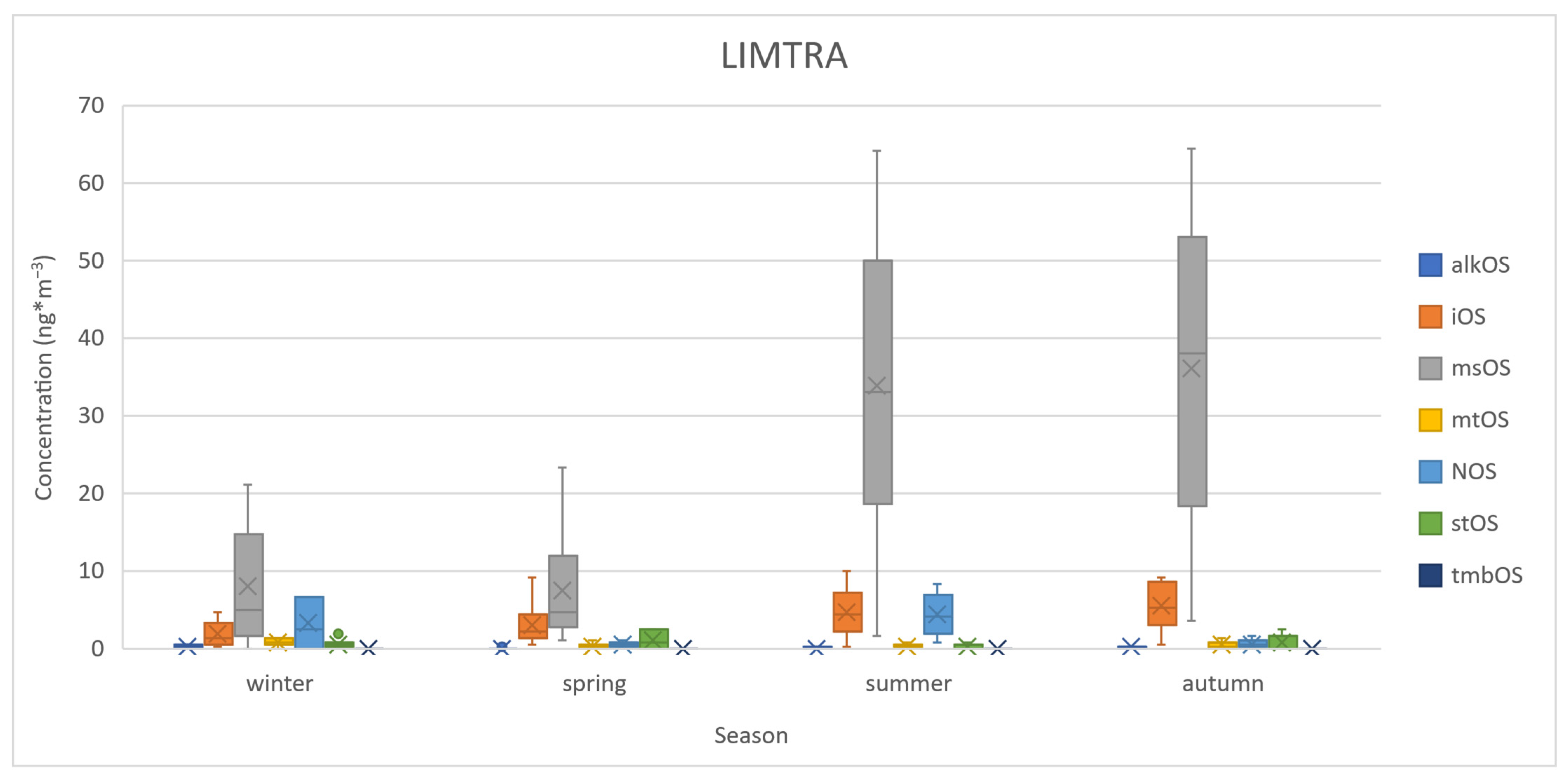
The mean concentration levels (ng∙m⁻³) and standard deviations for each SOA group at the AGM and LIMTRA sites are presented in

Table 1. Seasonal variation in OSs and OAs (ng∙m⁻³) at Agia Marina.

	AGM
	Winter			Spring			Summer			Autumn
	M ± SD	m	Range	M ± SD	M	Range	M ± SD	m	Range	M ± SD	m	Range
alkOSs	0.69 ± 0.51	0.67	2.06	0.63 ± 0.40	0.45	1.30	0.68 ± 0.31	0.66	1.11	0.99 ± 0.35	1.12	1.23
iOSs	3.8 ± 2.9	2.6	12.0	6.8 ± 4.1	6.5	12.7	17.4 ± 8.3	21.3	37.4	10.8 ± 7.7	8.6	21.7
msOSs	16 ± 17	9	73	96 ± 63	78	194	110 ± 68	100	244	115 ± 95	66	266
mtOSs	1.27 ± 0.58	1.18	1.90	0.64 ± 0.50	0.48	1.79	1.77 ± 0.78	1.58	3.04	0.66 ± 0.47	0.59	2.08
NOSs	2.4 ± 0.9	2.4	3.0	1.0 ± 1.2	0.5	3.4	1.3 ± 0.5	1.4	1.6	1.7 ± 1.1	1.3	3.6
stOSs	1.7 ± 2.7	0.1	8.0	2.6 ± 2.6	2.3	6.5	2.3 ± 2.1	1.6	6.3	3 ± 3.3	2.0	12.2
tmbOSs	0.04 ± 0.02	0.04	0.07	0.04 ± 0.05	0.02	0.15	0.11 ± 0.05	0.09	0.18	0.06 ± 0.03	0.05	0.10
AROMCAs	1.6 ± 0.9	1.4	3.6	1.2 ± 0.7	1.2	2.2	1.1 ± 0.7	1.0	2.8	1.8 ± 1	1.7	3.8
DCAs	2.5 ± 2.9	1.3	12.4	4.7 ± 2.7	4.8	8.7	8.9 ± 6.2	7.5	20.8	6.4 ± 3.9	5.4	13.4
MCAs	36 ± 36	26	108	148 ± 84	172	321	76 ± 54	59	193	44 ± 50	35	196
HCAs	12.9 ± 2.8	11.6	7.9	13.5 ± 2.2	12.9	7.8	15.1 ± 2.9	15.1	8.3	14.5 ± 3	13.7	8.7
PNAs	2.8 ± 1.8	2.3	7.6	3.8 ± 1.5	3.3	4.8	4.4 ± 1.4	4.2	5.3	4.6 ± 2.1	4.3	6.7

M: mean; m: median; SD: standard deviation; alkOS: alkyl-OS; iOS: isoprene-derived OS; mtOS: monoterpene-derived OS; NOS: nitro-oxy-OS; stOS: sesquiterpene-derived OS; tmbOS: trimethylbenzene-derived OS; AROMCA: aromatic acid; DCA: dicarboxylic acid; MCA: monocarboxylic acid; HCA: hydroxycarboxylic acid; PNA: pinene SOA tracers.

and

Table 2. Seasonal variation (ng∙m⁻³) in each SOA group during the period of January to October, 2019, in Limassol.

	LIMTRA
	Winter			Spring			Summer			Autumn
	M ± SD	m	Range	M ± SD	m	Range	M ± SD	m	Range	M ± SD	m	Range
alkOSs	0.33 ± 0.23	0.37	0.66	0.145 ± 0.088	0.142	0.375	0.18 ± 0.1	0.14	0.40	0.28 ± 0.14	0.35	0.41
iOSs	2 ± 1.5	1.3	4.5	3 ± 2.2	2.3	8.5	4.9 ± 3	4.6	9.7	5.5 ± 2.9	5.5	8.5
msOSs	8.1 ± 7.2	5.1	21.1	7.6 ± 6.1	4.8	22.2	34 ± 19	33	62	36 ± 20	38	61
mtOSs	0.91 ± 0.41	0.92	1.25	0.44 ± 0.3	0.40	1.10	0.42 ± 0.16	0.40	0.60	0.53 ± 0.46	0.37	1.36
NOSs	3.3 ± 3.17	2.44	6.72	0.6 ± 0.33	0.54	1.05	4.6 ± 2.7	4.3	7.3	0.73 ± 0.48	0.59	1.63
stOSs	0.75 ± 0.73	0.54	2.30	1.9 ± 2	0.9	5.1	0.37 ± 0.54	0.09	2.10	1.1 ± 1.6	0.2	4.6
tmbOSs	0.08 ± 0.04	0.07	0.11	0.05 ± 0.04	0.03	0.13	0.04 ± 0.02	0.04	0.07	0.04 ± 0.026	0.03	0.08

M: mean; m: median; SD: standard deviation; alkOS: alkyl-OS; iOS: isoprene-derived OS; mtOS: monoterpene-derived OS; NOS: nitro-oxy-OS; stOS: sesquiterpene-derived OS; tmbOS: trimethylbenzene-derived OS.

, respectively. At AGM, we determined the levels of organic acids and organosulfates/organonitrates (OSs/ONs). In general, this site revealed higher levels of organosulfates than Limassol (mean annual concentrations of 15 ± 10 ng∙m⁻³ and 4.4 ± 2.7 ng∙m⁻³, respectively). More specifically, all nine OS groups were measured. Among them, msOSs (HAS, GAS, and LAS) display the highest load (84 ± 61 ng∙m⁻³), followed by iOSs (9.7 ± 5.8 ng∙m⁻³), whereas the lowest load was attributed to napOSs (12 ± 9 pg∙m⁻³), which had very similar levels to those of the aromOSs (26 ± 17 pg∙m⁻³). It is worth mentioning that these latter groups were not detected at Limassol so they were excluded from any statistical analysis comparing the two sites. The levels of organic acids displayed a mean annual concentration of 21 ± 13 ng∙m⁻³. A total of five OA groups were measured; MCAs were the most abundant (76 ± 56 ng∙m⁻³), followed by HCAs (14.0 ± 2.7 ng∙m⁻³), while AROMAs showed the lowest load (1.41 ± 0.84 ng∙m⁻³). In Limassol, only OSs were measured. Only seven of the nine OS groups were measured. napOSs were not detected and from the aromOSs, only phenyl sulfate was detected in less than 10% of the samples, so both groups were excluded from the analyses. The highest load was attributed to msOSs (21 ± 13 ng∙m⁻³), followed by iOSs (3.9 ± 2.4 ng∙m⁻³). The least abundant species was tmbOSs (53 ± 32 pg∙m⁻³). Both AGM and LIMTRA show the same OS pattern in the PM2.5 composition, as can be observed in Figure 1 and Figure 2.

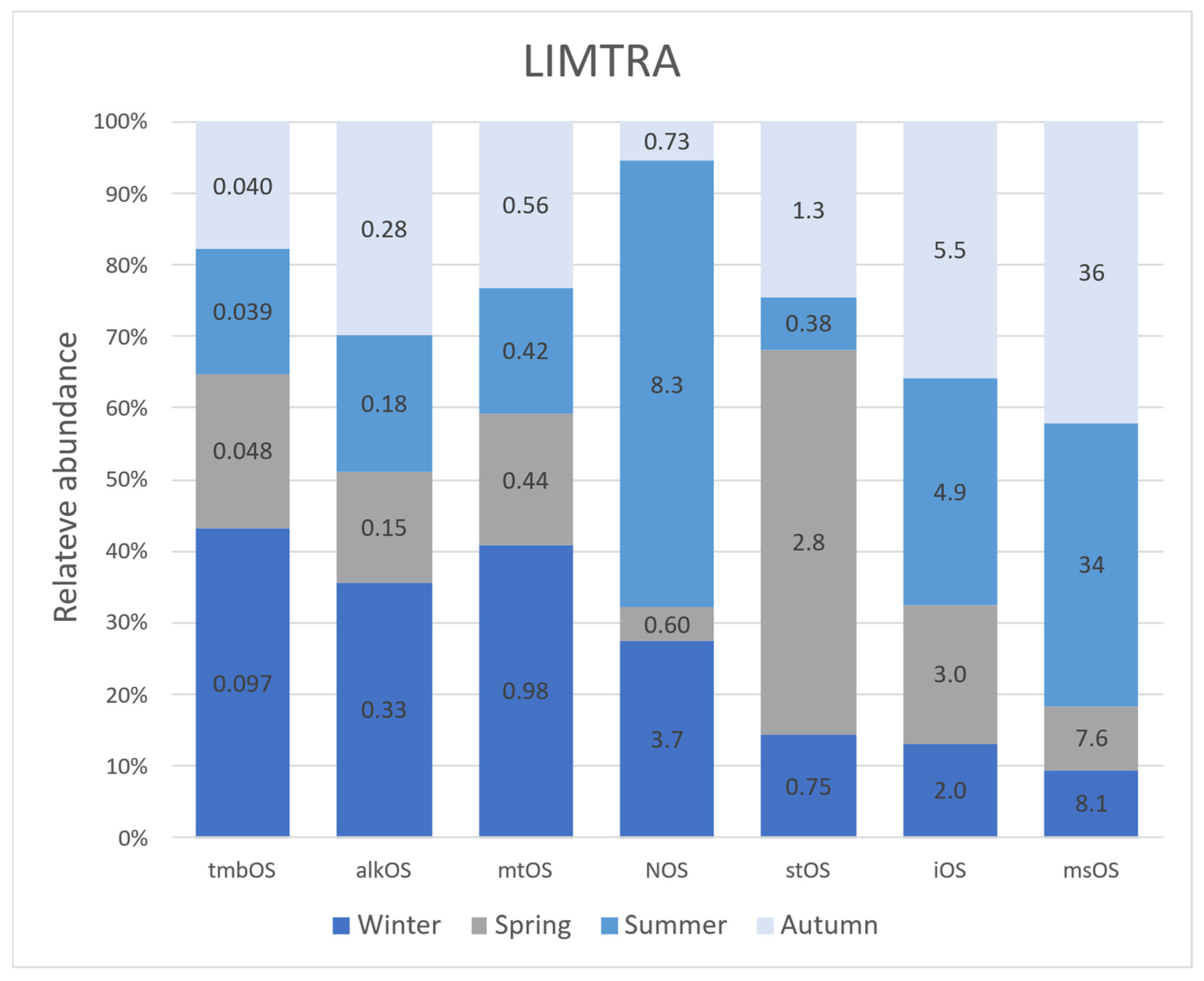
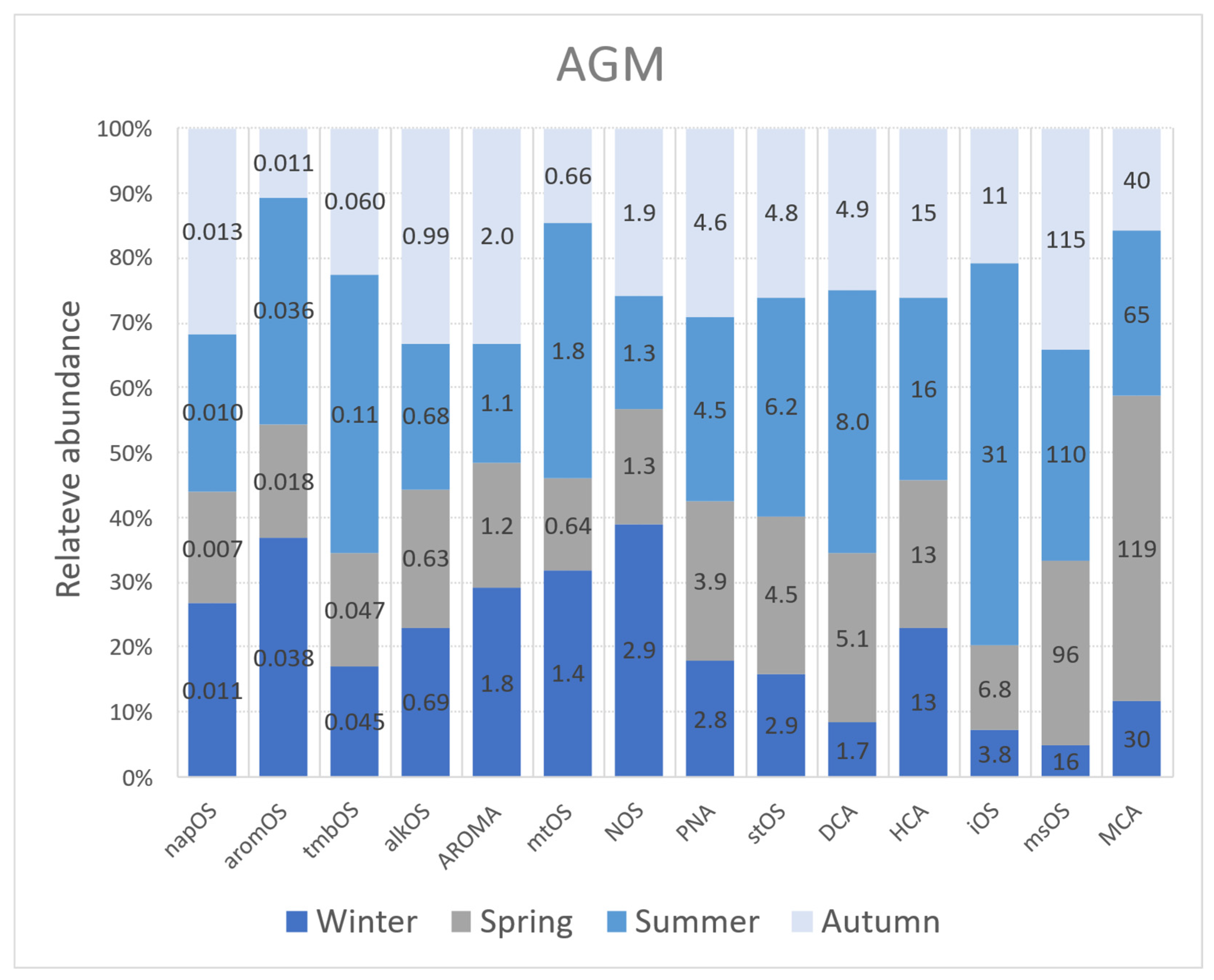
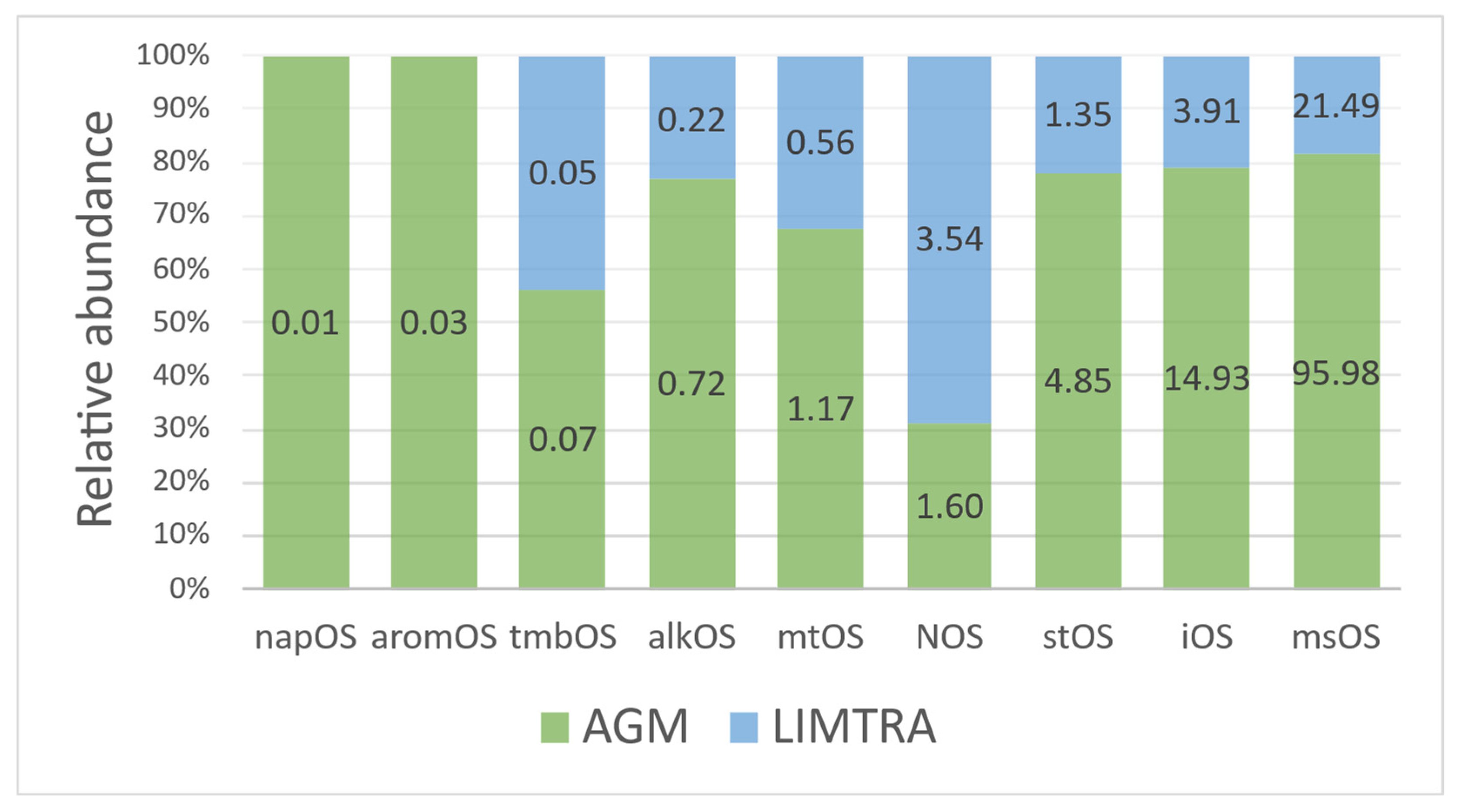
Figure 3 and Figure 4 show the seasonal relative abundance of each SOA group in 2019 at Limassol and Agia Marina respectively. Concerning the BSOAs, 82% and 67% of the annual msOS yield at Limassol and Agia Marina were detected during the warm period, respectively, which in Cyprus, consists of summer and autumn. Similarly, 68% and 80% of the annual iOS yield at Limassol and Agia Marina was detected during the warm period. The third most abundant group, NOSs, showed a relative abundance of 67% at Limassol for the same period; however, at Agia Marina, that percentage was 43%. At Limassol, the stOS levels were higher (68%) in the cold period, which in Cyprus, consists of winter and spring, while mtOS levels were nearly constant throughout the year and only slightly elevated during the cold period (59%). At Agia Marina, both stOS and mtOS levels were similar through the year.

Regarding the ASOAs, alkOS levels were relatively constant, exhibiting minimal seasonal variability at both stations. However, tmbOSs showed the opposite trends. At Limassol, the highest yield (65%) was found during the cold period, whereas at AGM, the warm period yield was 65% of the annual tmbOS load. AromOSs and napOSs were only measured at Agia Marina, where their levels appeared to be constant throughout the year; they reached their highest levels in winter (37%) and autumn (32%), respectively. As mentioned, only AGM samples were analyzed for organic acids. MCAs were most abundant (47%) during spring and DCAs were most abundant in summer (41%). The rest of the OA species (HCAs, PNAs, and AROMAs) showed constant levels.

4. Discussion

4.1. Seasonal Variation

Figure 3 shows the seasonal relative abundances of the SOA species at Limassol. In winter, we observed the presence of most of the OS groups, which showed significantly higher relative abundances compare to the other seasons. Although msOSs were clearly dominant (51%), the highest alkOS (2.1%), tmbOS (0.66%), mtOS (6.1%), and NOS (23%) loads also occurred in winter. This is a strong indication that they are of anthropogenic origin or that there is a strong anthropogenic influence on their formation processes, especially for terpenoids [18]. Other studies have argued fluctuations in terpene emissions are dependent on the plant of origin, relative humidity, temperature, and atmospheric oxidants [19], with some arguing that the yields are higher during cold periods especially in Eastern European and Mediterranean areas [20,21]. Furthermore, it has been reported that long-chain aliphatic alkanes and polyaromatic hydrocarbons, such as trimethylbenzenes, are emitted directly from industrial, farming, and shipping activities [22]. Urban traffic is also a source of SOA precursors, as well as high levels of nitrogen oxides, which contribute to nitro-oxysulfate formation. Finally, the high relative humidity levels and the low ambient temperature during this time can affect the volatility of organic compounds—which act as precursors—and SOA compounds and can facilitate their condensation to the particle liquid phase [23]. The other BSOA species, iOSs (13%) and stOSs (4.7%), were found in higher concentrations, but these levels are lower than the levels they display during the rest of the year. In spring, we observed similar trends for BSOAs, as the msOS (52%) and iOS (21%) levels were the same as those in winter. A significant increase in stOSs was observed. They constituted the third most abundant SOA (19%) in spring. This can be explained if we consider the origin of sesquiterpenes, which are precursors of OSs and are emitted from coniferous plants that bloom during spring in Cyprus’s climate [24]. The levels of mtOSs (3.0%), alkOSs (1.0%), and tmbOSs (0.33%) showed a decrease, possibly due to the higher temperature (average increase of 2.6 °C) and lower humidity levels (average decrease of 4.9%), which decreased the condensation rates [14,25]. NOSs were not detected at significant levels. During summer and autumn, the BSOAs dominated the SOA yield. The msOS, iOS, mtOS, and stOS groups accounted for 82% of the summer SOA yield and 98% of the autumn SOA yield, although mtOSs and stOSs were found at levels lower than those in the cold period. NOSs showed an important increase (17%) during summer, similar to the winter trend, but they decreased again to 1.6% during autumn. This increase could be explained by the intense tourism and increase in traffic and shipping that characterize the island during summer, activities that produce emissions that contribute to NOS formation. Less than 1% of the SOA yield was from alkOSs and tmbOSs during these seasons.

Similarly, at Agia Marina (Figure 4), winter was the season with the most SOA species showing significant levels. This season was dominated by MCAs (39%), followed by msOSs (21%) and HCAs (17%). Almost 5% of the SOA load was attributed to iOSs and almost 4% was attributed to stOSs, NOSs, and PNAs. The levels of these SOAs were the highest in winter, especially for NOSs, which then dropped to levels less than 1% of the total yield. DCAs, AROMAs, and mtOSs each constituted approximately 2% of the winter yield. Similar to NOSs, the winter yields of mtOSs and AROMAs were the highest; for the rest of the year, the contributions of these two groups decreased below 1% of the SOA yield. AlkOSs, tmbOSs, aromOSs, and napOSs accounted for less than 1% of the winter yield. The spring SOA levels behaved in a similar way. Seven species (napOSs, aromOSs, tmbOSs, alkOSs, AROMAs, mtOSs, and NOSs) each contributed to less than 1% and together accounted for 1.5%. PNA and stOS levels decreased to approximately 2% each, while DCA levels remained at the 2% they occupied in winter. HCA levels (5.2%) decreased to almost 1/3 of their winter yield and iOS levels (2.7%) decreased to half of their winter levels. The two dominant species, msOSs and MCAs, remained at their previous levels and continuing to have the highest yields of the season. Summer followed the same pattern with three major exceptions. Firstly, MCAs display a decrease, constituting 26% of SOAs and becoming the second most abundant species. The dominant species during summer was msOSs (45%) despite their summer mean not being the highest seasonal average. Secondly, iOSs show a significant increase, reaching 13% of the summer SOA yield. The same trend was observed during autumn: msOSs (57%) were the dominant group, followed by MCAs (20%) and iOSs (5.4%), while the same seven groups mentioned above continued to contribute less than 1% each, though their levels all increased and together they accounted for 3% of the total. Lastly, the tmbOSs exhibited an interesting trend as they increased by more than 50%. This is a typical behavior of BSOAs, indicating that they have common formation processes. It is also indicative of aerosol aging processes, suggesting that the longer lifetime of low-volatility SOAs allows them to be transported further from where they were generated. Notably, the levels of organic acids were also significantly high compared to those in other regions of the Mediterranean [17,26].

4.2. Spatial Variation

The different profiles of the two studied areas provide a unique opportunity for studying aerosol transport mechanisms, atmospheric aging processes, and pollutant residence times based on the results from the remote sampling site [27] and for assessing anthropogenically mediated SOA formation in coastal urban settings based on the results from the urban site [28]. In the spatial distribution study, in order to obtain reliable correlations between the two sites, we only included the samples collected on dates when sampling occurred at both sites. The November and December samples from Agia Marina were excluded from the dataset. Also, the spatial distribution only refers to OSs/ONs since the OAs in the LIMTRA samples were not measured.

The annual mean concentration of PM2.5 was 11.4 ± 5.0 μg∙m⁻³ at AGM (n = 70) and 21 ± 12 μg∙m⁻³ at LIMTRA (n = 69). In contrast, the total OS yield was higher in the AGM samples. As expected, msOSs, iOSs, mtOSs, and stOSs were found at higher levels at AGM. Their relative abundances and mean annual concentrations are displayed in Figure 5. Despite the known anthropogenic influence on alkOSs, their levels were also over three times higher at AGM; it was assumeding that the reason for this is that they might have a longer lifetime and can be transported from areas where anthropogenic emissions are high. Despite the aromOS and napOS yields (30 ± 20 pg∙m⁻³ and 10 ± 4 pg∙m⁻³, respectively) being significantly lower than those of any other OS species, they were only detected in the AGM samples, supporting the assumption of aerosol transportation. The most interesting observation was the opposite trend shown by the NOS group, which showed levels almost two times higher at LIMTRA. This underlines the anthropogenic effects on NOS formation, as NOSs are the most sensitive to anthropogenic emissions. Another possible explanation could be due to the NOS formation process, which is discussed in Section 4.3.2.

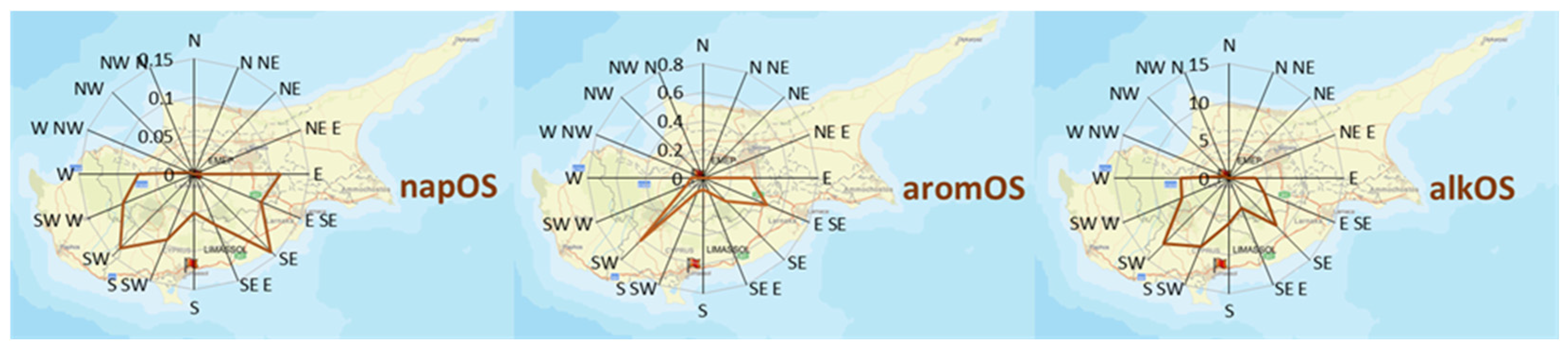
The elevated concentrations of alkOSs, tmbOSs, aromOSs, and napOSs, which are typically classified as anthropogenic SOAs, suggest influences from non-local emissions at the AGM site. The alignment of their distribution with south-southwest and southeast-east winds (Figure 6) indicates transport from urban/industrial regions. The eastern region includes Larnaca (which contains airport/port facilities) and Zygi (an industrial zone), whereas the southern region includes Pafos and Limassol (which contain airport/port facilities). These areas are characterized by heavy oil combustion and their emissions contain fossil fuel-derived VOCs like alkanes [29], BTEX [30], and PAHs [15], which may be oxidized during transport to form ASOAs. These results are consistent with the observed southeast wind-driven SOA gradients in Mediterranean coastal sites [31]. The persistence of these species in aerosols [32,33] further supports the long-range transport hypothesis.

4.3. Secondary Formation: Source Apportionment, SOA Correlations, and Atmospheric Oxidants’ Effect on Different Pathways

4.3.1. Positive Matrix Factorization

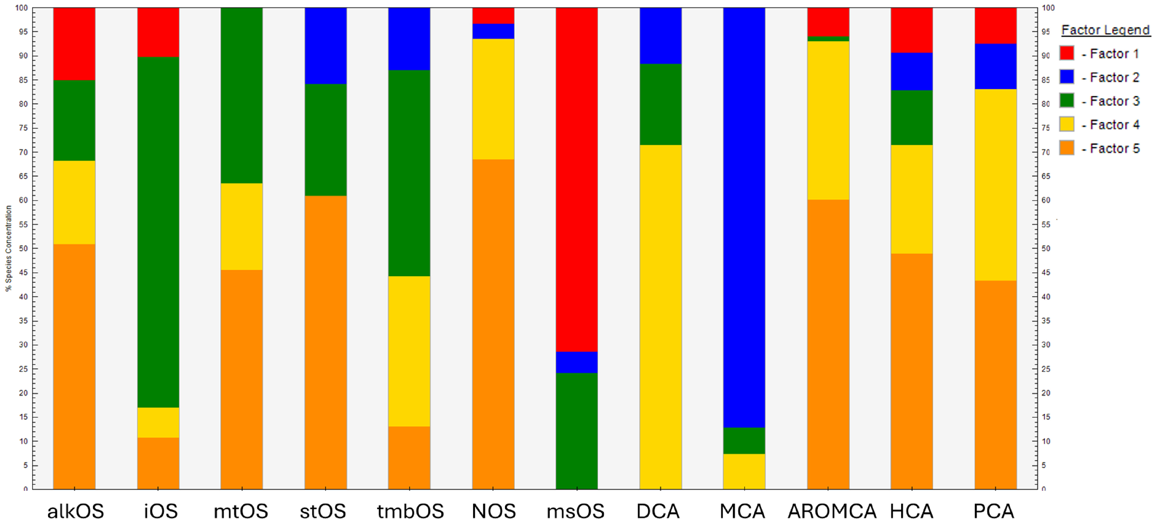
The contributions of the different SOA sources were investigated using the EPA’s Positive Matrix Factorization model (EPA PMF 5.0) and using the concentrations and uncertainties of 12 groups, including iOSs, mtOSs, stOSs, alkOSs, tmbOSs, NOSs, msOSs, DCAs, MCAs, AROMCAs, HCAs, and PNAs, as input. A total of 84 samples (after excluding outliers) were considered in the PMF model. The input matrix (84 × 12) adhered to the requirements for a statistically stable factor analysis. The uncertainties associated with the data were calculated according to the PMF User Guide [34]. Detailed information can be found in Appendix B. The number of factors was chosen considering the ratio of robust-to-theoretical parameters (QR/QT). To improve the quality of the profiles obtained, constraints were added. For the interpretation of the results and the apportionment of each factor, both the contributions of the species to each factor and the % percentage constitution of the species based on the five factors were taken into account (

Table A3. Contributions (%) of species to each factor.

	% of Factor Total
	Factor 1	Factor 2	Factor 3	Factor 4	Factor 5
alkOSs	0.18	0.00	0.35	0.80	2.70
iOSs	1.57	0.01	19.93	3.76	7.42
mtOSs	0.00	0.00	1.12	1.22	3.55
stOSs	0.00	0.57	1.72	0.00	11.43
tmbOSs	0.00	0.01	0.08	0.13	0.06
NOSs	0.08	0.07	0.00	2.45	7.71
msOSs	95.50	5.17	57.69	0.00	0.02
DCAs	0.01	0.90	2.70	25.06	0.00
MCAs	0.00	91.27	11.89	34.60	0.00
AROMCAs	0.14	0.00	0.05	2.97	6.29
HCAs	2.06	1.48	4.48	19.30	48.59
PNAs	0.47	0.51	0.00	9.73	12.23

and

Table A4. The % constitutions of the species based on the 5 factors.

	% of Species Sum
	Factor 1	Factor 2	Factor 3	Factor 4	Factor 5
alkOSs	15.00	0.00	16.70	17.30	50.90
iOSs	10.20	0.10	72.80	6.30	10.70
mtOSs	0.00	0.00	36.40	18.00	45.50
stOSs	0.00	15.80	23.20	0.00	61.00
tmbOSs	0.00	13.00	42.70	31.20	13.10
NOSs	3.30	3.20	0.00	25.10	68.50
msOSs	71.30	4.40	24.20	0.00	0.00
DCAs	0.10	11.50	16.90	71.50	0.00
MCAs	0.00	87.10	5.50	7.40	0.00
AROMCAs	5.90	0.00	1.10	32.80	60.20
HCAs	9.40	7.80	11.40	22.50	49.00
PNAs	7.50	9.50	0.00	39.80	43.30

, Appendix B). Specifically, the species with the higher yield in each factor was defined as the factor’s attribution to a potential source, while the variability in the species defined the total abundance of a factor to provide insights beyond the source and correlate the factor with specific formation pathways.

Figure 7 presents the 5 Factor Profiles, resulted from PMF. Factor 1 was defined by msOSs (95.5%) and the highest alkOS (15%) and iOS (10.2%) yields. Based on similar findings ([35,36]), the three OS species were characterized as isoprene oxidation products via oxidation of IEPOXY-diols. Thus, Factor 1 was attributed to “isoprene oxidation”. The formation mechanisms of most of these species are known to be driven by ozone levels, as discussed in Section 4.3.2, and this could explain the loadings of AROMCAs, HCAs, and PNAs in Factor 1.

Similarly, Factor 2 was defined by MCAs (91.3%) and contributed to stOSs (15.8%), tmbOSs (13.0%), and DCAs (11.5%). Since MCAs have been associated with emissions from burning biomass [37], Factor 2 can be attributed to “biomass burning”. High-molecular-weight DCAs have been also found to derive from biogenic sources in other studies [38]. It is interesting to note that, to date, there is little evidence that stOSs and tmbOSs are emitted or instantly formed on site during BB [39]. However, stOSs are products of sesquiterpenes found in plants and living organisms, mainly marine organisms and fungi, which have lower volatility than monoterpenes; thus, it is possible that they are also present in biomass stocks, especially in coastal areas. Aromatic compounds, such as trimethylbenzene, have also been found in BB emissions.

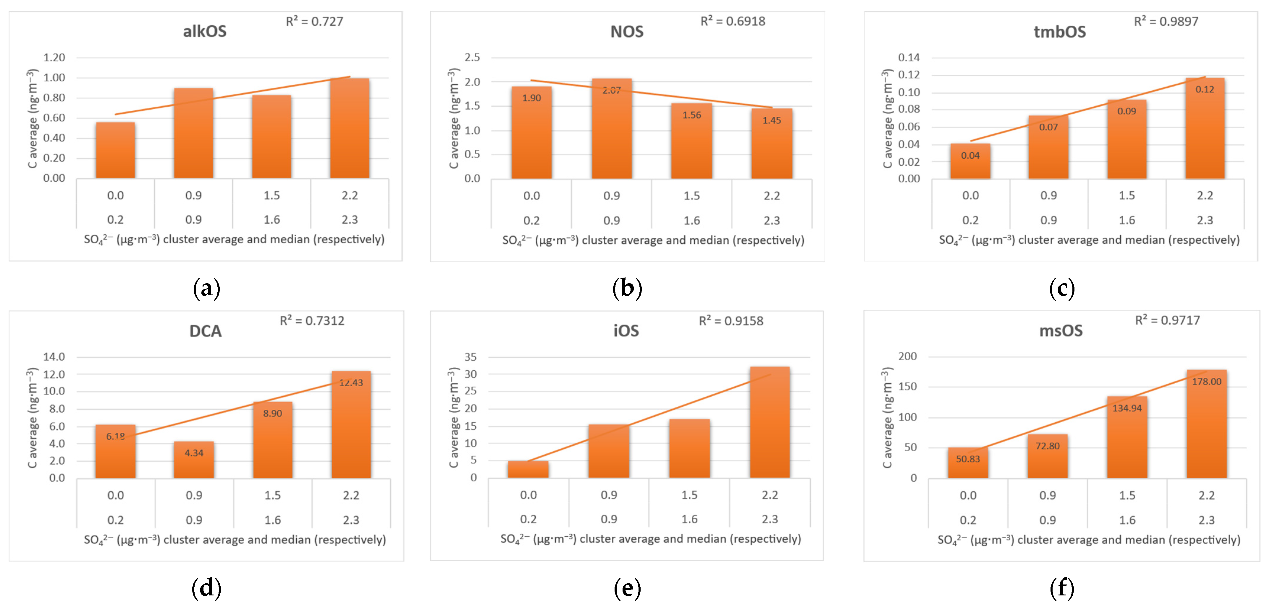
Factor 3 was the first factor showing a higher variability in its defining groups. The msOSs (48.6%) had the highest contribution to the factor profile, followed by DCAs (20.4%). Μost of the OS groups had high contributions to Factor 3: iOSs (72.8%), tmbOSs (42.7%), mtOSs (36.4%), msOSs (24.2%), stOSs (23.2%), and alkOSs (16.7%). In addition, most of these species’ normalized concentrations exhibited a high correlation (R² > 0.7) with SO₄²⁻ levels (Figure 8), similar to the findings previously reported in [40] where SOA products of methyltetrols were weakly correlated with aerosol acidity and SO₄²⁻ level. DCAs had a comparable contribution to Factor 3 (16.9%) and showed a high correlation (R² > 0.7) with SO₄²⁻ levels as well, which indicates that some DCAs, especially the low-molecular-weight ones, could be second-generation oxidation products. In conclusion, we attributed Factor 3 to “second-generation SOA formation” via sulfur oxides. It is notable that NOSs, the only organosulfate group remaining from those studied, did not contribute to Factor 3, nor did it correlate with SO₄²⁻ levels; on the contrary, it showed a negative correlation, indicating a different formation pathway and a negative effect of aerosol acidity on the formation of organonitrate compounds. This intriguing finding could indicate a strong effect of NO₃ radical chemistry and possible competition with sulphate pathways. N. L. Ng et al. [41] have already highlighted that nitrate radical reactions can compete with hydroxyl radical reactions, especially for multifunctional compounds and during night time when photochemistry as the main source of OH∙ is less important.

Factor 4 was also dependent on multiple groups, similar to Factor 3. It was mostly defined by MCAs (34.6%), as well as DCAs (25.1%) and HCAs (19.3%). Similar to Factor 3, most of the organic acid groups showed high contributions to this factor: DCAs (71.5%), PNAs (39.8%), AROMCAs (32.8%), and HCAs (22.5%). Organic acids have been generally characterized as first-generation SOA species, so Factor 4 was attributed to “first-generation SOA formation”. The fact that the factor is defined by MCAs shows that they are precursor compounds, which are transformed to DCAs through various oxidation processes. HCAs have been known to act as chain-reaction intermediates in the production of high-molecular-weight DCAs from MCAs, especially the unsaturated ones ([42,43]). This hypothesis is strongly supported by the contribution of each species to the factor. Furthermore, PNAs as well as AROMCAs were correlated with Factor 4 and although they are believed to have different precursors, this is an indication that they can form during primary organic aerosol formation. In general, Factors 3 and 4 could be indicative of aerosol aging, assuming that Factor 3 refers to the second stage of aging of aerosol sulphates and photocatalysis when exposed to sunlight, and Factor 4 refers to the first stage of aging through oxidation processes, which mostly depends on the atmospheric oxidant levels.

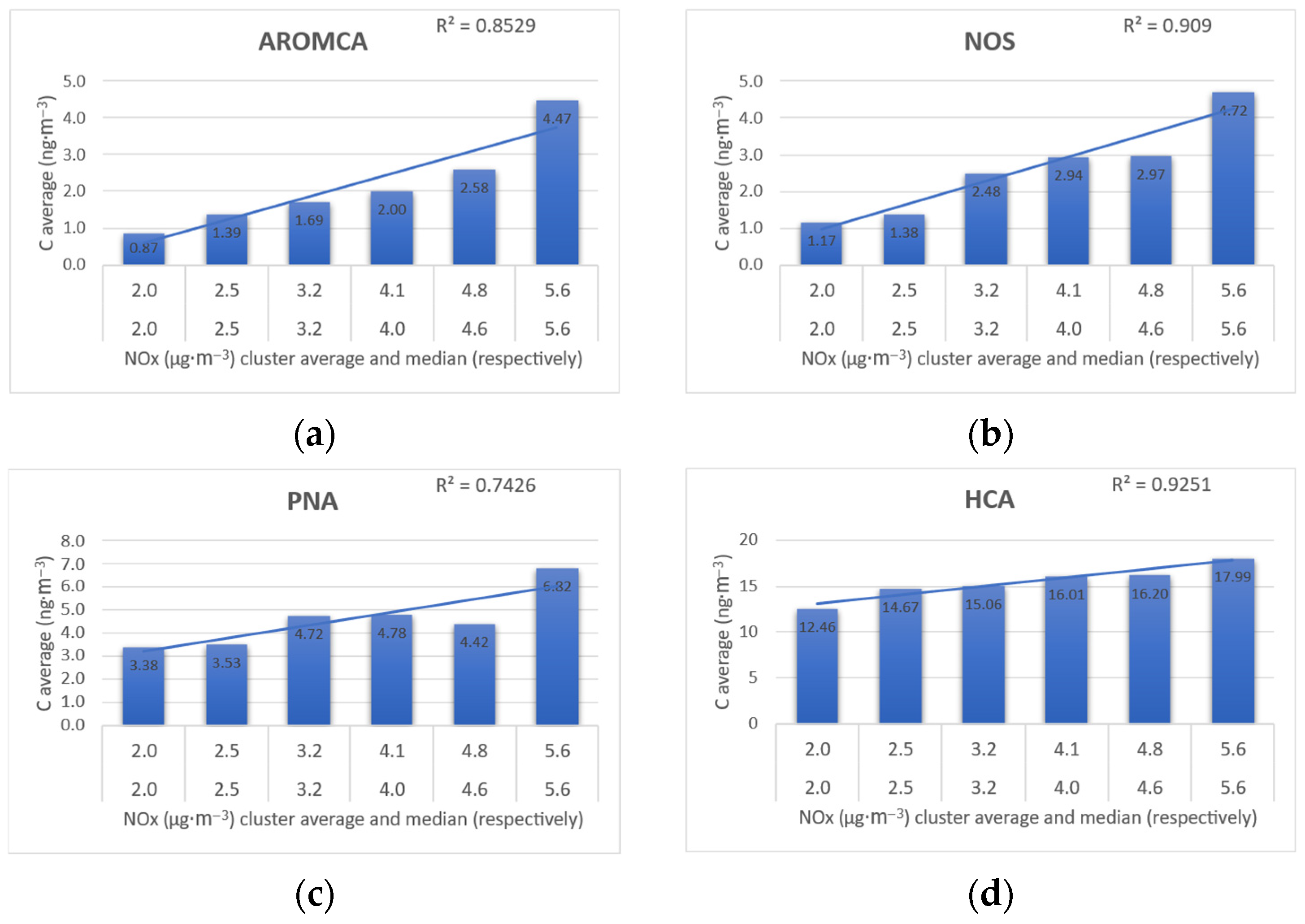
Finally, Factor 5 was defined by HCAs (48.6%) and PNAs (12.2%), and it has high contributions from NOSs (68.5%), AROMCAs (60.2%), HCAs (49.0%), and PNAs (43.3%). The contributions of HCAs and PNAs to the factor indicates that the oxidation of pinenes could be the source. In previous studies [15,44], pinene-oxidation markers have been paired with isoprene-oxidation markers and correlated with high NO_x levels. Therefore, we assessed the correlation of all the species connected to this factor with NO_x levels. All correlation coefficients were found to be statistically significant (R² > 0.7) (Figure 9), providing evidence for the formation of the aforementioned groups through nitrogen oxide pathways. So, we attributed Factor 5 to “pinene oxidation” via nitrogen oxides. The proposal that pinene–NO_x interactions lead to the formation of HCAs and PNAs is supported by recent literature [45].

4.3.2. Principal Component Analysis

The five factors, presented in

Table 3. Varimax rotated component matrix for the SOA species.

Rotated Component Matrix a
Variance (%)	27	15	14	11	10
Factor	1	2	3	4	5
alkOSs	0.262	0.134	−0.055	0.833	0.033
iOSs	0.884	0.218	−0.008	0.154	0.059
msOSs	0.777	−0.227	−0.018	0.108	0.131
mtOSs	0.321	0.854	0.029	0.061	−0.158
NOSs	−0.303	0.738	0.220	0.245	0.182
stOSs	−0.020	0.111	0.068	0.138	0.840
tmbOSs	0.708	0.567	0.126	0.004	0.180
AROMCAs	−0.038	0.190	0.709	0.542	−0.155
DCAs	0.759	0.128	0.439	−0.052	0.019
MCAs	0.318	−0.160	−0.015	−0.292	0.596
HCAs	0.605	−0.012	0.511	0.171	−0.040
PNAs	0.182	0.101	0.795	−0.233	0.181

^a Extraction Method: Principal Component Analysis. Rotation Method: Varimax with Kaiser Normalization.

, explained 68% of the total variance; the lowest factor score was 0.5.

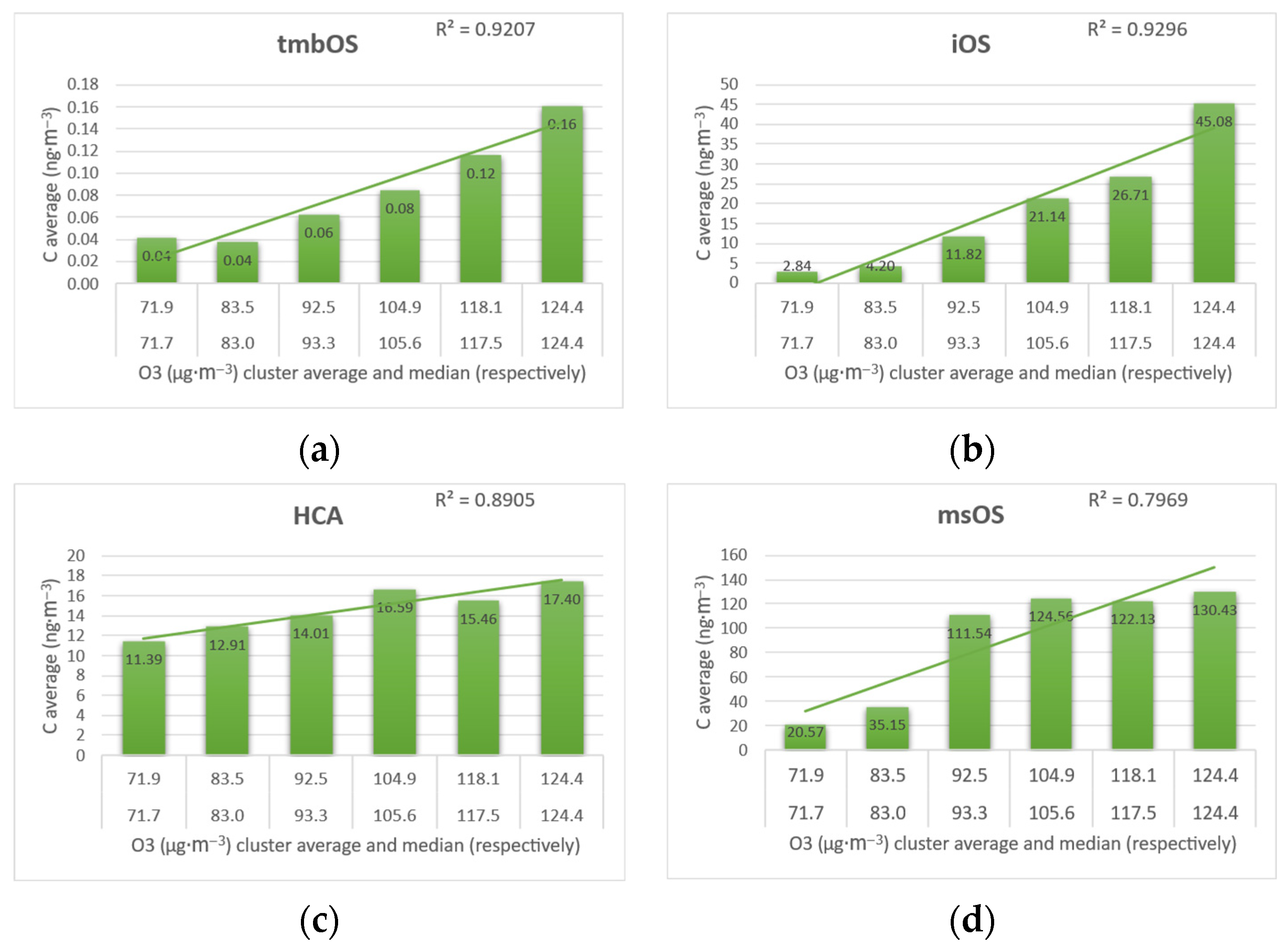
Factor 1 (27% of the variance) was loaded with mostly biogenically derived SOAs, like iOSs, msOSs, DCAs, and HCAs. On the other hand, the groups that were the least influenced by anthropogenic emissions, like tmbOSs, show high yields for the first factor. Therefore, Factor 1 was not affected by a specific source. We further investigated the formation pathways that these species may follow. We normalized the SOA levels based on the inorganic gases acting as atmospheric oxidants (nitrogen oxides and ozone), as well as sulfur dioxide that contributes to aerosol acidity and consequently to transformation processes. We found that these specific groups showed strong correlations (R² > 0.5) with ozone levels, pointing to a specific formation pathway (Figure 10). As a result, Factor 1 was associated with “oxidation processes via ozone”. Other studies have reported similar observations of O₃ correlations with BSOAs in forested regions [46]. We observed high correlations between MCA and ozone levels as well, although they did not have a high loading for Factor 1. On the contrary, their highest loading was for Factor 4 so they will be discussed later. Interestingly, DCAs did not show high correlation with ozone levels. In fact, the DCAs were most abundant when ozone levels were at their lowest, although they increased proportionally to O₃, from approximately 80 μg∙m⁻³ of ozone. This can be an indicator that DCAs are intermediates in the formation of other SOAs. At relatively low ozone levels, primary emissions can form DCAs, which then undergo similar processes to form second-generation SOAs. This is consistent with Factor 3 from the PMF analysis.

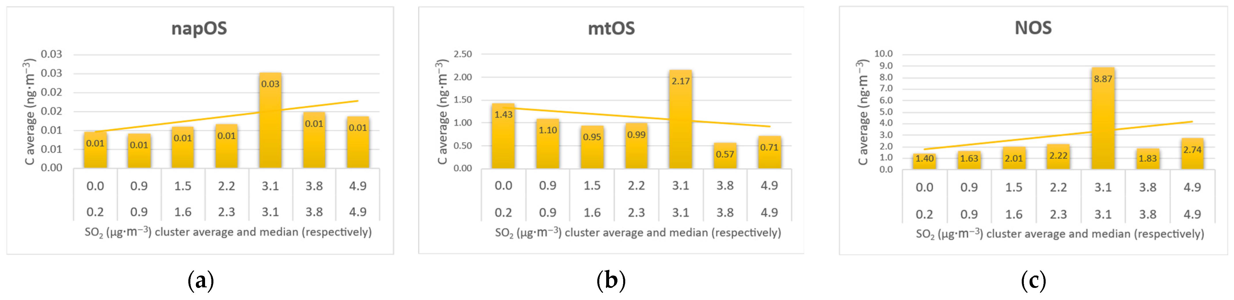
Factor 2 was tightly clustered with mtOSs, NOSs, and also tmbOSs, which showed a loading similar to that for Factor 1. These groups are generally considered to be anthropogenically derived, although they are not known to have the same precursors, nor do they have a common oxidation process. By examining the normalized data, we found that they share a common influence: sulfur dioxide (SO₂). There have been numerous reports in the recent literature concerning the influence of SO₂ on aerosol acidity and if it affects SOA formation. The reports are highly controversial and to this day, there is no a clear consensus. Jiang et al. found strong correlations between OSs and SO₂ in chamber experiments and they also identified OSs in field samples. H. O. T. Pye et al. [47] also pointed out the importance of SO₂ in SOA formation, stating that the promoting effect of SO₂ might be related to the increase in particle acidity. The chamber experiments that they performed showed that increasing the SO₂ concentration seemed to benefit SOA formation under both high and low NO_x conditions. According to our observations, a certain sulfur dioxide level prompts OS formation (Figure 11). At the level of 3.1 μg∙m⁻³ of SO₂, there was a spike of aromatic and nitro-oxy organosulfates that was not observed for any other group. Bougiatioti et al. [14], also pointed out a specific SO₂ level of 2 μg∙m⁻³ as the optimal concentration for SOA formation in a Mediterranean area. It is possible that lower concentrations of SO₂ do not promote SOA formation, whereas at higher levels, the particle acidity might cause further aerosol transformation. Yang et al. also found that the abundances of relatively low-molecular-weight compounds (m/z < 200) decreased in experiments when SO₂ was added, indicating that the presence of SO₂ may promote oligomer formation in the particle phase. Thus, Factor 2 was attributed to “aerosol acidity due to the presence of SO₂”. Some studies have argued that SOA levels are suppressed by SO₂ because it competes for oxidants [32]. This study’s findings strongly support the catalytic action of SO₂. It is possible that NO_x and O₃ act synergistically and mediate the interaction of SO₂ and aerosol compounds to enhance a particular oxidation pathway involved in aerosol aging.

Factor 3 was loaded with dicarboxylic and pinic-related organic acids, which could be direct emissions rather than produced SOAs. They are known to derive from plant emissions so we attributed this factor to “biogenic sources”. This factor has similarities with Factor 4 from the PMF analysis, but it has fewer group loadings and therefore cannot statistically support the first-generation SOA assumption.

Factor 4 correlated with two groups: alkOSs and AROMAs, which showed stable levels throughout the year, i.e., did not show seasonal trends, and are believed to mainly derive from “anthropogenic sources”. AROMA levels were highly correlated with NO_x levels in the atmosphere (R² = 0.850 for normalized concentrations of AROMAs based on NO_x levels). The correlation between nitrogen oxides and alkOSs was not as significant at AGM (R² = 0.13), but they were highly correlated at LIMTRA (R² = 0.70) and in other studies as well. This is not surprising since aromatic compounds are more stable and have a longer lifetime. Their subsequent oxidation after they were transported away from where they were emitted (city centers) was affected by the NO_x levels at AGM. On the other hand, the alkOSs detected at AGM may have formed close to their emission site so they were not correlated with NO_x levels.

Factor 5 seems to be correlated with high-molecular-weight C16-C18 organic monocarboxylic acids. They displayed unique seasonal distributions, with their highest levels occurring in spring. They are of biogenic origin and they appear to be highly correlated with O₃ levels, indicating that ozone is the main oxidant in their formation process. However, their levels are strongly influenced by anthropogenic activity like biomass burning, cooking, and burning fuel. Therefore, they had much higher yields compared to the other SOA species that define Factor 1. Also, they reach their highest levels during the cold period, unlike the other species. The strong “anthropogenic influence of biogenic emissions” is believed to differentiate MCAs and define Factor 5. These findings agree with those of the PMF analysis, where Factor 2 correlated MCAs and stOSs.

5. Conclusions and Future Perspectives

A total of 118 compounds from 14 different SOA groups were identified in PM2.5 samples collected from Limassol, an urban/traffic site, and Agia Marina, a remote EMEP station, on Cyprus during a 1-year period in 2019. The two areas displayed different profiles, with AGM having the highest levels of SOA compounds on average. In the AGM PM samples, the most abundant SOAs were msOSs, MCAs, and iOSs, forming the profile of a biogenically-derived aerosol; several anthropogenically derived aromatic compounds were also detected at low levels. At the LIMTRA station, msOSs and iOSs exhibited the highest levels, but the presence of alkOSs, mtOSs, tmbOSs, and NOSs indicated a more human-induced profile. The main finding was the higher yield of NOSs at LIMTRA than at AGM, which highlights the traffic levels of these areas. The most interesting findings was the presence of aromatic sulfates only at the remote station, which indicates that they have a longer lifetime and are transported long distances from their emission/formation site. Seasonal trends were also studied. AGM SOA levels reached an annual maximum in spring, possibly due to increased biogenic emissions from plants in the nearby forested areas. LIMTRA SOA levels were at their highest in summer, which is related to higher temperatures, ozone levels, and perhaps more intense shipping activities.

This study employed PMF and PCA to elucidate the sources and formation pathways of the OSs, ONs, and OAs in PM2.5, revealing complex interactions between biogenic precursors, anthropogenic emissions, and atmospheric chemistry. PMF resolved five factors: (1) isoprene oxidation (dominated by msOSs, alkOSs, and iOSs, and linked to IEPOX pathways and O₃-driven chemistry), (2) biomass burning (dominated by MCAs and stOSs; trimethylbenzene derivatives suggest a coastal biogenic influence), (3) second-generation SOA formation (sulfate-driven; high OS–DCA correlation implicates SO₄²⁻ in aging processes), (4) first-generation SOA formation (oxidation of MCAs to DCAs via HCA intermediates), and (5) pinene oxidation via NO_x (HCA/PNA formation under high NO_x conditions). Notably, NOS levels exhibited a negative correlation with atmospheric sulfate levels, underscoring competition between nitrate and sulfate radical pathways. The PCA corroborated the PMF results’ biogenic/anthropogenic distinctions but emphasized oxidative processes: Factor 1 was linked OSs/DCAs to O₃ while Factor 2 correlated mtOSs/NOSs with SO₂-driven aerosol acidity, revealing a catalytic threshold (~3.1 μg∙m⁻³) for OS formation. Factor 5 highlighted hybrid anthropogenic–biogenic signals (e.g., combustion influences MCA seasonality). Divergences in source resolution were determined to be contributions by PMF, whereas PCA identified covariance patterns but lacked mechanistic specificity. The most notable findings of the study were the dual roles of SO₂ in promoting OS formation at moderate levels but suppressing it at higher concentrations due to oxidant competition. In addition, the NO_x-O₃ synergy in the formation of pinene-derived and isoprene-derived SOAs reflects competing oxidation paths. The PMF factor profiles provided explicit source apportionment, while the PCA uncovered latent relationships (SO₂ catalysis); however, these relationships require auxiliary data (gas-phase correlations) to interpret them. This multi-tracer, multi-method approach advances SOA research by disentangling precursor–source–pathway dynamics in polluted environments.

References

1. Mahilang, M.; Deb, M.K.; Pervez, S. Biogenic secondary organic aerosols: A review on formation mechanism, analytical challenges and environmental impacts. Chemosphere 2021, 262, 127771. [Google Scholar] [CrossRef] [PubMed]
2. Klyta, J.; Czaplicka, M. Determination of secondary organic aerosol in particulate matter—Short review. Microchem. J. 2020, 157, 104997. [Google Scholar] [CrossRef]
3. Hallquist, M.; Wenger, J.C.; Baltensperger, U.; Rudich, Y.; Simpson, D.; Claeys, M.; Dommen, J.; Donahue, N.M.; George, C.; Goldstein, A.H.; et al. The formation, properties and impact of secondary organic aerosol: Current and emerging issues. Atmos. Chem. Phys. 2009, 9, 5155–5236. [Google Scholar] [CrossRef]
4. Kalkavouras, P.; Bougiatioti, A.; Grivas, G.; Stavroulas, I.; Kalivitis, N.; Liakakou, E.; Gerasopoulos, E.; Pilinis, C.; Mihalopoulos, N. On the regional aspects of new particle formation in the Eastern Mediterranean: A comparative study between a background and an urban site based on long term observations. Atmos. Res. 2020, 239, 104911. [Google Scholar] [CrossRef]
5. Wang, W.; Zhang, Y.; Cao, G.; Song, Y.; Zhang, J.; Li, R.; Zhao, L.; Dong, C.; Cai, Z. Influence of COVID-19 lockdown on the variation of organic aerosols: Insight into its molecular composition and oxidative potential. Environ. Res. 2022, 206, 112597. [Google Scholar] [CrossRef]
6. Serafeim, E.; Besis, A.; Kouras, A.; Farias, C.N.; Yera, A.B.; Pereira, G.M.; Samara, C.; de Castro Vasconcellos, P. Oxidative potential of ambient PM2.5 from São Paulo, Brazil: Variations, associations with chemical components and source apportionment. Atmos. Environ. 2023, 298, 119593. [Google Scholar] [CrossRef]
7. Paraskevopoulou, D.; Bougiatioti, A.; Stavroulas, I.; Fang, T.; Lianou, M.; Liakakou, E.; Gerasopoulos, E.; Weber, R.; Nenes, A.; Mihalopoulos, N. Yearlong variability of oxidative potential of particulate matter in an urban Mediterranean environment. Atmos. Environ. 2019, 206, 183–196. [Google Scholar] [CrossRef]
8. Khan, F.; Kwapiszewska, K.; Zhang, Y.; Chen, Y.; Lambe, A.T.; Kołodziejczyk, A.; Jalal, N.; Rudzinski, K.; Martínez-Romero, A.; Fry, R.C.; et al. Toxicological Responses of α-Pinene-Derived Secondary Organic Aerosol and Its Molecular Tracers in Human Lung Cell Lines. Chem. Res. Toxicol. 2021, 34, 817–832. [Google Scholar] [CrossRef]
9. Bimenyimana, E.; Pikridas, M.; Oikonomou, K.; Iakovides, M.; Christodoulou, A.; Sciare, J.; Mihalopoulos, N. Fine aerosol sources at an urban background site in the Eastern Mediterranean (Nicosia; Cyprus): Insights from offline versus online source apportionment comparison for carbonaceous aerosols. Sci. Total Environ. 2023, 893, 164741. [Google Scholar] [CrossRef]
10. Wang, Y.; Chen, Y.; Wu, Z.; Shang, D.; Bian, Y.; Du, Z.; H. Schmitt, S.; Su, R.; I. Gkatzelis, G.; Schlag, P.; et al. Mutual promotion between aerosol particle liquid water and particulate nitrate enhancement leads to severe nitrate-dominated particulate matter pollution and low visibility. Atmos. Chem. Phys. 2020, 20, 2161–2175. [Google Scholar] [CrossRef]
11. Kristensen, K.; Glasius, M. Organosulfates and oxidation products from biogenic hydrocarbons in fine aerosols from a forest in North West Europe during spring. Atmos. Environ. 2011, 45, 4546–4556. [Google Scholar] [CrossRef]
12. Glasius, M.; Thomsen, D.; Wang, K.; Iversen, L.S.; Duan, J.; Huang, R.J. Chemical characteristics and sources of organosulfates, organosulfonates, and carboxylic acids in aerosols in urban Xi’an, Northwest China. Sci. Total Environ. 2022, 810, 151187. [Google Scholar] [CrossRef]
13. King, A.C.F.; Giorio, C.; Wolff, E.; Thomas, E.; Karroca, O.; Roverso, M.; Schwikowski, M.; Tapparo, A.; Gambaro, A.; Kalberer, M. A new method for the determination of primary and secondary terrestrial and marine biomarkers in ice cores using liquid chromatography high-resolution mass spectrometry. Talanta 2019, 194, 233–242. [Google Scholar] [CrossRef]
14. Bougiatioti, A.; Nikolaou, P.; Stavroulas, I.; Kouvarakis, G.; Weber, R.; Nenes, A.; Kanakidou, M.; Mihalopoulos, N. Particle water and pH in the eastern Mediterranean: Source variability and implications for nutrient availability. Atmos. Chem. Phys. 2016, 16, 4579–4591. [Google Scholar] [CrossRef]
15. Yu, S.S.; Jia, L.; Xu, Y.F.; Pan, Y.P. Molecular composition of secondary organic aerosol from styrene under different NOx and humidity conditions. Atmos. Res. 2022, 266, 105950. [Google Scholar] [CrossRef]
16. Kanellopoulos, P.G.; Verouti, E.; Chrysochou, E.; Koukoulakis, K.; Bakeas, E. Primary and secondary organic aerosol in an urban/industrial site: Sources, health implications and the role of plastic enriched waste burning. J. Environ. Sci. 2021, 99, 222–238. [Google Scholar] [CrossRef] [PubMed]
17. Kanellopoulos, P.G.; Kotsaki, S.P.; Chrysochou, E.; Koukoulakis, K.; Zacharopoulos, N.; Philippopoulos, A.; Bakeas, E. PM2.5-bound organosulfates in two Eastern Mediterranean cities: The dominance of isoprene organosulfates. Chemosphere 2022, 297, 134103. [Google Scholar] [CrossRef]
18. Wang, Y.; Ma, Y.; Li, X.; Kuang, B.Y.; Huang, C.; Tong, R.; Yu, J.Z. Monoterpene and Sesquiterpene α-Hydroxy Organosulfates: Synthesis, MS/MS Characteristics, and Ambient Presence. Environ. Sci. Technol. 2019, 53, 12278–12290. [Google Scholar] [CrossRef]
19. Malik, T.G.; Sahu, L.K.; Gupta, M.; Mir, B.A.; Gajbhiye, T.; Dubey, R.; Clavijo McCormick, A.; Pandey, S.K. Environmental Factors Affecting Monoterpene Emissions from Terrestrial Vegetation. Plants 2023, 12, 3146. [Google Scholar] [CrossRef]
20. Copolovici, L.; Kännaste, A.; Pazouki, L.; Niinemets, Ü. Emissions of green leaf volatiles and terpenoids from Solanum lycopersicum are quantitatively related to the severity of cold and heat shock treatments. J. Plant Physiol. 2012, 169, 664–672. [Google Scholar] [CrossRef]
21. Byron, J.; Kreuzwieser, J.; Purser, G.; van Haren, J.; Ladd, S.N.; Meredith, L.K.; Werner, C.; Williams, J. Chiral monoterpenes reveal forest emission mechanisms and drought responses. Nature 2022, 609, 307–312. [Google Scholar] [CrossRef]
22. Jiang, H.; He, Y.; Wang, Y.; Li, S.; Jiang, B.; Carena, L.; Li, X.; Yang, L.; Luan, T.; Vione, D.; et al. Formation of organic sulfur compounds through SO2-initiated photochemistry of PAHs and dimethylsulfoxide at the air-water interface. Atmos. Chem. Phys. 2022, 22, 4237–4252. [Google Scholar] [CrossRef]
23. Liu, S.; Liu, X.; Wang, Y.; Zhang, S.; Wu, C.; Du, W.; Wang, G. Effect of NOx and RH on the secondary organic aerosol formation from toluene photooxidation. J. Environ. Sci. 2022, 114, 1–9. [Google Scholar] [CrossRef] [PubMed]
24. Kleist, E.; Mentel, T.F.; Andres, S.; Bohne, A.; Folkers, A.; Kiendler-Scharr, A.; Rudich, Y.; Springer, M.; Tillmann, R.; Wildt, J. Irreversible impacts of heat on the emissions of monoterpenes, sesquiterpenes, phenolic BVOC and green leaf volatiles from several tree species. Biogeosciences 2012, 9, 5111–5123. [Google Scholar] [CrossRef]
25. Amaladhasan, D.A.; Heyn, C.; Hoyle, C.R.; El Haddad, I.; Elser, M.; Pieber, S.M.; Slowik, J.G.; Amorim, A.; Duplissy, J.; Ehrhart, S.; et al. Modelling the gas-particle partitioning and water uptake of isoprene-derived secondary organic aerosol at high and low relative humidity. Atmos. Chem. Phys. 2022, 22, 215–244. [Google Scholar] [CrossRef]
26. Chazeau, B.; El Haddad, I.; Canonaco, F.; Temime-Roussel, B.; D’Anna, B.; Gille, G.; Mesbah, B.; Prévôt, A.S.H.; Wortham, H.; Marchand, N. Organic aerosol source apportionment by using rolling positive matrix factorization: Application to a Mediterranean coastal city. Atmos. Environ. X 2022, 14, 100176. [Google Scholar] [CrossRef]
27. Jimenez, J.L.; Canagaratna, M.R.; Donahue, N.M.; Prevot, A.S.H.; Zhang, Q.; Kroll, J.H.; DeCarlo, P.F.; Allan, J.D.; Coe, H.; Ng, N.L.; et al. Evolution of organic aerosols in the atmosphere. Science 2009, 326, 1525–1529. [Google Scholar] [CrossRef]
28. Hu, J.; Wang, P.; Ying, Q.; Zhang, H.; Chen, J.; Ge, X.; Li, X.; Jiang, J.; Wang, S.; Zhang, J.; et al. Modeling biogenic and anthropogenic secondary organic aerosol in China. Atmos. Chem. Phys. 2017, 17, 77–92. [Google Scholar] [CrossRef]
29. Qi, A.; Lv, J.; Wang, Y.; Wang, P.; Tuo, X.; Yang, L.; Wang, W. Distributions, spatial patterns and source identification of n-alkanes in air and bulk deposition in the eastern coastal areas of China: Fluxes and removal efficiency of bulk deposition. Atmos. Pollut. Res. 2024, 15, 102083. [Google Scholar] [CrossRef]
30. Ghahri, A.; Seydi, P.; Ranjbar, A.; Hatami, H.; Beheshti, T.; Seydi, E. Evaluation of exposure to volatile organic compounds (BTEX) and Polycyclic Aromatic Hydrocarbons (PAHs) in gas station workers and oxidative stress assessment in Karaj city. Toxicol. Rep. 2024, 13, 101767. [Google Scholar] [CrossRef]
31. Pikridas, M.; Vrekoussis, M.; Sciare, J.; Kleanthous, S.; Vasiliadou, E.; Kizas, C.; Savvides, C.; Mihalopoulos, N. Spatial and temporal (short and long-term) variability of submicron, fine and sub-10 μm particulate matter (PM1, PM2.5, PM10) in Cyprus. Atmos. Environ. 2018, 191, 79–93. [Google Scholar] [CrossRef]
32. Liu, J.; Zhu, S.; Guo, T.; Jia, B.; Xu, L.; Chen, J.; Cheng, P. Smog chamber study of secondary organic aerosol formation from gas- and particle-phase naphthalene ozonolysis. Atmos. Environ. 2023, 294, 119490. [Google Scholar] [CrossRef]
33. Tao, S.; Lu, X.; Levac, N.; Bateman, A.P.; Nguyen, T.B.; Bones, D.L.; Nizkorodov, S.A.; Laskin, J.; Laskin, A.; Yang, X. Molecular characterization of organosulfates in organic aerosols from Shanghai and Los Angeles urban areas by nanospray-desorption electrospray ionization high-resolution mass spectrometry. Environ. Sci. Technol. 2014, 48, 10993–11001. [Google Scholar] [CrossRef] [PubMed]
34. Norris, G. Duvall Rachelle EPA Positive M Atrix Factorization (PM F) 5.0 Fundamentals and User Guide; U.S. Environmental Protection Agency: National Exposure Research Laboratory, Research Triangle Park, NC, and Office of Research and Development: Washington, DC, USA, 2014. [Google Scholar]
35. Nestorowicz, K.; Jaoui, M.; Jan Rudzinski, K.; Lewandowski, M.; Kleindienst, T.E.; Spólnik, G.; Danikiewicz, W.; Szmigielski, R. Chemical composition of isoprene SOA under acidic and non-acidic conditions: Effect of relative humidity. Atmos. Chem. Phys. 2018, 18, 18101–18121. [Google Scholar] [CrossRef]
36. Zhang, J.; Shrivastava, M.; Zelenyuk, A.; Zaveri, R.A.; Surratt, J.D.; Riva, M.; Bell, D.; Glasius, M. Observationally Constrained Modeling of the Reactive Uptake of Isoprene-Derived Epoxydiols under Elevated Relative Humidity and Varying Acidity of Seed Aerosol Conditions. ACS Earth Space Chem. 2022, 7, 788–799. [Google Scholar] [CrossRef]
37. Tyagi, P.; Kawamura, K.; Fu, P.; Bikkina, S.; Kanaya, Y.; Wang, Z. Impact of biomass burning on soil microorganisms and plant metabolites: A view from molecular distributions of atmospheric hydroxy fatty acids over Mount Tai. J. Geophys. Res. Biogeosci. 2016, 121, 2684–2699. [Google Scholar] [CrossRef]
38. Lanz, V.A.; Pŕevôt, A.S.H.; Alfarra, M.R.; Weimer, S.; Mohr, C.; Decarlo, P.F.; Gianini, M.F.D.; Hueglin, C.; Schneider, J.; Favez, O.; et al. Characterization of aerosol chemical composition with aerosol mass spectrometry in Central Europe: An overview. Atmos. Chem. Phys. 2010, 10, 10453–10471. [Google Scholar] [CrossRef]
39. Lambert, A.M.; Christensen, C.M.; McRee, M.M.; Moschos, V.; James, M.H.; Gordon, J.N.D.; Royer, H.M.; Fiddler, M.N.; Turpin, B.J.; Bililign, S.; et al. Chemical Characterization of Organic Aerosol Tracers Derived from Burning Biomass Indigenous to Sub-Saharan Africa: Fresh Emissions versus Photochemical Aging. ACS EST Air 2024, 1, 1463–1482. [Google Scholar] [CrossRef]
40. Liang, L.; Engling, G.; Xu, W.; Ma, Q.; Lin, W.; Liu, X.; Liu, C.; Zhang, G. Observational insights into the compound environmental effect for 2-methyltetrols formation under humid ambient conditions. Chemosphere 2022, 289, 133153. [Google Scholar] [CrossRef]
41. Ng, N.L.; Kwan, A.J.; Surratt, J.D.; Chan, A.W.H.; Chhabra, P.S.; Sorooshian, A.; Pye, H.O.T.; Crounse, J.D.; Wennberg, P.O.; Flagan, R.C.; et al. Secondary organic aerosol (SOA) formation from reaction of isoprene with nitrate radicals (NO3). Atmos. Chem. Phys. 2008, 8, 4117–4140. [Google Scholar] [CrossRef]
42. Gowda, D.; Kawamura, K. Seasonal variations of low molecular weight hydroxy-dicarboxylic acids and oxaloacetic acid in remote marine aerosols from Chichijima Island in the western North Pacific (December 2010–November 2011). Atmos. Res. 2018, 204, 128–135. [Google Scholar] [CrossRef]
43. Al-Kindi, S.; Pope, F.D.; Beddows, D.C.; Bloss, W.J.; Harrison, R.M. Size dependent chemical ageing of oleic acid aerosol under dry and humidified conditions. Atmos. Chem. Phys. 2016, 16, 15561–15579. [Google Scholar] [CrossRef]
44. Kanellopoulos, P.G.; Chrysochou, E.; Koukoulakis, K.; Bakeas, E. Secondary organic aerosol markers and related polar organic compounds in summer aerosols from a sub-urban site in Athens: Size distributions, diurnal trends and source apportionment. Atmos. Pollut. Res. 2021, 12, 1–13. [Google Scholar] [CrossRef]
45. Pullinen, I.; Schmitt, S.; Kang, S.; Sarrafzadeh, M.; Schlag, P.; Andres, S.; Kleist, E.; Mentel, T.F.; Rohrer, F.; Springer, M.; et al. Impact of NOx on secondary organic aerosol (SOA) formation from α-pinene and β-pinene photooxidation: The role of highly oxygenated organic nitrates. Atmos. Chem. Phys. 2020, 20, 10125–10147. [Google Scholar] [CrossRef]
46. Lee, A.K.Y.; Abbatt, J.P.D.; Leaitch, W.R.; Li, S.-M.; Sjostedt, S.J.; Wentzell, J.J.B.; Liggio, J.; Macdonald, A.M. Substantial secondary organic aerosol formation in a coniferous forest: Observations of both day and night time chemistry. Atmos. Chem. Phys. 2015, 16, 6721–6733. [Google Scholar] [CrossRef]
47. Pye, H.O.T.; Pinder, R.W.; Piletic, I.R.; Xie, Y.; Capps, S.L.; Lin, Y.H.; Surratt, J.D.; Zhang, Z.; Gold, A.; Luecken, D.J.; et al. Epoxide pathways improve model predictions of isoprene markers and reveal key role of acidity in aerosol formation. Environ. Sci. Technol. 2013, 47, 11056–11064. [Google Scholar] [CrossRef]
Figure 1. Seasonal concentration boxplots for each SOA group at Agia Marina.
Environments 13 00069 g001
Figure 2. Seasonal concentration boxplots for each SOA group at Limassol.
Environments 13 00069 g002
Figure 3. Relative abundance of each SOA group in 2019 at Limassol. Values in the figure represent the average concentrations (ng∙m−3) of all the species.
Environments 13 00069 g003
Figure 4. Relative abundance of each SOA group in 2019 at Agia Marina. Values in the figure represent the average concentrations (ng∙m−3) of all the species.
Environments 13 00069 g004
Figure 5. Annual average concentrations of each SOA group in PM2.5 samples from both sites. Values in the figure represent the average concentrations (ng∙m−3) of all the species.
Environments 13 00069 g005
Figure 6. alkOS, aromOS, and napOS concentration changes.
Environments 13 00069 g006
Figure 7. Factor fingerprints for each SOA group.
Environments 13 00069 g007
Figure 8. Normalized concentrations of (a) alkOS, (b) NOS, (c) tmbOS, (d) DCA, (e) iOS and (f) msOS based on SO42− levels. Values on the horizontal axis refer to cluster mean and median values.
Environments 13 00069 g008
Figure 9. Normalized concentrations of (a) AROMCA, (b) NOS, (c) PNA and (d) HCA based on NOx levels. Values on the horizontal axis refer to cluster mean and median values.
Environments 13 00069 g009
Figure 10. Normalized concentrations of (a) tmbOS, (b) iOS, (c) HCA and (d) msOS based on O3 levels. Values on the horizontal axis refer to cluster mean and median values.
Environments 13 00069 g010
Figure 11. Normalized concentrations of (a) napOS, (b) mtOS and (c) NOS based on SO2 levels. Values on the horizontal axis refer to cluster mean and median values.
Environments 13 00069 g011