Article

Analytical Workflow for Tracking Aquatic Biomass Responses to Sea Surface Temperature Changes

1
Research Institute on Terrestrial Ecosystems (IRET-URT Lecce), National Research Council of Italy (CNR), URT: Campus Ecotekne, 73100 Lecce, Italy
2
Department of Biological and Environmental Sciences and Technologies, University of Salento, Campus Ecotekne, 73100 Lecce, Italy
3
National Biodiversity Future Center (NBFC), 90133 Palermo, Italy
*
Author to whom correspondence should be addressed.
Environments 2025, 12(7), 210; https://doi.org/10.3390/environments12070210
Submission received: 17 March 2025 / Revised: 16 May 2025 / Accepted: 10 June 2025 / Published: 20 June 2025

Abstract

:
Ocean ecosystem services provisioning is driven by phytoplankton, which form the base of the ocean food chain in aquatic ecosystems and play a critical role as the Earth‘s carbon sink. Phytoplankton is highly sensitive to temperature, making it vulnerable to the effects of temperature variations. The aim of this research was to develop and test a workflow analysis to monitor the impact of sea surface temperature (SST) on phytoplankton biomass and primary production by combining field and remote sensing data of Chl-a and net primary production (NPP) (as proxies of phytoplankton biomass). The tropical zone was used as a case study to test the procedure. Firstly, machine learning algorithms were applied to the field data of SST, Chl-a and NPP, showing that the Random Forest was the most effective in capturing the dataset’s patterns. Secondly, the Random Forest algorithm was applied to MODIS SST images to build Chl-a and NPP time series. The time series analysis showed a significant increase in SST which corresponded to a significant negative trend in Chl-a concentrations and NPP variation. The recurrence plot of the time series revealed significant disruptions in Chl-a and NPP evolutions, potentially linked to El Niño–Southern Oscillation (ENSO) events. Therefore, the analysis can help to highlight the effects of temperature variation on Chl-a and NPP, such as the long-term evolution of the trend and short perturbation events. The methodology, starting from local studies, can support broader spatial–temporal-scale studies and provide insights into future scenarios.

1. Introduction

The ocean covers approximately 70% of the Earth’s surface, with the total volume of water estimated at 1.4 billion cubic kilometers [1]. The ecological processes within oceans and marine ecosystems are critical for providing ecosystem services on a global scale and for sustaining life on Earth [2].
Phytoplankton are microscopic unicelled organisms that use light and nutrients to absorb carbon dioxide and release oxygen through photosynthesis. Most importantly, phytoplankton play a vital role in ocean and marine ecosystems by converting solar energy into chemical energy through photosynthesis, thereby driving primary production, supporting the entire aquatic food web as well as the provision of ecosystem services [3]. They, therefore, play a crucial role in regulating the Earth’s carbon cycle, absorbing around 25–30% of the CO2 produced by human activities each year [4,5,6]. By reducing the amount of carbon dioxide in the atmosphere through carbon uptake and utilization processes, phytoplankton turns the ocean into one of our largest carbon sinks, strongly influencing climate regulation services [4,5,7,8,9]. Being at the base of the aquatic food chain, changes in the abundance, biomass and compositional variability of phytoplankton can have a significant impact on the entire trophic web [10]. Therefore, it is important to analyze the ability of oceanic ecosystems to support photosynthetic activity and how such ecological functions can change and respond to external perturbations.
The impact of rising temperatures on phytoplankton development is a topic of ongoing debate [11], which has become increasingly urgent as ocean temperatures have reached record highs over the past decade. A strong and continuous increase in water temperature anomalies has been observed over the last 100 years [12], but the effect of these anomalies on phytoplankton biomass and processes still remains unclear. It is, therefore, crucial to monitor the impact of increasing thermal gradients on phytoplankton biomass dynamics and productivity and develop methods that effectively highlight and describe these periodic variations [13,14,15]. Monitoring phytoplankton biomass and processes can be considered as a useful target to understand the flow of ecosystem services in aquatic ecosystems and their variation in relation to climate change.
Each oceanic ecosystem’s productivity is characterized by the specific recurrence of photosynthetic cycles that show periodic or non-periodic and regular patterns on different time scales. By monitoring these patterns of photosynthesis, it is possible to assess the health and productivity of marine ecosystems, detect shifts in ecological balance and predict the effects of environmental change [16].
In this context, remote sensing provides enormous temporal and spatial information on the biotic and abiotic components of aquatic ecosystems [17,18,19]. It is, therefore, a valuable tool for identifying the temporal effects of stressors or disturbance events on phytoplankton production and understanding how it responds over time. This can be performed by constructing and analyzing time series of key indicators of the target ecosystem services supported by the phytoplankton system, such as chlorophyll-a (Chl-a), which serves as a proxy for phytoplankton biomass, and net primary production (NPP), which is the rate of biomass production derived from the results of photosynthetic and respiration processes [20,21,22,23]. However, the measurement of biological information from remote sensing data has some limitations regarding the spatial and radiometric resolution derived by the specific sensor used, which may affect the accuracy of the spatial resolution of the detected variables or processes [18,19]. On the other hand, field sampling measurements linked to laboratory analysis provide more accurate measurements but require considerable economic and labor efforts for data acquisition and analysis, which are difficult to perform on a regular basis over large geographical areas and at high temporal resolution.
The aim of this research is to develop an analytical framework to support the monitoring and assessment of the evolution of aquatic biomass under climate change, focusing on the phytoplankton community, which is the primary producer in most marine ecosystems and plays a crucial role in determining photosynthetic rates and patterns. By combining in situ measurements with satellite observations, the object of the analytical workflow is to support a comprehensive understanding of how temperature variations affect aquatic biomass over both short and long time periods and predict how these changes may evolve in the future. Therefore, we developed a user-friendly workflow in R using DataLabs, LifeWatch’s collaborative coding platform for biodiversity and ecosystem research (https://datalabs.lifewatchitaly.eu/dashboard/ui/home accessed on 12 December 2024), to analyze the relationships between Chl-a, NPP and ocean temperature. In this manuscript, the first version of the workflow is presented with the aim of describing its main functionality and usefulness in monitoring aquatic biomass in relation to key abiotic variables.

2. Materials and Methods
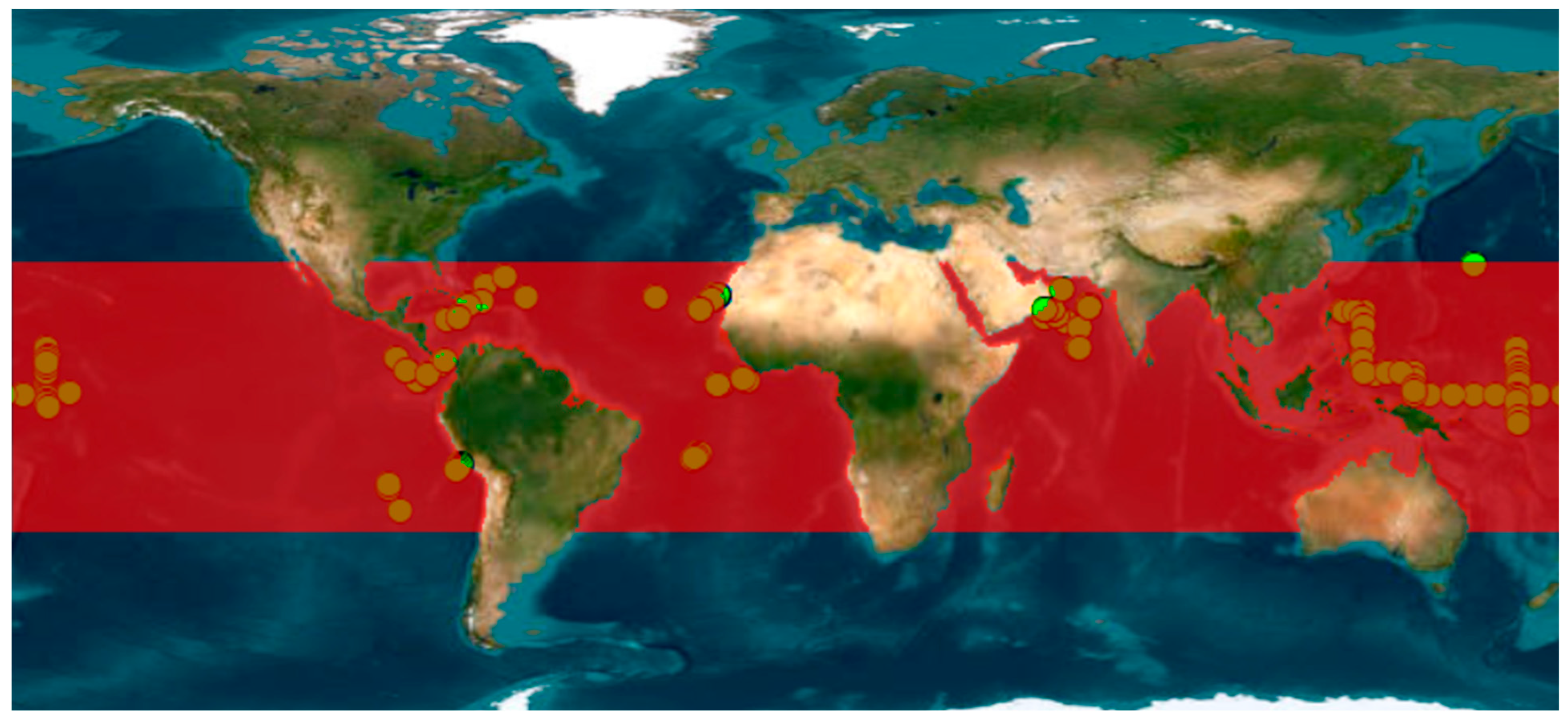
2.1. Input Data

The field ocean dataset used to investigate the relationship between sea temperature variations and ocean production included geographic coordinates, water temperature, Chl-a concentration and NPP estimates obtained using the 14C technique extracted from existing public repositories such as PANGEA and Ocean Productivity [23,24]. In this case, NPP is defined as the amount of carbon fixed by phytoplankton per unit time and sample volume and is a quantitative measure of primary production in aquatic environments [25,26,27,28].
Data from the tropical zone were specifically chosen for this analysis because this region is particularly vulnerable to the effects of water temperature variations [13]. In addition, studying this region allows for a clearer understanding of how Chl-a and NPP may interact with water temperature caused by the cyclical effects of El Niño occurring in the Pacific Ocean (Figure 1) [29,30].
Thus, for the tropical zone, the points monitored in the surface layers of the ocean were selected by web repositories and the filtering operation was applied to point data to exclude those with incomplete information. So, for each point the information includes the date of acquisition of the data, geographic information with latitude and longitude, day length, irradiance, sea temperature (expressed in °C), Chl-a concentration (expressed in mg m−3) and NPP concentration (expressed in mg m−3/day).
In addition, remote sensing imagery was selected from NASA’s Ocean Color sea surface temperature (SST) imagery derived from the Moderate Resolution Imaging Spectroradiometer, MODIS, a tool that collects remotely sensed data used by scientists to monitor, model and assess the impact of natural processes [31]. The images are available on the EARTHDATA platform and were acquired from January 2003 to December 2023 with monthly resolution and 9 km spatial resolution to build a time series of sea temperature useful for developing analytical workflows [32].

2.2. Performing Principal Component Analysis on a Dataset

In aquatic ecosystems research, it is essential to understand the key environmental factors that shape the dynamics of the system. Among these factors, temperature often plays a critical role, influencing physical, chemical and biological processes [16]. To determine whether temperature is the most important factor affecting the ecosystem, principal component analysis (PCA) was used to preserve the most important variability [33].
PCA was carried out using PAST software (Version 2.17) and allows us to identify and rank the variables that contribute most to the observed patterns within the ecosystem. By transforming the originally correlated variables into a set of uncorrelated principal components, PCA reveals the underlying structure of the data [34,35]. This approach is particularly valuable when dealing with complex environmental datasets where multiple factors interact. By applying PCA, we can simplify the interpretation of the data and prioritize the most influential variables [34,35].

2.3. Analysis Workflow Structure

The analytical workflow developed and tested in this study was built in R code on DataLabs virtual lab (https://datalabs.lifewatchitaly.eu/dashboard/ui/home accessed on 12 December 2024), a collaborative online coding platform provided by LifeWatch Italy, the Italian e-Science Infrastructure for biodiversity and ecosystem research. The DataLabs platform enables us to create and manage web services and analytical workflows using Python 3.10, R 4.3.0 and Matlab coding languages [36] and allowed the transformation of the code used in this study into web services, providing the advantage of more easily sharing the processes employed.
Mainly, the workflow reprocesses remote sensing imagery using a regression algorithm model derived from the ocean observing field dataset to analyze the variation in Chl-a and NPP in relation to sea surface temperature, with projections into the future.
The analytical workflow can be divided into three main steps. In the first step, a regression algorithm was developed using sea water temperature, Chl-a concentration and NPP data. In the second step, this algorithm was applied to sea surface temperature (SST) imagery for generating time series data for Chl-a and NPP. Finally, in the third step, the SST, Chl-a and NPP time series were projected into the future to forecast potential variations (Figure 2).

2.3.1. Step 1: Regression Model Definition

This step defines a good regression model to describe the pattern relation between Chl-a and NPP with water temperature. Field data of Chl-a, NPP and ocean temperature were used to train the linear regression and Random Forest algorithms to identify the better method that can describe the pattern of their relation. The cross-validation methodology was used to train and validate both models [37,38].
For each algorithm, the performance of the model was evaluated by calculating [37,39]:
  • R-squared (R2): Indicates the accuracy of the model, measuring the portion of the variance in observed data captured by the model. Its value ranges between 0 and 1. Values closer to 1 indicate a better performance of the data variance model, and vice versa, so values closer to 0 indicate a worse data variance model.
  • Mean Absolute Error (MAE): Indicates the accuracy of the model measuring the average absolute difference between observed and forecast value. Low values indicate good model performance.
  • Root Mean Squared Error (RMSE): Indicates the accuracy of the model by measuring the average of the squared difference between observed and forecast values. In this case, the accuracy is evaluated giving more importance to the larger errors. Low values indicate good model performance.
The R packages used to build the tool include the packages and functions caret, for training and tuning machine learning models, Random Forest, for implementing Random Forest regression, and lm, for applying linear regression models.

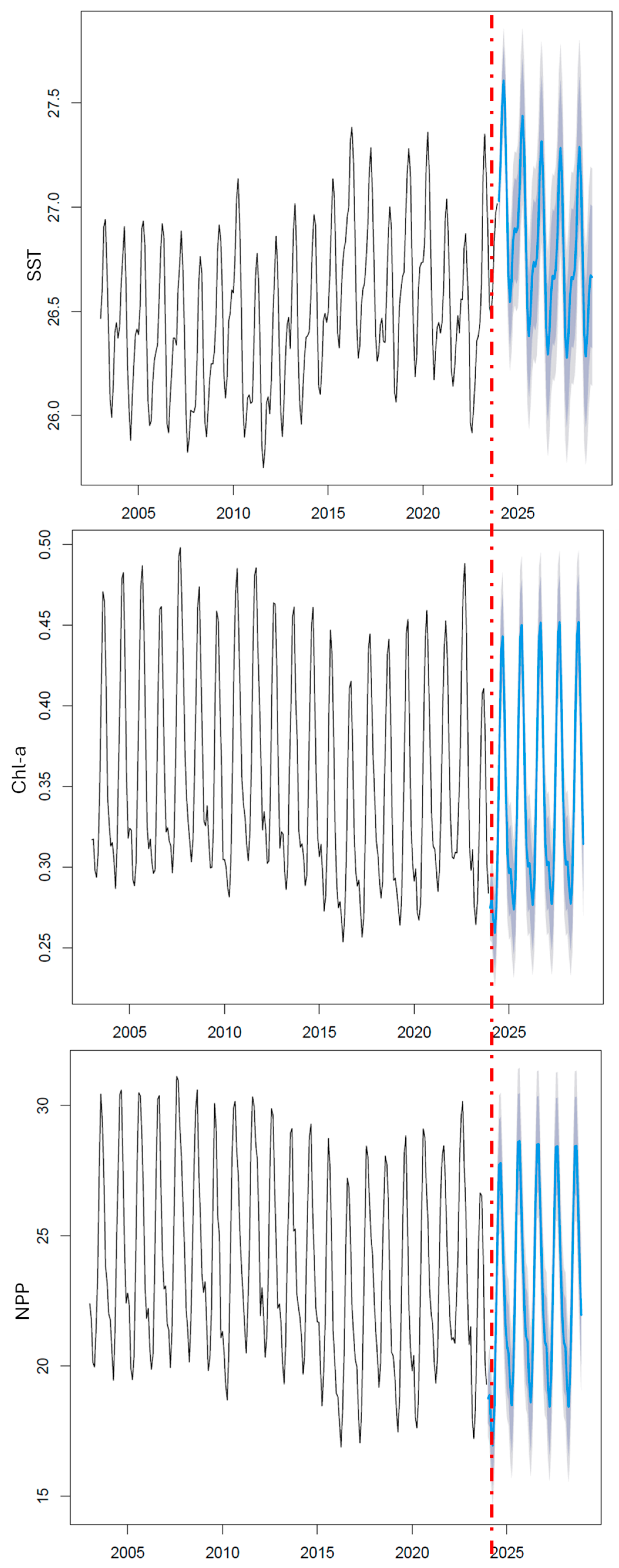
2.3.2. Step 2: SST, Chl-a and NPP Time Series Construction

In this step, SST, Chl-a and NPP time series were constructed for the study region. For the SST time series construction, based on the field data survey, the corresponding monthly MODIS SST images with a spatial resolution of 9 km were extracted using the shape file of the study area. Then, the mean SST value for the study area was calculated for each year considered. After that, Chl-a and NPP time series were calculated using the SST imagery. The better regression model derived from field ocean data in step 1 was applied to SST remote sensing imagery of the study area extrapolated from step 2 to produce a new dataset of Chl-a and NPP imagery products from 2003 to 2023. Then, the average value of Chl-a and NPP for each image was calculated to construct the time series and moving average was applied to highlight the trend. Kendall’s test was used to assess the statistical significance of the trend analysis in the relationship between time (which is progressive) and the values of the time series analyzed. The test returns Kendall’s tau value, which ranges from −1 (perfect decreasing trend) to 1 (perfect increasing trend) and the p-value. p-value < 0.05 indicates a statistically significant trend [40].
In ecology, time series of natural processes often exhibit distinct behavior, characterized by both periodic and irregular cycles. Studying these cyclical patterns of the ocean can provide valuable insights into the ecological resilience of the ecosystem services supported by phytoplankton by retrospectively assessing their ability to absorb significant past disturbances without compromising their essential ecological functions [18,19]. Therefore, to assess the short impact of SST perturbation events on Chl-a and NPP time series, recurrence analysis was employed. This advanced non-linear data analysis technique generates recurrence plots, which highlight the points in time when the dynamic system exhibits recurring behavior [12,38,41].
The R packages used to perform this step of analysis include dplyr for data manipulation and transformation; zoo and tseries for handling and analyzing time series data; sf for managing and analyzing geographic data; spdep for creating and managing spatial weight matrices; raster for managing and processing raster imagery and rgdal for handling vector data and performing spatial transformations.

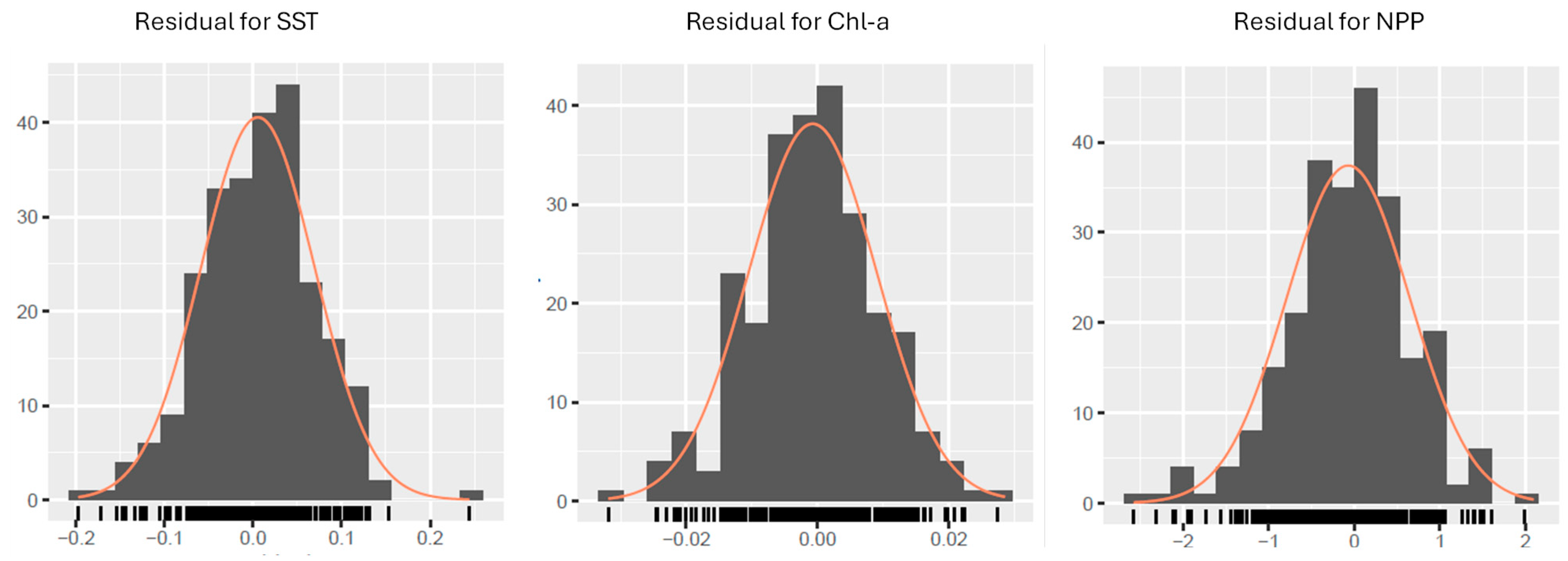
2.3.3. Step 3: Temporal Projection of the Time Series

To project the future evolution of SST, Chl-a and NPP time series from 2023 to the next five years, the Seasonal Autoregressive Integrated Moving Average (SARIMA) model, proposed by Box and Jenkins in 1970s [42], was applied. SARIMA is particularly suited for modeling and forecasting univariate time series data that exhibits a seasonal component, such as daily, monthly or annual patterns. By incorporating the seasonal component, SARIMA effectively captures recurring patterns in the data, making it a robust tool for projecting the trends in the time series analyzed.
The model for temporal projection of the time series consists of four main components [42,43,44]:
  • Seasonal (S): this component refers to the repeating patterns (daily, monthly, yearly or other) in the time series.
  • Autoregressive (AR): this component captures the relationship between the current data point and its previous values, accounting for the autocorrelation in the time series.
  • Integrated (I): this element transforms a non-stationary time series into a stationary one by applying differencing to reduce trends or seasonality.
  • Moving Average (MA): the MA component identifies short-term noise by analyzing the relationship between the current data point and past forecast errors.
The Box–Ljung test was used to analyze the residual autocorrelation derived by the SARIMA model, assessing the ability of the model to capture the underlying patterns in the time series data [45]. The test was applied across multiple lags, and a Bonferroni correction was used to mitigate the risk of false positives. Consequently, the significance level was adjusted by dividing the standard threshold of 0.05 by the number of tests performed (n = 20). As a result, a p-value below 0.0025 was considered significant, rather than the conventional 0.05.
Mean Absolute Error (MAE) and Root Mean Squared Error (RMSE) were calculated as performance metrics to assess the accuracy of the model [37,38]. The R package used to build the tool was Forecast.

3. Results

In this section, the results of each step of the analytical workflow are reported in three specific sections following the three steps of the workflow reported in Figure 2.

3.1. PCA

In the dataset analyzed, temperature emerges as the dominant factor in the first principal component, which captures the greatest variance, suggesting that temperature has a significant influence on the ecosystem’s behavior (Figure 3).
The confirmation of the role of temperature as a primary driver helps to guide the application of the machine learning model to study the direct responses of aquatic biomass, using Chl-a and NPP like a proxy, to temperature change.

3.2. Regression Model Definition

The linear and Random Forest models were trained and tested using five-fold cross-validation to predict Chl-a and NPP as a function of field-measured water temperature. The R-squared value showed the good ability of the applied regression models to capture part of the pattern of the observed data in both Chl-a and NPP variables. However, the Random Forest had a higher R-squared value than the linear model, indicating a better performance than the linear model in predicting Chl-a and NPP as a function of water temperature. In addition, the lower RMSE and MAE using Random Forest suggest that the quality of the predictions has improved in absolute terms compared with linear regression (Table 1).
Therefore, Random Forest was applied to the SST time series from MODIS imagery to predict the Chl-a and NPP time series.

3.3. Analytical Workflow

The mean SST of the study area exhibited a clear seasonal pattern, with consistent peaks observed in the moving average during four key periods such as 2009–2010, 2015–2016, 2019–2020 and 2023 (Figure 4).
From 2003 to 2009, the average SST displayed a decreasing trend. After this period, the SST trend reversed, showing a consistent increase, with a pronounced peak during 2015–2016 (Figure 4).
The trend analysis carried out with Kendall’s test applied to the SST time series highlighted a general upward trend from 2003 to 2023, with a positive tau value of 0.1838, which was statistically significant (p-value: 1.38 × 10⁻⁵). This indicates a general increase in SST over time.
The variation in SST had a negative impact on the temporal evolution of Chl-a and NPP because both time series exhibited a significant overall negative trend. Specifically, the Kendall test for the Chl-a time series resulted in a tau value of −0.1012 (p-value: 0.0168), while the NPP time series showed a tau value of −0.1143 (p-value: 0.0069). These results indicate a significant decline in Chl-a and NPP over time, led by the observed SST changes (Figure 4). The moving average revealed cyclical peaks in sea surface temperature (SST) from 2005 to 2012, and again from 2015 to 2023 (Figure 4). These peaks are likely to have been driven by the El Niño–Southern Oscillation (ENSO) phenomenon. ENSO is a climate phenomenon characterized by periodic fluctuations in SST across the central and eastern tropical Pacific. It includes both El Niño events, characterized by the anomalous warming of the surface waters, and La Niña events, associated with cooler-than-average SSTs [45].
The diagonal line in the recurrence plots, characterized by the succession of white dots in Figure 5, suggests that the system exhibits similar patterns of evolution over different time periods, indicating that the process may be deterministic [46]. However, the recurrence plot revealed that three of the peaks identified by the moving average window in the SST, Chl-a and NPP time series correspond to interruptions in the deterministic behavior of the system (Figure 5). These disruptions are likely caused by isolated perturbations that momentarily disrupt the system’s regular dynamic patterns at specific points in time. The disruptions shown in 2015–2017 and 2018–2020 can be linked to the alternance of the El Niño and La Niña events [29,30], whereas the peak in 2023 could correspond to La Niña. Therefore, only the ENSO events shown in box 1 of Figure 4 highlight any relevant impacts on SST dynamics, with relative alterations to Chl-a and NPP dynamics (Figure 5). Thus, in this analysis of the time series patterns it is possible to highlight both the influence of the SST trend on the biotic variable and the decreasing peaks potentially generated by ENSO events (Figure 4 and Figure 5).

3.4. Projection of the Time Series into the Future

The SARIMA model was applied to the three time series to forecast the evolution of SST, Chl-a and NPP over the next five years (Figure 4). The model predicts an increase in SST in 2024, followed by a decline in subsequent years, while Chl-a and NPP are expected to decrease in 2024, with a slight increase in the following years. Nonetheless, SST levels during the later period (2014 to 2025) are projected to remain higher than those in the early years (2003). In contrast, the levels of the biotic components, Chl-a and NPP, are forecasted to remain below their initial values recorded in 2003 (Figure 6). The MAE and RMSE showed a low value, which may indicate the good accuracy of the model in predicting the values of SST, Chl-a and NPP in relation to the real values (Table 2).
The residuals from the model exhibited homoscedasticity, as they followed a normal distribution with the values centered around zero (Figure 7).
The Box–Ljung test showed that, at different lags, the residuals for SST and Chl-a consistently showed no significant autocorrelation. This suggests that the SARIMA model adequately fits the data patterns (Table 3). In contrast, the residuals for NPP exhibited significant autocorrelation, indicating that the model does not adequately capture the underlying pattern in this case. Thus, on the basis of the time series analyzed, the SARIMA forecasting model allows the development of a short-term forecast for Chl-a, while it does not produce a significant forecasting result for NPP.

4. Discussion

The analytical workflow used a machine learning algorithm to develop a preliminary model based on field measurements of the abiotic and biotic parameters of aquatic biomass.
While it is well documented that non-linear models, such as Random Forest, generally outperform linear models, the effectiveness of machine learning analysis is strongly influenced by the specific characteristics of the data. Thus, we included and applied both linear regression and non-linear models in the analytical workflow in order to (i) test which model fits better to the data analyzed, (ii) improve the flexibility of the overall analytical workflow on DataLabs, which can be reused by multiple users according to their data needs. Therefore, the integration of the linear model, although the Random Forests algorithm is better than linear fitting, could be useful for future applications in different case studies and with different datasets.
In this case study, Random Forest was robust to noise and outliers, and more effective in dealing with such anomalies and non-linear information. Linear regression, on the other hand, is more sensitive to outliers, which can distort the fit of the model [46,47]. In summary, Random Forests were better suited to this type of data because they can capture non-linear relationships, interaction effects and threshold behaviors in the relationship between sea temperature, Chl-a and NPP. In contrast, linear regression, which assumes a simpler, linear relationship, was less appropriate to reflect the complexity of environmental systems. As our results confirmed previous findings on the effectiveness of the Random Forest algorithm over the linear model, this suggests that the relationships between sea temperature, chlorophyll-a (Chl-a) and net primary production (NPP) are likely to be characterized by non-linear behaviors. This may mean that the relationships between sea temperature, Chl-a and NPP are likely to be characterized by non-linear behaviors. In addition, other environmental factors, such as nutrient concentrations, may indirectly influence this relationship, contributing to more complex patterns that Random Forest is better able to capture than linear regression [47,48].
The Random Forest model, analyzing the relationship between sea temperature, Chl-a and NPP, applied to MODIS SST time series proved to be a valuable tool for detecting spatial and temporal variations in response to climate change. By integrating field surface measurements with SST data from MODIS imagery, the model significantly enhanced the predictive capability for Chl-a and SST variations. In the tropical zone, SST data reveal a general upward trend. This upward trend in SST is associated with a corresponding decrease in Chl-a and NPP. Additionally, the SST time series highlighted four prominent peaks, which corresponded to four lower peaks in Chl-a and NPP.
Two types of dynamics have been observed from the SST, Chl-a and NPP trends:
  • Long-term dynamics from 2003 to 2023, which may be driven by global warming, which poses a greater risk to the system, potentially leading to significant long-term disruptions if the trend continues.
  • Short-term dynamics, which may be result from cycle perturbation events, such as ENSO events, which introduce temporary disruptions represented by the non-stationary evolution of the system, which is far from the current evolution of the system in the analyzed time frame [49,50].
Overall, while the long-term trend driven by global warming could have severe implications for the ecosystem, the system’s ability to recover from ENSO-related disturbances actually suggests a level of resilience to short-term variations. Resilience in this case is interpreted as the ability of the system to recover the behavior pattern data after the perturbation event [41]. This consideration, however, is contextualized by the length of the 21-year analysis time series determined by the availability of MODIS images. Moreover, the analytical workflow was tested using the SST time series with a monthly time step. This may have limited the system’s ability to distinguish the impact of ENSO on variations in its recurrence behavior, for example, between 2005 and 2012. In future, incorporating imagery with higher temporal resolution and time frequency could enhance this analysis.
The combined effects of global warming and ENSO events have resulted in an increase in the sea surface temperature of 0.030 °C per year, which may have contributed to a decrease in the Chl-a concentration of 0.003 units per year and a decrease in the rate of NPP of 0.160 units per year. These values should not be interpreted as precise quantitative measurements, but rather as qualitative indicators of the rate of change in the abiotic factors affecting aquatic biomass. The time series data reflect discrete rather than continuous changes in these variables over time.
The depletion of Chl-a and NPP highlighted here can have negative impacts on the provision of ecosystem services associated with the absorption of CO2, which is important for climate regulation. In addition, the temporal reduction in Chl-a can negatively impact the provision of services such as food production. This can have social implications in the context of food security linked to the tropical zone, which represents the capacity of the system to guarantee food security like the quantity and quality of food production [51], with consequent negative impacts on the local economy [50,52]. A more direct ecological implication of these results could be that the mismatch between increasing temperatures and declining levels of Chl-a and NPP suggests that primary productivity might not be keeping pace with the heightened metabolic requirements of animals at higher trophic levels induced by rising temperatures [53,54]. This imbalance could have far-reaching consequences for the mechanisms of coexistence and species interactions [55].
Forecasting analysis suggests that the increase in sea surface temperature (SST) should begin to slow after 2024, when the current ENSO event is expected to end. This could lead to a stabilization of Chl-a, though it is likely to remain at lower levels compared with past averages. Unfortunately, the prediction of NPP was not reliable because the residual showed high autocorrelation at different lags, so it is necessary to re-run the model with new data, apply variable transformation or change the model parameters. However, this is not currently part of the analytical workflow as it requires the manual manipulation of the data and a different specific approach. However, this is only one way of exploring the potential applications of field data with remote sensing data using machine learning. Another perspective could be to use the available field data in combination with MODIS Chl-a and SST images or another remote sensing sensor to generate a new estimate of NPP. Currently, a limitation of this study is the relatively small number of field measurement points in the dataset used, which may reduce the overall representativeness of the system being studied.
Overall, although there are a few limitations mainly linked to the relatively small number of field measurement points in the dataset used, the analytical workflow developed and tested in this study could be seen as a preliminary attempt to understanding ecosystem services responses to ocean temperature variation. Thus, the analytical workflow has the potential to track climate-driven changes in oceanic ecosystems, especially in regions sensitive to such large-scale climate processes and can be refined over time by incorporating additional datasets to enhance its accuracy and applicability.

5. Conclusions

The analytical workflow developed in this study provides a robust and reproducible initial approach for analyzing the impact of climate change on phytoplankton ecological processes in aquatic ecosystems. This could have significant implications for the sustainable management of aquatic ecosystems and their ability to provide ecosystem services.
The proposed approach proved particularly effective in managing complex environmental datasets with multiple interacting variables. Identifying sea surface temperature (SST) as the system’s key driver simplified the interpretation of data and enabled modeling efforts to focus on the most influential climatic variable. In this context, the workflow can serve as a valuable tool for supporting non-ICT experts in monitoring and predicting changes in aquatic biomass in relation to SST dynamics.
The results emphasize the importance of integrating local and global datasets within a unified analytical system. Combining remote sensing data and in situ measurements, and processing them through machine learning algorithms, significantly enhanced the system’s predictive capability. This offered improved temporal insights into ongoing, climate-driven transformations.
Future development of the workflow may involve estimating net primary production (NPP) by directly combining sea surface temperature (SST) and chlorophyll-a (Chl-a) data from MODIS or other satellite sensors. This approach would address the limitations posed by the scarcity of field observations and improve the system’s predictive performance.
Moreover, to improve the flexibility of the analytical workflow in response to different needs and enhance the accuracy of its analysis, remote sensing imagery with a higher spatial and temporal resolution could be incorporated. This would allow for better discrimination of the cyclicality in the time series and improve the analysis. This goal could also be achieved by using products similar to MODIS products, such as SST, but with a higher spatial and temporal resolution.
That being said, while there are opportunities for improvement, it is important to highlight that the workflow also stands out for its versatility. It can easily be adapted to different geographical and environmental contexts, such as continental coastal zones or oligotrophic marine regions, simply by uploading different field datasets and defining a new study area. Furthermore, its implementation on the Datalabs platform ensures the workflow is reproducible, accessible and interoperable in line with the FAIR principles. This also makes it a valuable tool for researchers without specific expertise in remote sensing.

Author Contributions

Conceptualization, T.S.; methodology, T.S.; software, T.S.; validation, T.S., J.T., L.L. and F.M.; formal analysis, T.S.; investigation, T.S., J.T., L.L. and F.M.; resources, T.S., J.T., L.L. and F.M.; data curation, T.S., J.T., L.L. and F.M.; writing—original draft preparation, T.S.; writing—review and editing, T.S., J.T., L.L., F.M., F.D.L., G.I., M.S. and A.B.; visualization, T.S., J.T., L.L., F.M., G.I., F.D.L., M.S. and A.B.; supervision, A.B.; project administration, A.B.; funding acquisition, A.B. All authors have read and agreed to the published version of the manuscript.

Funding

The publication has been funded by EU—Next Generation EU Mission 4 “Education and Research”—Component 2: “From research to business”—Investment 3.1: “Fund for the realization of an integrated system of research and innovation infrastructures”—Project IR0000032—ITINERIS—Italian Integrated Environmental Research Infrastructures System—CUP B53C22002150006.

Data Availability Statement

The raw data supporting the conclusions of this article will be made available by the authors on request.

Acknowledgments

The authors acknowledge the Research Infrastructures participating in the ITINERIS project with their Italian nodes: ACTRIS, ANAEE, ATLaS, CeTRA, DANUBIUS, DISSCO, e-LTER, ECORD, EMPHASIS, EMSO, EUFAR, Euro-Argo, EuroFleets, Geoscience, IBISBA, ICOS, JERICO, LIFEWATCH, LNS, N/R Laura Bassi, SIOS and SMINO.

Conflicts of Interest

The authors declare no conflicts of interest. Views and opinions expressed are, however, those of the authors only and do not necessarily reflect those of the European Union or the European Commission. Neither the European Union nor European Commission can be held responsible for them.

Abbreviations

The following abbreviations are used in this manuscript:
Chl-aChlorophyll-a
NPPNet Primary Production
SSTSea Surface Temperature
ENSOEl Niño–Southern Oscillation

References

  1. Garrison, T.S. Oceanography: An Invitation to Marine Science; Thompson Brooks/Cole: Baltimore, MD, USA, 2005; Volume 4. [Google Scholar]
  2. Barbier, E.B. Marine ecosystem services. Curr. Biol. 2017, 27, R507–R510. [Google Scholar] [CrossRef] [PubMed]
  3. Costanza, R.; Fisher, B.; Mulder, K.; Liu, S.; Christopher, T. Biodiversity and ecosystem services: A multi-scale empirical study of the relationship between species richness and net primary production. Ecol. Econ. 2007, 61, 478–491. [Google Scholar] [CrossRef]
  4. Wirtz, K.; Smith, S.L.; Mathis, M.; Taucher, J. Vertically migrating phytoplankton fuel high oceanic primary production. Nat. Clim. Change 2022, 12, 750–756. [Google Scholar] [CrossRef]
  5. World Ocean Review. WOR 8 The Ocean—A Climate Champion? How to Boost Marine Carbon Dioxide Uptake. 2024. Available online: https://worldoceanreview.com/en/wor-8/the-role-of-the-ocean-in-the-global-carbon-cyclee/how-the-ocean-absorbs-carbon-dioxide/ (accessed on 10 January 2025).
  6. Canadell, J.G.; Monteiro, P.M.S.; Costa, M.H.; da Cunha, L.C.; Cox, P.M.; Eliseev, A.V.; Henson, S.; Ishii, M.; Jaccard, S.; Koven, C.; et al. Global Carbon and other Biogeochemical Cycles and Feedbacks. In Climate Change 2021: The Physical Science Basis; Contribution of Working Group I to the Sixth Assessment Report of the Intergovernmental Panel on Climate Change; Masson-Delmotte, V., Zhai, P., Pirani, A., Connors, S.L., Péan, C., Berger, S., Caud, N., Chen, Y., Goldfarb, L., Gomis, M.I., et al., Eds.; Cambridge University Press: Cambridge, UK; New York, NY, USA, 2021; pp. 673–816. [Google Scholar] [CrossRef]
  7. Mapping Ocean Wealth. Esosystem Services. Available online: https://oceanwealth.org/ecosystem-services/ (accessed on 23 February 2025).
  8. Vuong, Q.-H.; Duong, M.-P.T.; Nguyen, Q.-Y.T.; La, V.-P.; Nguyen, P.-T.; Nguyen, M.-H. Ocean economic and cultural benefit perceptions as stakeholders’ constraints for supporting conservation policies: A multi-national investigation. Mar. Policy 2024, 163, 106134. [Google Scholar] [CrossRef]
  9. Le Quéré, C.; Moriarty, R.; Andrew, R.M.; Peters, G.P.; Ciais, P.; Friedlingstein, P.; Jones, S.D.; Sitch, S.; Tans, P.; Arneth, A.; et al. Global carbon budget 2014. Earth Syst. Sci. Data 2015, 7, 47–85. [Google Scholar] [CrossRef]
  10. Costello, C.; Cao, L.; Gelcich, S.; Cisneros-Mata, M.Á.; Free, C.M.; Froehlich, H.E.; Golden, C.D.; Ishimura, G.; Maier, J.; Macadam-Somer, I.; et al. The future of food from the sea. Nature 2020, 588, 95–100. [Google Scholar] [CrossRef]
  11. Lungomela, C.; Nyamisi, P. Chapter 10: Phytoplankton and Ocean Primary Productivity. In State of the Coast, for mainland Tazania; Transitioning to Blue Economy: Contribution of Coastal and marine Environmental; Mangora, M.M., Msangameno, D.J., Woiso, J.F., Eds.; Western Indian Ocean Marine Science Association (WIOMSA): Zanzibar, Tanzania, 2024; ISBN 978-9912-9882-0-0. [Google Scholar]
  12. A Climate Change Dashboard. Available online: https://chpdb.it/_climate_dash/index.php?tag=temperatura (accessed on 15 July 2024).
  13. Woodhouse, A.; Swain, A.; Fagan, W.F.; Fraass, A.J.; Lowery, C.M. Late Cenozoic cooling restructured global marine plankton communities. Nature 2023, 614, 713–718. [Google Scholar] [CrossRef] [PubMed]
  14. Racault, M.-F.; Sathyendranath, S.; Brewin, R.J.W.; Raitsos, D.E.; Jackson, T.; Platt, T. Impact of El Niño Variability on Oceanic Phytoplankton. Front. Mar. Sci. 2017, 4, 133. [Google Scholar] [CrossRef]
  15. Arteaga, L.A.; Rousseaux, C.S. Impact of Pacific Ocean heatwaves on phytoplankton community composition. Commun. Biol. 2023, 6, 263. [Google Scholar] [CrossRef]
  16. Sigman, D.M.; Hain, M.P. The Biological Productivity of the Ocean. Nat. Educ. Knowl. 2012, 3, 21. [Google Scholar]
  17. Cervantes-Duarte, R.; González-Rodríguez, E.; Funes-Rodríguez, R.; Ramos-Rodríguez, A.; Torres-Hernández, M.Y.; Aguirre-Bahena, F. Variability of Net Primary Productivity and Associated Biophysical Drivers in Bahía de La Paz (Mexico). Remote Sens. 2021, 13, 1644. [Google Scholar] [CrossRef]
  18. Semeraro, T.; Luvisi, A.; Lillo, A.; Aretano, R.; Buccolieri, R.; Marwan, N. Recurrence Analysis of Vegetation Indices for Highlighting the Ecosystem Response to Drought Events: An Application to the Amazon Forest. Remote Sens. 2020, 12, 907. [Google Scholar] [CrossRef]
  19. Semeraro, T.; Buccolieri, R.; Vergine, M.; De Bellis, L.; Luvisi, A.; Emmanuel, R.; Marwan, N. Analysis of Olive Grove Destruction by Xylella fastidiosa Bacterium on the Land Surface Temperature in Salento Detected Using Satellite Images. Forests 2021, 12, 1266. [Google Scholar] [CrossRef]
  20. Barbosa, C.C.A.; Atkinson, P.M.; Dearing, J.A. Remote sensing of ecosystem services: A systematic review. Ecol. Indic. 2015, 52, 430–443. [Google Scholar] [CrossRef]
  21. Amani, M.; Moghimi, A.; Mirmazloumi, S.M.; Ranjgar, B.; Ghorbanian, A.; Ojaghi, S.; Ebrahimy, H.; Naboureh, A.; Nazari, M.E.; Mahdavi, S.; et al. Ocean Remote Sensing Techniques and Applications: A Review (Part I). Water 2022, 14, 3400. [Google Scholar] [CrossRef]
  22. Cao, Z.; Ma, R.; Duan, H.; Pahlevan, N.; Melack, J.; Shen, M.; Xue, K. A machine learning approach to estimate chlorophyll-a from Landsat-8 measurements in inland lakes. Remote Sens. Environ. 2020, 248, 111974. [Google Scholar] [CrossRef]
  23. Ocean Productivity. Available online: http://orca.science.oregonstate.edu/npp_products.php (accessed on 10 June 2024).
  24. PANGAEA. Data Publisher for Earth & Environmental Science. Available online: https://www.pangaea.de/ (accessed on 10 January 2025).
  25. Redalje, D.G.; Laws, E.A. A new method for estimating phytoplankton growth rates and carbon biomass. Mar. Biol. 1981, 62, 73–79. [Google Scholar] [CrossRef]
  26. Hein, M.; Riemann, B. Nutrient limitation of phytoplankton biomass or growth rate: An experimental approach using marine enclosures. J. Exp. Mar. Biol. Ecol. 1995, 188, 67–180. [Google Scholar] [CrossRef]
  27. Steeman Nielsen, E.; Jensen, E.A. The autotrophic production of organic matter in the oceans. Calathea Rep. 1957, 1, 49–124. [Google Scholar]
  28. Marra, J. Net and gross productivity: Weighting in with 14C. Aquat. Microb. Ecol. 2009, 56, 123–131. [Google Scholar] [CrossRef]
  29. Siswanto, E.; Ye, H.; Yamazaki, D.; Tang, D. Detailed spatiotemporal impacts of El Niño on phytoplankton biomass in the South China Sea. J. Geophys. Res. Ocean. 2017, 12, 2709–2723. [Google Scholar] [CrossRef]
  30. World Health Organization. El Niño Southern Oscillation (ENSO). 2024. Available online: https://www.who.int/news-room/fact-sheets/detail/el-nino-southern-oscillation-(enso) (accessed on 8 September 2024).
  31. Christopher, J. Internal wave detection using the Moderate Resolution Imaging Spectroradiometer (MODIS). J. Geophys. Res. 2007, 112, C11012. [Google Scholar] [CrossRef]
  32. EARTHDATA. Ocean Color. Available online: https://oceancolor.gsfc.nasa.gov/ (accessed on 1 December 2024).
  33. Peres-Neto, P.R.; Jackson, D.A.; Somers, K.M. Giving meaningful interpretation to ordination axes: Assessing loading significance in principal component analysis. Ecology 2003, 84, 2347–2363. [Google Scholar] [CrossRef]
  34. Elhaik, E. Principal Component Analyses (PCA)-based findings in population genetic studies are highly biased and must be reevaluated. Sci. Rep. 2022, 12, 14683. [Google Scholar] [CrossRef]
  35. Ilin, A.; Raiko, T. Practical approaches to Principal Component Analysis in the presence of missing values. J. Mach. Learn. Res. 2010, 11, 1957–2000. [Google Scholar]
  36. LifeWatchItaly. DataLabs: LifeWatch’s Collaborative Coding Platform for Biodiversity and Ecosystem Research. Available online: https://datalabs.lifewatchitaly.eu/ (accessed on 15 July 2024).
  37. Rodriguez-Galiano, V.; Sanchez-Castillo, M.; Chica-Olmo, M.; Chica-Rivas, M. Machine learning predictive models for mineral prospectivity: An evaluation of neural networks, random forest, regression trees and support vector machines. Ore Geol. Rev. 2015, 71, 804–818. [Google Scholar] [CrossRef]
  38. Ramezan, C.A.; Warner, T.A.; Maxwell, A.E. Evaluation of Sampling and Cross-Validation Tuning Strategies for Regional-Scale Machine Learning Classification. Remote Sens. 2019, 11, 185. [Google Scholar] [CrossRef]
  39. Hu, S.; Liu, H.; Zhao, W.; Shi, T.; Hu, Z.; Li, Q.; Wu, G. Comparison of Machine Learning Techniques in Inferring Phytoplankton Size Classes. Remote Sens. 2018, 10, 191. [Google Scholar] [CrossRef]
  40. Kendall, M.G. Rank Correlation Methods, 4th ed.; Charles Griffin: London, UK, 1975. [Google Scholar]
  41. Marwan, N.; Carmen Romano, M.; Thiel, M.; Kurths, J. Recurrence plots for the analysis of complex systems. Phys. Rep. 2007, 438, 237–329. [Google Scholar] [CrossRef]
  42. Mao, Q.; Zhang, K.; Yan, W.; Cheng, C. Forecasting the incidence of tuberculosis in China using the seasonal auto-regressive integrated moving average (SARIMA) model. J. Infect. Public Health 2018, 11, 707–712. [Google Scholar] [CrossRef]
  43. Adams, S.O.; Mustapha, B.; Alumbugu, A.I. Seasonal Autoregressive Integrated Moving Average (SARIMA) Model for the Analysis of Frequency of Monthly Rainfall in Osun State, Nigeria. Phys. Sci. Int. J. 2019, 22, 1–9. Available online: https://ssrn.com/abstract=4338971 (accessed on 10 August 2019). [CrossRef]
  44. Zhang, X.; Pang, Y.; Cui, M.; Stallones, L.; Xiang, H. Forecasting mortality of road traffic injuries in China using seasonal autoregressive integrated moving average model. Ann. Epidemiol. 2015, 25, 101–106. [Google Scholar] [CrossRef] [PubMed]
  45. The NOAA Physical Sciences Laboratory. Available online: https://psl.noaa.gov/about/ (accessed on 25 January 2025).
  46. Hassani, H.; Yeganegi, M.R. Selecting optimal lag order in Ljung–Box test. Phys. A Stat. Mech. Its Appl. 2020, 541, 123700. [Google Scholar] [CrossRef]
  47. Smith, P.F.; Ganesh, S.; Liu, P. A comparison of random forest regression and multiple linear regression for prediction in neuroscience. J. Neurosci. Methods 2013, 220, 85–91. [Google Scholar] [CrossRef]
  48. Xie, X.; Wu, T.; Zhu, M.; Jiang, G.; Xu, Y.; Wang, X.; Pu, L. Comparison of random forest and multiple linear regression models for estimation of soil extracellular enzyme activities in agricultural reclaimed coastal saline land. Ecol. Indic. 2021, 120, 106925. [Google Scholar] [CrossRef]
  49. Wang, C.; Fiedler, P.C. ENSO variability and the eastern tropical Pacific: A review. Prog. Oceanogr. 2006, 69, 239–266. [Google Scholar] [CrossRef]
  50. Liu, Y.; Cai, W.; Lin, X.; Li, Z.; Zhang, Y. Nonlinear El Niño impacts on the global economy under climate change. Nat. Commun. 2022, 14, 5887. [Google Scholar] [CrossRef]
  51. Semeraro, T.; Scarano, A.; Curci, L.M.; Leggieri, A.; Lenucci, M.; Basset, A.; Santino, A.; Piro, G.; De Caroli, M. Shading effects in agrivoltaic systems can make the difference in boosting food security in climate change. Appl. Energy 2024, 358, 122565. [Google Scholar] [CrossRef]
  52. Barber, R.T.; Chavez, F.P. Biological Consequences of El Niño. Science 1983, 222, 1203–1210. [Google Scholar] [CrossRef]
  53. Shokri, M.; Cozzoli, F.; Vignes, F.; Bertoli, M.; Pizzul, E.; Basset, A. Metabolic rate and climate change across latitudes: Evidence of mass-dependent responses in aquatic amphipods. J. Exp. Biol. 2022, 225, jeb244842. [Google Scholar] [CrossRef]
  54. Shokri, M.; Lezzi, L.; Basset, A. The seasonal response of metabolic rate to projected climate change scenarios in aquatic amphipods. J. Therm. Biol. 2024, 124, 103941. [Google Scholar] [CrossRef] [PubMed]
  55. Shokri, M.; Cozzoli, F.; Basset, A. Metabolic rate and foraging behaviour: A mechanistic link across body size and temperature gradients. Oikos 2025, 2025, e10817. [Google Scholar] [CrossRef]
Figure 1. The study area and the sampling points to be considered for the study. The dots represent the sampling sites, while the red band represents the study area.
Environments 12 00210 g001
Figure 2. The diagram represents the workflow analysis developed for case study.
Environments 12 00210 g002
Figure 3. Key variables and their contribution from principal component analysis.
Environments 12 00210 g003
Figure 4. Time series of SST (A), Chl-a (B) and NPP (C). The moving average is shown in red. The sky-blue boxes represent the temperature peaks where temperature perturbations, such as ENSO events, occur. Boxes 1 and 2 show the time window during which peaks in the time series were observed.
Environments 12 00210 g004
Figure 5. Recurrence plot of SST (A), Chl-a (B) and NPP (C) time series. White lines are represented by a series of dots. Each white dot represents one of the recurrence points of the system. The yellow boxes represent the part of the Recurrence Plots where there are perturbations in the systems due to perturbation events such as ENSO.
Environments 12 00210 g005
Figure 6. The results of the SARIMA prediction model applied to the SST, Chl-a and NPP time series, where the red line represents the start of new scenarios. The blue line after 2023 represents the estimated value, while the gray line represents the maximum and minimum confidence intervals.
Environments 12 00210 g006
Figure 7. Distribution of the residuals for the SST, Chl-a and NPP time series analyzed with the SARIMA model.
Environments 12 00210 g007
Table 1. Accuracy analysis of the regression models applied to the sample dataset.
ModelBiotic ParametersR2MAERMSE
Linear regressionChl-a0.60193730.77510630.9543401
NPP0.40810171.0474331.240625
Random ForestChl-a0.7526840.56697730.7623114
NPP0.61120260.7548110.9819766
Table 2. Accuracy analysis of the SARIMA forecast model applied to the SST, Chl-a and NPP variables (SST expressed in °C, Chl-a expressed in mg m−3 and NPP expressed in mg m−3/day).
VariableMAERMSE
SST0.050895510.0644293
Chl-a0.0075729480.009766999
NPP0.72263670.5497908
Table 3. Box–Ljung test applied to different lags to assess the autocorrelation of the residuals of the SST, Chl-a and NPP time series.
LagSST p-ValueChl-a p-ValueNPP p-Value
60.049850.20260.071
120.16040.15010.07359
240.54310.20270.01291
360.66840.29580.006218
480.82420.42980.01163
600.94210.35630.005601
720.85310.2130.006164
840.76140.15740.004539
960.85540.18950.003743
1080.8250.11510.001579
1200.86830.22140.003643
1320.83520.040860.0001627
1480.86270.057030.0001433
1500.88630.060340.0001357
1620.87910.055930.0001735
1740.930.076110.0004293
1860.93170.07020.000794
1980.96750.07460.001189
2100.87960.11720.003056
2220.81910.23120.005376
2340.7970.2420.005095
Disclaimer/Publisher’s Note: The statements, opinions and data contained in all publications are solely those of the individual author(s) and contributor(s) and not of MDPI and/or the editor(s). MDPI and/or the editor(s) disclaim responsibility for any injury to people or property resulting from any ideas, methods, instructions or products referred to in the content.

