Article

Street-Level Sensing for Assessing Urban Microclimate (UMC) and Urban Heat Island (UHI) Effects on Air Quality

by
Lirane Kertesse Mandjoupa
1,*,†,
Pradeep Behera
1,
Kibria K. Roman
2,
Hossain Azam
1 and
Max Denis
1,†
1
Department of Civil and Mechanical Engineering, School of Engineering and Applied Sciences, University of the District of Columbia, 4200 Connecticut Avenue NW, Washington, DC 20008, USA
2
Department of Mechanical Engineering and ARES, State University of New York Canton, Canton, NY 13617, USA
*
Author to whom correspondence should be addressed.
These authors contributed equally to this work.
Environments 2025, 12(6), 184; https://doi.org/10.3390/environments12060184
Submission received: 18 February 2025 / Revised: 17 May 2025 / Accepted: 18 May 2025 / Published: 30 May 2025

Abstract

During the intense heatwaves of late summer 2024, Washington, D.C.’s urban landscape revealed the powerful influence of urban morphology on microclimates and air quality. This study investigates the impact of building height-to-width (H/W) ratios on the urban heat island (UHI) effect, using a combination of field measurements and Computational Fluid Dynamics (CFD) simulations to understand the dynamics. Street-level data collected from late August to November 2024 across three sites in Washington, D.C., indicate that high H/W ratios (1.5–2.0) increased temperatures by approximately 2–3 °C and reduced wind speeds to around 0.8 m/s. These conditions led to elevated pollutant concentrations, with ozone (O3) ranging from 1.8 to 7.3 ppb, nitrogen dioxide (NO2) from 0.3 to 0.5 ppm, and carbon monoxide (CO) remaining relatively constant at approximately 2.1 ppm. PM2.5 concentrations fluctuated between 2.8 and 0.4 μ g/m3. Meanwhile, lower H/W ratios (less than 1.5) demonstrated better air circulation and lower pollution levels. The CFD simulations are in agreement with the experimental data, yielding an RMSE of 0.75 for temperature, demonstrating its utility for forecasting UHI effects under varying urban layouts. These results demonstrate the potential of Computational Fluid Dynamics in not only modeling but also predicting UHI dynamics.

1. Introduction

The Urban Heat Island (UHI) phenomenon occurs when urban areas exhibit higher temperatures than their rural surroundings, with temperature differences ranging from 1 °C to 7 °C [1,2]. This phenomenon arises from a combination of factors, including the absorption and retention of heat by urban infrastructure, anthropogenic heat release, and reduced vegetative cover [3,4].
Urban microclimates, shaped by localized climatic conditions, exacerbate UHI effects such as heat retention, reduced nighttime cooling, and pollutant buildup in street canyons [5]. Furthermore, the interaction between UHI and air quality has significant health implications. The elevated temperatures caused by UHI accelerate chemical reactions in the atmosphere, leading to increased concentrations of pollutants such as tropospheric ozone and fine particulate matter. These pollutants contribute to respiratory diseases, cardiovascular diseases, and heat stress, particularly in vulnerable populations [6,7]. In addition, urban areas with high-density traffic and industrial activity experience compounded effects, where heat and pollution form a feedback loop that intensifies both phenomena.
To study the complexity of the interaction between Urban Heat Island (UHI) and urban microclimates, researchers have adopted diverse measurement methods, each with unique advantages and limitations. Traditional meteorological stations, such as those of Santamouris to analyze urban heat islands in Europe, provide long-term reliable data but often lack the spatial resolution needed to capture detailed urban variability effectively [8]. Similarly, Yang et al. used network of weather stations to explore urban microclimates, highlighting their utility but also their limitations in representing spatial heterogeneity [9]. Remote sensing techniques, particularly satellite-based Land Surface Temperature (LST) data, offer valuable large-scale insights. For example, the Moderate Resolution Imaging Spectroradiometer (MODIS) and Landsat have been extensively used to monitor urban microclimates due to their high spatial resolution [10,11]. However, these methods require complementary in situ data to validate findings and address low temporal resolution [11]. Mobile monitoring sensing tools, including wearable devices and vehicle-based platforms, provide a finer spatial understanding of microclimatic variations.
Computational Fluid Dynamics (CFD) models, particularly Reynolds-Averaged Navier-Stokes (RANS) models, play a crucial role in simulating urban airflow, pollutant dispersion, and temperature patterns. Recent advancements, such as those by Kavian et al. [12], have improved the accuracy of RANS models for urban pollutant flow simulations by optimizing empirical coefficients using genetic algorithms. These enhancements have led to more accurate predictions of pollutant dispersion within clusters of urban buildings. Additionally, CFD simulations utilizing RANS models have been instrumental in analyzing wind flow and pollutant distribution in street canyons affected by vehicular traffic.
Li et al. [13] compared RANS with Large Eddy Simulation (LES) models and concluded that RANS, particularly the standard k- ε turbulence model, offered reliable predictions for mean wind velocity and pollutant concentrations in urban environments. In recent years, CFD simulations of urban microclimates have predominantly employed the commercial tool ANSYS Fluent 2025 R1, followed by OpenFOAM and ENVI-met. Together, these three platforms account for over 90% of all urban CFD simulations. ENVI-met (Windows-based) and OpenFOAM (Linux/Ubuntu-based) are especially popular for simulating urban canopy models, owing to their ability to handle complex three-dimensional urban geometries and their inclusion of specialized solver packages.
ENVI-met, a piece of three-dimensional computational fluid dynamics (CFD) software, has emerged as a widely used tool for analyzing urban microclimates and their interactions with environmental parameters. Its ability to simulate surface-plant-air interactions at fine resolutions makes it particularly effective in understanding the dynamics of Urban Heat Island (UHI) and pedestrian thermal comfort [14]. Recent studies integrating ENVI-met V4 with experimental monitoring have demonstrated its efficacy in assessing the impact of building density, building materials, and greenery on microclimate variations [15]. ENVI-met uses Reynolds-averaged Navier-Stokes (RANS) equations and turbulence kinetic energy (TKE) models to simulate wind flow, temperature, and humidity across urban environments with high spatial resolution [16]. By accounting for factors such as long-wave radiation, heat exchange, and urban morphology, the software provides a robust framework to evaluate outdoor thermal comfort and inform sustainable urban planning [17,18].
Beyond software tools, the accuracy of urban CFD models depends on several key specifications, including turbulence modeling approaches, boundary conditions, and grid resolution. Typical boundary conditions include inflow velocity profiles based on atmospheric boundary layer characteristics, wall materials for surfaces, and radiative heat transfer models for surface energy balance calculations. To enhance accuracy, recent studies have integrated CFD models with field measurements and remote sensing data. High-resolution digital elevation models (DEMs), geographic information system (GIS) data, and LiDAR-based urban morphology datasets help improve terrain representation and surface roughness parameterization. These enhancements contribute to more reliable simulations of urban wind fields, heat fluxes, and pollutant dispersion patterns [19,20].
Air quality monitoring has significantly improved, starting with stationary monitoring stations that provided long-term pollutant data monitoring. But these stations often lacked spatial coverage, and mobile platforms, such as vehicle-based systems and portable sensors, have become essential to capture fine-scale variations in air quality. The introduction of low-cost sensors and mobile networks has greatly improved spatial density, complemented meteorological data and providing real-time pollutant measurements [8,9]. For the past decade, air quality monitoring has been integrated with numerical models, such as Computational Fluid Dynamics (CFD), to simulate pollutant dispersion and interactions with temperature and urban structures [10].
In low- and middle-income countries, limited budgets often hinder investments in high-end air quality monitoring instruments. As a result, low-cost monitoring systems have become essential for assessing air pollution levels in these regions. Citizen-built monitoring devices, leveraging open hardware platforms such as Sensor.Community and PurpleAir, have emerged as viable alternatives. These low-cost sensors enable communities to collect local real-time air quality data and share them publicly, improving awareness and facilitating timely responses to pollution events [21]. However, the widespread adoption of these systems raises concerns about the accuracy and reliability of the data. Although low-cost sensors can fill gaps in existing networks and provide valuable data, they may not match the accuracy, sensitivity, or robustness of traditional reference sensors. Therefore, ensuring the reliability of the data from these low-cost systems is crucial for effective air quality management. Despite these challenges, integrating low-cost sensor systems into existing air quality monitoring networks offers spatial coverage, particularly in areas lacking traditional. As such, these systems represent a promising approach to addressing air quality monitoring gaps [22].
There are two approaches for calibration: maximizers, who require high-end equipment and state-of-the-art methods like co-location experiments, and satisficers, who focus on achieving adequate reliability within a budget. Satisficers improve data quality by using cost-effective calibration methods, such as manipulating temperature and humidity with Peltier coolers, heaters, or saturated salt solutions [21,23,24,25,26]. For gas sensors, controlled gas introduction via disposable syringes is used.
This study focuses on Washington, D.C. during late summer to early fall 2024, employing mobile sensing techniques to investigate the spatial variability of UHI effects across diverse urban morphologies. By analyzing temperature, wind speed, and pollutant concentrations, the research aims to elucidate the intricate relationships between UHI, urban microclimates, and environmental challenges in complex urban settings [20,27].

2. Materials and Methods

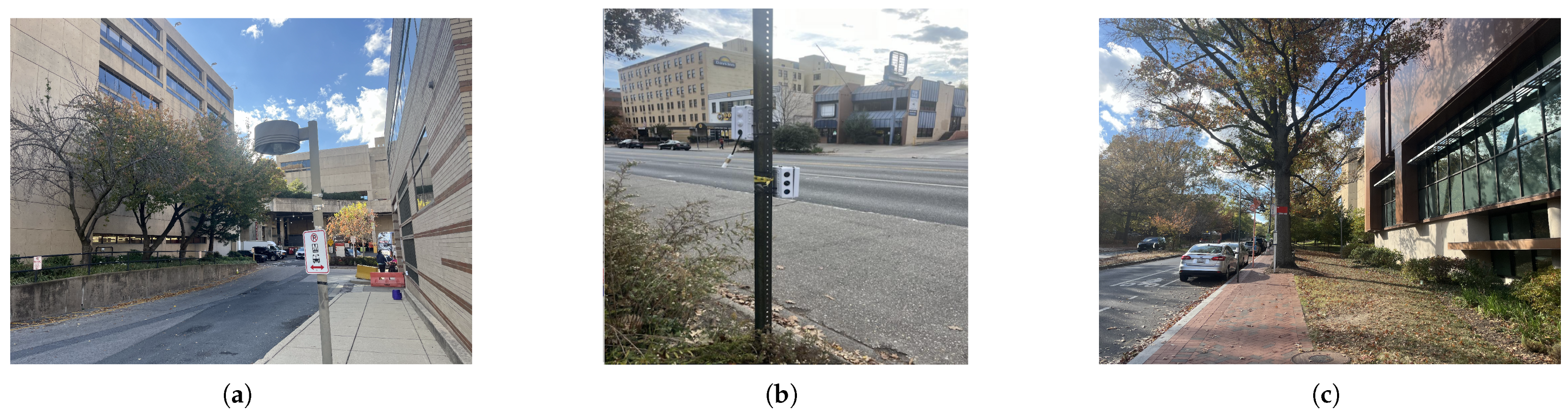
2.1. Experimental Setup

Figure 1 shows the experimental sites under investigation for microclimatic measurements from August to November: Veazey Street NW (38°56′39.75″ N, 77°3′51.50″ W), Connecticut Avenue NW (38°56′51.82″ N, 77°3′54.69″ W), and Van Ness Street NW (38°56′51.82″ N, 77°3′54.69″ W). Figure 1a shows Veazey Street NW is located near the city’s residential core and features low-rise buildings with a height of 10–15 m and street widths ranging from 15–20 m, giving it an H/W ratio of 0.5–0.75. Figure 1b shows Connecticut Avenue NW (38°56′51.82″ N, 77°3′54.69″ W), with taller buildings (20–30 m) and a street width of 10–15 m, has a higher H/W ratio of 1.5–2.0. The dense traffic, both vehicle and pedestrian, along with the compact street design, creates unique microclimatic conditions, leading to temperature shifts and altered wind patterns. Figure 1c shows Van Ness Street NW (38°56′51.82″ N, 77°3′54.69″ W) features buildings between 6–10 m in height, and street widths 20–25 m, with an H/W ratio of 0.3–0.5. This primarily residential area allows for better air circulation compared to the other two streets but still experiences notable pollutant levels due to its traffic.

2.2. Sensor Nodes

The experiment utilized a range of environmental sensors to monitor urban microclimates, with nodes placed at different locations to measure key parameters summarized in Table 1. The sensors included the PMS5003 (Plantower, Beijing, China) for particulate matter (PM1.0 to PM10), the MICS 6814 (SGX Sensortech, Neuchâtel, Switzerland) for gases such as CO, NO2, and NH3, and the SEN0385 (DFRobot, Shanghai, China) for ambient temperature and humidity. Additionally, an ultrasonic wind sensor measured wind speed and direction. Table 1 summarizes the sensors used with their measured parameters, accuracy, and resolution.These sensors were integrated into environmental nodes that were deployed across sites, with each node collecting real-time data for later analysis.
The process of building the sensor nodes began by organizing sensors into two groups based on power requirements and functionality as depicted in Figure 2. High-power sensors, such as the DFRobot Multigas sensor for O3 and the DFRobot Temperature and Humidity Sensor (SEN0385; DFRobot, Shanghai, China), were placed in one group, while low-power sensors, including the PMS5003 (Plantower, Beijing, China) for particulate matter and the MICS-6814 (SGX Sensortech, Neuchâtel, Switzerland) for gases such as CO, NO2, and NH3, were placed in another. This approach helped evaluate each node’s performance while optimizing power consumption between 3.3V and 5V. Lithium batteries, with a capacity of 40 mAh and a runtime of 8–10 h, powered the system.
The first node (Figure 2a) consisted of the PMS5003 and MICS-6814 sensors. In this configuration, a red and orange wires supplied power (VCC), a black wire was used for ground (GND), a yellow wire for data communication, and other colors for control or additional signal lines. The sensors and battery were mounted on a breadboard, with all components connected to the Arduino UNO. The lithium battery connected via red (positive) and black (negative) leads supplied power directly to the board and sensors.
The second node (Figure 2b) included the DFRobot temperature and humidity sensor and the DFRobot gas sensor for ozone (O3). Here, a similar wiring scheme was followed: red wires provided 5V power, black wires were used for ground, and green and blue, and other wires facilitated data transmission between the sensors and Arduino. Each sensor was connected through the breadboard to the microcontroller, and the power was similarly supplied through the lithium battery using red and black lines.
Several studies have employed methodologies similar to our approach in utilizing low-cost sensors for urban air quaity monitoring. Mead et al. [28] examined the use of electromechanical sensors in dense urban networks to monitor air pollutants, highlighting the feasibility and challenges of this deployment. Castell al. [29] assessed the performance of low-cost sensor platforms for air quality monitoring and personal exposure estimation, demonstrating their potential contribution to environmental health studies. Furthermore, Wang et al. [30] conducted a field evaluation of low-cost particulate matter sensors in high-density urban settings, providing insights into their accuracy and reliability for large-scale applications. While these studies underscore the viability of low-cost sensors in air quality monitoring, several challenges remain, including the impact of environmental factors such as humidity and temperature on sensor accuracy, cross sensitivity and interference among different gases (e.g., NO2 and O3), and the need for frequent calibration due to sensor drift over time [31,32,33]. Furthermore, low-cost particle sensors may struggle to accurately detect larger particle matter (PM10) [34].

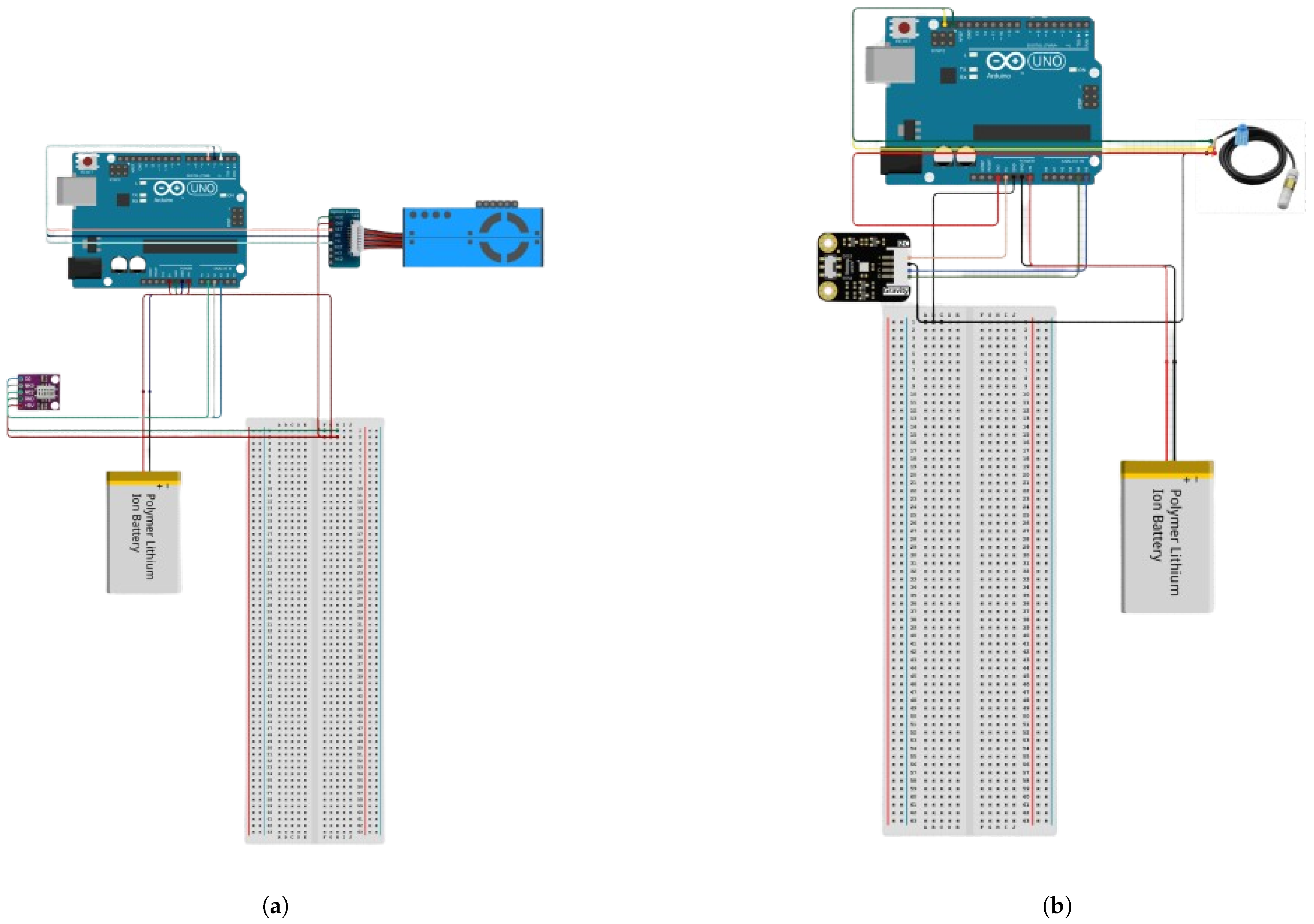
2.2.1. Hardware Description

The data collection system was developed using the Arduino Integrated Development Environment (IDE) version 1.8.19. This software platform, based on the C/C++ programming language, retains key functionalities from earlier versions of the IDE. The system follows a structured process involving hardware initialization, sensor validation, data acquisition, and storage [35]. Initially, the Arduino Uno is configured by defining pin assignments for sensor communication. Digital sensors provide immediate readings, while analog sensors require a brief stabilization period before accurate measurements can be obtained. The system operates in a continuous loop, where sensor data is collected, validated, and processed. Anomalous readings are flagged or discarded to ensure data quality. The validated data is stored in CSV format, making it compatible with MATLAB R2024b and Microsoft Excel V16.89.1 for further analysis. Simultaneously, the ESP-01 Wi-Fi module transmits data wirelessly, while an SD card module ensures local data backup. Connectivity monitoring mechanisms verify the reliability of data transmission and storage. Finally, sensor calibration experiments are conducted before full deployment. Figure 3 illustrates the Arduino Uno process flow for collecting data from the sensor nodes.

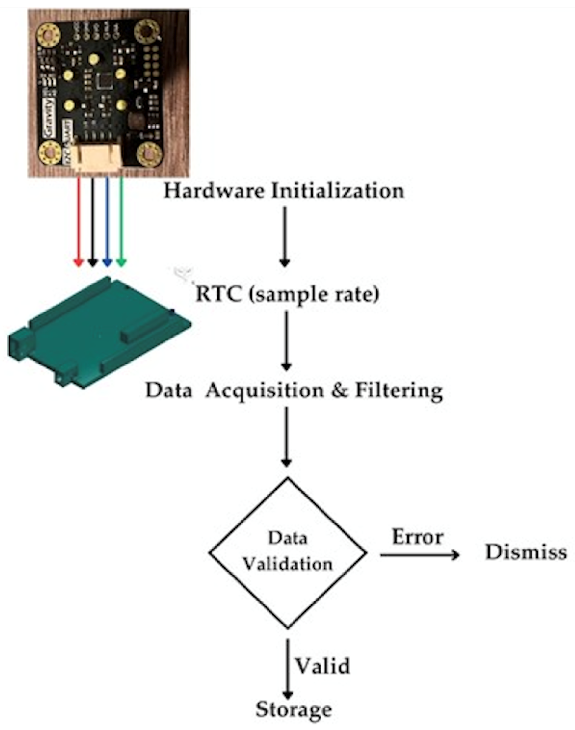
2.2.2. Software Description

The software monitoring interface is designed to collect and display data from multiple environmental sensors, including air quality sensors (NO2, NH3, CO, O3) and a temperature-humidity sensor (SHT3x), while also saving the results to an SD card.

2.2.3. Sensor Calibration Methods

Sensors were calibrated following standard methodologies to ensure data accuracy. The temperature sensor (SEN0385) was cross-referenced with a regulatory-grade instrument. The calibration of the gas sensors (SEN0472, MICS-6814, and PMS5003) followed the reference methodologies outlined in the Environmental Protection Agency (EPA) Air Sensor Guidebook [36]. Baseline corrections and span calibration techniques were employed following best practices from ISO 4225:2020 (Air Quality- General Aspects) [37]. The recorded gas concentrations were also compared to the reference values provided by the U.S. Environmental Protection Agency (EPA) [38].
The calibration of the SEN0385 temperature sensor was conducted by comparing its readings with those from the Ultrasonic Portable Solar Instrument (Calypso Instruments, Zaragoza, Spain), a high-precision reference instrument with an accuracy of ±0.1 °C. The Calypso instrument accounted for environmental variables such as humidity, wind speed, and wind direction, ensuring a comprehensive calibration approach. To refine the sensor’s accuracy, a span calibration was performed, adjusting both the baseline and full-scale response of the SEN0385. A calibration curve was developed by analyzing temperature data from both sensors, ensuring that the SEN0385 readings aligned closely with those from the Calypso reference instrument. This calibration process guarantees that future temperature measurements are accurate, consistent, and corrected for potential environmental variations.
The span calibration process for the DFRobot SEN0472 Ozone (O3) sensor was conducted in a clean indoor environment to ensure accurate ozone measurements. Initially, the sensor was installed and allowed to stabilize. Baseline readings were recorded in a controlled indoor setting (see Figure 4), where ozone concentrations were generally low, typically ranging from 0 to 0.1 ppm, reflecting normal indoor air conditions with minimal external contamination [13]. Since no additional ozone sources were introduced, the ambient ozone concentration naturally served as the reference for calibration. This process involved using baseline readings to develop a calibration curve, adjusting the sensor’s output to align with observed ambient ozone levels, thereby ensuring consistent and reliable future measurements.
Similarly, the calibration of the MICS-6814 gas sensor (for CO and NO2) and the PMS5003 particulate matter sensor followed a comparable span calibration approach. Baseline readings were recorded in the same clean indoor room, where ambient air contained natural concentrations of CO (typically 0.1–0.5 ppm), NO2 (0–0.1 ppm), and PM2.5 (5–15 μ g / m 3 ) [39]. The sensors’ outputs were adjusted based on these baseline measurements, ensuring that their readings accurately reflected ambient indoor air conditions with minimal contamination. This approach aligns with methodologies used in previous sensor calibration studies, emphasizing the importance of establishing sensor-specific calibration functions through controlled colocation with reference instruments [13].

2.3. UHI Index

The Urban Heat Island (UHI) index is a key measure used to assess the temperature difference between urban areas and their surrounding rural environments. It is commonly defined as the difference in temperature between the land surface temperature (LST) of an urban area and that of a rural or suburban area. The UHI index can also be expressed in air temperature between the two areas, reflecting the heat retention and generation within urban environments compared to less developed, rural settings. The basic formula for the UHI index is:
UHI Index = T rural T urban
where T urban represents the temperature of the urban area and T rural is the temperature of the surrounding rural area, both expressed in degrees Celsius (°C) or Kelvin (K). This index is vital for understanding the extent of the UHI effect, as urban areas tend to retain heat due to increased surface roughness, building materials, and human activities, leading to higher temperatures compared to rural areas [40]. To quantify Urban Heat Island (UHI) effects, temperature and wind data from Germantown, M.D., a suburban reference site, were used as a baseline for comparison. This data, obtained from the Open-Meteo Historical Weather [41] represented atmospheric conditions with lower urban influence. This comparison with suburban data provided a means to isolate urban-induced thermal and air quality anomalies.

2.4. Numerical Analysis

To numerically assess the correlation between local microclimate and specific constrains of the area, the numerical model was developed using some measurement data. For thermal comfort evaluation, the Predicted Mean Vote (PMV) index was used, as it considers factors such as air temperature, humidity, wind speed, and clothing, providing a quantitative assessment of thermal comfort [42]. The model was calibrated and validated with real-world data to ensure accuracy.

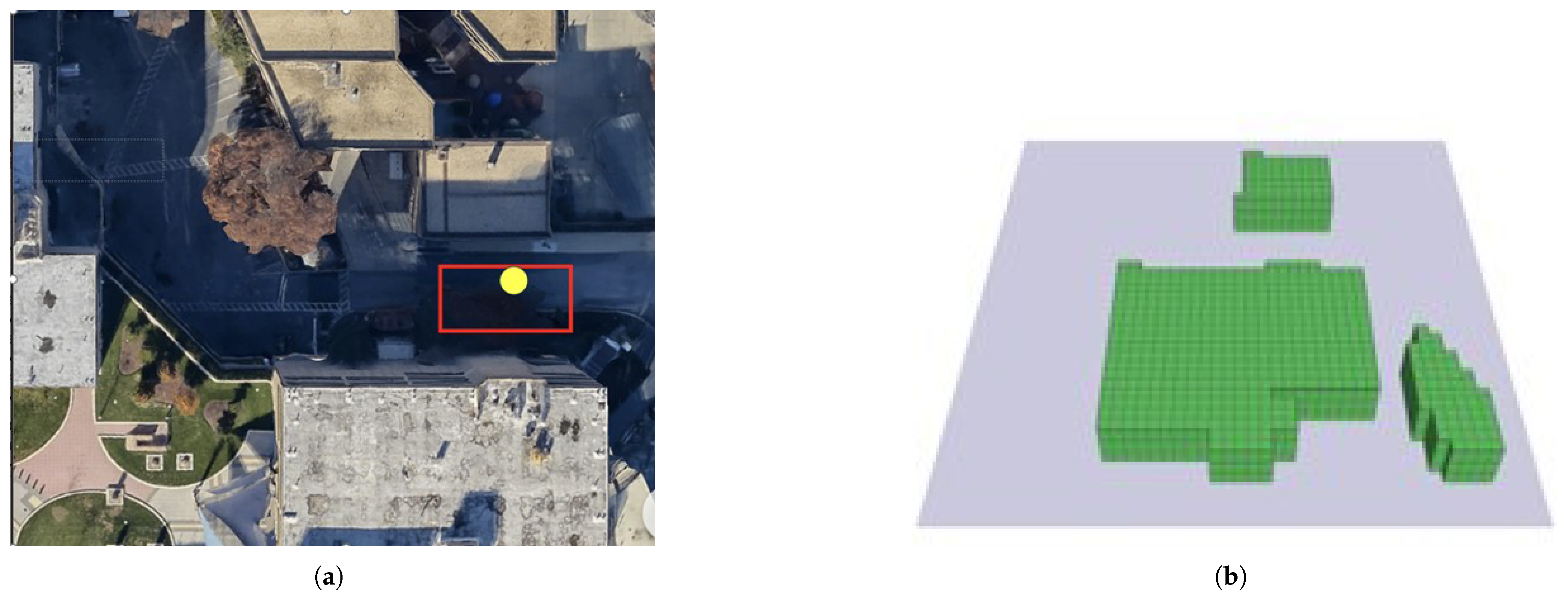
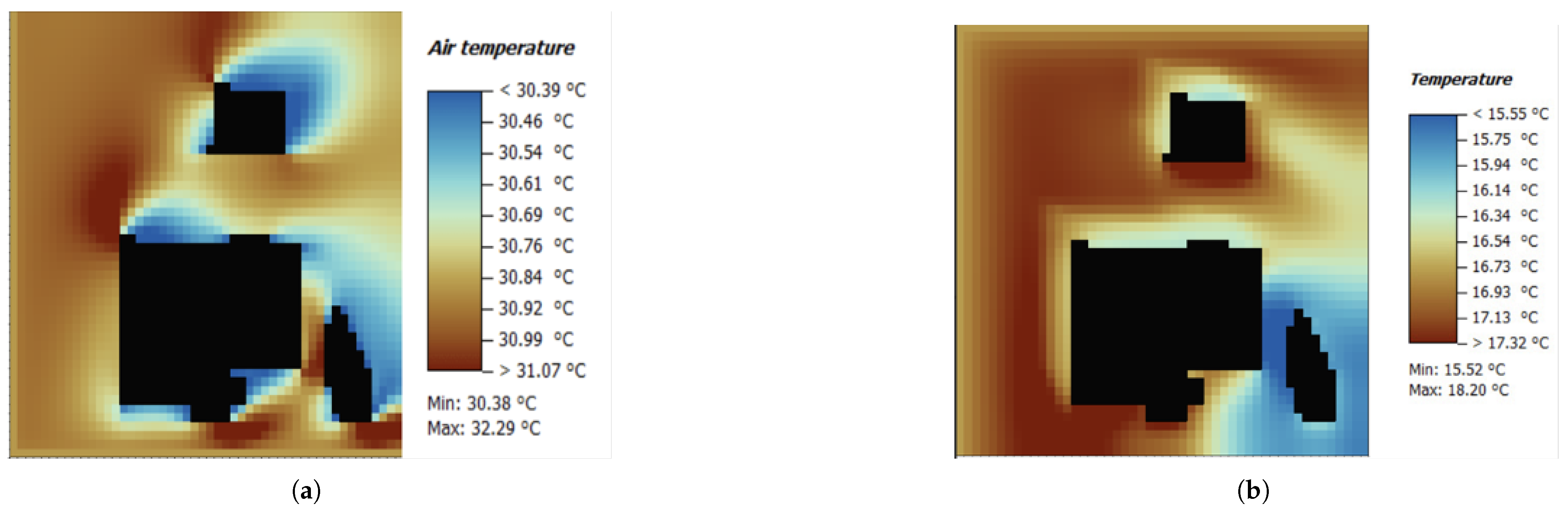
2.4.1. Computational Fluid Dynamics (CFD) Microclimate Modeling

ENVI-met LITE version 5.7.1 was selected due to its ability to accurately resolve environmental variations within the urban canopy layer using a three-dimensional computation fluid dynamics (CFD) approach. The software employs the orthogonal Arakawa C-grid for numerical discretization, which allows fine spatial resolution and incorporates complex topographical and urban features. ENVI-met uses Reynolds-averaged Navier-Strokes (RANS) equations to calculate the wind field, incorporating the Bruse/ENVI-met 2017 Turbulence Kinetic Energy (TKE) model to account for energy distribution and dissipation in the air. The surface temperatures of fades were calculated using a three-node transient state model, and the finite difference method was employed to solve partial differential equations within the system.
Figure 5 presents an aerial view of the Veazey St. NW experimental site. The rectangle outlines the street canyon, while the yellow circle indicates the location of the deployed sensor nodes. This figure illustrates a realistic model of the urban heat area, developed and calibrated using data collected during the initial set of experiments.The calibration and validation process were performed according to the ASHRAE Guideline 14 (ANSI/ASHRAE, 2023) [43] using the data obtained from the environmental and air quality sensors. The model was further refined by incorporating building materials that most closely matched those found at the experimental site. Specifically, the wall materials were modeled with moderate insulation. These simulations allowed for an accurate representation of the UHI effects, including temperature and wind dynamics, and provided an understanding of the interaction between the built environment and atmospheric conditions.
The blueprint model simulations revealed that temperature and wind speed vary with respect to building orientation and height, width between the building surfaces, and wind direction. High elevation buildings are more likely to trap and retain heat than low elevation buildings. Also, narrow street canyons are more likely to experience lower wind speeds than wider street canyons experience. Figure 6 highlights the temperature variation and wind speed, where the highest temperatures were recorded between buildings with the largest H/W ratios (1.5 and 1.2), where temperatures reached 18.2 °C and 16.7 °C, respectively. These areas also experienced the lowest wind speeds, ranging from 0.1 to 0.5 m/s. On the other hand, a building with a smaller H/W ratio of 0.3 resulted in a lower temperature of 15.5 °C, but with significantly higher wind speeds of 6.1 m/s.

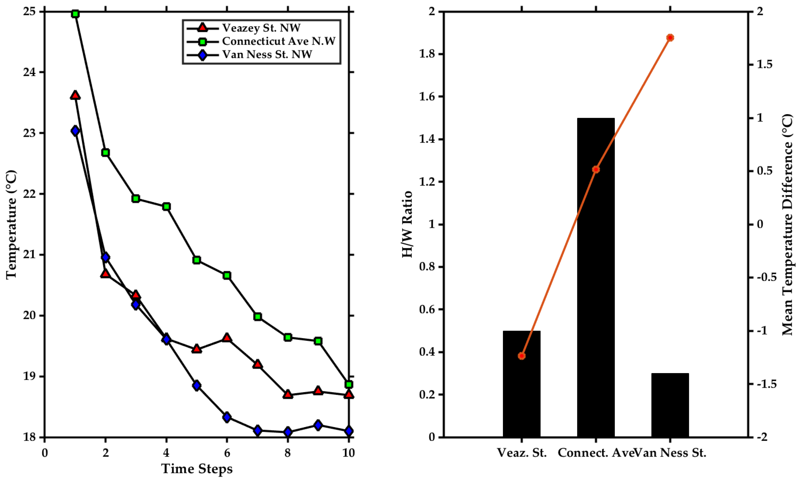
2.4.2. Height-to-Width (H/W) Ratio Analysis

The study also investigated the influence of the height-to-width (H/W) ratio on the microclimatic variability across the experimental sites. The H/W ratio is a critical parameter in urban morphology, as it determines the extent of solar radiation, wind flow, and heat retention within urban canyons [42,44,45]. Table 2 summarizes the H/W ratio of each experimental site calculated based on the building heights and the width of the streets.
The thermo-physical properties of the materials presented in Table 3 were determined based on a combination of literature reviews and commonly accepted data from various sources. The values for walls with moderate insulation were derived from standard construction materials and insulation types commonly used in building design, as found in studies such as those by Pisello et al. [46] and similar research. Asphalt roof and roofing tile properties were sourced from industry-standard material data sheets and studies on building materials’ thermal performance. For greenery, the values were obtained from research on vegetation and its thermal properties, particularly focusing on its role in urban microclimates and heat island mitigation. These values serve as approximations for the materials’ behavior in thermal simulations, ensuring a realistic representation of their performance in urban settings.

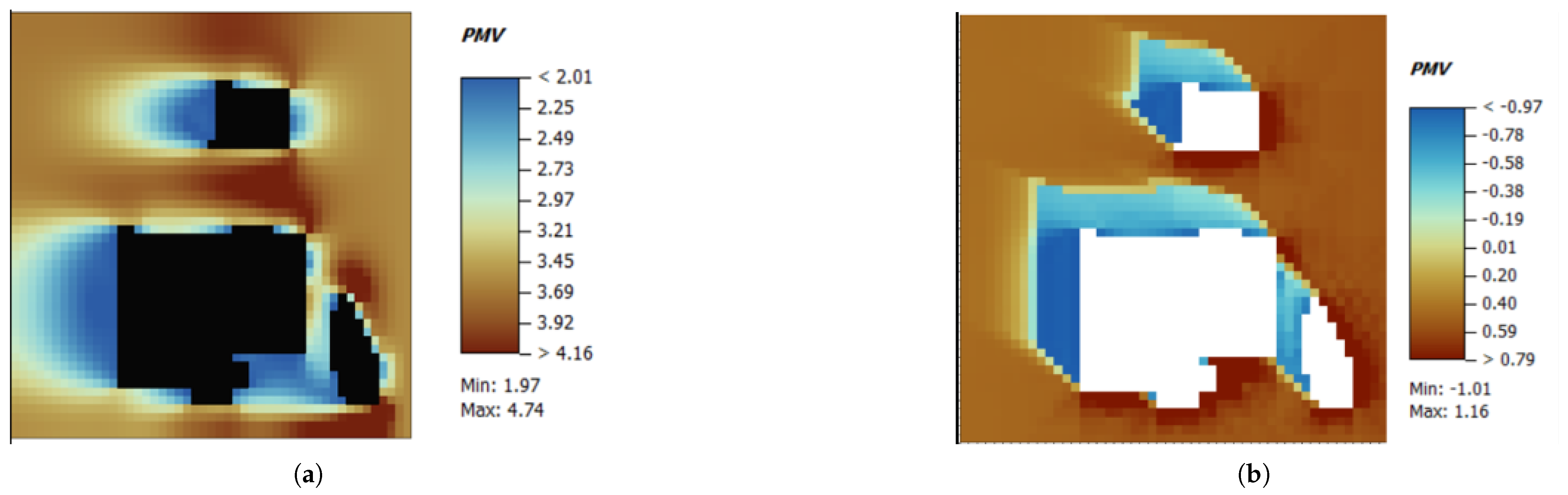
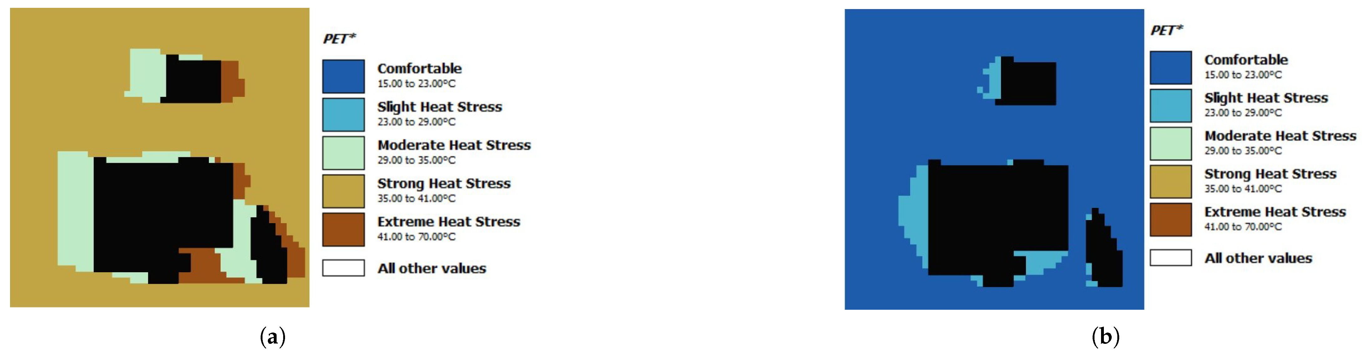
2.5. Thermal Comfort Index

The study incorporated a thermal comfort index analysis using Predicted Mean Vote (PMV) model and the Physiological Equivalent Temperature (PET) as key parameters. The PMV index, developed by Fanger, integrates environmental and physiological factors such as air temperature, humidity [42], wind speed, clothing insulation, and metabolic activity. It is typically calculated using a detailed formula that considers the balance between heat produced by the body and heat lost to the environment. The optimal PMV range for thermal comfort is generally considered to be between −0.5 and +0.5 according to ISO 7730:2005 standards [47], representing a neutral thermal comfort.
The PET index, developed by Höppe, is derived using the Munich Energy Balance Model for individuals (MEMI) and represents air temperature at which the human body maintains heat balance. PET accounts for parameters such as solar radiation, wind speed, humidity, and the thermal resistance of clothing and is usually expressed in degrees Celsius [44]. The optimal PET comfort range in temperate climates such as the one in Washington, D.C. area, typically lies between 18 °C and 23 °C, with values outside this range indicating varying degrees of thermal discomfort.
In this study, simulations for both PMV and PET were conducted using an average female subject with summer clothing (clothing insulation of 0.5 clo) and a metabolic activity of 1.2 met. These indices were applied to assess the thermal comfort of individuals at each experimental site and evaluate the impacts of UHI on residents’ comfort. They also provided critical insights into the correlation between UHI intensity and thermal comfort, supporting microclimate analysis [40,42].

2.6. Data Calibration

To evaluate of the numerical model the following calibration indexes are evaluated [45]:
  • Root Mean Square Error ( R M S E ): Represents the average magnitude of errors between sensor readings and reference (simulation) values. It is expressed as:
    R M S E = 1 n i = 1 n ( y i y ^ i ) 2
    where y i denotes the reference value, y ^ i is the corresponding sensor reading, and n is the total number of observations. A smaller R M S E indicates better accuracy.
  • Correlation Coefficient ( R 2 ): Quantifies the linear relationship between sensor readings and simulation measurements. It is calculated as:
    R 2 = 1 i = 1 n ( y i y ^ i ) 2 i = 1 n ( y i y ¯ ) 2
    where y ¯ is the mean of the reference values. An R 2 value close to 1 indicates a strong positive correlation, meaning the sensor data follows the trends of the simulation results.

3. Results

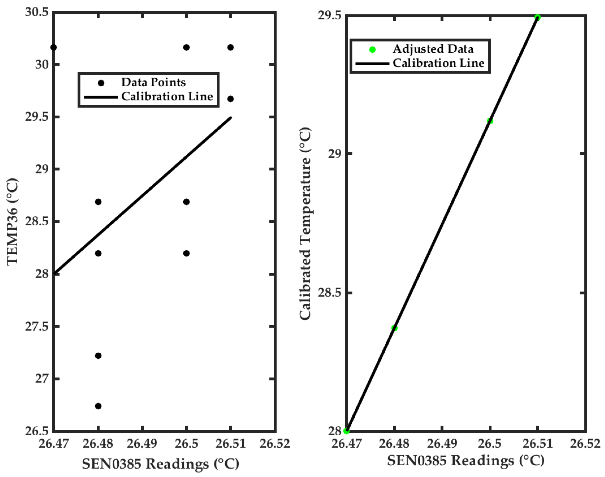
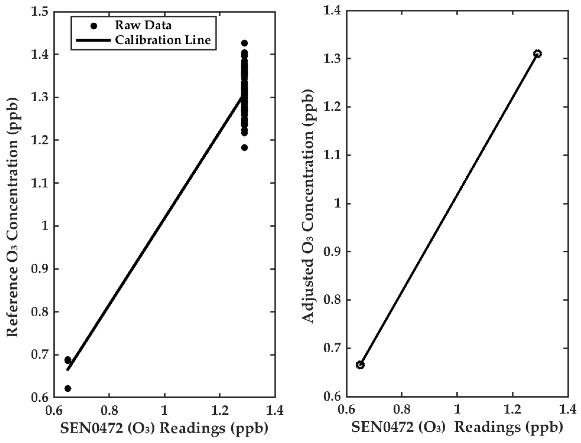
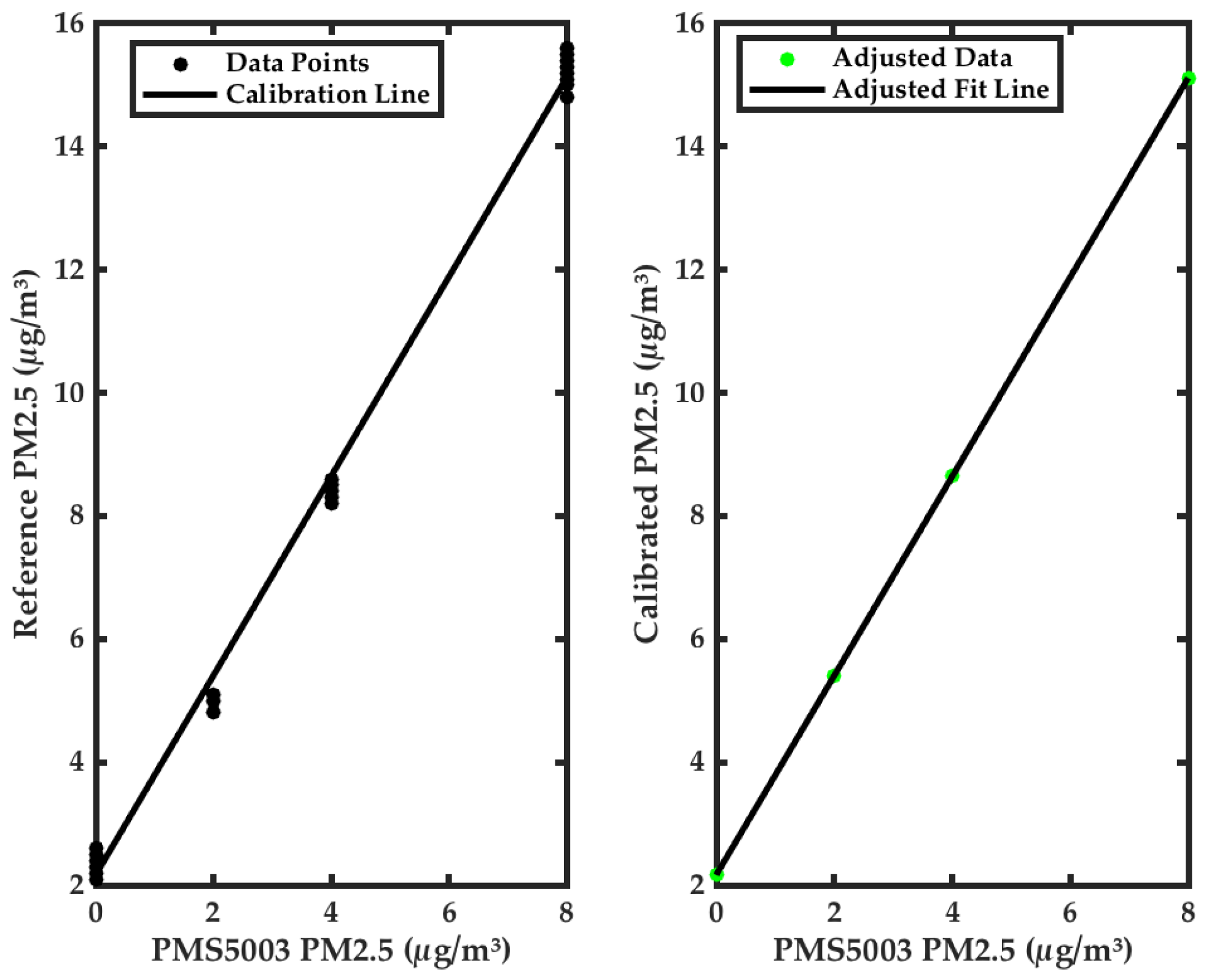
3.1. Sensor Data Calibration

The SEN0385 temperature sensor and the ozone sensor both exhibited lower readings compared to their respective reference instruments, with temperature differences ranging from 0.01 °C to 0.3 °C and ozone variations between 0.65 ppb and 1.3 ppb. Similarly, the MICS 6814 sensor (NO2 and CO) showed discrepancies between reference values. For NO2 raw readings ranged from 0 to 100 ppb (0.1 ppm), while the reference values ranged from 0 to 0.20 ppb (0.020 ppm). The CO raw readings ranged from 4.7 ppm to 4.9 ppm, with the reference values ranging from 1.0 to 5.0 ppm. To correct these biases, a linear model was applied:
T = slope × ( Sensor Reading ) + Intercept
The slopes (0.965 for temperature, 1.002 for O3, 0.066 for NO2, and −13.2 for CO) indicate that for every 1-unit increase in raw sensor readings, the adjusted values increase proportionally, while the intercepts account for minor offsets. Figure 7, Figure 8, Figure 9 and Figure 10 highlight these differences for each sensor, with dashed lines representing the calibration models and the adjusted sensors data after applying corrections.

3.2. UHI Microclimate: Urban Morphology

The relationship between temperature and Height-to-Width (H/W) ratio across the three monitored locations—Veazey St. NW, Connecticut Ave. NW, and Van Ness St. NW show a clear correlation between urban morphology and thermal conditions. Figure 11 illustrates temperature variations from 6 November to 7 November 2024 (21:00–15:00) at the three locations, with each site characterized by a distinct H/W ratio with the red line representing the mean temperature differences between the locations. Connecticut Ave. NW, with the highest H/W ratio range (1.5–2.0), consistently exhibited the highest temperatures, reaching up to 24.9 °C during the evening of 6 November 2024. The wide street layout and minimal shading amplify solar exposure, resulting in elevated thermal conditions. Conversely, Van Ness St. NW, which has the lowest H/W ratio range (0.3–0.5), recorded the lowest temperatures throughout the monitoring period, with values dropping to 18.1 °C during the early hours of 7 November 2024. Veazey St. NW, with a moderate H/W ratio range (0.5–0.75), exhibited intermediate temperature values, ranging between those of Connecticut Ave. NW and Van Ness St. NW. On average, the temperature at Veazey St. NW was 1.5 °C lower than Connecticut Ave. NW but 0.5 °C higher than Van Ness St. NW.

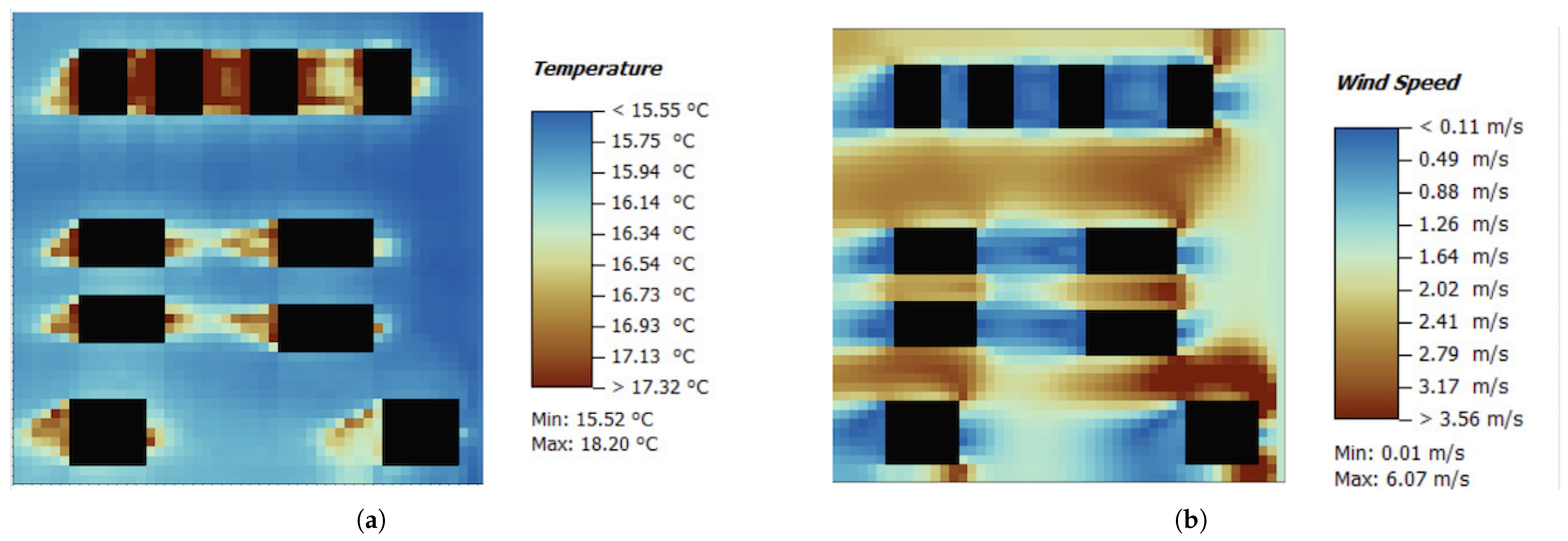
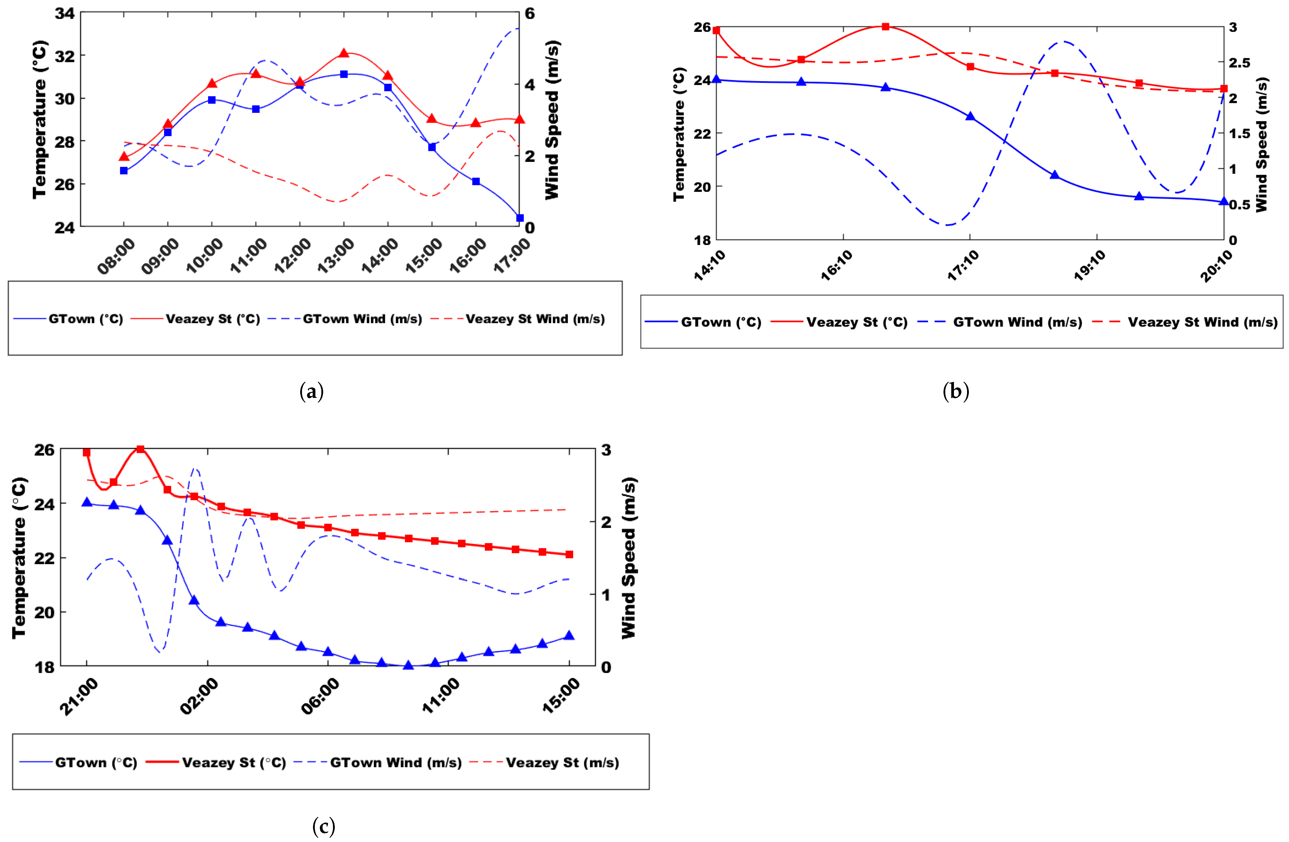
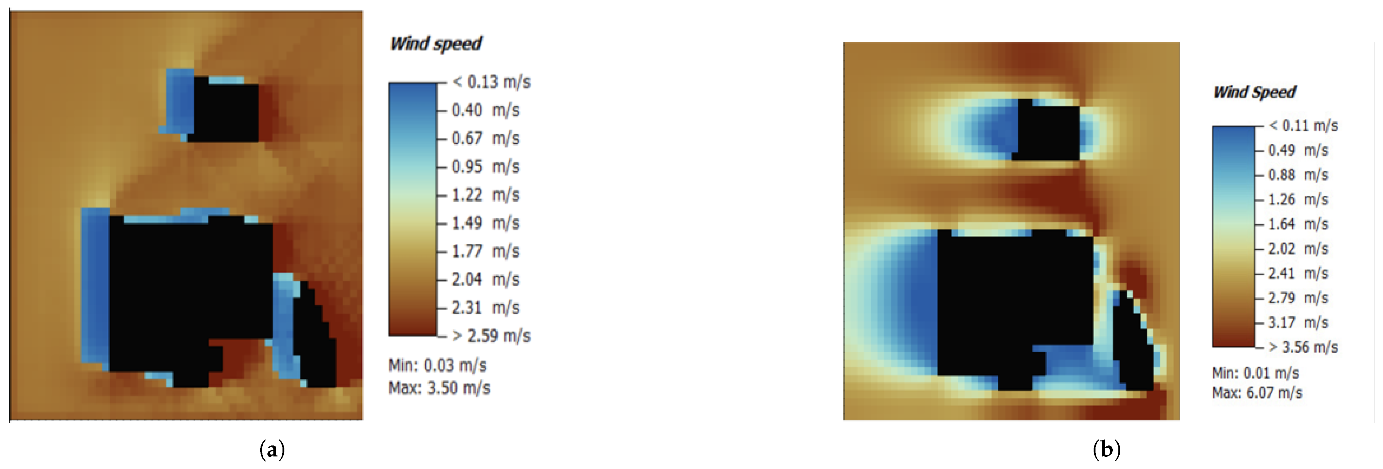
3.2.1. UHI Microclimate Parameters: Temperature and Wind Speed

Figure 12 depicts the temperature and wind fluctuations in Washington, D.C. and Germantown, M.D. On 26 August 2024, during the hours of 15:00 to 16:00, the recorded peak temperatures were 32 °C in Washington, D.C. and 31 °C in Germantown, M.D. Throughout the day, temperatures in Washington, D.C. remained consistently higher than those in Germantown. Additionally, peak wind speeds reached 4.7 m/s at 13:00 in Washington, D.C., compared to 2.7 m/s at 18:30 in Germantown. During the afternoon and evening, wind speeds were consistently higher in Washington, D.C. than in Germantown, M.D.
On 4 October 2024, between 15:00 and 16:00, the peak temperatures recorded were 24 °C in Washington, D.C. and 23 °C in Germantown, M.D. Similar 26 August 2024, temperatures throughout the day were consistently higher in Washington, D.C. Peak wind speeds occurred at 13:00 in Washington, D.C. (3.9 m/s) and at 18:30 in Germantown (2.5 m/s). Again, wind speeds in Washington, D.C. were observed to be consistently greater than those in Germantown during the afternoon and evening.
On 6 November 2024, between 21:00 and 23:00, temperatures ranged from 20.4 °C to 17.7 °C in Germantown, M.D., and from 23.6 °C to 20.3 °C at Veazey St NW, indicating warmer conditions in Washington, D.C. Wind speeds ranged from 1.6 m/s to 2.2 m/s in Germantown, whereas they were significantly higher at Veazey St NW, ranging from 3.07 m/s to 3.12 m/s.
On 7 November 2024, temperatures in Germantown, M.D. ranged from 16.8 °C at 6:00 to 23.8 °C at 12:00. At Veazey St NW, temperatures ranged slightly higher, from 18.7 °C to 24.1 °C. Wind speeds in Germantown varied from 1.6 m/s to 4.5 m/s, with the highest speed occurring at 13:00. At Veazey St NW, wind speeds ranged from 1.7 m/s to 3.8 m/s. Notably, during the afternoon, wind speeds were higher in Germantown, M.D. compared to Veazey St NW.

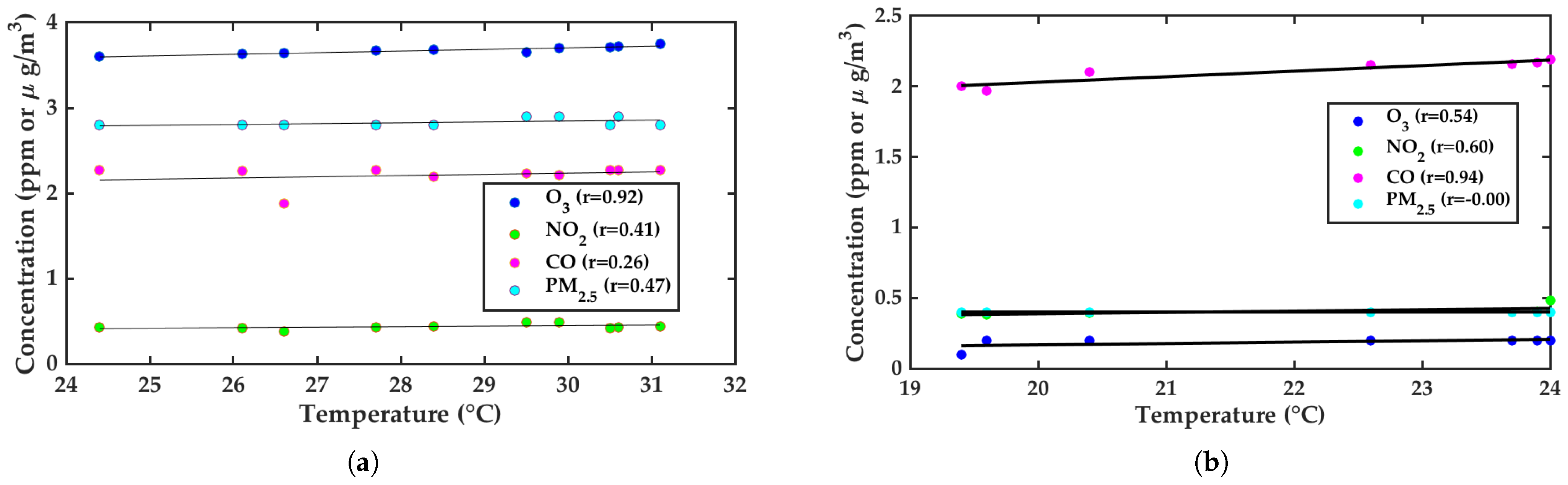
3.2.2. UHI Microclimate Parameters and Pollutant Concentration

Figure 13 illustrates the correlation between temperature and the concentrations of Ozone (O3), Nitrogen Dioxide (NO2), Carbon Monoxide (CO), and PM2.5 on 26 August 2024 and 4 October 2024. On 26 August 2024, The temperature ranged from 24.4 °C to 31.1 °C, peaking in the afternoon and cooling towards the evening. O3 concentrations fluctuated between 3.6 ppb and 7.3 ppb, showing a weak positive correlation (r = 0.92) with temperature. NO2 concentrations ranged from 0.3 ppm to 0.4 ppm, with a moderate positive correlation (r = 0.41) to temperature, peaking in the afternoon as temperatures increased. CO levels remained relatively stable between 1.9 ppm and 2.3 ppm, showing a weak positive correlation (r = 0.26) with temperature. PM2.5 concentrations were stable at around 2.8 µg/m³, with little variation and a weak positive correlation (r = 0.47) to temperature. On 4 October 2024, the temperature ranged from 19.4 °C to 24 °C, gradually decreasing as evening approached. O3 concentrations remained stable at 3.6 ppb initially and then decreased to 1.8 ppb, showing a weak positive correlation (r = 0.54) with temperature. NO2 concentrations ranged from 0.4 ppm to 0.5 ppm, showing a positive correlation to temperature (r = 0.60). CO levels fluctuated between 1.9 ppm and 2.2 ppm, showing a strong relationship to temperature (r = 0.94). PM2.5 concentrations remained constant at 0.4 μ g/m3, with no correlation to temperature (r = 0.00).

3.3. Numerical Analysis

On 26 August 2024, simulations indicated high air temperatures, low wind speeds, and considerable thermal discomfort in the study area, particularly in areas between buildings with limited airflow. In contrast, the evening and early morning hours of 6–7 November 2024, exhibited significantly cooler temperatures, greater wind variability, and more favorable thermal conditions.
Figure 14 illustrates the temperature distribution for both days. On 26 August, temperatures ranged from 30.4 °C to 32.3 °C, with the highest values occurring around the airflow-restricted zones between buildings. In contrast, temperatures on 6–7 November were lower, peaking at 19.4 °C, reflecting cooler conditions during the evening and early morning hours. Figure 15 presents the wind speed variations for both dates. On 26 August, wind speeds ranged from 0.03 m/s to 3.50 m/s, indicating calm conditions that hindered natural cooling. During the 6–7 November period, wind speeds exhibited greater variation, ranging from 0.01 m/s to 6.07 m/s, showing increased variability and enhanced cooling during the night.
Figure 16 shows the PMV values for both days. On 26 August, PMV values ranged from 1.97 to 4.74, suggesting significant discomfort, which could lead to increased sweating and heat accumulation for the average pedestrian due to high temperatures and limited wind flow. Conversely, on 6–7 November, PMV values ranged from −1.01 to 1.16, indicating cooler conditions and less heat stress for pedestrians. The PET values ranged from 35 °C to 41 °C at the simulated experimental site on 26 August, signaling that the average pedestrian experienced discomfort due to the higher thermal load. Alternatively, the PET values on 6–7 November ranged from 15 °C to 23 °C, suggesting more comfortable thermal conditions for the average pedestrian (see Figure 17).

Data Validation: R M S E , R 2

The validation of the experimental and simulated results for air temperature and wind speed shows a strong agreement between the two datasets, as summarized in Table 4. For 26 August, the simulated air temperature ranged between 30.1 °C and 32.1 °C, closely matching the experimental range of 30.4 °C to 32.3 °C, with an R M S E of 0.75 and an R 2 of 0.91. Similarly, the simulated wind speed (0.02–3.20 m/s) aligns well with the experimental values (0.03–3.50 m/s), yielding an R M S E of 0.38 and an R 2 of 0.86. During the 6–7 November evening period, the maximum simulated temperature (19.40 °C) closely matches the experimental maximum (19.45 °C), with an R M S E of 0.62 and an R 2 of 0.94, indicating high accuracy. The wind speed comparison for this period also shows good agreement, with simulated values ranging from 0.03 to 4.10 m/s compared to the experimental range of 0.04 to 4.50 m/s, resulting in an R M S E of 0.42 and an R 2 of 0.88.

4. Discussion

The results confirm the significant influence of urban morphology on microclimate dynamics, particularly highlighting the role of high height-to-width (H/W) ratios in exacerbating urban heat and air quality challenges. Computational Fluid Dynamics (CFD) simulations, coupled with experimental validation, demonstrated a strong correlation between urban design parameters and microclimatic conditions. For instance, on 26 August, simulated air temperatures (30.1 °C–32.1 °C) closely matched experimental measurements (30.4 °C–32.3 °C), with a root mean square error R M S E of 0.75 and a correlation coefficient R2 of 0.91. This high level of agreement underscores the reliability of the CFD model in capturing temperature variations influenced by urban morphology. Similarly, wind speed simulations (0.02–3.20 m/s) were consistent with observed values (0.03–3.50 m/s), yielding an R M S E of 0.38 and an R2 of 0.86, further confirming the model’s ability to replicate wind dynamics in urban environments. Comparable accuracy was observed in November, where simulated temperatures (19.1 °C–19.4 °C) aligned closely with experimental values (19.4 °C), achieving an R M S E of 0.62 and an R2 of 0.94. Despite the high accuracy, some discrepancies between simulated and experimental results were attributed to the omission of critical parameters such as Land Surface Temperature (LST), Albedo, and Sky View Factor. These factors are known to influence heat absorption, reflection, and emission, and their exclusion led to minor deviations in the model’s predictions. Addressing these omissions in future studies could further refine the model’s precision.
The findings also reveal that areas with higher H/W ratios experienced elevated temperatures, reduced wind speeds, and poorer air quality. During the summer period, PM2.5 levels averaged 2.8 μ g/m3, and ozone (O3) ranged from 1.8 to 7.3 ppb, indicating pollutant accumulation in densely built environments. These results support the hypothesis that compact urban designs, characterized by high H/W ratios, retain heat and restrict ventilation, amplifying the urban heat island (UHI) effect and deteriorating air quality. The behavior of each pollutant further substantiates this conclusion. On 26 August 2024, when temperatures ranged from 24.4 °C to 31.1 °C, O3 concentrations increased markedly alongside rising temperatures, as reflected in a strong positive correlation ( r = 0.92 ). This suggests that higher temperatures enhance photochemical reactions that generate ozone, especially under stagnant wind conditions typical of dense urban forms. NO2 also showed a moderate positive correlation ( r = 0.41 ), indicating that traffic emissions and heat-induced chemical activity contributed to elevated afternoon concentrations. CO, with a weaker correlation ( r = 0.26 ), appeared less sensitive to temperature changes, likely due to its emission being more directly tied to traffic patterns than atmospheric processes. PM2.5 concentrations remained relatively stable around 2.8 μ g/m3, showing only a weak correlation ( r = 0.47 ), implying that fine particulate matter was influenced more by local sources and atmospheric dispersion than by temperature alone.
On 4 October 2024, with cooler temperatures ranging from 19.4 °C to 24.0 °C, O3 levels dropped, and its correlation with temperature weakened ( r = 0.54 ), confirming reduced photochemical activity in cooler conditions. Interestingly, NO2 demonstrated a stronger correlation ( r = 0.60 ), suggesting that in cooler but still stable conditions, pollutant accumulation was more affected by limited dispersion. CO exhibited a significantly strong correlation ( r = 0.94 ), possibly due to cooler conditions limiting vertical mixing and allowing vehicular emissions to build up near the ground. In contrast, PM2.5 remained constant at 0.4 μ g/m3 with no correlation ( r = 0.00 ), indicating either cleaner atmospheric conditions or effective dispersion mechanisms during that period.
Additionally, the results highlight the strong influence of urban microclimate variations on thermal comfort, emphasizing the role of urban geometry and ventilation. On 26 August, both PMV (1.97–4.74) and PET (35 °C–41 °C) values indicate severe heat stress, driven by high temperatures, limited airflow, and urban heat retention. This suggests that densely built environments with poor ventilation amplify discomfort, potentially affecting pedestrian well-being and outdoor activity levels. In contrast, the lower PMV (−1.01 to 1.16) and PET (15 °C–23 °C) values on 6–7 November demonstrate significantly improved comfort due to cooler temperatures and better thermal conditions. The alignment between PMV and PET values underscores their reliability in assessing urban thermal environments.

5. Conclusions

Urban morphology plays a crucial role in shaping microclimate dynamics, with high height-to-width (H/W) ratios shown to increase temperatures, restrict ventilation, and worsen air quality. The strong alignment between CFD simulations and experimental data, evidenced by low RMSE values and high correlation coefficients, demonstrates the effectiveness of modeling techniques in capturing urban thermal and wind dynamics. Compact urban designs with higher H/W ratios were found to intensify the urban heat island (UHI) effect, contributing to elevated pollutant levels due to reduced airflow. Conversely, areas with lower H/W ratios demonstrated improved ventilation and reduced pollutant accumulation, emphasizing the importance of optimizing urban geometry to mitigate UHI effects. The Predicted Mean Vote (PMV) and Physiological Equivalent Temperature (PET) indexes further highlighted the impact of urban design on thermal comfort, reinforcing the need for sustainable planning strategies that prioritize better airflow and reduced thermal stress in urban environments.
Future investigations should prioritize the deployment of pedestrian-level sensing systems to enhance the understanding of urban microclimate variations. These systems, equipped with advanced sensors for real-time monitoring of temperature, humidity, wind speed, and air pollutants such as PM2.5, CO, and NO2, can provide high-resolution data at the human scale. Such localized measurements will allow for better validation of simulation models and a deeper exploration of microclimatic differences influenced by factors like pedestrian activity, traffic, and urban design. Additionally, integrating pedestrian-level data with IoT frameworks and machine learning algorithms could enhance urban climate modeling and support targeted interventions to improve air quality, thermal comfort, and overall urban resilience. This approach offers a promising pathway to developing smarter, healthier, and more adaptive urban spaces.

Author Contributions

Conceptualization, M.D. and L.K.M.; methodology, M.D.; software, L.K.M.; validation, M.D.; formal analysis, M.D., H.A. and K.K.R.; investigation, L.K.M.; resources, M.D. and L.K.M.; data curation, L.K.M.; writing—original draft preparation, L.K.M.; writing—review and editing, M.D. and L.K.M.; visualization, M.D. and P.B.; supervision, M.D.; project administration, M.D.; funding acquisition, M.D. All authors have read and agreed to the published version of the manuscript.

Funding

This research was sponsored by the Army Research Laboratory and was accomplished under Cooperative Agreement Number W911NF-19-2-0120. The views and conclusions contained in this document are those of the authors and should not be interpreted as representing the official policies, either expressed or implied, of the Army Research Laboratory or the U.S. Government. The U.S. Government is authorized to reproduce and distribute reprints for government purposes notwithstanding any copyright notation herein.

Data Availability Statement

The data supporting the findings of this study are available from various sources referenced in the literature, including urban microclimate, urban heat island (UHI) data, thermal imagery, and air quality measurements. These sources include books such as Urban Heat Island Mitigation by Santamouris, articles from journals like Environmental Pollution, Urban Climate, and websites such as the U.S. Environmental Protection Agency (EPA) and ENVI-met. Additionally, data can be accessed through environmental research platforms like the European Environment Agency (EEA) and government databases such as the U.S. National Aeronautics and Space Administration (NASA), the National Oceanic and Atmospheric Administration (NOAA), and the U.S. Department of Energy’s (DOE) Energy Information Administration (EIA).

Conflicts of Interest

The authors declare no conflicts of interest. The funders had no role in the design of the study; in the collection, analyses, or interpretation of data; in the writing of the manuscript; or in the decision to publish the results.

References

  1. Jabbar, H.K.; Hamoodi, M.N.; Al-Hameedawi, A.N. Urban heat islands: A review of contributing factors, effects and data. IOP Conf. Ser. Earth Environ. Sci. 2023, 1129, 012038. [Google Scholar] [CrossRef]
  2. Akbari, H.; Pomerantz, M.; Taha, H. Cool surfaces and shade trees to reduce energy use and improve air quality in urban areas. Sol. Energy 2001, 70, 295–310. [Google Scholar] [CrossRef]
  3. Santamouris, M. Recent progress on urban overheating and heat island research. Integrated assessment of the energy, environmental, vulnerability and health impact. Synergies with the global climate change. Energy Build. 2020, 207, 109482. [Google Scholar] [CrossRef]
  4. Kang, H.; Zhu, B.; de Leeuw, G.; Yu, B.; van der A, R.J.; Lu, W. Impact of urban heat island on inorganic aerosol in the lower free troposphere: A case study in Hangzhou, China. Atmos. Chem. Phys. 2022, 22, 10623–10634. [Google Scholar] [CrossRef]
  5. He, B.J.; Ding, L.; Prasad, D. Urban ventilation and its potential for local warming mitigation: A field experiment in an open low-rise gridiron precinct. Sustain. Cities Soc. 2020, 55, 102028. [Google Scholar] [CrossRef]
  6. Pusede, S.E.; Steiner, A.L.; Cohen, R.C. Temperature and Recent Trends in the Chemistry of Continental Surface Ozone. Chem. Rev. 2015, 115, 3898–3918. [Google Scholar] [CrossRef]
  7. Gober, P.; Brazel, A.; Quay, R.; Myint, S.W.; Grossman-Clarke, S.; Miller, A.; Rossi, S. Using Watered Landscapes to Manipulate Urban Heat Island Effects: How Much Water Will It Take to Cool Phoenix? J. Am. Plann. Assoc. 2009, 76, 109–121. [Google Scholar] [CrossRef]
  8. Santamouris, M. Heat island research in Europe: The state of the art. Adv. Build. Energy Res. 2007, 1, 123–150. [Google Scholar] [CrossRef]
  9. Cao, J.; Zhou, W.; Zheng, Z.; Ren, T.; Wang, W. Within-city spatial and temporal heterogeneity of air temperature and its relationship with land surface temperature. Landsc. Urban Plan. 2021, 206, 103979. [Google Scholar] [CrossRef]
  10. Weng, Q.; Lu, D.; Schubring, J. Estimation of land surface temperature–vegetation abundance relationship for urban heat island studies. Remote Sens. Environ. 2004, 89, 467–483. [Google Scholar] [CrossRef]
  11. Voogt, J.A.; Oke, T.R. Thermal remote sensing of urban climates. Remote Sens. Environ. 2003, 86, 370–384. [Google Scholar] [CrossRef]
  12. Kavian Nezhad, M.; RahnamayBahambary, K.; Lange, C.; Fleck, B. Modified accuracy of RANS modeling of urban pollutant flow within generic building clusters using a high-quality full-scale dispersion dataset. Sustainability 2023, 15, 14317. [Google Scholar] [CrossRef]
  13. Liu, M.; Barkjohn, K.; Norris, C.; Schauer, J.; Zhang, J.; Zhang, Y.; Hu, M.; Bergin, M. Using low-cost sensors to monitor indoor, outdoor, and personal ozone concentrations in Beijing, China. Environ. Sci. Process. Impacts 2020, 22, 131–143. [Google Scholar] [CrossRef]
  14. Bruse, M.; Fleer, H. Simulating surface–plant–air interactions inside urban environments with a three dimensional numerical model. Environ. Model. Softw. 1998, 13, 373–384. [Google Scholar] [CrossRef]
  15. Kong, F.; Yin, H.; James, P.; Hutyra, L.; He, H. Effects of spatial pattern of greenspace on urban cooling in a large metropolitan area of eastern China. Landsc. Urban Plan. 2014, 128, 35–47. [Google Scholar] [CrossRef]
  16. Yang, X.; Zhao, L.; Bruse, M.; Meng, Q. Evaluation of a microclimate model for predicting the thermal behavior of different ground surfaces. Build. Environ. 2013, 60, 93–104. [Google Scholar] [CrossRef]
  17. Toparlar, Y.; Blocken, B.; Maiheu, B.; van Heijst, G. A review on the CFD analysis of urban microclimate. Renew. Sustain. Energy Rev. 2017, 80, 1613–1640. [Google Scholar] [CrossRef]
  18. Radhi, H. On the effect of global warming and the UAE built environment. In Global Warming; Harris, S.A., Ed.; IntechOpen: Rijeka, Croatia, 2010; pp. 95–110. [Google Scholar]
  19. Salim, S.; Ong, K.; Cheah, S. Comparison of RANS, URANS and LES in the prediction of airflow and pollutant dispersion. In Proceedings of the World Congress on Engineering and Computer Science, San Francisco, CA, USA, 19–21 October 2011; Volume 2, pp. 19–21. [Google Scholar]
  20. Blocken, B.; Carmeliet, J. Pedestrian wind environment around buildings: Literature review and practical examples. J. Therm. Envel. Build. Sci. 2004, 28, 107–159. [Google Scholar] [CrossRef]
  21. Schaefer, T.; Kieslinger, B.; Fabian, C. Citizen-based air quality monitoring: The impact on individual citizen scientists and how to leverage the benefits to affect whole regions. Citiz. Sci. Theory Pract. 2020, 5, 6. [Google Scholar] [CrossRef]
  22. Malings, C. Integrating low-cost sensor systems and networks to enhance air quality applications. In Proceedings of the India Clean Air Summit (ICAS), Bengaluru, India, 26–30 August 2024. [Google Scholar]
  23. Lu, T.; Chen, C. Uncertainty evaluation of humidity sensors calibrated by saturated salt solutions. Measurement 2007, 40, 591–599. [Google Scholar] [CrossRef]
  24. Dubovikov, N.; Podmurnaya, O. Measuring the relative humidity over salt solutions. Meas. Tech. 2001, 44, 1260–1261. [Google Scholar] [CrossRef]
  25. Eggert, G. Saturated salt solutions in showcases: Humidity control and pollutant absorption. Herit. Sci. 2022, 10, 54. [Google Scholar] [CrossRef]
  26. Mijling, B.; Jiang, Q.; De Jonge, D.; Bocconi, S. Field calibration of electrochemical NO2 sensors in a citizen science context. Atmos. Meas. Tech. 2018, 11, 1297–1312. [Google Scholar] [CrossRef]
  27. Antoniou, N.; Montazeri, H.; Neophytou, M.; Blocken, B. CFD simulation of urban microclimate: Validation using high-resolution field measurements. Sci. Total Environ. 2019, 695, 133743. [Google Scholar] [CrossRef]
  28. Mead, M.; Popoola, O.; Stewart, G.; Landshoff, P.; Calleja, M.; Hayes, M.; Baldovi, J.; McLeod, M.; Hodgson, T.; Dicks, J.; et al. The use of electrochemical sensors for monitoring urban air quality in low-cost, high-density networks. Atmos. Environ. 2013, 70, 186–203. [Google Scholar] [CrossRef]
  29. Castell, N.; Dauge, F.R.; Schneider, P.; Vogt, M.; Lerner, U.; Fishbain, B.; Broday, D.; Bartonova, A. Can commercial low-cost sensor platforms contribute to air quality monitoring and exposure estimates? Environ. Int. 2017, 99, 293–302. [Google Scholar] [CrossRef]
  30. Wang, S.; Ma, Y.; Wang, Z.; Wang, L.; Chi, X.; Ding, A.; Yao, M.; Li, Y.; Li, Q.; Wu, M.; et al. Mobile monitoring of urban air quality at high spatial resolution by low-cost sensors: Impacts of COVID-19 pandemic lockdown. Atmos. Chem. Phys. 2021, 21, 7199–7215. [Google Scholar] [CrossRef]
  31. Hayward, I.; Martin, N.; Ferracci, V.; Kazemimanesh, M.; Kumar, P. Low-cost air quality sensors: Biases, corrections and challenges in their comparability. Atmosphere 2024, 15, 1523. [Google Scholar] [CrossRef]
  32. Bauerová, P.; Šindelářová, A.; Rychlík, Š.; Novák, Z.; Keder, J. Low-cost air quality sensors: One-year field comparative measurement of different gas sensors and particle counters with reference monitors at Tušimice observatory. Atmosphere 2020, 11, 492. [Google Scholar] [CrossRef]
  33. Clements, A.; Reece, S.; Conner, T.; Williams, R. Observed data quality concerns involving low-cost air sensors. Atmos. Environ. X 2019, 3, 100034. [Google Scholar] [CrossRef]
  34. Molina Rueda, E.; Carter, E.; L’Orange, C.; Quinn, C.; Volckens, J. Size-resolved field performance of low-cost sensors for particulate matter air pollution. Environ. Sci. Technol. Lett. 2023, 10, 247–253. [Google Scholar] [CrossRef] [PubMed]
  35. Martinez, A.; Hernandez-Rodríguez, E.; Hernandez, L.; Schalm, O.; González-Rivero, R.A.; Alejo-Sánchez, D. Design of a low-cost system for the measurement of variables associated with air quality. IEEE Embed. Syst. Lett. 2022, 15, 105–108. [Google Scholar] [CrossRef]
  36. U.S. Environmental Protection Agency. Enhanced Air Sensor Guidebook; U.S. Environmental Protection Agency: Washington, DC, USA, 2022.
  37. ISO 4225:2020; Air Quality—General Aspects—Vocabulary. International Organization for Standardization: Geneva, Switzerland, 2020. Available online: https://www.iso.org/standard/72525.html (accessed on 13 December 2024).
  38. U.S. Environmental Protection Agency. Download Daily Data; U.S. Environmental Protection Agency: Washington, DC, USA, 2025.
  39. Nguyen, N.; Nguyen, H.; Le, T.; Vu, C. Evaluating low-cost commercially available sensors for air quality monitoring and application of sensor calibration methods for improving accuracy. Open J. Air Pollut. 2021, 10, 1. [Google Scholar] [CrossRef]
  40. Oke, T.R. The energetic basis of the urban heat island. Q. J. R. Meteorol. Soc. 1982, 108, 1–24. [Google Scholar] [CrossRef]
  41. Open-Meteo. Open-Meteo: Free Weather API for Non-Commercial Use. Open-Meteo.com. 2025. Available online: https://open-meteo.com/ (accessed on 17 May 2025).
  42. Fanger, P. Thermal Comfort: Analysis and Applications in Environmental Engineering; Danish Technical Press: Copenhagen, Denmark, 1970. [Google Scholar]
  43. ASHRAE. ASHRAE Guideline 14-2023 – Measurement of Energy, Demand and Water Savings. Am. Soc. Heat. Refrig. Air Cond. Eng. 2023. [Google Scholar]
  44. Höppe, P. The physiological equivalent temperature–a universal index for the biometeorological assessment of the thermal environment. Int. J. Biometeorol. 1999, 43, 71–75. [Google Scholar] [CrossRef]
  45. Salata, F.; Golasi, I.; de Lieto Vollaro, R.; de Lieto Vollaro, A. Urban microclimate and outdoor thermal comfort. A proper procedure to fit ENVI-met simulation outputs to experimental data. Sustain. Cities Soc. 2016, 26, 318–343. [Google Scholar] [CrossRef]
  46. Pisello, A.; Castaldo, V.; Rossi, F.; Cotana, F. Cool clay tiles in Italian residential districts: Investigation of the coupled thermal-energy and environmental effects. Environ. Sci. Sustain. Dev. 2016, 1, 1–13. [Google Scholar] [CrossRef]
  47. ISO 7730:2005; Ergonomics of the Thermal Environment—Analytical Determination and Interpretation of Thermal Comfort Using Calculation of the PMV and PPD Indices and Local Thermal Comfort Criteria. ISO: Geneva, Switzerland, 2005. Available online: https://www.usgbc.org/resources/iso-7730%E2%80%932005-ergonomics-thermal-environment-analytical-determination-and-interpretation-t (accessed on 17 May 2025).
Figure 1. (a) Veazey St NW; (b) Connecticut Ave NW; (c) Van Ness St NW.
Environments 12 00184 g001
Figure 2. (a) Ozone (O3) and temperature node; (b) gase (CO, NO2, NH3) and particulate matter (PM) node.
Environments 12 00184 g002
Figure 3. Flowchart of Arduino UNO data collection process.
Environments 12 00184 g003
Figure 4. Indoor calibration setup.
Environments 12 00184 g004
Figure 5. (a) Veazey St NW aerial view; (b) Veazey St. NW 3-D simulation (ENVI-met).
Environments 12 00184 g005
Figure 6. Blueprint model simulations: (a) temperature variation; (b) wind distribution.
Environments 12 00184 g006
Figure 7. SEN0385 calibration: raw vs. calibrated data and adjusted readings.
Environments 12 00184 g007
Figure 8. SEN0472 (O3) calibration: raw vs. calibrated data and adjusted readings.
Environments 12 00184 g008
Figure 9. MICS-6814 calibration: raw vs. calibrated Data and adjusted readings.
Environments 12 00184 g009
Figure 10. PMS5003 PM2.5: raw vs. calibrated Data and adjusted readings.
Environments 12 00184 g010
Figure 11. Temperature variation across experimental sites: (left) Temporal trends; (right) H/W ratio comparison.
Environments 12 00184 g011
Figure 12. Temperature (°C) vs. wind speed (m/s) variations: (a) 26 August 2024; (b) 4 October 2024; (c) 6–7 November 2024.
Environments 12 00184 g012
Figure 13. Correlation between gases and temperature (°C): (a) 26 August 2024; (b) 4 October 2024.
Environments 12 00184 g013
Figure 14. CFD simulations of temperature (°C): (a) 26 August 2024; (b) 6–7 November 2024.
Environments 12 00184 g014
Figure 15. CFD simulations of wind speed(m/s): (a) 26 August 2024; (b) 6–7 November 2024.
Environments 12 00184 g015
Figure 16. CFD simulations of PMV: (a) 26 August 2024; (b) 6–7 November 2024.
Environments 12 00184 g016
Figure 17. CFD simulations of PET: (a) 26 August 2024; (b) 6–7 November 2024.
Environments 12 00184 g017
Table 1. Sensor specifications.
Sensor 1Measured ParametersResolutionAccuracy
PMS5003PM1.0, PM2.5, PM100.1 µg/m³±10% or ±1 µg/m³
MICS 6814 (Gas Sensor)CO, NO2, NH30.1 ppm±5% of reading or ±1 ppm
SEN0472O30.1 ppm±5% of reading or ±1 ppm
SEN0385Temperature, Humidity0.1 °C (Temp), 1% (Humidity)±0.3 °C (Temperature), ±3% (Humidity)
Ultrasonic Portable Solar Wind Instrument (Calypso)Wind Speed, Wind Direction, Humidity0.1 m/s (Wind Speed)±2% (Wind Speed), ±3° (Wind Direction)
1 Accuracy values are provided by sensor manufacturers.
Table 2. Building Height, Street Width, and H/W Ratio for Different Locations.
LocationBuilding Height (m) 2Street Width (m) 2H/W Ratio
Veazey St NW10–1515–200.5–0.75
Connecticut Ave NW20–3010–151.5–2.0
Van Ness St6–1020–250.3–0.5
2 Building heights and street widths were measured using Google Maps.
Table 3. Thermo-physical properties of the materials in the case study area.
ElementPropertyValue
Walls (with moderate insulation)Thermal Conductivity (W/m·K)0.35–0.45
Density (kg/m3)600–900
Specific Heat (J/kg·K)1000–1200
Asphalt RoofThermal Conductivity (W/m·K)0.9–1.2
Density (kg/m3)2200–2400
Specific Heat (J/kg·K)1000–1300
Roofing TileThermal Conductivity (W/m·K)0.8–1.5
Density (kg/m3)1400–1600
Specific Heat (J/kg·K)800–1000
Greenery (grass, typical vegetation)Thermal Conductivity (W/m·K)0.2–0.5
Density (kg/m3)50–400
Specific Heat (J/kg·K)1500–2000
Table 4. Data Validation Summary.
ParameterExperimental RangeSimulated RangeRMSER2
Air temperature (°C) 26 August30.38–32.2930.12–32.100.750.91
6–7 November19.4519.10–19.400.620.94
Wind Speed (m/s) 26 August0.03–3.500.02–3.200.380.86
6–7 November0.04–4.500.03–4.100.420.88
Disclaimer/Publisher’s Note: The statements, opinions and data contained in all publications are solely those of the individual author(s) and contributor(s) and not of MDPI and/or the editor(s). MDPI and/or the editor(s) disclaim responsibility for any injury to people or property resulting from any ideas, methods, instructions or products referred to in the content.

