Definition and Validation of Vineyard Management Zones Based on Soil Apparent Electrical Conductivity and Altimetric Survey

Abstract

In the current context of increasing costs of production factors, it is essential to optimize the management of available resources, seeking to incorporate technologies that improve knowledge of the variables involved in the agronomic production process. The aim of this study is to define and validate management zones (MZ) in a 3.3 ha vineyard located near Évora, in the South of Portugal. A contact sensor (“Veris 2000 XA”) was used to map soil apparent electrical conductivity (EC_a) and a precision altimetric survey of the field was carried out with a global navigation satellite system receiver (GNSS). The results of these surveys were submitted to geostatistical treatments that allowed the definition of three MZ (less, intermediate, and more productive potential). The validation of such MZ was carried out by laboratory analysis of soil samples (texture, pH, organic matter—OM, moisture content, phosphorous, potassium, exchange bases, and cation exchange capacity—CEC), measurements of soil compaction (cone index—CI) with an electronic cone penetrometer, and through indices (Normalized Difference Vegetation Index—NDVI, and Normalized Difference Water Index—NDWI) obtained by remote sensing (RS) using Sentinel-2 satellite images. All these parameters (soil parameters and RS indices) proved the validity of the MZ (of less, intermediate, and more productive potential) defined from the EC_a and altimetric survey. This validation attests to the interest of expeditious technological tools for monitoring EC_a as a fundamental step in implementing smart agronomic decision-making processes.

1. Introduction

One of the main challenges for the agricultural sector, and in particular, viticulture, is to adapt to climate change while ensuring the quality of production and its sustainability [1]. Within this context, compounded by rising input costs, it is essential to optimize the management of available resources, by incorporating technologies that provide information on the variables involved in the agronomic production process. This perspective is within the framework of Precision Agriculture (PA), which has expanded in the last decade to practically all crops.

The main goal of Precision Viticulture (PV) is to assess the spatial variability of physiological needs of the vines belonging to different areas of the vineyard in order to implement the management techniques in a more site- and time-specific manner, reducing the use of production factors and, consequently, the environmental impact and maximizing the yield and quality of production [2].

The spatial variability of grapevine (Vitis vinifera L.) within a single vineyard is a relevant issue for growers and winemakers [3], essential for making management decisions [4,5]. A very diverse set of management decisions are required in this crop, ranging from input management (irrigation, fertilizing, spraying) up to cultural practices (pruning, shoot and cluster thinning, canopy management, inter-row cover, or segmented harvesting) [3].

Within-field variability of vine development and, consequently, grape yield and composition, is the result of both spatial and temporal variation of many factors, including edaphic, biological, climatic, topographic, and anthropogenic [4]. Many studies have shown and quantified the existence of significant variability within the vineyards [6]. Knowing the spatial variability of soil characteristics allows a better understanding of the variability of the physiological response of the vines [2]. This variability can be surveyed using a regular sampling grid [6], however, given the cost and time required for this type of sampling and the necessity of many soil samples to achieve an effective spatial representation of any soil property, it cannot be considered a viable and practical process at farm level [7,8]. The use of sensors is becoming the norm for mapping the relevant soil properties, thus reducing the number of soil samples needed to describe field variability [9].

Some factors responsible for variability in a vineyard remain stable over time, such as topography and some soil properties; therefore, the knowledge of their spatial variability can provide a better understanding of this complex decision-making scenario [3] and the definition of management zones (MZ). These represent subfield areas with homogeneous characteristics, such as texture, topography, or nutrient levels [7], and may be used to adapt viticulture practices [5]. The ability to map the spatial variability in vine and soil characteristics allows grape growers to move from a random sampling approach to a smart sampling methodology based on sampling zones of uniform vine characteristics [10]. This can be considered the first step in the application of site-specific crop management [7]. Understanding the spatial variability of factors that influence crop yield is essential to the application of site-specific management [11].

This new possibility of considering perspective of spatial variability is a consequence of the technological means made available by PV to the farm manager [2,10]. These spatially enabled digital technologies provide the possibility of gathering georeferenced spatial datasets [2], information with high spatial resolution (small areas within the field) and great flexibility in the timing of data acquisition, and managing these areas differentially [4,10]. The importance of remote and proximal sensing as tools for smart viticulture application has been evidenced in several reviews published in the last two decades [10].

Variation in soil and topography is likely to have a large impact on vineyard variability [10]. The proximal monitoring of soil variability includes the use of a wide range of sensors [2]. The apparent soil electrical conductivity (EC_a) sensing technology, mounted on mobile platforms and coupled with GNSS receivers, are highly relevant when designing new vineyards and redeveloping existing vineyards [10], but also for the definition of MZ and site-specific management [7]. There are two types of sensors currently on the market to measure soil EC_a based on the method of measurement: contact or non-contact. The first type (e.g., Veris sensor) is invasive and uses electrodes, usually in the shape of coulters that make contact with the soil, generating electrical currents in the soil with an electrode and then measuring the potential difference thanks to a second receiver electrode, which measures the electrical resistivity (i.e., the inverse of conductivity). The second type (e.g., Dualem or EM38 sensors) is non-invasive and is composed of a transmitter and a receiver coil usually installed at opposite ends of a non-conductive bar. This sensor type works on the principle of electromagnetic induction: it generates a magnetic field that induces an electric current in the soil, which in turn creates a second magnetic field proportional to its conductivity, which is measured by the sensor [2,7]. The EC_a is usually related to various soil physical and chemical properties across a wide range of soils [12], such as texture and depth, water retention capacity, organic matter content, salinity [2], cation exchange capacity (CEC), pH, exchangeable magnesium, and other soil nutrients [9].

Another electronic sensor that can help to characterize soil spatial variability and, consequently, its productive potential is the cone penetrometer [13,14]. This measures the cone index (CI, in kPa), which reflects soil compaction and is considered an important tool for the diagnosis of the most restrictive soil layers for root growth at depth [15]. For these reasons, it can be a very interesting parameter in terms of validating MZ.

Other new technologies have made it possible to characterize the crop vegetative vigor. In the last years, several works have shown the potential of remote sensing (RS) in crop monitoring, in particular the vineyard [9,10,16]. The significant impact of soil on vine nutrition and development has led researchers to associate the EC_a maps with vegetation indexes maps to assess the field spatial variability [9,17]. For example, the normalized difference vegetation index (NDVI) can be used to evaluate plant photosynthetic activity and, therefore, its canopy vigor, as well as crop yield and grape quality characteristics [8,10,16]. On the other hand, the normalized difference water index (NDWI) can be used to evaluate plant water stress and leaf water content during growth phases [16]. These vegetation indices have been successfully used by several teams to delineate areas with homogeneous vigor within vineyards for the purpose of site-specific management [3,9,17,18].

This study aims (i) to assess the soil spatial variability of a vineyard through EC_a survey with a contact sensor; (ii) to evaluate the temporal stability of EC_a measurements; (iii) to define MZ based on geostatistical treatment of EC_a and topographic survey; and (iv) to validate MZ by several approaches (soil laboratory analysis, CI and RS indices).

2. Materials and Methods

Figure 1 summarizes, schematically and chronologically, the methodology used in this study to monitor the spatial variability of a vineyard and define and validate MZ. The study was conducted between May 2022 and April 2023.

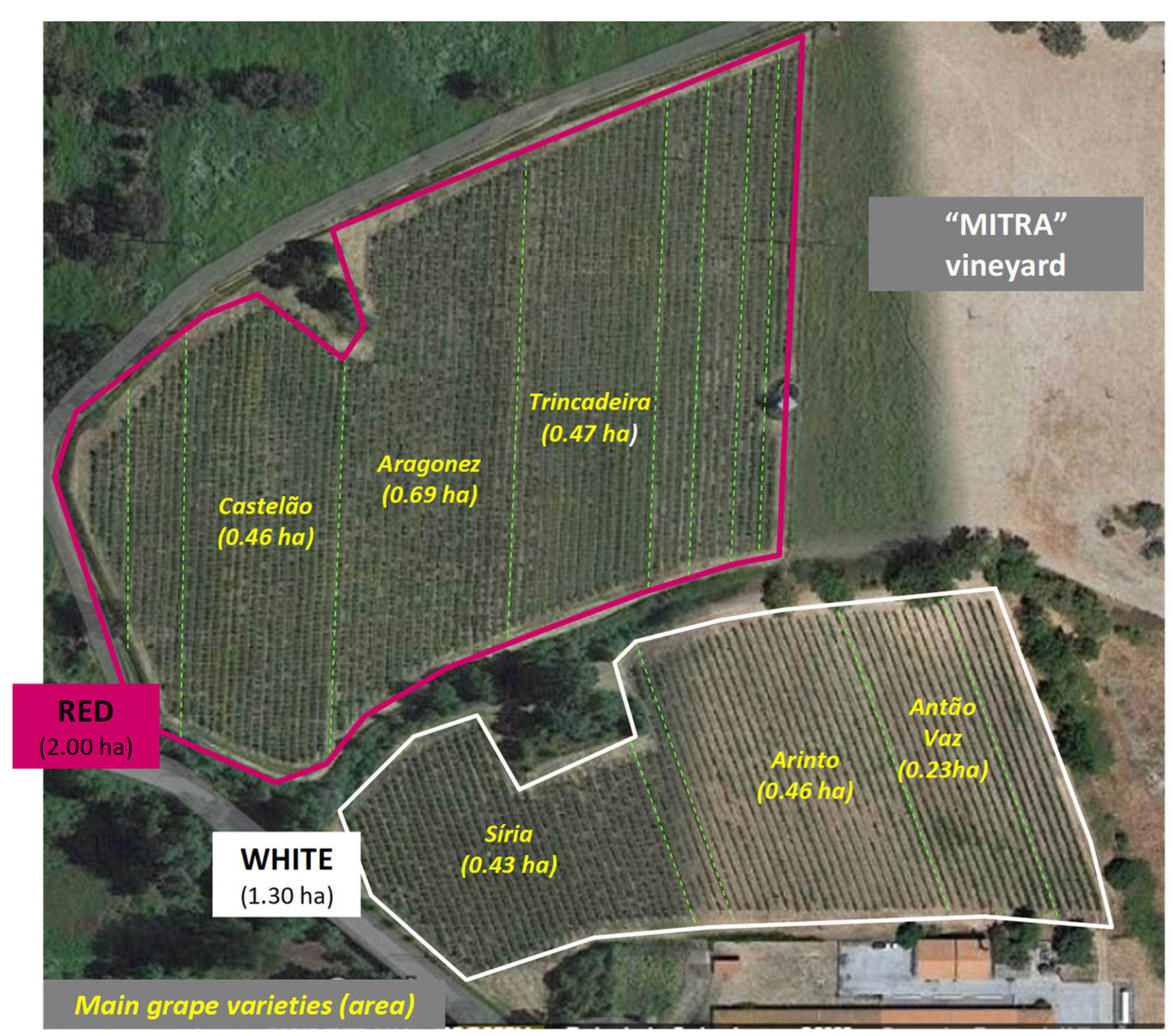
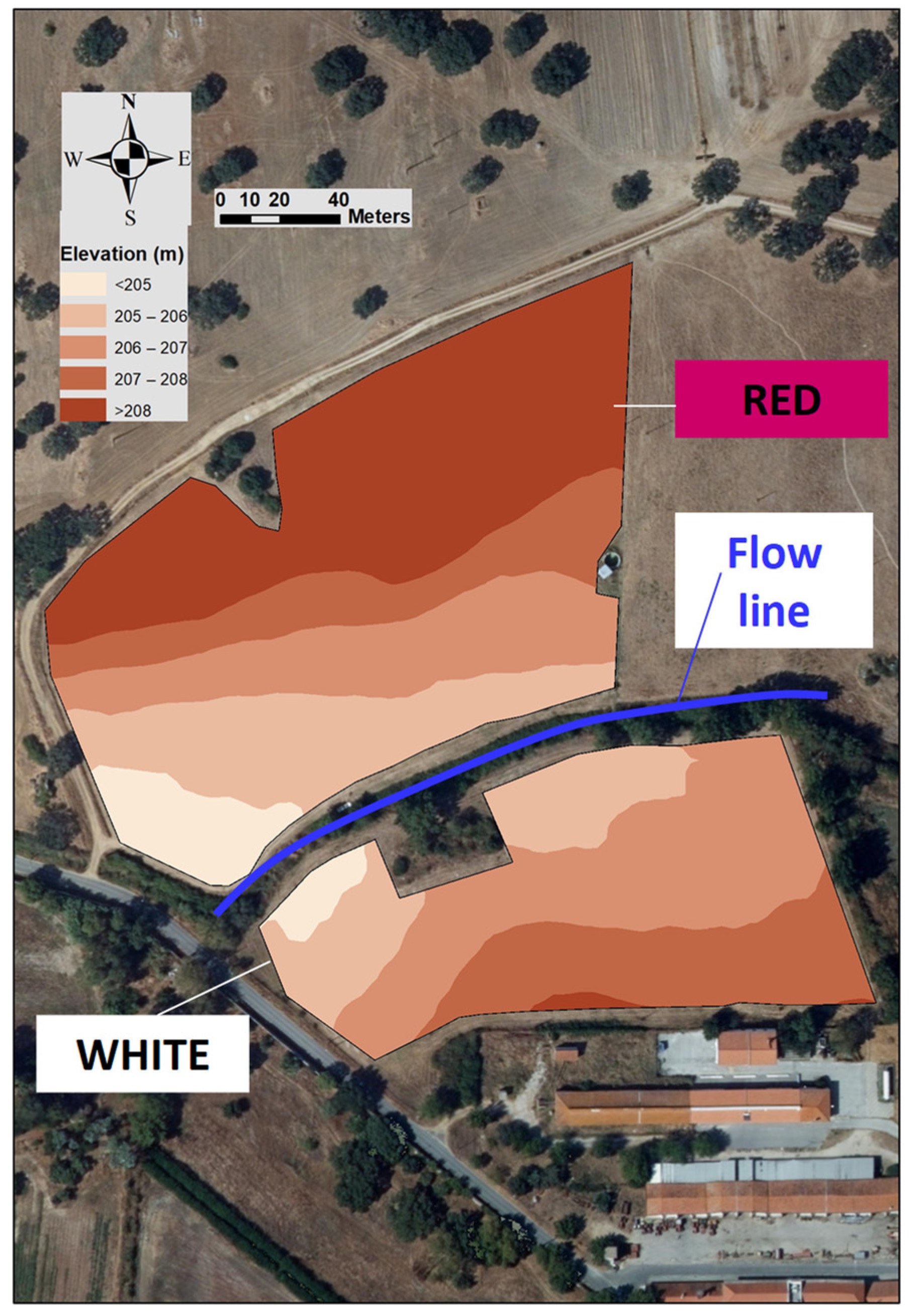
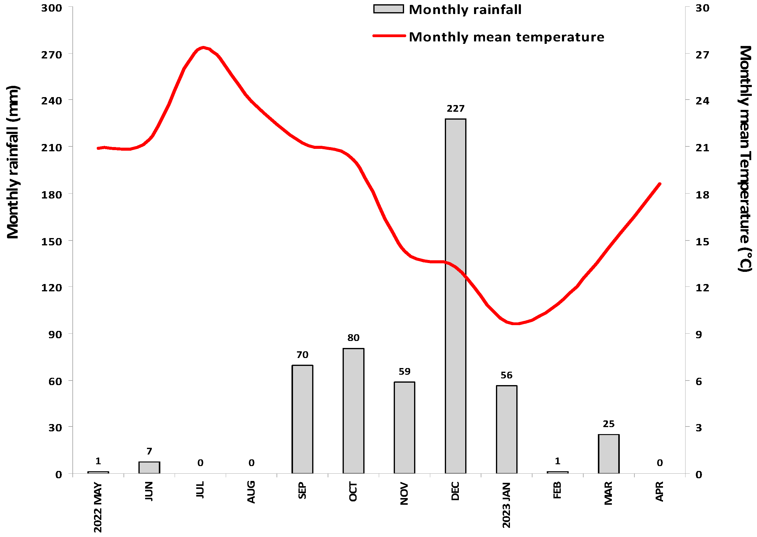
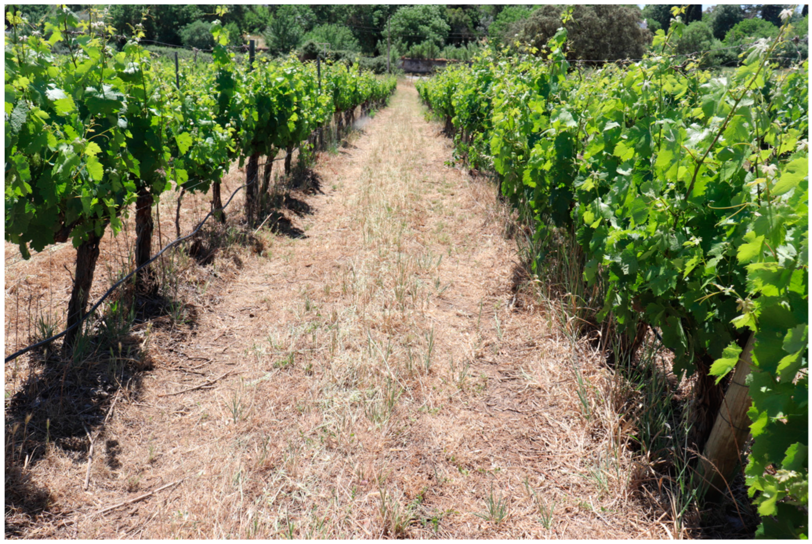
2.1. Study Area

The study field is a 3.3 ha vineyard, located at the “Mitra” farm of “University of Évora” (38.532° N; 8.015° W). The aerial image of the Mitra vineyard (Figure 2) shows two areas: (i) white grapes (1.30 ha, about 85% of which is planted with three varieties: “Arinto”, “Síria”, and “AntãoVaz”) and (ii) red grapes (2.0 ha, about 82% of which is planted with three varieties: “Aragonez”, “Trincadeira”, and “Castelão”). Despite this variability, the information available on the vineyard management history indicates uniform cultural operations (pruning, fertilization, irrigation, phytosanitary treatments, etc.).

A precision altimetric survey of the field was carried out during October 2022 using a real-time kinematic (RTK) GPS instrument (Trimble RTK/PP-4700 GPS manufactured by TRIMBLE Navigation Limited, USA). The altimetric map (Figure 3) was generated using the triangulated irregular network interpolation tool, converted into a grid surface with a 1 m grid resolution using the Spatial Analyst Tools of ArcGIS (version 10.5, ESRI, Inc., Redlands, California, USA). The two sub-fields (“white”, “W” and “red”, R) show a gradual gradient (from South to North in the “W” area and from North to South in the “R” area), and slopes that converge to a flow line, which represents the lowest elevation of the study area.

The dominating soil type of the study area is Cambisol with a granite origin [19], characterized by little or no profile differentiation, slight or moderate weathering of parent material, and by absence of appreciable quantities of illuviated clay and organic matter. Acid Cambisols are not very fertile and are mainly dedicated to mixed agro-silvo-pastoral systems. Cambisols in undulating or hilly terrain (mainly colluvial) are planted to a variety of annual and perennial crops or are used as grazing land. The study area also includes hydromorphic soils and Luvisols. In the Mediterranean region, the often-eroded hills are used for extensive grazing or planted to tree crops [19].

The climate of this Mediterranean region is classified as Csa (Köppen–Geiger classification) [20] and is characterized by high inter-annual irregularity and low rainfall (<600 mm). The thermo-pluviometric diagram of the Évora meteorological station in the year under study (between May 2022 and April 2023; Figure 4) shows an accumulated precipitation of 526 mm, concentrated mainly (98%) in six months (September–January, and March), and the remaining six months with practically no precipitation (February and April–August). In this period without precipitation, particularly between May and August, the average temperature is around 20–30 °C.

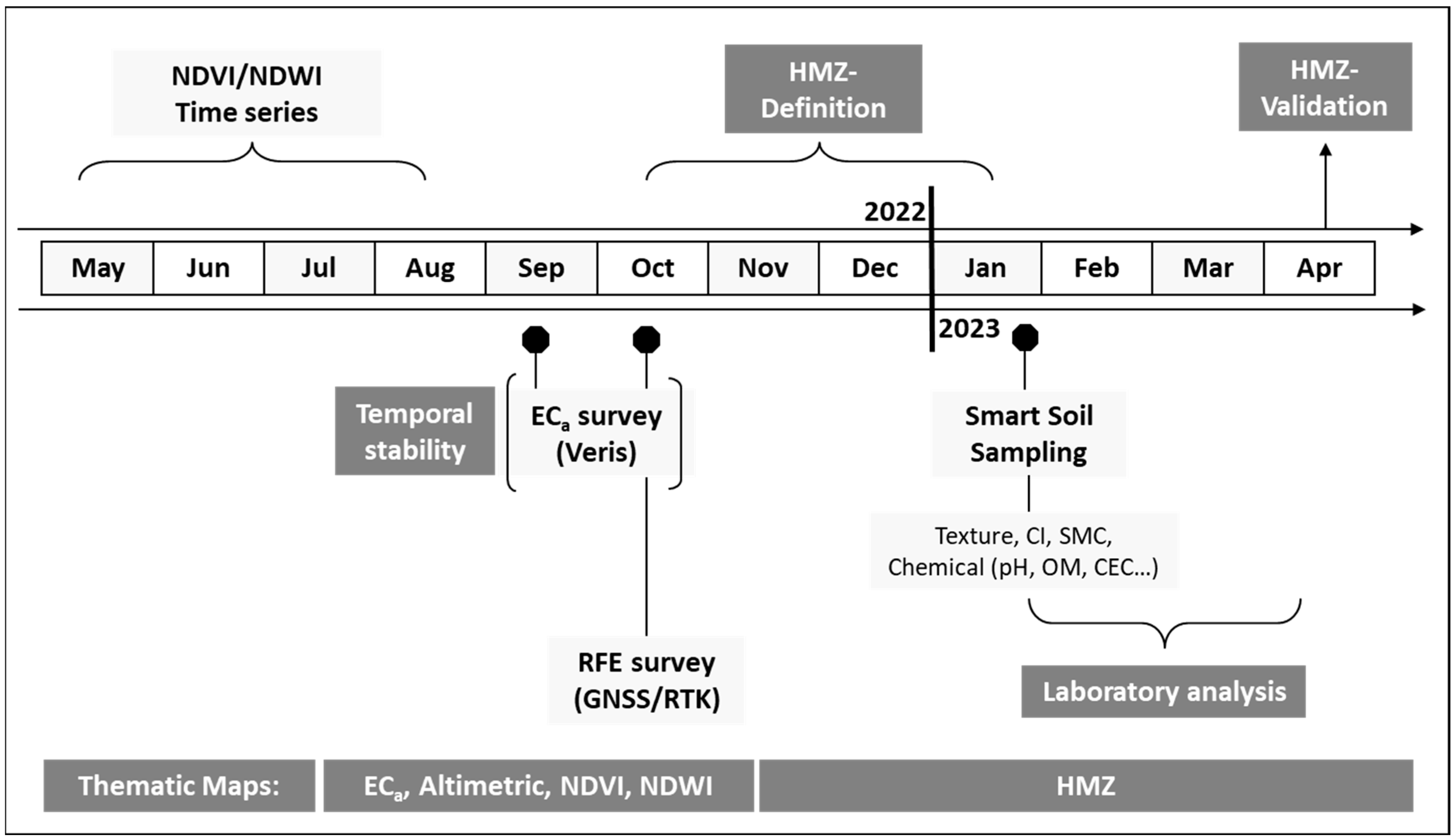
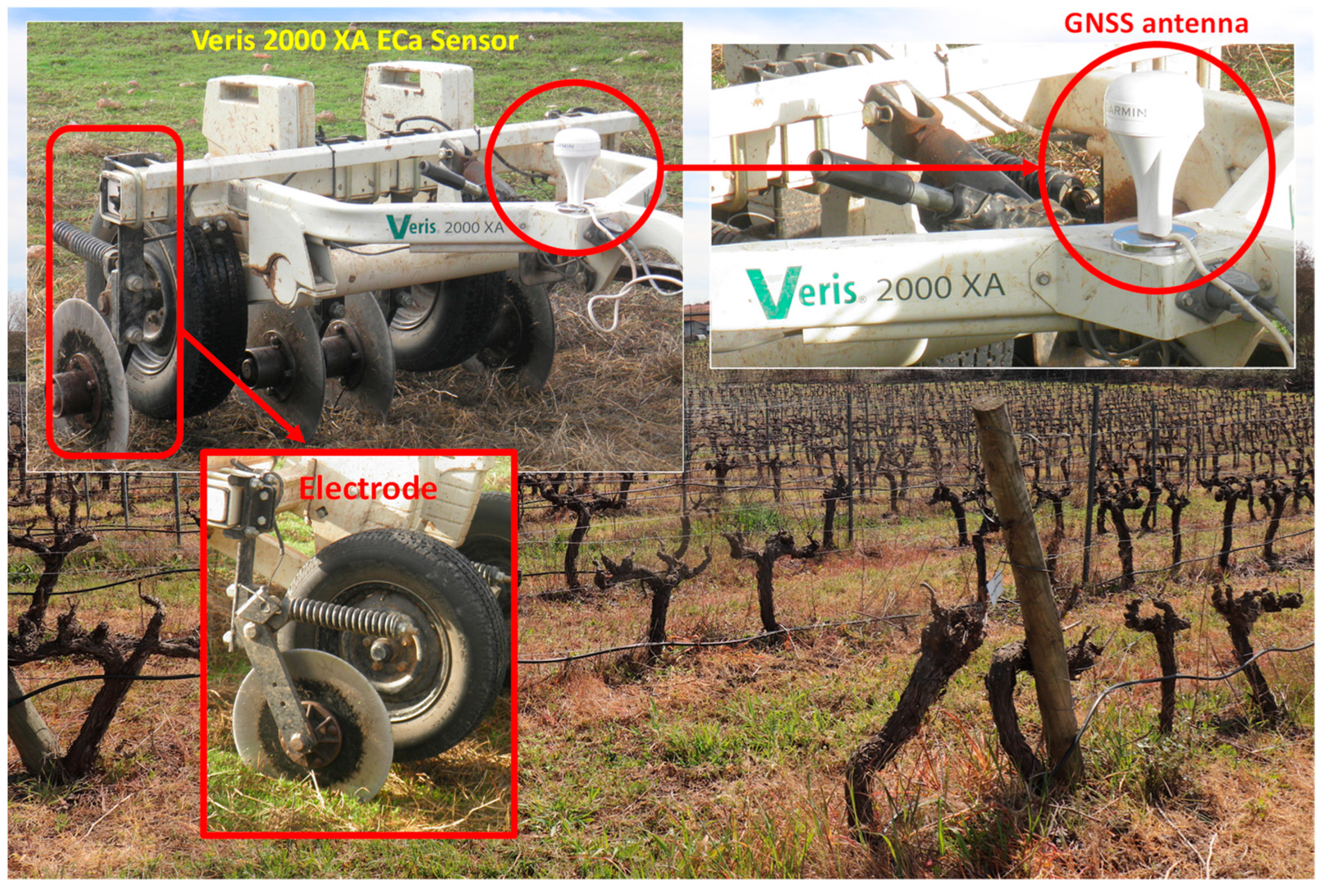
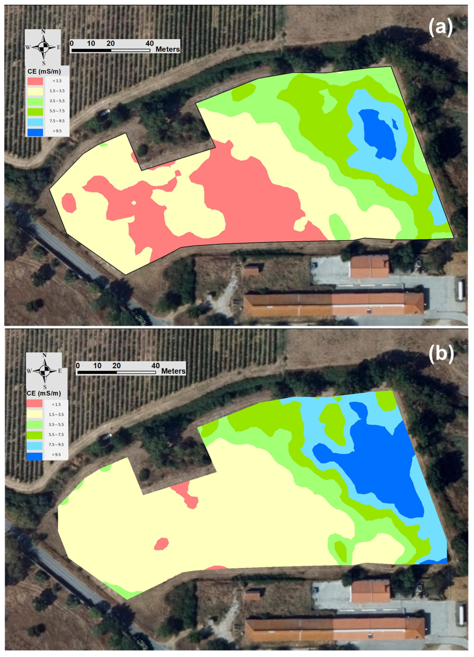
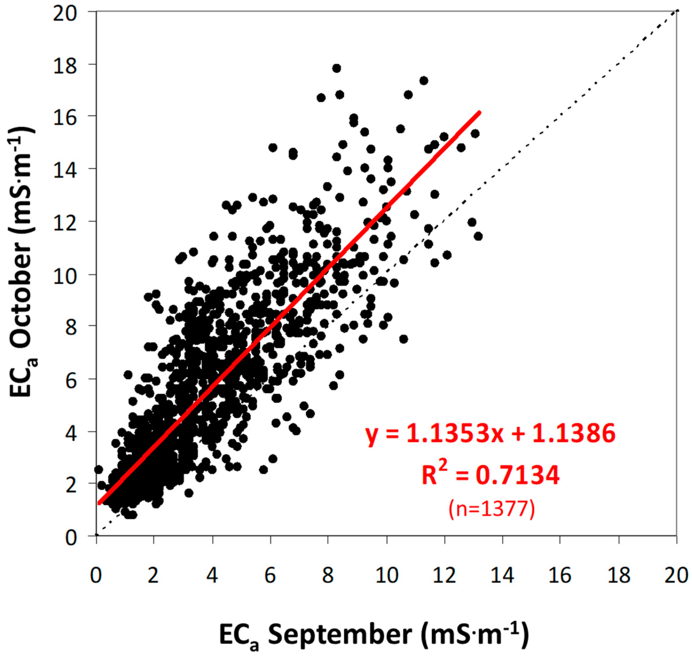
2.2. Soil Apparent Electrical Conductivity (EC_a) Surveys and Processing

The Veris 2000 XA contact-type sensor (Veris Technologies, Salina, KS, USA; Figure 5) equipped with a GNSS antenna was used to measure the soil EC_a of the experimental field on 29 September 2022 (only white grapes area) and on 24 October 2022 (whole field). This sensor is mounted on a chassis supported on two wheels and is formed by two pairs of coulter-electrodes (adjustable rotating discs): one pair injects a current into the soil (outermost discs), while the other pair (innermost discs) measures the voltage drop. The adjustment of the discs generated one set of topsoil data (from 0 to 0.30 m depths). The sensor was pulled by a four-wheel drive vehicle in the vineyard rows at an average speed of 5 km·h⁻¹ and was programmed to register the measurements each second.

On both dates (29 September and 24 October 2022), twenty random soil samples (0–0.30 m depth) were collected in the white grapes area to calculate the mean soil moisture content (SMC).

Estimating EC_a at unsampled locations was conducted with the ordinary point kriging algorithm, integrating the spatial correlation structure described with the variograms. The kriged maps showing the spatial distribution of EC_a in the experimental field were obtained from the estimated values. Finally, the kriged maps of EC_a were produced with the ArcMap module of the ArcGIS.

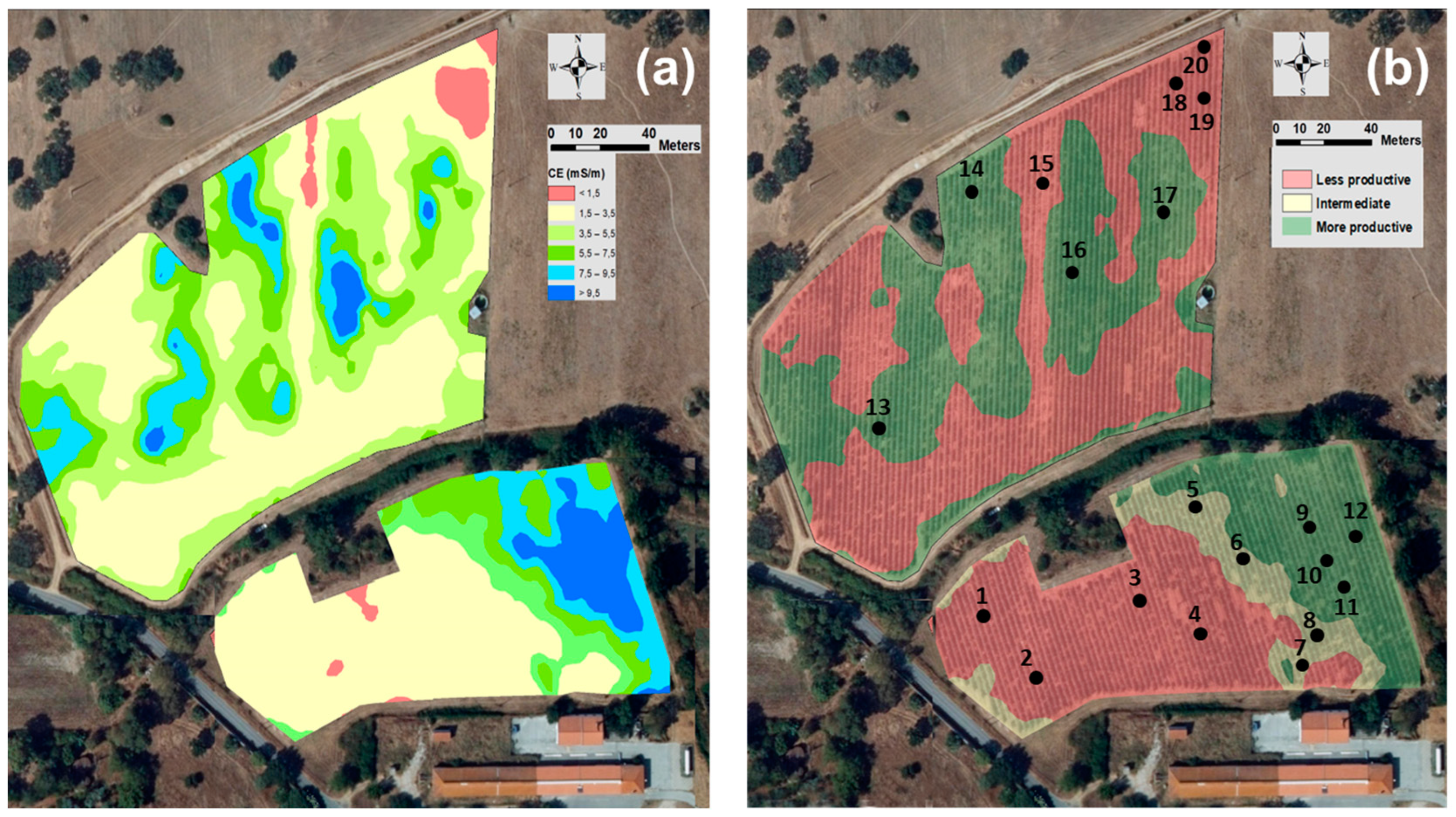
2.3. Definition of Management Zones (MZ)

The results of EC_a and altimetric surveys were used as input for the geostatistical analyses that allowed the definition of management zones (MZ). These homogeneous subfields were delineated using a fuzzy cluster algorithm [21]. The MZ Analyst (MZA) software (Microsoft Corp., Redmond, WA, USA) was utilized in this study. Fridgen et al. [22] described the procedures for delineating and evaluating the number of MZ used in this software. The fuzzy c-means, an unsupervised continuous classification procedure, which is implemented in the MZA program, was used to divide the fields into different cluster classes. The ISO Cluster approach in ArcGIS was used to perform the classification. This algorithm organizes the data in the input raster into a user-defined number of groups to produce signatures which are utilized to classify the data using the “Maximum Likelihood Classifier” (MLC) function. The fuzziness exponent was set at the conventional value of 1.3 and the “Mahalanobis” measure of similarity was selected since it is the most suitable for multivariate data classification [23]. From a practical perspective, three management zones with different productive potential (less, intermediate, and more potential) were considered in each vineyard area (white grapes, MZ: W−, W_int, and W+, respectively; and red grapes, MZ: R−, R_int, and R+, respectively). Both indices, the fuzziness performance index (FPI) and the normalized classification entropy (NCE) [22], confirmed that the number was adequate because their values were at minimum. FPI is a measure of the degree of membership sharing among classes: 0 indicates different classes with no membership sharing and 1 reflects a strong sharing of membership. NCE is an estimate of the amount of disorganization created by several classes: 0 indicates high organization and 1 represents a strong disorganization. When each index is at minimum, which indicates the least membership sharing (FPI) and greatest amount of organization (NCE) as a result of the clustering process, the optimum number of classes is achieved.

2.4. Validation of Management Zones (MZ)s

The validation of MZ was carried out by laboratory analysis of soil samples, measurements of soil compaction (CI) with an electronic cone penetrometer, and through indices (NDVI and NDWI) obtained by RS using Sentinel-2 satellite images.

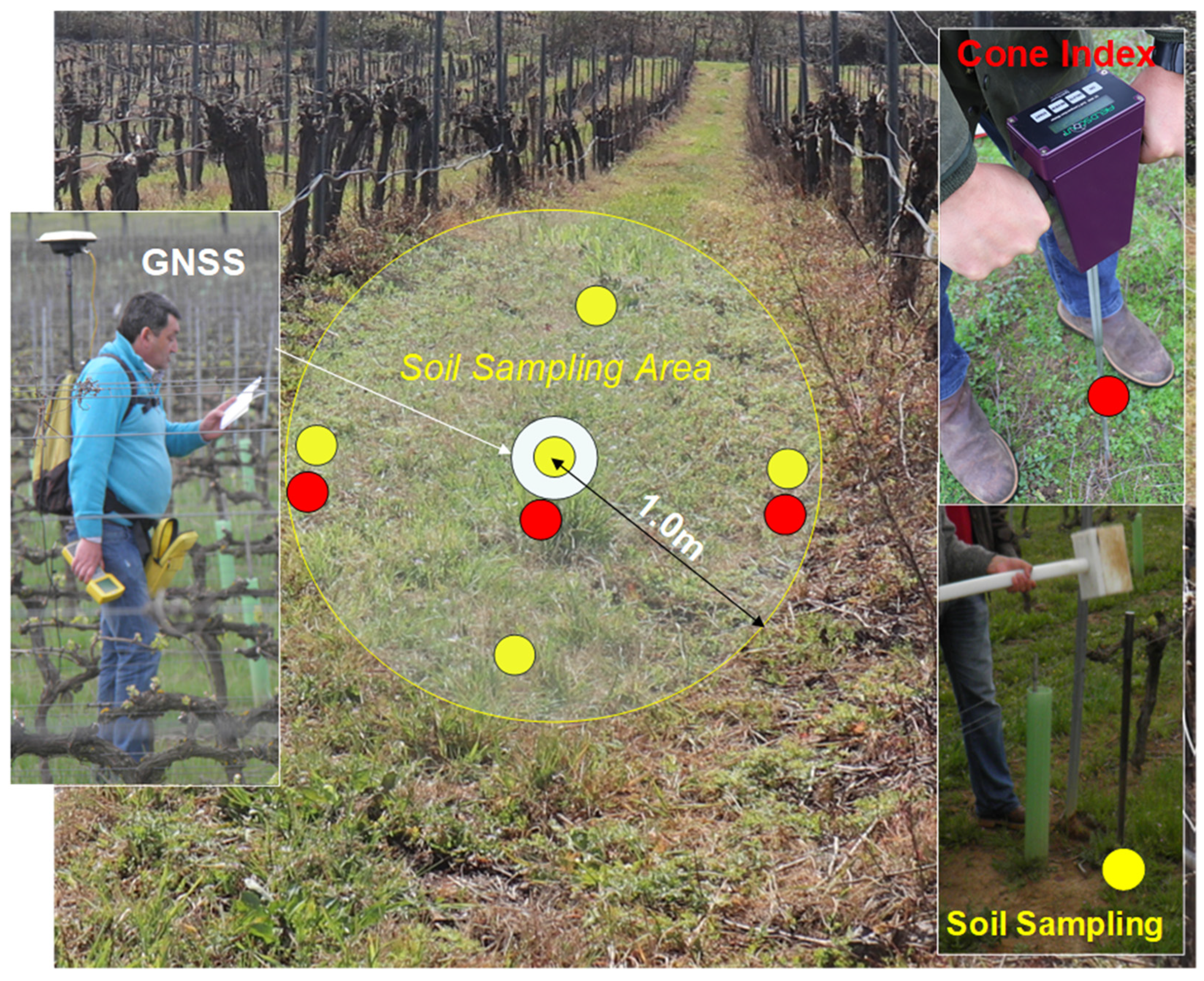
2.4.1. Soil Sampling Collection and Reference Analysis

After the definition of the MZs (with less, intermediate, and more productive potential), in the validation process (Figure 1), soil parameters (moisture content—SMC, CI, texture, pH, organic matter—OM, P₂O₅, K₂O, degree of base saturation–DBS, sum of the exchange bases—SEB, and cation exchange capacity—CEC), and crop vegetation indices (NDVI and NDWI) at sampling locations were employed to check their differences.

Four sampling areas were randomly GNSS georeferenced in each MZ and in each field (white and red grapes areas). The soil georeferenced samples were collected on 25 January 2023 using a gouge auger and a hammer, at a depth range of 0–0.30 m. Each composite sample was the result of five sub-samples collected within a radius of 1 m, one taken from the center of the sampling area, and the other four taken according to diagram presented in Figure 6. In the laboratory, the soil samples were weighed, dried at 105 °C until constant weight, and then weighed again to establish the SMC. Afterwards, the samples were processed for particle-size distribution (texture: sand, silt, and clay content) using a sedimentographer (Sedigraph 5100, manufactured by Micromeritics). The fine components of the soil (fraction with diameter < 2 mm) were subjected to chemical analyses using the following standard reference laboratory methods [24]: pH (in 1:2.5, soil: water suspension) was determined using the potentiometric method; organic matter (OM) was measured by combustion and CO₂ measurement, using an infrared detection cell; phosphorous (P₂O₅) and potassium (K₂O) were extracted by Egner–Riehm method, P₂O₅ was measured using colorimetric method, and K₂O was measured with a flame photometer; degree of base saturation (DBS), sum of the exchange bases (SEB; calcium—Ca²⁺, magnesium—Mg²⁺, sodium—Na⁺ and potassium—K⁺) and cation exchange capacity (CEC) were extracted with ammonium acetate.

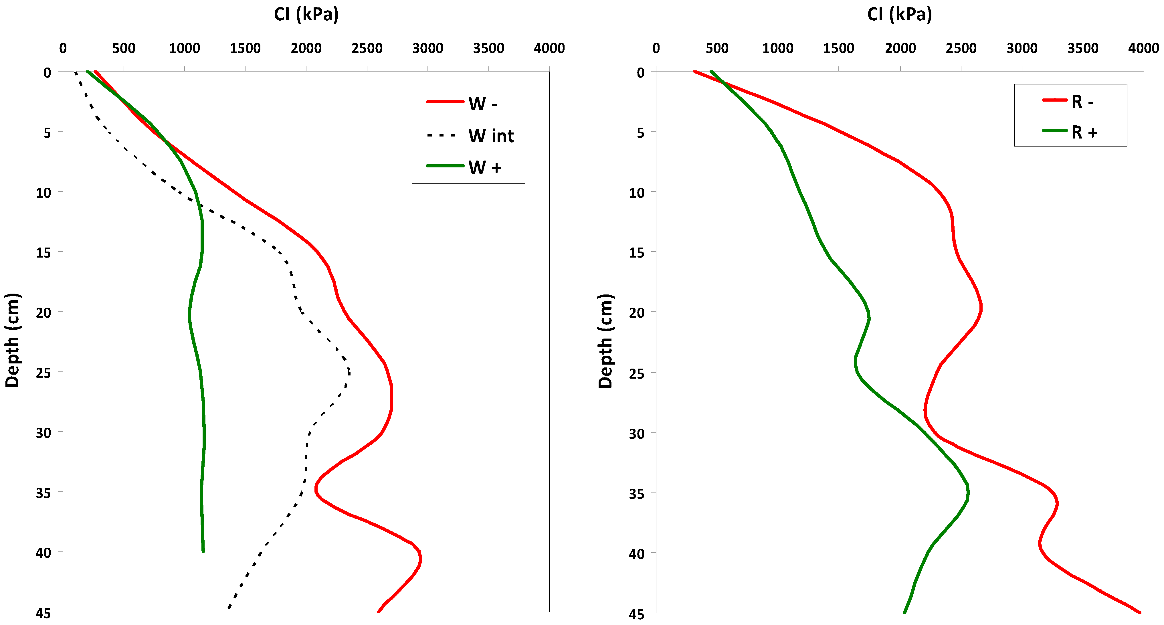
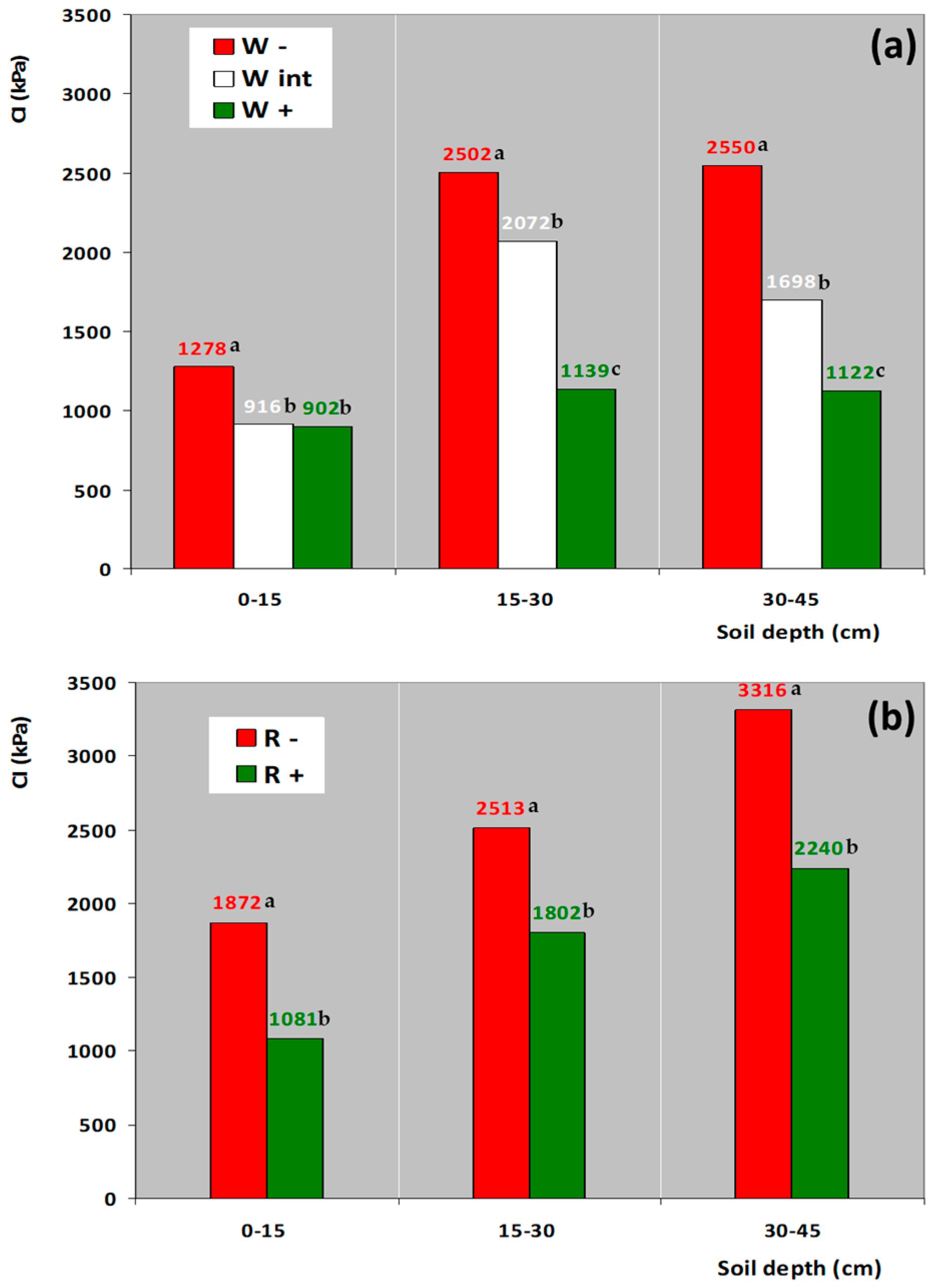
2.4.2. Cone Index (CI) Measurements

Simultaneously with the collection of soil samples, and as part of the validation process (Figure 1), the soil resistance to penetration (Cone Index, CI, in kPa) was measured with a manual electronic cone penetrometer “FieldScout SC 900” (Spectrum Technologies, Aurora, IL, USA). In each sampling point, three CI measurements were carried out between 0–45 cm depth, one in the central point of the sampling area, and one in each side next to each row of plants (Figure 6). To minimize possible errors resulting from the uncertainty of maintaining a constant penetration rate during the determination, measurements were always carried out by the same experienced operator. Readings for all treatments were taken on the same day to avoid soil moisture variability, which can affect the resistance measurements [13,14].

After the field measurements, the following data processing was implemented: (i) a preliminary analysis was conducted to remove outliers from the data set; (ii) the mean CI value of measurements of each sampling area of each MZ was calculated for each depth of determination (range of 2.5 cm); (iii) the graphic representation of mean CI as a function of soil depth (0–45 cm) for each MZ was generated; (iv) the mean CI values of measurements of each sampling area of each MZ was calculated for the following depth ranges: 0–15 cm, 15–30, and 30–45 cm.

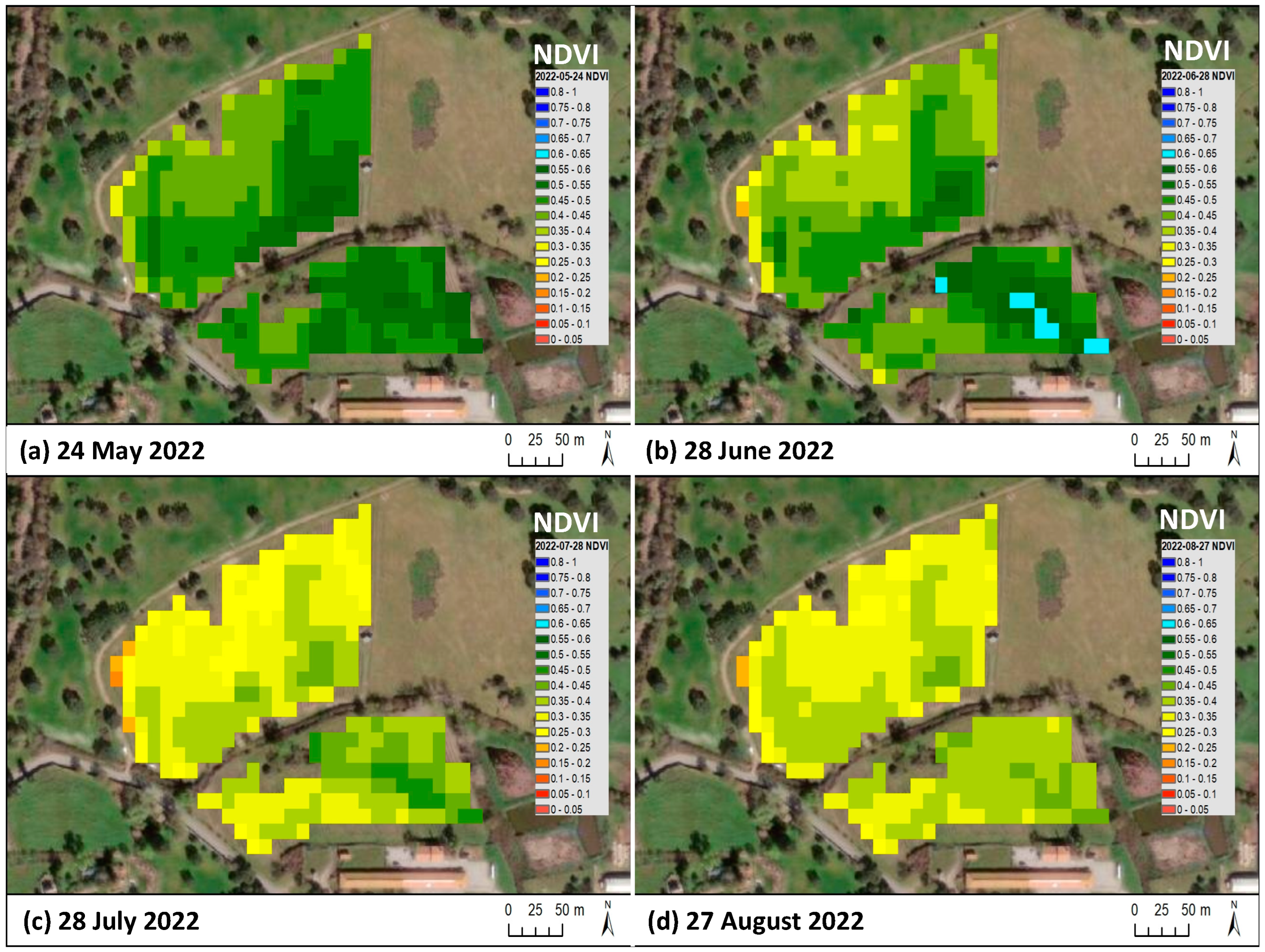
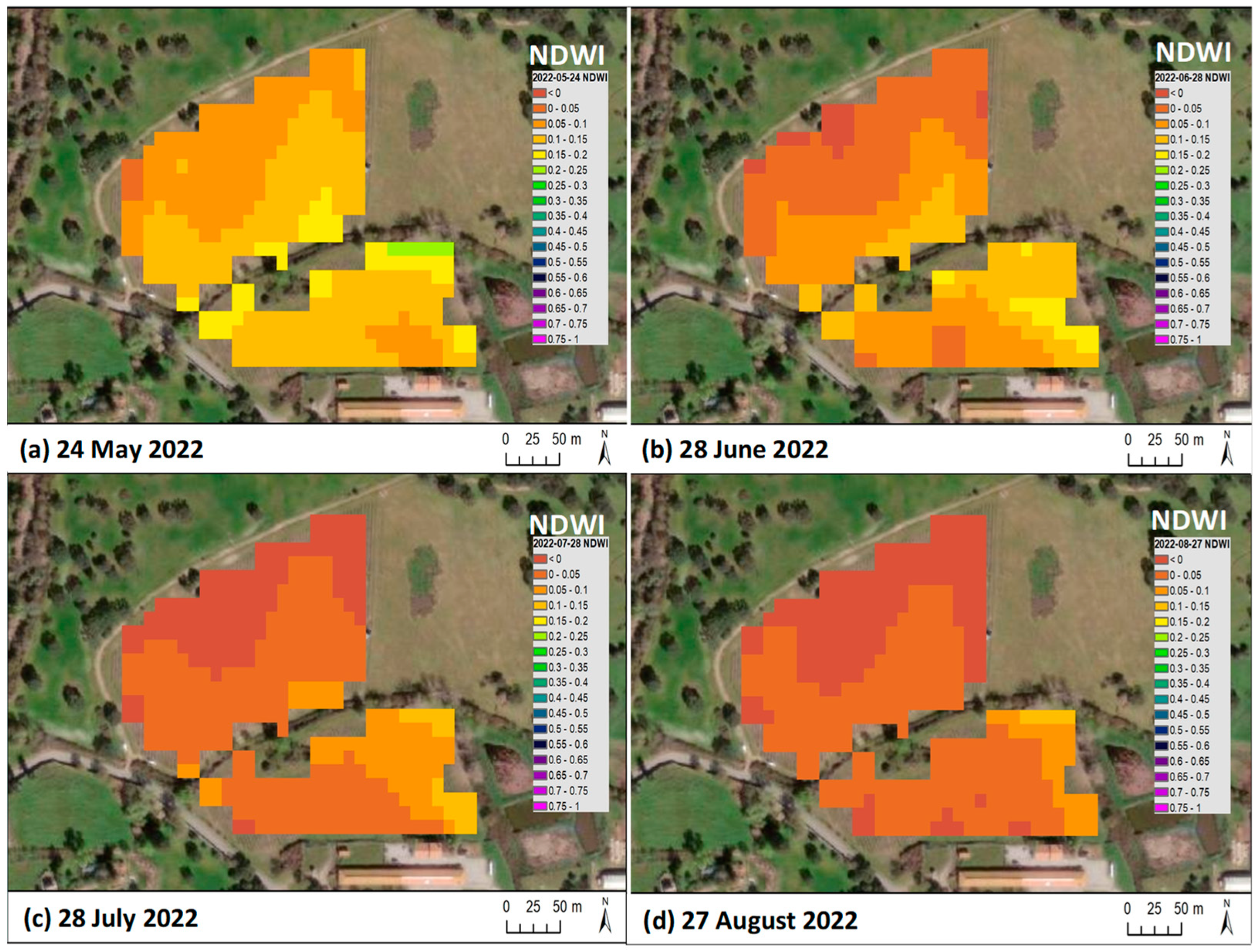
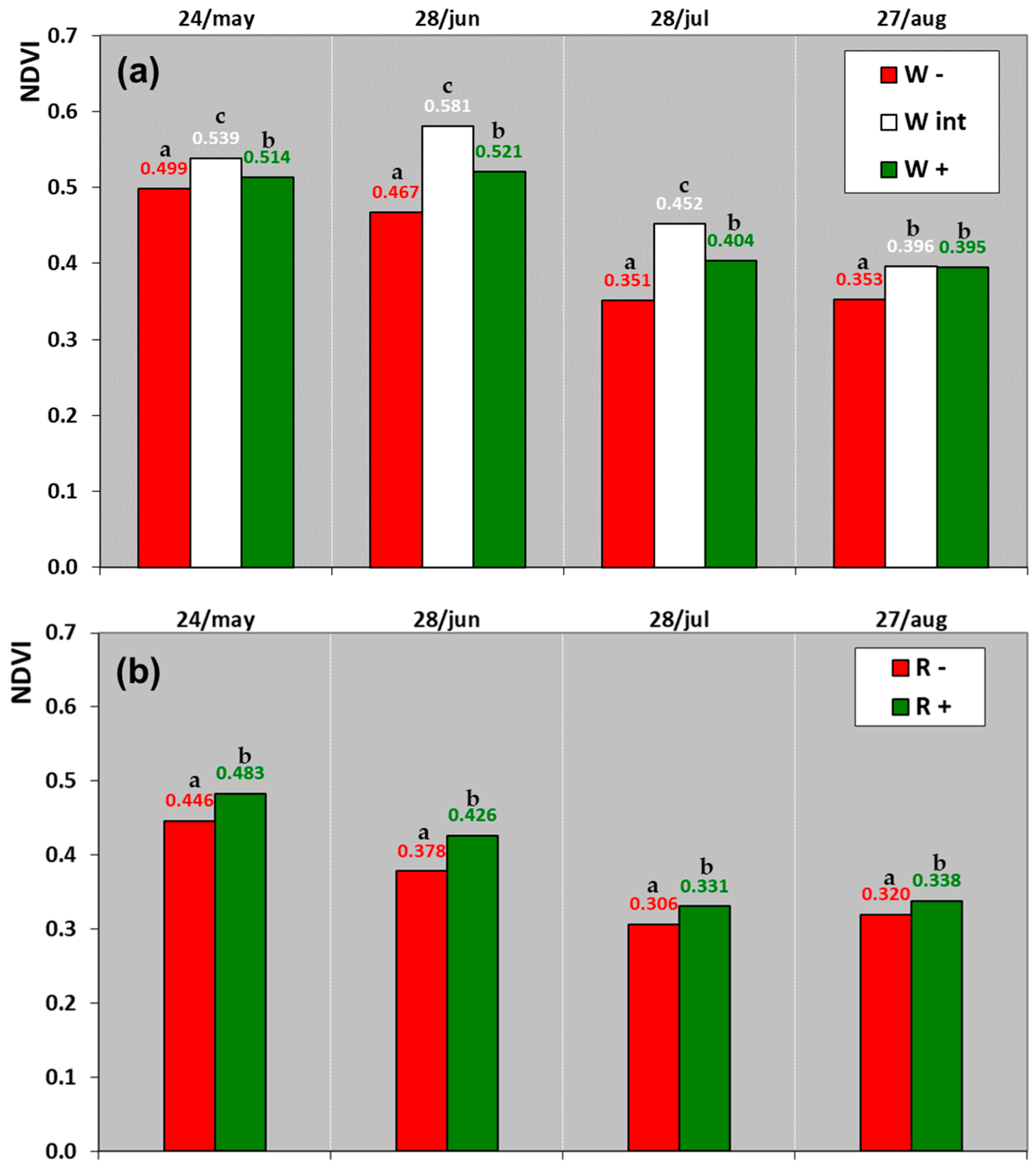
2.4.3. Multispectral Measurements by Remote Sensing

With the aim of monitoring the spatial variability of crop vegetative vigor, satellite images of the vegetative cycle of this vineyard in 2022 were retrieved (Figure 1). Sentinel-2 optical images (freely available from the European Space Agency, ESA), were used through the electronic platform “http://agromap.agroinsider360.com”. For this work, Sentinel-2 band 4 (B4; 10 m spatial resolution; 665 nm), band 8 (B8; 10 m spatial resolution; 842 nm), band 8A (B8A; 20 m spatial resolution; 865 nm), and band 11 (B11; 20 m spatial resolution; 1610 nm), atmospherically corrected imagery, were extracted from the Copernicus data hub and used to calculate NDVI (Equation (1)) and NDWI (Equation (2)). Images were processed with open-source ORG/GDAL Python libraries. These data were obtained for NDVI pixels (10 m resolution) and NDWI pixels (20 m resolution). A preliminary processing was carried out on these records to remove outliers due to the presence of clouds.

$$\mathrm{N}\mathrm{D}\mathrm{V}{\mathrm{I}}_{}=\frac{\mathrm{B}8-\mathrm{B}4}{\mathrm{B}8+\mathrm{B}4}$$

(1)

$$\mathrm{N}\mathrm{D}\mathrm{W}{\mathrm{I}}_{}=\frac{\mathrm{B}8\mathrm{A}-\mathrm{B}11}{\mathrm{B}8\mathrm{A}+\mathrm{B}11}$$

(2)

In the period of the vineyard’s greatest vegetative vigor (May–August) due to the favorable temperature and precipitation (Figure 4), four evaluation moments were considered, one at the end of each month (24 May, 28 June, 28 July, and 27 August), all from cloud-free satellite images. Figure 7 illustrates the vineyard in May 2022, where the contrast between the strong vigor of the canopy and the dry vegetation between the rows is visible.

In addition to the NDVI and NDWI maps for the referred dates, for the purposes of MZ validation, the average values of these indices in each MZ were calculated based in twenty sampling points used to soil collection.

2.5. Statistical Analysis of the Data

To assess the soil and crop spatial variability, descriptive statistical analysis (mean, standard variation, and range) was performed for the measured parameters.

The data of EC_a obtained by Veris sensor in September and in October were synchronized using the geographic co-ordinates of each point to evaluate the temporal stability of EC_a measurements. A combined data set was created in each date: each Veris data point obtained in September was combined with the nearest data point obtained in October based on GNSS co-ordinates. If a match in spatial co-ordinates was not found within a 2 m radius, that point was removed from the data set, a procedure like that used by Sudduth et al. [12]. A total of 1377 points were found to have common geographic co-ordinates in both surveys. These sets of data were subjected to linear correlation analysis, carried out in the IBM SPSS statistical package (version 24, IBM Corp, Armonk, NY, USA) to obtain the Pearson correlation coefficients (r) using the method of minimum squares (p < 0.05).

With the aim of evaluating if three MZ were significantly different, with a 95% significance level (p < 0.05), since the normality in the data cannot be assumed, the Kruskal–Wallis nonparametric test and the Dunn post hoc test were used. Thus, the differences in the mean values of both soil properties and crop indices were considered.

3. Results

3.1. From Spatial Variability to the Definition of Management Zones (MZ)

The soil variability associated with the topography (Figure 3) and consequent solar exposure and microclimate, the variety of vine cultivars (Figure 2), and the seasonality of temperature and precipitation (Figure 4) are factors that induce spatial variability. The vine responds accordingly, highlighting different physiological expressions [2]. The NDVI (Figure 8) and NDWI (Figure 9) maps referring to the previous year’s vegetative cycle (2022) show the evolution of the crop’s vegetative vigor and demonstrate this spatial variability.

This study aims to assess whether the expeditious monitoring of EC_a allows capturing, in a temporally stable way, the soil spatial variability. The maps of Figure 10 show important EC_a spatial variability in the white grapes field. Nevertheless, both maps indicate a stable pattern of EC_a, with a decreasing gradient from east to west (Figure 10a,b) and, simultaneously, a lower expression of low EC_a (<1.5 mS·m⁻¹) and a higher expression of high EC_a (>9.5 mS·m⁻¹) in the September map (Figure 10a), relative to the October map (Figure 10b). This temporal stability of EC_a pattern is evidenced by the significant correlation between the measurements of September and the measurements of October (Figure 11; R² = 0.7134), after synchronization of the geographical coordinates of the two surveys (n = 1377).

The EC_a spatial variability is common to the entire vineyard (

Table 1. Soil apparent electrical conductivity (EC_a) and soil moisture content (SMC) of vineyard in September and October 2022.

Parameter	Vineyard “W” (White Grapes)			Vineyard “R” (Red Grapes)
Date	Mean ± SD	CV (%)	Range	Mean ± SD	CV (%)	Range
ECa (mS·m−1) 29 September	3.6 ± 2.4	67.6	0.1–13.2	–	–	–
24 October	5.3 ± 3.4	64.9	0.8–17.8	4.6 ± 2.6	55.8	0.3–17.1
SMC (%) 29 September	14.6 ±4.1	28.1	10.3–19.5	–	–	–
24 October	17.7 ± 5.2	29.2	14.5–38.8	16.2 ± 1.3	8.1	14.0–18.7

SD—Standard deviation; CV—Coefficient of variation; EC_a—Soil apparent electrical conductivity; SMC—Soil moisture content.

), with a CV of around 65% in the white grapes field and 56% in the red grapes field. The SMC, however, shows less spatial variability, with a CV of around 29% in white grapes field and 8% in red grapes field (Table 1).

The transformation of the EC_a (based on the October measurement) and altimetric maps into a MZ map by applying a geostatistical algorithm is presented in Figure 12. Three MZ were defined in white grapes field (less, intermediate, and more productive potential) and, based on the lower EC_a spatial variability and, especially on the SMC, only two MZ were defined in red grapes field (less and more productive potential).

3.2. Validation of Management Zones (MZ)

The results of soil sampling (

Table 2. Characteristics of soil vineyard (0–0.30 m) in January 2023.

Soil Parameter	Vineyard “W” (White Grapes)			Vineyard “R” (Red Grapes)
(25 January 2023)	Mean ± SD	CV (%)	Range	Mean ± SD	CV (%)	Range
Clay (%)	14.9 ± 4.8	32.2	10.4–23.9	14.6 ± 6.0	41.2	7.4–26.5
Silt (%)	13.6 ± 3.0	22.4	10.6–19.0	11.3 ± 2.4	20.9	7.8–15.4
Sand (%)	71.5 ± 7.6	10.7	58.4–78.7	74.0 ± 7.9	10.7	61.1–84.9
SMC (%)	17.6± 4.4	25.0	11.2–27.5	14.6 ± 3.7	25.2	7.2–18.5
OM (%)	1.7 ± 0.5	30.7	1.0–2.5	1.0 ± 0.2	23.6	0.7–1.5
pH	6.5 ± 0.5	7.0	5.8–7.1	6.1 ± 0.5	8.8	5.6–7.0
P2O5 (mg.kg−1)	350.7 ± 209.1	59.6	101.4–722.6	28.9 ± 12.4	42.9	16.3–53.1
K2O (mg.kg−1)	118.7 ± 44.5	37.5	44.0–201.0	40.0 ± 24.7	61.8	10.0–78.2
DBS (%)	61.1 ± 33.6	55.0	13.5–121.9	61.4 ± 42.3	69.0	15.5–118.0
SEB (cmol.kg−1)	8.2 ± 5.4	65.0	3.3–18.0	8.7 ± 7.1	81.1	2.0–19.7
CEC (cmol.kg−1)	14.9 ± 5.9	39.5	8.2–28.0	18.2 ± 11.1	61.0	8.3–41.8

SD—Standard deviation; CV—Coefficient of variation; SMC—Soil moisture content; OM—Organic matter; P₂O₅—Assimilable phosphorous; K₂O—Assimilable potassium; DBS—Degree of base saturation; SEB—Sum of the exchange bases; CEC—Cation exchange capacity (CEC).

) show that it is a coarse to medium textured soil (clay content of about 15%; textural classification between sandy loam and sandy clay loam) [19], with low OM content (especially in red grapes field, with 1%), pH close to neutral, with strong contrast between the two subfields in terms of phosphorus and potassium availability (extremely high in white grapes field and low in red grapes field). The spatial variability is very pronounced, with CV greater that 20–30% in practically all soil evaluated parameters, except for pH (CV of 7–9%) and sand content (CV of 11%).

The validation of the MZ defined in each field (white and red grapes areas) based on the differences in the mean values of soil properties (

Table 3. Validation of management zones (MZ): mean values of each soil property for MZ (less productive zone, “Less”; intermediate zone, “Inter.”; and more productive zone, “More”).

MZ	Clay (%)	Silt (%)	Sand (%)	SMC (%)	OM (%)	pH	P2O5 (mg·kg−1)	K2O (mg·kg−1)	DBS (%)	SEB (cmol·kg−1)	CEC (cmol·kg−1)
“White”
Less	12.2 a	11.3 a	76.5 a	14.7 a	1.2 a	6.0 a	204.7 a	113.8 a	34.0 a	3.7 a	14.2 a
Inter.	11.7 a	12.2 a	76.2 a	18.2 b	1.6 b	6.6 b	341.2 b	134.5 b	46.4 b	5.9 b	16.7 b
More	20.9 b	17.4 b	61.8 b	19.8 c	2.2 c	7.0 c	506.1 c	107.8 a	103.0 c	15.1 c	18.0 c
“Red”
Less	10.8 a	9.6 a	79.6 a	12.1 a	0.9 a	5.7 a	38.0 a	47.8 a	23.2 a	2.5 a	15.1 a
More	18.5 b	13.1 b	68.5 b	17.0 b	1.2 b	6.6 b	19.9 b	33.0 b	99.5 b	15.0 b	21.3 b

MZ—Management zones; SMC—Soil moisture content; OM—Organic matter; P₂O_5—Assimilable phosphorous; K₂O—Assimilable potassium; DBS—Degree of base saturation; SEB—Sum of the exchange bases; CEC—Cation exchange capacity (CEC); Different letters indicate significant differences (p < 0.05) according to the Dunn test.

) confirmed significantly higher values of clay, silt, SMC, OM, pH, DBS, SEB, and CEC and significantly lower values of sand in MZ with greater productive potential (“More”).

In terms of CI (

Table 4. Cone index (CI) of soil vineyard in three depths (0–15, 15–30, and 30–45 cm) in January 2023.

CI (kPa)	Vineyard “W” (White Grapes)		Vineyard “R” (Red Grapes)
MZ—Depth (cm)	Mean ± SD	Range	Mean ± SD	Range
Less potential
0–15	1278 ± 632	440–2091	1872 ± 511	1169–2467
15–30	2502 ± 184	2256–2673	2513 ± 183	2283–2730
30–45	2550 ± 308	2078–2928	3316 ± 340	2973–3967
Intermediate
0–15	916 ± 639	172–1768	–	–
15–30	2072 ± 151	1941–2355	–	–
30–45	1698 ± 338	1265–2070	–	–
More potential
0–15	902 ± 281	405–1143	1081 ± 274	677–1393
15–30	1139 ± 98	1030–1298	1802 ± 224	1587–2199
30–45	1122 ± 92	970–1220	2240 ± 302	1759–2557

SD—Standard deviation; CI—Cone index.

; Figure 13; Figure 14), the results show a tendency for (i) higher values in the red grapes field than in the white grapes field; (ii) higher values in MZ with lower productive potential; (iii) higher values as depth increases; (iv) higher CV (25–70%) in the topsoil layer (0–15 cm). The graphical representation of the average CI in the topsoil layer (0–30 cm), in each MZ, as a function of mean SMC (Figure 15) confirms the inverse relationship between CI and SMC.

In terms of validating the MZ based on the vineyard vegetative vigor measured by RS indices, NDVI (

Table 5. Normalized difference vegetation index (NDVI) of vineyard (white and red grapes fields) in each MZ, on four dates in 2022 (24 May, 28 June, 28 July, and 27 August).

NDVI	Vineyard “W” (White Grapes)		Vineyard “R” (Red Grapes)
MZ—Date (2022)	Mean ± SD	Range	Mean ± SD	Range
Less potential
24 May	0.499 ± 0.030	0.469–0.538	0.446 ± 0.019	0.432–0.460
28 June	0.467 ± 0.022	0.447–0.498	0.378 ± 0.037	0.352–0.404
28 July	0.351 ± 0.015	0.343–0.374	0.306 ± 0.029	0.286–0.326
27 August	0.353 ± 0.003	0.350–0.357	0.320 ± 0.027	0.300–0.339
Intermediate
24 May	0.539 ± 0.018	0.527–0.559	–	–
28 June	0.581 ± 0.047	0.527–0.613	–	–
28 July	0.452 ± 0.046	0.400–0.485	–	–
27 August	0.396 ± 0.010	0.384–0.402	–	–
More potential
24 May	0.514 ± 0.022	0.488–0.526	0.483 ± 0.031	0.450–0.525
28 June	0.521 ± 0.004	0.519–0.526	0.426 ± 0.042	0.381–0.474
28 July	0.404 ± 0.003	0.400–0.405	0.331 ± 0.026	0.301–0.364
27 August	0.395 ± 0.010	0.384–0.401	0.338 ± 0.023	0.311–0.362

SD—Standard deviation; NDVI—Normalized difference vegetation index.

; Figure 16) and NDWI (

Table 6. Normalized difference water index (NDWI) of vineyard (white and red grapes fields) in each MZ, on four dates in 2022 (24 May, 28 June, 28 July, and 27 August).

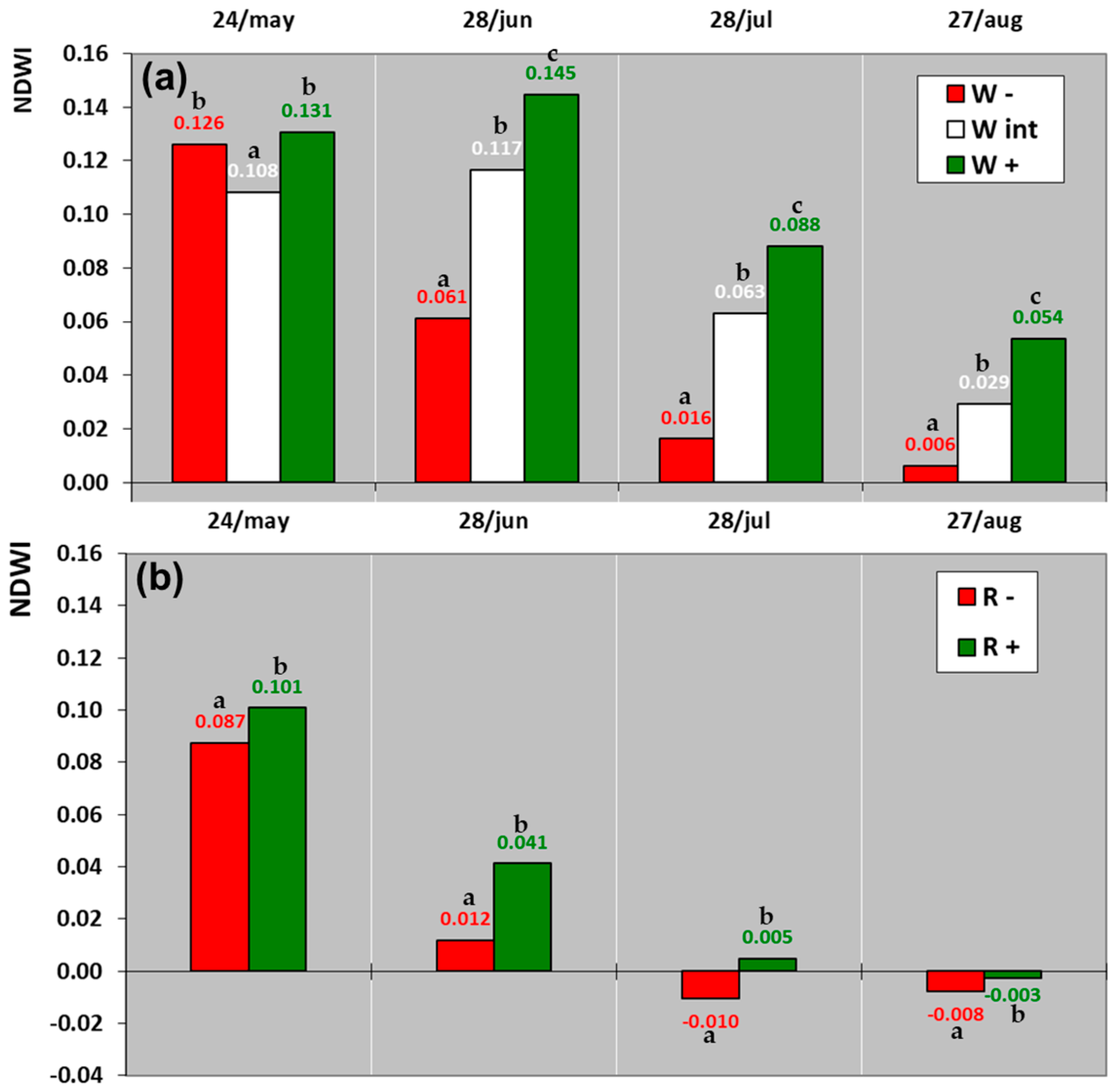
NDWI	Vineyard “W” (White Grapes)		Vineyard “R” (Red Grapes)
MZ—Date (2022)	Mean ± SD	Range	Mean ± SD	Range
Less potential
24 May	0.126 ± 0.013	0.113–0.139	0.087 ± 0.013	0.078–0.097
28 June	0.061 ± 0.018	0.038–0.082	0.012 ± 0.003	0.010–0.014
28 July	0.016 ± 0.007	0.006–0.022	−0.010 ± 0.002	−0.012–(−0.009)
27 August	0.006 ± 0.005	0.000–0.013	−0.008 ± 0.006	−0.012–(−0.003)
Intermediate
24 May	0.108 ± 0.015	0.095–0.126	–	–
28 June	0.117 ± 0.041	0.059–0.149	–	–
28 July	0.063 ± 0.031	0.022–0.097	–	–
27 August	0.029 ± 0.021	−0.002–0.041	–	–
More potential
24 May	0.131 ± 0.008	0.121–0.137	0.101 ± 0.019	0.073–0.115
28 June	0.145 ± 0.014	0.137–0.165	0.041 ± 0.028	0.006–0.065
28 July	0.088 ± 0.001	0.087–0.089	0.005 ± 0.017	−0.017–0.020
27 August	0.054 ± 0.003	0.051–0.056	−0.003 ± 0.016	−0.020–0.011

SD—Standard deviation; NDWI—Normalized difference water index.

; Figure 17) in the vegetative cycle of 2022, the results show (i) a gradual decrease in NDVI and NDWI as the vegetative cycle progresses; (ii) higher values in the white grapes field than in the red grapes field; (iii) higher values in MZ with more productive potential.

4. Discussion

The interest in PV has been highlighted in several reviews published in recent years [2,10,25,26]. Research of PV have focused on four main areas: (i) evaluation of spatial variability; (ii) delimitation of MZ; (iii) development of variable rate technologies (VRT); and (iv) implementation of site-specific vineyard management [2]. This study focuses on the first two areas: to assess the soil spatial variability in a vineyard, and to define and validate MZ.

4.1. Spatial Variability

Spatial variability is the starting point that justifies the implementation of the PA concept [2]. The MZ represent the link between spatial variability and potential differentiated management [4,7].

Mobile soil EC_a measurements constitute one of the most efficient ways to quickly map soil spatial variability [7,17]. According to Ammoniaci et al. [2] and Rodriguez-Pérez et al. [27], EC_a could save time and resources during the planning and establishment of new vineyards and, also, during monitoring and management of established vineyards. The CV of EC_a obtained in this study (about 60%) classifies this parameter as having high spatial variability [5] and, therefore, is a potential indicator of the soil characteristics, which suggest the convenience of defining different MZ [7]. In this study, terrain elevation was also used in MZ delineation due to its impact on water flow and accumulation, as well as redistribution of soil mineral particles and OM, and, therefore, on crop growth and development [4,6]. Other works have sought to complement the EC_a information with other parameters, namely crop vegetative vigor. Esteves et al. [9], for example, associated the NDVI measurement, obtained from the Sentinel-2 satellite images, with EC_a to define three zones of differentiated vine management. Serrano et al. [28] also associated the EC_a with NDVI and NDWI to define three MZ, but in pasture management.

Although several factors may contribute to the variability of vineyard development (soil, topography, grape varieties, etc.) [3], the NDVI (Table 5) showed a relatively low CV (<10%) on all assessment dates, which may reflect, on the one hand, the uniform cultural operations carried out throughout the vineyard (e.g., pruning, shoot and grape thinning and, especially, canopy management) [18], but mainly the sampling procedure used in the MZ validation, based only on 20 sampling points and not on the whole vineyard area (contrary to what happened in the EC_a measurement, carried out practically continuously). In contrast, the NDVI and NDWI maps (Figure 8; Figure 9, respectively), represent the entire area of the vineyard and attest to the expression of the variability identified by the EC_a measurement.

In addition to spatial variability, another important characteristic that should be assessed in a PV process is the within-field temporal stability of spatial patterns [29]. Measuring EC_a is frequently conducted to reveal this spatial soil heterogeneity. Various studies have demonstrated the possibilities for significant changes in the measured quantities over time with relatively stable spatial structure representations [30]. One of the great advantages of EC_a measurement is its temporal stability, maintaining the spatial pattern over time, so it only needs to be measured once in the medium term [31]. In this study, the EC_a surveys of September and October led to similar EC_a maps (Figure 10), with a strong R² (0.7134; Figure 11). The positive effect of SMC (higher in October that in September, which reflects an accumulated precipitation of 75 mm in the week preceding the measurement in October, while in the week preceding the measurement in September the accumulated precipitation was only 18 mm) in EC_a is reported in several works [2,26]. This temporal stability allows decision making in post-processing, which avoids the technological complexity of real-time variable application systems.

4.2. Validation of Management Zones (MZ)

The EC_a can help to guide the sampling for the purpose of characterizing the spatial variability [11]. The validation of the defined MZ was carried out by smart sampling of (i) soil parameters (texture, SMC, pH, OM, phosphorous, potassium, DBS, SEB, CEC, and CI); and (ii) normalized indices (NDVI and NDWI) obtained by RS.

Areas with higher EC_a led to MZ with more productive potential, and vice-versa (Figure 12). The validation showed that the zones with more productive potential present a soil profile (0–30 cm depth) with higher clay, moisture, OM, pH, DBS, SEB, and CEC contents, and lower sand content and CI values (this last parameter in all the depth classes that were considered: 0–15, 15–30, and 30–45 cm), which is reflected in higher vine vegetative vigor (higher NDVI and NDWI). The relationship between EC_a and soil texture has been documented in several studies [2,7,9,11,17,32], positively correlated with the finer texture component, clay, and negatively correlated with the coarser textures such as coarse and fine sands [7,17,25], even leading to the indication of specific reference values of EC_a for certain soil characteristics (rocky substrate, sand, clay, water, etc.) [2]. Mean EC_a of 3–6 mS·m⁻¹ (Table 1) classify the soil of this vineyard as coarse-textured and dryland soils [14], typical of this region of South of Portugal. The relationship between EC_a and others soil physical and chemical properties, namely OM content [2], SMC [17,27,29], CEC, pH, exchangeable magnesium, and other soil nutrients [9], has been demonstrated across a wide range of soils [12]. In arid or semiarid regions, for example, moisture availability is the primary factor that controls land productivity; therefore, SMC should be considered as one of the most important factors to delimit management zones, which is very dependent on the topography of the field [33]. In this study, however, the main macronutrients phosphorus and potassium (P₂O₅ and K₂O, respectively) did not follow the trend defined by the MZ in white grapes area, with mean contents very high in intermediate MZ (Table 3). This result makes it difficult to transpose these MZ maps to fertilization prescription maps. Since these abnormally high values of P and K occur only in the white grapes area (Table 2), where the OM values are also much higher (mean of 1.7% versus 1.0% in red grapes area), the proximity of a pigsty (upstream of the white grape vineyard and of a water flow line) could be the origin of this unexpected pattern, which may have led the geostatistical algorithm to set an intermediate MZ in this field. In this case, the intermediate MZ can be an indicator of this external effect (drainage of effluents from intensive livestock production) on topsoil spatial variability. If fertilization was based on a composite sample of the entire vineyard area of 3.3 ha, as is common practice in traditional agriculture in the region, the average values of P and K would be adequate (more than 100 mg·kg⁻¹) and therefore would not justify fertilization, however, spatial analysis shows, for example, that the red grapes area has low P and K values (around 30–40 mg·kg⁻¹), which requires P and K fertilization.

The inverse correlation between EC_a and soil compaction (zones with more productive potential present systematically lower CI values) is in line with several other works [13,14,27,34,35], some of them even suggesting the potential of EC_a as a rapid alternative for assessing soil compaction [34,35].

Relatively to validation of MZ through of RS indices, the results of Ferrer et al. [3] suggest that NDVI could be a useful tool for defining and categorizing zones (high, medium, and low) within the vineyards in order to establish site-specific management practices according to the grapevine needs. Tardaguilla et al. [10], in a review paper about the use of smart technologies in viticulture, reinforces the relevance of vine vigor maps from previous years in designing site-specific management strategies for the upcoming year. Comparetti and Silva [16], on the other hand, demonstrated the usefulness of NDVI and NDWI obtained from the Sentinel-2 satellite images to identify the same three levels of vegetative vigor (high, medium, and low) and support decision making for vintage segmentation, which makes it possible process different quality grapes to produce different wines, differentiating the grapes on the basis of their potentiality and typicality, highlighting the “terroir effect” over the years [2]. Comparetti and Silva [16] also foresee the use of NDVI and NDWI in variable rate fertilizer application, however, point out the challenge to be overcome in PV in terms of establishing correlations between plant vegetative vigor, crop yield, wine quality, and soil parameters in order to produce spatially variable input application maps that can increase crop yields. The successful results documented by Hubbard et al. [17] in a vineyard, using pixel-by-pixel as well as block-by-block comparisons lay the groundwork for future research directions; for example, the significant correlation between soil texture, EC_a, and NDVI suggest that vegetation properties during the growing season could be estimated, and possibly predicted, through soil texture or EC_a information.

4.3. Study Limitations and Perspectives

Given that this is an exploratory study, carried out in a relatively restricted area of vineyard (3.3 ha), under specific soil and climatic conditions, further studies, in different soil types and different regions should be conducted.

An important note should be considered: several studies showed a direct correlation between NDVI and crop yield components, suggesting that the zones with the highest vigor are also the highest yielding. However, in the vineyard the issue is complex, with zones of low vigor (NDVI) tending to produce higher quality wine in some instances [36]. Since the main aim of modern oenology is to produce wines of recognized quality and typically, which can then be differentiated in the market, it is essential to consider that the potential quality of wine is established in the vineyard [5]. Therefore, it will be interesting in the next campaign to evaluate the impact of this topsoil spatial variability on productivity (yield maps) and, especially, on grape quality and, consequently, on wine quality, using a segmented harvest to clarify the practical impact and the agronomic significance of this MZ delineation.

It is also fundamental to develop algorithms to evaluate the agronomic significance of this classification (MZ) and establish more general methods of mapping and quantifying variable input prescriptions based in EC_a.

The closing of the PA cycle by agricultural machinery (namely fertilizer distributors or sprayers), based on prescription maps (built from MZ), or other means, provides a rigorous variable rate application [37]. Despite the existence of this technologies to improve and maximize efficiency of inputs and profitability of individual fields [38], the scattered and interlaced MZ delineation can be challenging for the farmer, and in some cases, it might be advisable to unify the MZ to larger working units in order to simplify the operationalization of the process.

5. Conclusions

The results of this study showed that the use of fast and easy tools for measuring and mapping EC_a and altimetry allows capturing, in a temporally stable way, the spatial variability of physical (texture, compaction, moisture) and chemical (pH, OM, degree of base saturation, exchange bases, and cation exchange capacity) topsoil (0–30 cm) characteristics, leading to the definition and validation of zones (MZ) of high and low productive potential. These MZ may be relevant when designing new vineyards or replanting existing vineyards, e.g., for the selection of the most adapted cultivars, or for field orientation (sun exposure, drainage, etc.) for a given “terroir”. This approach can also be useful for a more-informed decision-making process for site-specific management of inputs and guide viticultural practices. The ability to map the soil spatial variability allows grape growers to move from a random soil sampling to an optimized methodology based on MZ (smart soil sampling).

It will be important to validate these results in other conditions, with different soil types or in different regions, extending the database and so, improve the process for prescribing spatially differentiated inputs.

References

- Casson, A.; Ortuani, B.; Giovenzana, V.; Brancadoro, L.; Corsi, S.; Gharsallah, O.; Guidetti, R.; Facchi, A. A multidisciplinary approach to assess environmental and economic impact of conventional and innovative vineyards management systems in Northern Italy. Sci. Total Environ. 2022, 838, 156181. [Google Scholar] [CrossRef]
- Ammoniaci, M.; Kartsiotis, S.-P.; Perria, R.; Storchi, P. State of the art of monitoring technologies and data processing for Precision Viticulture. Agriculture 2021, 11, 201. [Google Scholar] [CrossRef]
- Ferrer, M.; Echeverría, G.; Pereyra, G.; Gonzalez-Neves, G.; Pan, D.; Mirás-Avalos, J.M. Mapping vineyard vigor using airborne remote sensing: Relations with yield, berry composition and sanitary status under humid climate conditions. Prec. Agric. 2020, 21, 178–197. [Google Scholar] [CrossRef]
- Córdoba, M.; Bruno, C.; Costa, J.; Balzarini, M. Subfield management class delineation using cluster analysis from spatial principal components of soil variables. Comput. Electron. Agric. 2013, 97, 6–14. [Google Scholar] [CrossRef]
- Unamunzaga, O.; Besga, G.; Castellón, A.; Usón, M.A.; Chéry, P.; Gallejones, P.; Aizpurua, A. Spatial and vertical analysis of soil properties in a Mediterranean vineyard soil. Soil Use Manag. 2014, 30, 285–296. [Google Scholar] [CrossRef]
- Verdugo-Vásquez, N.; Acevedo-Opazo, C.; Valdés-Gómez, H.; Pañitrur-De la Fuente, C.; Ingram, B.; García de Cortázar-Atauri, I.; Tisseyre, B. Identification of main factors affecting the within-field spatial variability of grapevine phenology and total soluble solids accumulation: Towards the vineyard zoning using auxiliary information. Precis. Agric. 2022, 23, 253–277. [Google Scholar] [CrossRef]
- Moral, F.; Terrón, J.; Silva, J.M. Delineation of management zones using mobile measurements of soil apparent electrical conductivity and multivariate geostatistical techniques. Soil Tillage Res. 2010, 106, 335–343. [Google Scholar] [CrossRef]
- Sams, B.; Bramley, R.G.V.; Sanchez, L.; Dokoozlian, N.; Ford, C.; Pagay, V. Remote sensing, yield, physical characteristics, and fruit composition variability in Cabernet Sauvignon vineyards. Am. J. Enol. Vitic. 2022, 73, 93–105. [Google Scholar] [CrossRef]
- Esteves, C.; Fangueiro, D.; Braga, R.P.; Martins, M.; Botelho, M.; Ribeiro, H. Assessing the contribution of ECa and NDVI in the delineation of management zones in a vineyard. Agronomy 2022, 12, 1331. [Google Scholar] [CrossRef]
- Tardaguila, J.; Stoll, M.; Gutiérrez, S.; Proffitt, T.; Diago, M.P. Smart applications and digital technologies in viticulture: A review. Smart Agric. Technol. 2021, 1, 100005. [Google Scholar] [CrossRef]
- Bottega, E.L.; Marin, C.K.; Oliveira, Z.B.d.; Lamb, C.D.C.; Amado, T.J.C. Soil density characterization in management zones based on apparent soil electrical conductivity in two field systems: Rainfeed and center-pivot irrigation. AgriEngineering 2023, 5, 460–472. [Google Scholar] [CrossRef]
- Sudduth, K.A.; Kitchen, N.R.; Bollero, G.A.; Bullock, D.G.; Wiebold, W.J. Comparison of electromagnetic induction and direct sensing of soil electrical conductivity. Agron. J. 2003, 95, 472–482. [Google Scholar] [CrossRef]
- Serrano, J.; Marques, J.; Shahidian, S.; Carreira, E.; Marques da Silva, J.; Paixão, L.; Paniagua, L.L.; Moral, F.; Ferraz de Oliveira, I.; Sales-Baptista, E. Sensing and mapping the effects of cow trampling on the soil compaction of the montado Mediterranean ecosystem. Sensors 2023, 23, 888. [Google Scholar] [CrossRef] [PubMed]
- Serrano, J.; Carreira, E.; Shahidian, S.; de Carvalho, M.; Marques da Silva, J.; Paniagua, L.L.; Moral, F.; Pereira, A. Impact of deferred versus continuous sheep grazing on soil compaction in the Mediterranean Montado ecosystem. AgriEngineering 2023, 5, 761–776. [Google Scholar] [CrossRef]
- Pias, O.H.C.; Cherubin, M.R.; Basso, C.J.; Santi, A.L.; Molin, J.P.; Bayer, C. Soil penetration resistance mapping quality: Effect of the number of subsamples. Acta Sci. 2018, 40, e34989. [Google Scholar] [CrossRef]
- Comparetti, A.; Marques da Silva, J.R. Use of Sentinel-2 satellite for spatially variable rate fertiliser management in a Sicilian vineyard. Sustainability 2022, 14, 1688. [Google Scholar] [CrossRef]
- Hubbard, S.S.; Schmutz, M.; Balde, A.; Falco, N.; Peruzzo, L.; Dafon, B.; Léger, E.; Wu, Y. Estimation of soil classes and their relationship to grapevine vigor in a Bordeaux vineyard: Advancing the practical joint use of electromagnetic induction (EMI) and NDVI datasets for precision viticulture. Precis. Agric. 2021, 22, 1353–1376. [Google Scholar] [CrossRef]
- Gatti, M.; Garavani, A.; Squeri, C.; Diti, I.; Monte, A.; Scotti, C.; Poni, S. Effects of intra-vineyard variability and soil heterogeneity on vine performance, dry matter and nutrient partitioning. Precis. Agric. 2022, 23, 150–177. [Google Scholar] [CrossRef]
- FAO. World Reference Base for Soil Resources; Food and Agriculture Organization of the United Nations, World Soil Resources Reports N 103; FAO: Rome, Italy, 2006. [Google Scholar]
- Peel, M.C.; Finlayson, B.L.; McMahon, T.A. Updated world map of the Köppen-Geiger climate classification. Hydrol. Earth Syst. Sci. 2007, 11, 1633–1644. [Google Scholar] [CrossRef]
- Höppner, F.; Klawonn, F.; Kruse, R.; Runkler, T.A. Fuzzy Cluster Analysis; Wiley: Chichester, UK, 1999. [Google Scholar]
- Fridgen, J.J.; Kitchen, N.R.; Sudduth, K.A.; Drummond, S.T.; Wiebold, W.J.; Fraisse, C.W. Management Zone Analyst (MZA): Software for subfield management zone delineation. Agron. J. 2004, 96, 100–108. [Google Scholar] [CrossRef]
- Tagarakis, A.; Liakos, V.; Fountas, S.; Koundouras, S.; Gemtos, T.A. Management zones delineation using fuzzy clustering techniques in grapevines. Precis. Agric. 2013, 14, 18–39. [Google Scholar] [CrossRef]
- AOAC. Official Methods of Analysis of AOAC International, 18th ed.; AOAC International: Arlington, VA, USA, 2005. [Google Scholar]
- Barriguinha, A.; de Castro Neto, M.; Gil, A. Vineyard yield estimation, prediction, and forecasting: A systematic literature review. Agronomy 2021, 11, 1789. [Google Scholar] [CrossRef]
- Cataldo, E.; Fucile, M.; Mattii, G.B. A review: Soil management, sustainable strategies and approaches to improve the quality of modern viticulture. Agronomy 2021, 11, 2359. [Google Scholar] [CrossRef]
- Rodríguez-Pérez, J.R.; Plant, R.E.; Lambert, J.-J.; Smart, D.R. Using apparent soil electrical conductivity (ECa) to characterize vineyard soils of high clay content. Precis. Agric. 2011, 12, 775–794. [Google Scholar] [CrossRef]
- Serrano, J.; Shahidian, S.; Da Silva, J.M.; Paixão, L.; Calado, J.; De Carvalho, M. Integration of soil electrical conductivity and indices obtained through satellite imagery for differential management of pasture fertilization. AgriEngineering 2019, 1, 567–585. [Google Scholar] [CrossRef]
- Serrano, J.; Shahidian, S.; Marques da Silva, J. Apparent electrical conductivity in dry versus wet soil conditions in a shallow soil. Precis. Agric. 2013, 14, 99–114. [Google Scholar] [CrossRef]
- Su, A.S.M.; Adamchuk, V.I. Temporal and operation-induced instability of apparent soil electrical conductivity measurements. Front. Soil Sci. 2023, 3, 1137731. [Google Scholar]
- Serrano, J.; Shahidian, S.; Paixão, L.; Marques da Silva, J.; Moral, F. Management zones in pastures based on soil apparent electrical conductivity and altitude: NDVI, soil and biomass sampling validation. Agronomy 2022, 12, 778. [Google Scholar] [CrossRef]
- Corwin, D.; Lesch, S. Apparent soil electrical conductivity measurements in agriculture. Comput. Electron. Agric. 2005, 46, 11–43. [Google Scholar] [CrossRef]
- Farrel, M.; Leizica, E.; Gili, A.; Noellemeyer, E. Identification of management zones with different potential moisture availability for sustainable intensification of dryland agriculture. Precis. Agric. 2023, 24, 1116–1131. [Google Scholar] [CrossRef]
- Krajco, J. Detection of Soil Compaction Using Soil Electrical Conductivity. Master’s Thesis, Cranfield University, Silsoe, UK, 2007; pp. 3–92. [Google Scholar]
- Pentos, K.; Pieczarka, K.; Serwata, K. The relationship between soil electrical parameters and compaction of sandy clay loam soil. Agriculture 2021, 11, 114. [Google Scholar] [CrossRef]
- Kasimati, A.; Psiroukis, V.; Darra, N.; Kalogrias, A.; Kalivas, D.; Taylor, J.A.; Fountas, S. Investigation of the similarities between NDVI maps from different proximal and remote sensing platforms in explaining vineyard variability. Precis. Agric. 2023, 24, 1220–1240. [Google Scholar] [CrossRef]
- Katz, L.; Ben-Gal, A.; Litaor, M.I.; Naor, A.; Peres, M.; Bahat, I.; Netzer, Y.; Peeters, A.; Alchanatis, V.; Cohen, Y. Spatiotemporal normalized ratio methodology to evaluate the impact of field-scale variable rate application. Precis. Agric. 2022, 23, 1125–1152. [Google Scholar] [CrossRef]
- Fabiani, S.; Vanino, S.; Napoli, R.; Zajicek, A.; Duffkova, R.; Evangelou, E.; Nino, P. Assessment of the economic and environmental sustainability of Variable Rate Technology (VRT) application in different wheat intensive European agricultural areas. A Water energy food nexus approach. Environ. Sci. Policy 2020, 114, 366–376. [Google Scholar] [CrossRef]