The Potential of Low-Cost UAVs and Open-Source Photogrammetry Software for High-Resolution Monitoring of Alpine Glaciers: A Case Study from the Kanderfirn (Swiss Alps)

 ,
,
Abstract
1. Introduction
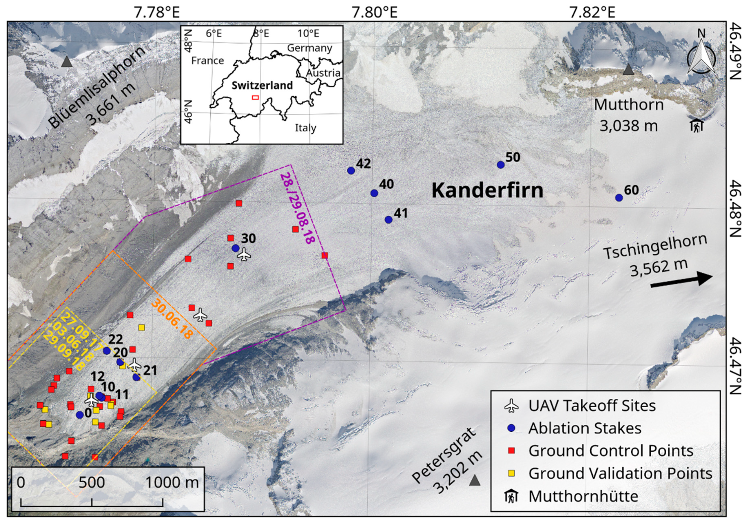
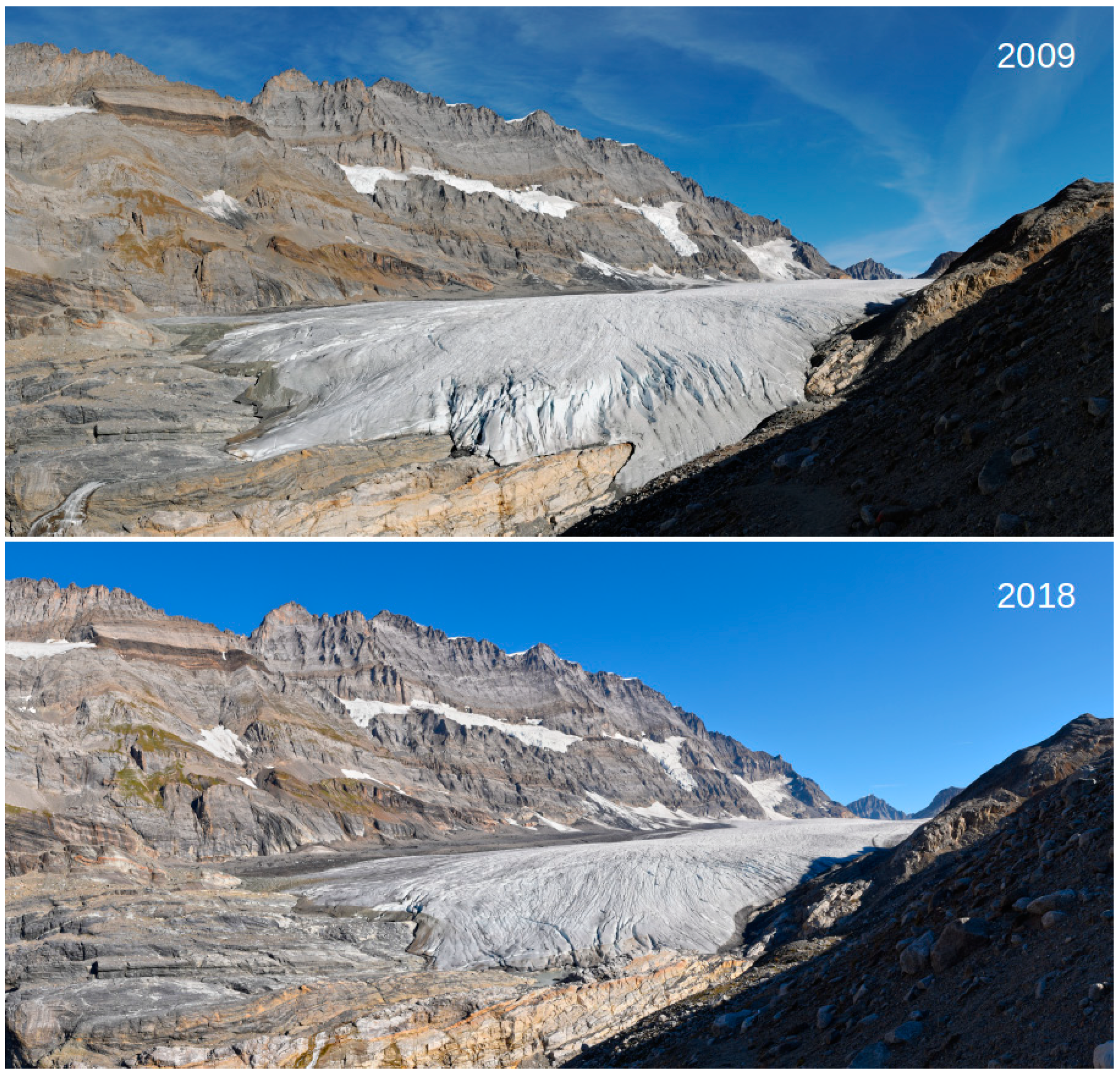
2. Study Site
3. Materials and Methods
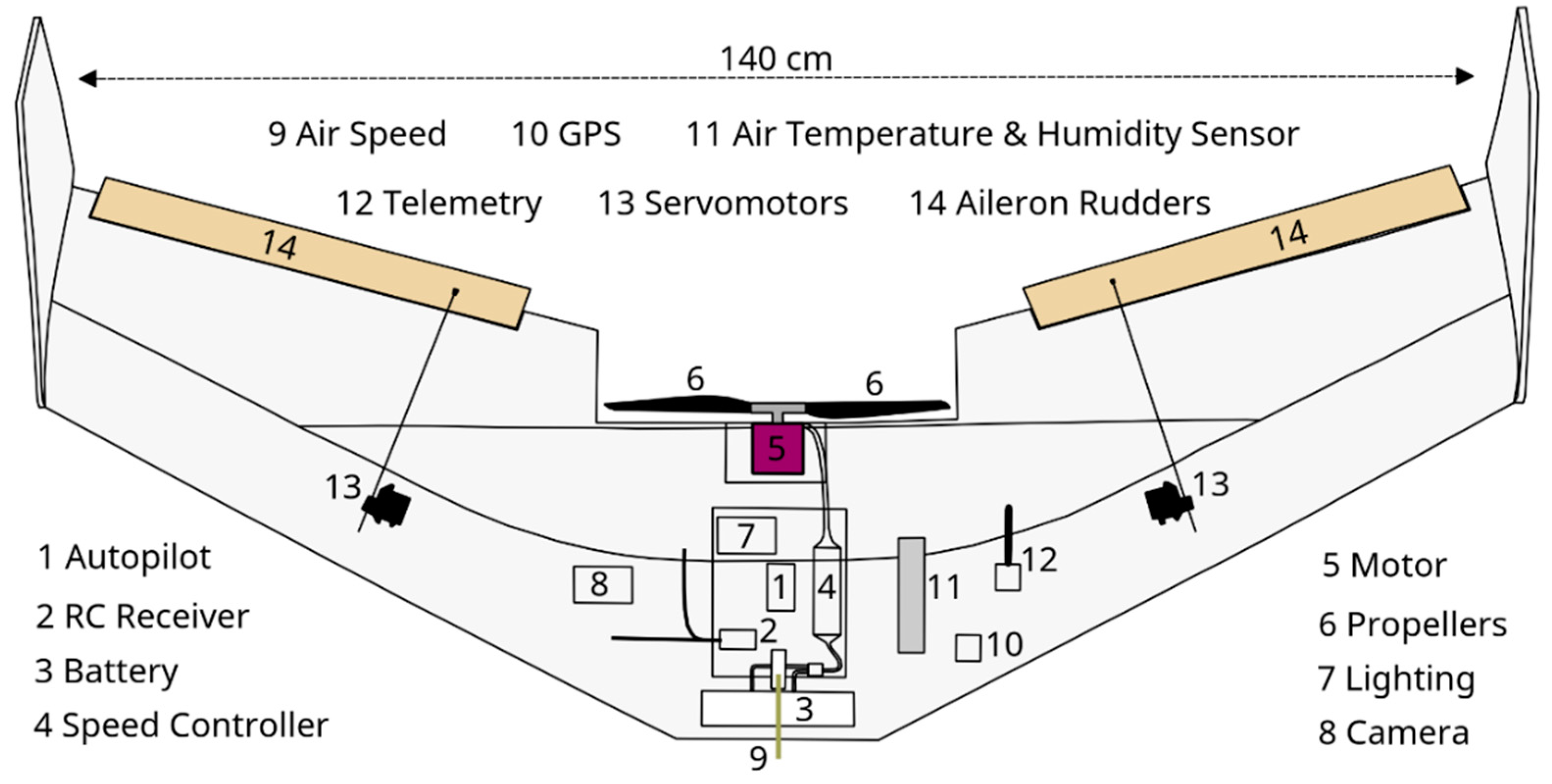
3.1. Unmanned Aircraft System
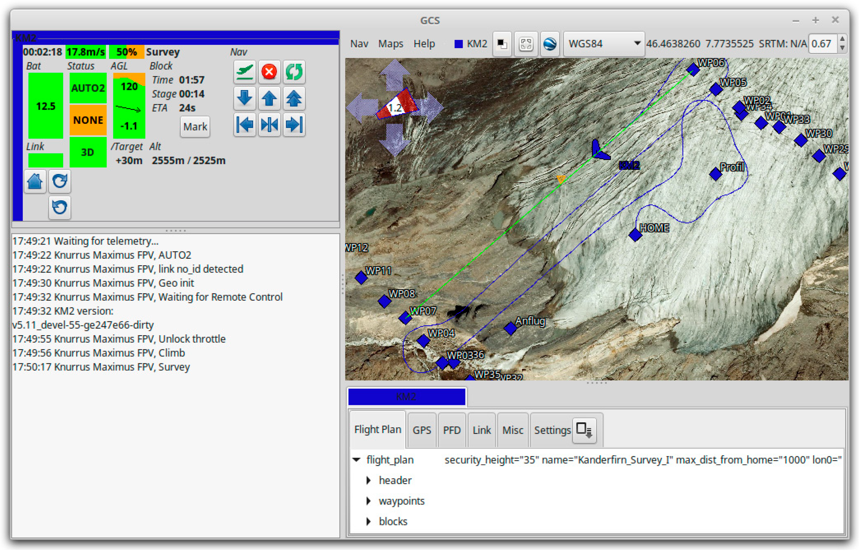
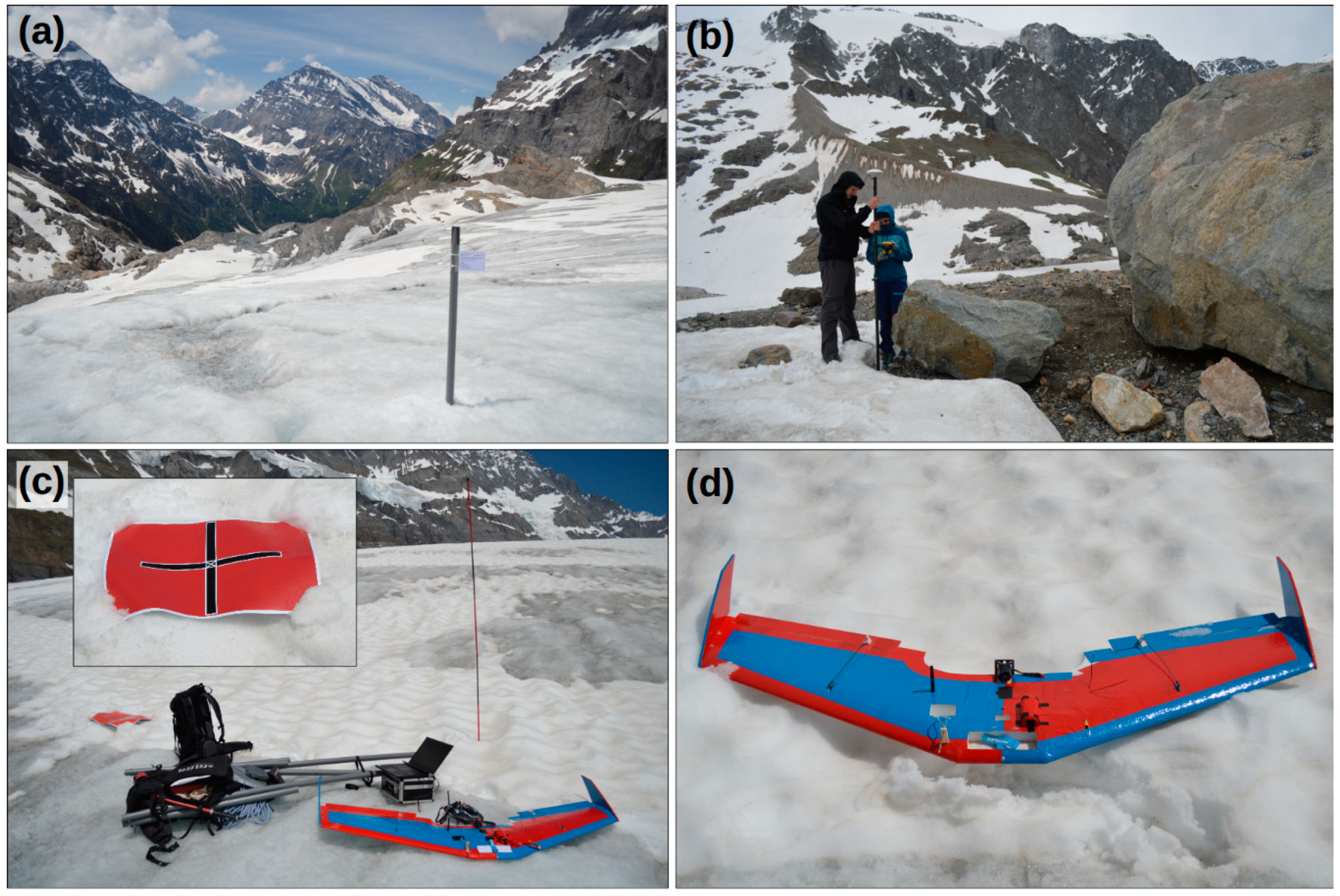
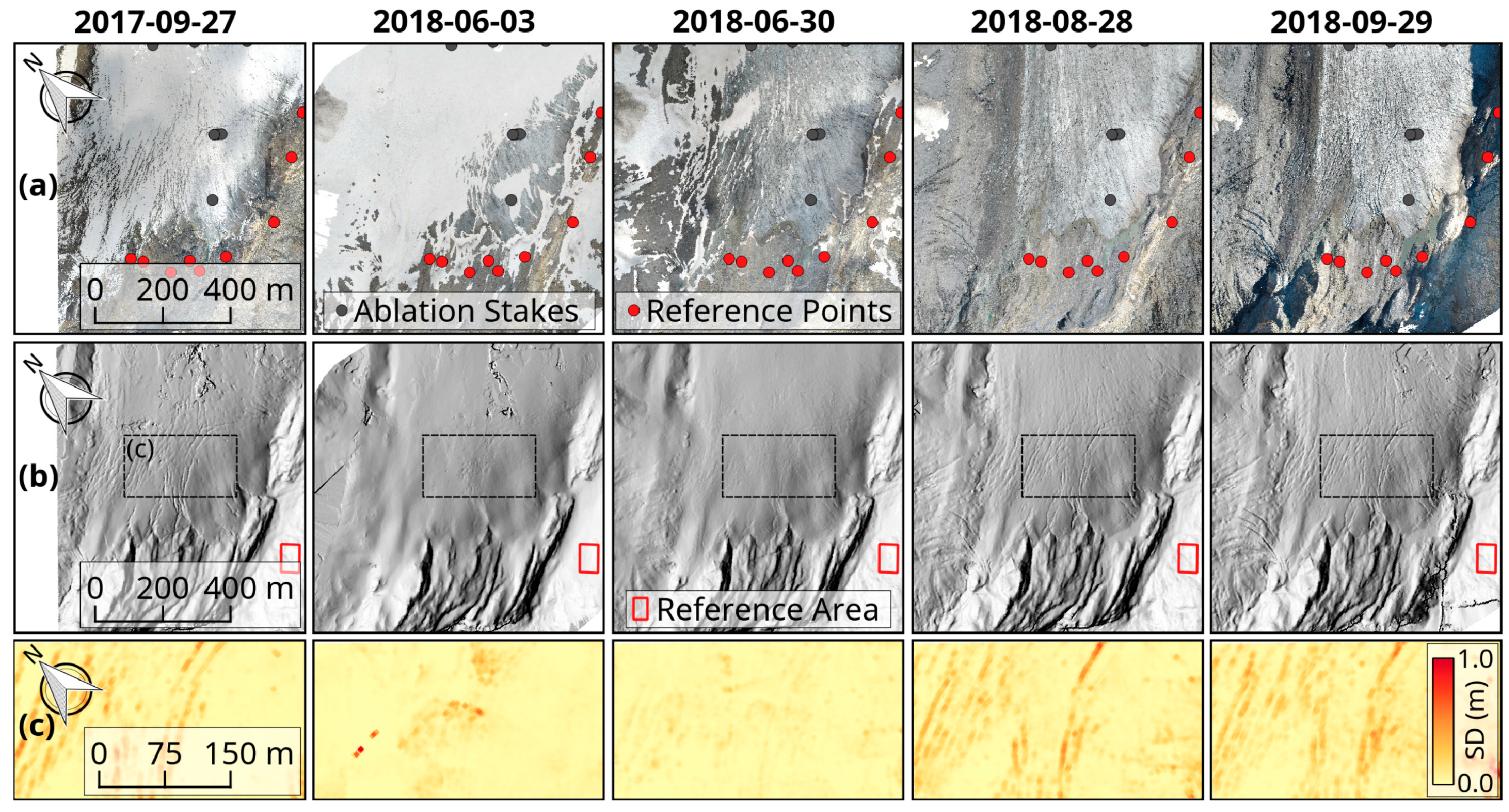
3.2. Aerial Surveys and In-Situ Measurements
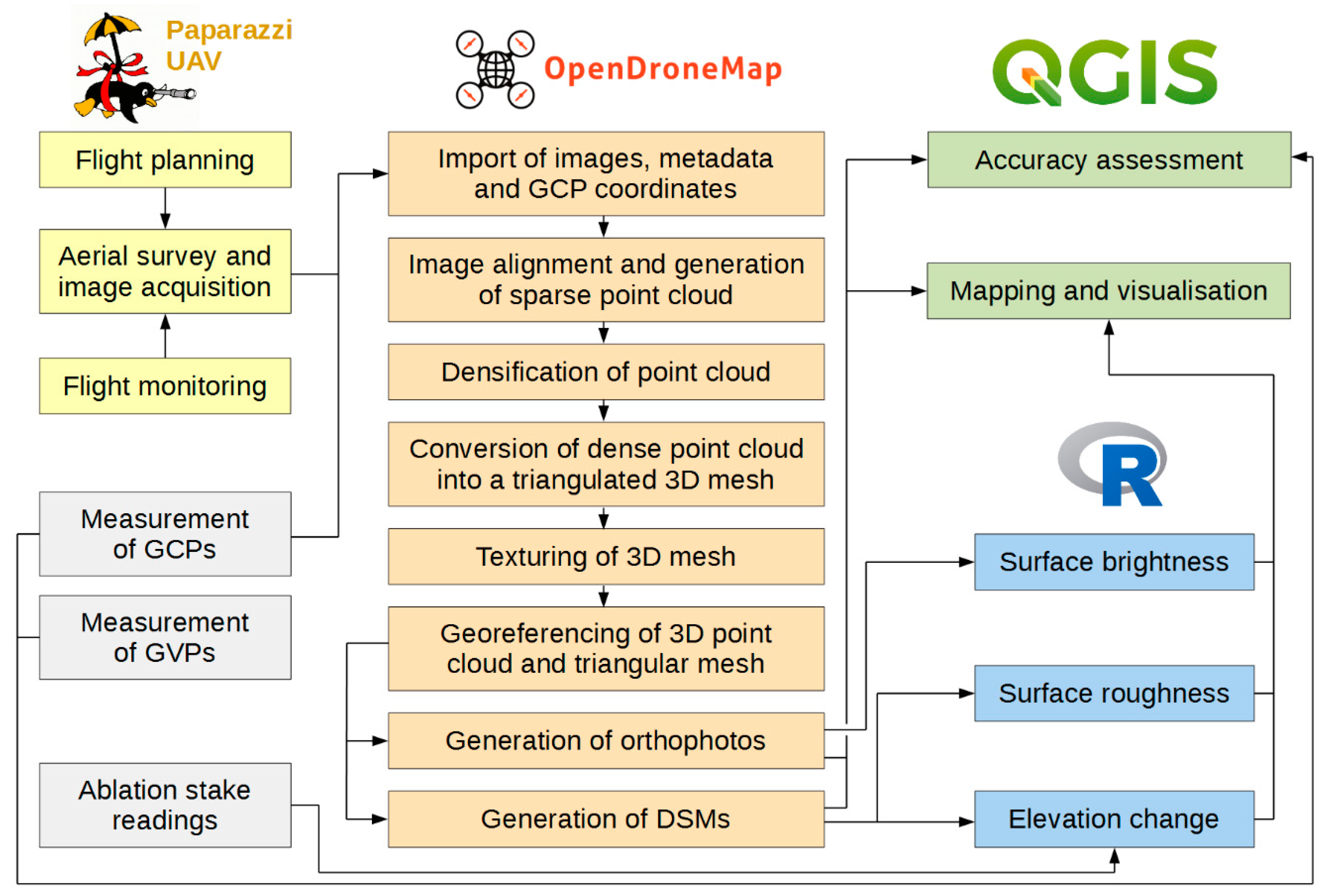
3.3. Generation of Orthophotos and DSMs
- Import of (geotagged) aerial images and extraction of image metadata (camera specifications and geographical information).
- Calculation of accurate camera positions/orientations and generation of a sparse three-dimensional (3D) point cloud using the structure from motion library OpenSfM that performs feature extraction and matching [43].
- Densification of sparse point cloud based on Multi-View Stereo 3D reconstructions [44].
- Conversion of dense point cloud into a triangular 3D mesh based on an implemented Poisson Surface Reconstruction [45].
- Texturing of 3D mesh using an algorithm for large-scale 3D reconstructions. As data input, the algorithm requires a triangulated 3D mesh and images that are registered against this model [46].
- Georeferencing of 3D point cloud and triangular mesh. An affine transformation with three GCPs is applied to align the 3D models. For the affine transformation, OpenDroneMap chooses a combination of three GCPs that yields the highest possible accuracy.
- Generation of a georeferenced DSM from the dense point cloud.
- Generation of a georeferenced orthophoto from the textured mesh.
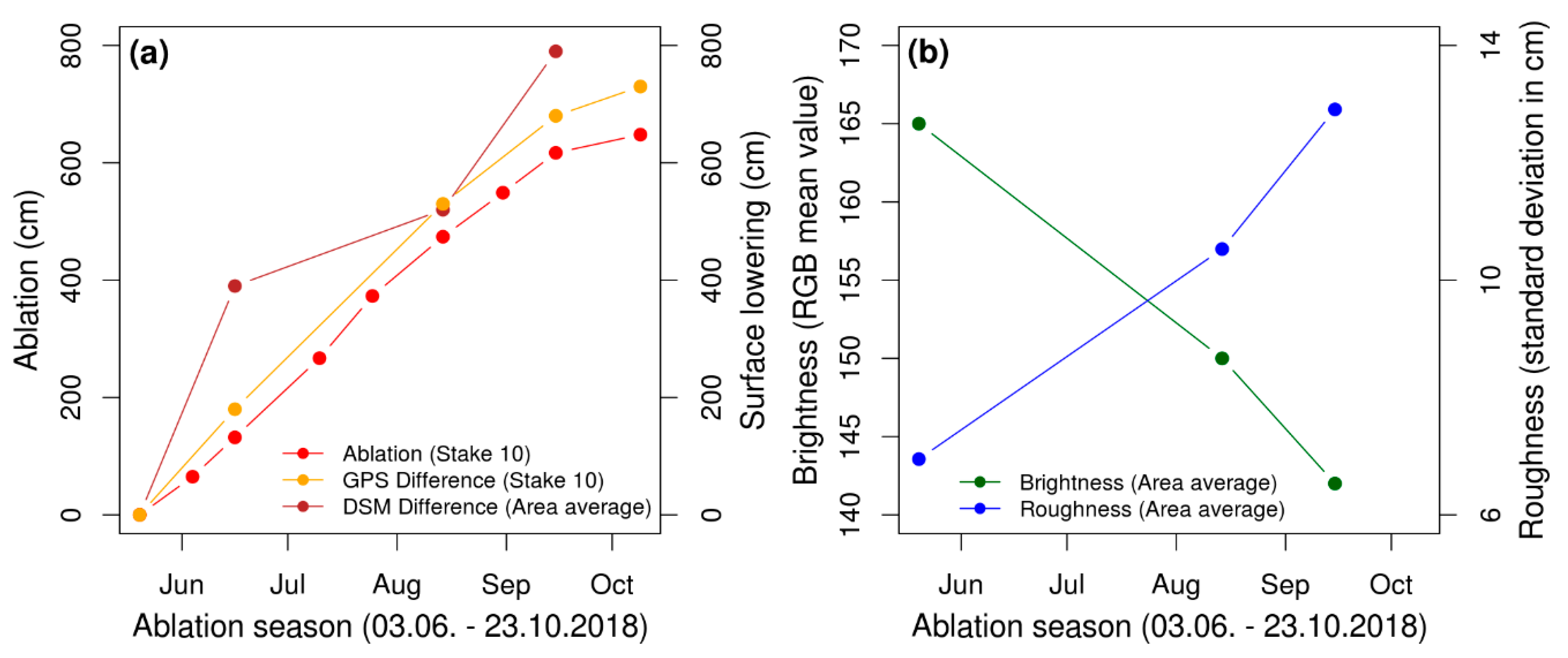
3.4. Calculation of Surface Brightness, Roughness and Elevation Changes
3.5. Quality Assessment
4. Results
4.1. Performance of UAV
4.2. Accuracy of Orthophotos and DSMs
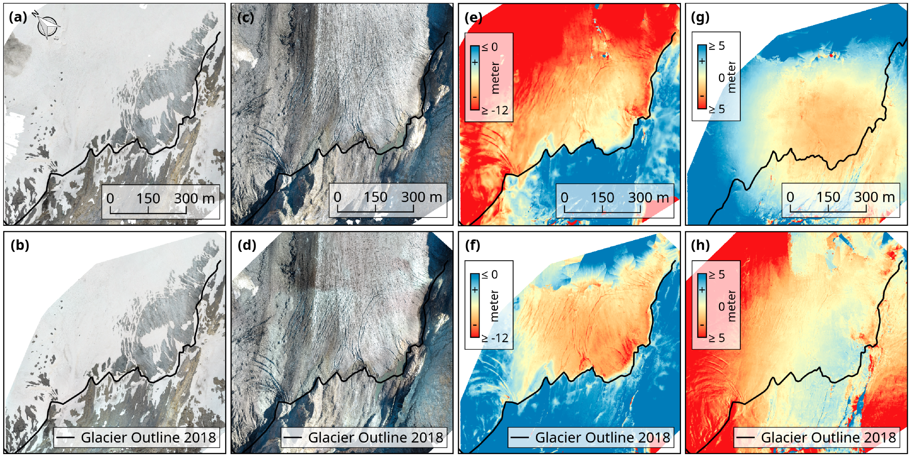
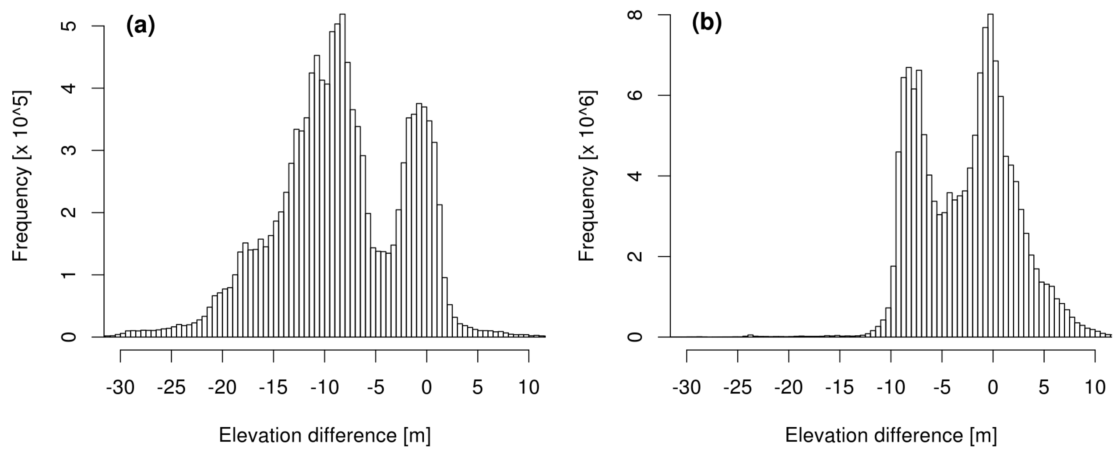
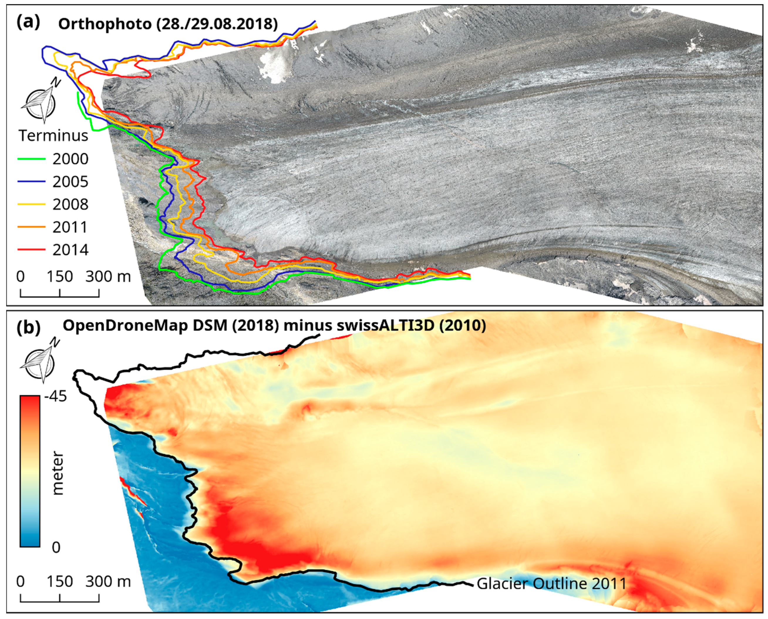
4.3. Glacier Surface Changes
5. Discussion
6. Conclusions
Data
Supplementary Materials
Author Contributions
Funding
Acknowledgments
Conflicts of Interest
Appendix A


| UAS Component | Manufacturer | Product | Cost (€) |
|---|---|---|---|
| Flying Wing | EPP-Versand | Knurrus Maximus FPV (140 cm) | 65 |
| Autopilot | Paparazzi UAV | Apogee v.1.0 | 150 |
| Remote Control | Graupner | HoTT mx-16, 2.4 GHz, incl. Receiver | 285 |
| Telemetry Modems | SparkFun | 2 x Xbee Pro S2B 2.4 Ghz, incl. Antenna | 130 |
| Motor | NTM Prop Drive | Series 35-42A 1250Kv 600W | 30 |
| Speed Controler | Turnigy | Plush 60A Speed Controller | 50 |
| Propellers | Aero-Naut | 2 x CAM-Carb. 12 × 6‘‘ Folding Propeller | 10 |
| Servo Motors | Multiplex | 2 x Hitec Digital Servos (HS-5245MG) | 70 |
| GPS | Navilock | GPS | 30 |
| Battery | SLS | XTRON 5000mAh 3S1P 11.1V 20C/40C | 50 |
| Camera | GoPro | Hero 5 Black | 430 |
| Date | Software | Version | XY RMSE (m) | Z RMSE (m) |
|---|---|---|---|---|
| 27 September 2017 | ODM | 0.4.1 | 2.5 | 2.0 |
| 3 June 2018 | ODM | 0.4.1 | 0.8 | 1.5 |
| 3 June 2018 | Pix4D | 4.3.31 | 0.9 | 1.8 |
| 30 June 2018 | ODM | 0.4.1 | 0.6 | 0.8 |
| 28/29 August 2018 | ODM | 0.4.1 | 1.2 | 3.4 |
| 29 September 2018 | ODM | 0.4.1 | 0.9 | 0.6 |
| 29 September 2018 | Pix4D | 4.3.31 | 0.7 | 3.3 |
References
- Kaser, G.; Cogley, J.G.; Dyurgerov, M.B.; Meier, M.F.; Ohmura, A. Mass Balance of Glaciers and Ice Caps: Consensus Estimates for 1961–2004. Geophys. Res. Lett. 2006, 33, 1–5. [Google Scholar] [CrossRef]
- Zemp, M.; Frey, H.; Gärtner-Roer, I.; Nussbaumer, S.U.; Hoelzle, M.; Paul, F.; Haeberli, W.; Denzinger, F.; Ahlstrøm, A.P.; Anderson, B.; et al. Historically Unprecedented Global Glacier Decline in the Early 21st Century. J. Glaciol. 2015, 61, 745–762. [Google Scholar] [CrossRef]
- Marzeion, B.; Jarosch, A.H.; Hofer, M. Past and Future Sea-Level Change from the Surface Mass Balance of Glaciers. Cryosphere 2012, 6, 1295–1322. [Google Scholar] [CrossRef]
- Gardner, A.S.; Moholdt, G.; Cogley, J.G.; Wouters, B.; Arendt, A.A.; Wahr, J.; Berthier, E.; Hock, R.; Pfeffer, W.T.; Kaser, G.; et al. A Reconciled Estimate of Glacier Contributions to Sea Level Rise: 2003 to 2009. Science 2013, 340, 852–857. [Google Scholar] [CrossRef] [PubMed]
- Gregory, J.M.; White, N.J.; Church, J.A.; Bierkens, M.F.P.; Box, J.E.; van den Broeke, M.R.; Cogley, J.G.; Fettweis, X.; Hanna, E.; Huybrechts, P.; et al. Twentieth-Century Global-Mean Sea Level Rise: Is the Whole Greater than the Sum of the Parts? J. Clim. 2013, 26, 4476–4499. [Google Scholar] [CrossRef]
- Immerzeel, W.W.; van Beek, L.P.H.; Bierkens, M.F.P. Climate Change Will Affect the Asian Water Towers. Science 2010, 328, 1382–1385. [Google Scholar] [CrossRef] [PubMed]
- Kaser, G.; Großhauser, M.; Marzeion, B. Contribution Potential of Glaciers to Water Availability in Different Climate Regimes. Proc. Natl. Acad. Sci. USA 2010, 107, 20223–20227. [Google Scholar] [CrossRef] [PubMed]
- Huss, M.; Hock, R. Global-Scale Hydrological Response to Future Glacier Mass Loss. Nat. Clim. Chang. 2018, 135–140. [Google Scholar] [CrossRef]
- Haeberli, W.; Cihlar, J.; Barry, R.G. Glacier Monitoring within the Global Climate Observing System. Ann. Glaciol. 2000, 31, 241–246. [Google Scholar] [CrossRef]
- Braithwaite, R.J. Glacier Mass Balance: The First 50 Years of International Monitoring. Prog. Phys. Geogr. 2002, 26, 76–95. [Google Scholar] [CrossRef]
- Kääb, A.; Huggel, C.; Fischer, L.; Guex, S.; Paul, F.; Roer, I.; Salzmann, N.; Schlaefli, S.; Schmutz, K.; Schneider, D.; et al. Remote Sensing of Glacier-and Permafrost-Related Hazards in High Mountains: An Overview. Nat. Hazards Earth Syst. Sci. 2005, 5, 527–554. [Google Scholar] [CrossRef]
- Fischer, M.; Huss, M.; Hoelzle, M. Surface Elevation and Mass Changes of All Swiss Glaciers 1980–2010. Cryosphere 2015, 9, 525–540. [Google Scholar] [CrossRef]
- Whitehead, K.; Hugenholtz, C. Remote Sensing of the Environment with Small Unmanned Aircraft Systems (UASs), Part 1: A Review of Progress and Challenges. NRC Res. Press 2014, 2, 69–86. [Google Scholar] [CrossRef]
- Bhardwaj, A.; Sam, L.; Akanksha; Martín-Torres, F.J.; Kumar, R. UAVs as Remote Sensing Platform in Glaciology: Present Applications and Future Prospects. Remote Sens. Environ. 2016, 175, 196–204. [Google Scholar] [CrossRef]
- Fugazza, D.; Senese, A.; Azzoni, R.S.; Smiraglia, C.; Cernuschi, M.; Severi, D.; Diolaiuti, G. High Resolution Mapping of Glacier Surface Features. The UAV Survey of the Forni Glacier (Stelvio National Park, Italy). Geogr. Fis. Dinam. Quat. 2015, 28, 25–33. [Google Scholar]
- Fugazza, D.; Scaioni, M.; Corti, M.; D’Agata, C.; Agata, C.; Azzoni, R.S.; Cernuschi, M.; Smiraglia, C.; Diolaiuti, G.A. Combination of UAV and Terrestrial Photogrammetry to Assess Rapid Glacier Evolution and Map Glacier Hazards. Nat. Hazards Earth Syst. Sci. 2018, 18, 1055–1071. [Google Scholar] [CrossRef]
- Rippin, D.M.; Pomfret, A.; King, N. High Resolution Mapping of Supra-Glacial Drainage Pathways Reveals Link between Micro-Channel Drainage Density, Surface Roughness and Surface Reflectance: UAVs, SfM and Supra-Glacial Drainage. Earth Surf. Processes Landf. 2015, 40, 1–12. [Google Scholar] [CrossRef]
- Rossini, M.; Di Mauro, B.; Garzonio, R.; Baccolo, G.; Cavallini, G.; Mattavelli, M.; De Amicis, M.; Colombo, R. Rapid Melting Dynamics of an Alpine Glacier with Repeated UAV Photogrammetry. Geomorphology 2018, 304, 159–172. [Google Scholar] [CrossRef]
- Immerzeel, W.W.; Kraaijenbrink, P.D.A.; Shea, J.M.; Shrestha, A.B.; Pellicciotti, F.; Bierkens, M.F.P.; de Jong, S.M. High-Resolution Monitoring of Himalayan Glacier Dynamics Using Unmanned Aerial Vehicles. Remote Sens. Environ. 2014, 150, 93–103. [Google Scholar] [CrossRef]
- Kraaijenbrink, P.D.A.; Shea, J.M.; Pellicciotti, F.; de Jong, S.M.; Immerzeel, W.W. Object-Based Analysis of Unmanned Aerial Vehicle Imagery to Map and Characterise Surface Features on a Debris-Covered Glacier. Remote Sens. Environ. 2016, 186, 581–595. [Google Scholar] [CrossRef]
- Kraaijenbrink, P.; Meijer, S.W.; Shea, J.M.; Pellicciotti, F.; De Jong, S.M.; Immerzeel, W.W. Seasonal Surface Velocities of a Himalayan Glacier Derived by Automated Correlation of Unmanned Aerial Vehicle Imagery. Ann. Glaciol. 2016, 57, 103–113. [Google Scholar] [CrossRef]
- Kraaijenbrink, P.D.A.; Shea, J.M.; Litt, M.; Steiner, J.F.; Treichler, D.; Koch, I.; Immerzeel, W.W. Mapping Surface Temperatures on a Debris-Covered Glacier with an Unmanned Aerial Vehicle. Front. Earth Sci. 2018, 6, 1–19. [Google Scholar] [CrossRef]
- Ryan, J.C.; Hubbard, A.L.; Box, J.E.; Todd, J.; Christoffersen, P.; Carr, J.R.; Holt, T.O.; Snooke, N. UAV Photogrammetry and Structure from Motion to Assess Calving Dynamics at Store Glacier, a Large Outlet Draining the Greenland Ice Sheet. Cryosphere 2015, 9, 1–11. [Google Scholar] [CrossRef]
- Jouvet, G.; Weidmann, Y.; Seguinot, J.; Funk, M.; Abe, T.; Sakakibara, D.; Seddik, H.; Sugiyama, S. Initiation of a Major Calving Event on the Bowdoin Glacier Captured by UAV Photogrammetry. Cryosphere 2017, 11, 911–921. [Google Scholar] [CrossRef]
- Mayer, S.; Sandvik, A.; Jonassen, M.O.; Reuder, J. Atmospheric Profiling with the UAS SUMO: A New Perspective for the Evaluation of Fine-Scale Atmospheric Models. Meteorol. Atmos. Phys. 2012, 116, 15–26. [Google Scholar] [CrossRef]
- Cassano, J.J. Observations of Atmospheric Boundary Layer Temperature Profiles with a Small Unmanned Aerial Vehicle. Antarct. Sci. 2014, 26, 205–213. [Google Scholar] [CrossRef]
- Hattenberger, G.; Bronz, M.; Gorraz, M. Using the Paparazzi UAV System for Scientific Research. In Proceedings of the IMAV 2014, International Micro Air Vehicle Conference and Competition, Delft, The Netherlands, 12–15 August 2014; pp. 247–252. [Google Scholar]
- GitHub—OpenDroneMap/ODM. Available online: https://github.com/OpenDroneMap/ODM/ (accessed on 15 May 2019).
- Pix4D, SA. Pix4Dmapper 4.1 User Manual; Pix4D: Lausanne, Switzerland, 2017. [Google Scholar]
- Maisch, M.; Wipf, A.; Denneler, B.; Battaglia, J.; Benz, C. Die Gletscher der Schweizer Alpen: Gletscherhochstand 1850, Aktuelle Vergletscherung, Gletscherschwund-Szenarien (Schlussbericht NFP 31), 2nd ed.; Vdf-Verlag: Zurich, Switzerland, 2000. [Google Scholar]
- Paul, F. The New Swiss Glacier Inventory 2000—Application of Remote Sensing and GIS. Ph.D. Thesis, Department of Geography, University of Zurich, Zurich, Switzerland, 2004. [Google Scholar]
- Müller, F.; Caflisch, T.; Müller, G. Firn und Eis der Schweizer Alpen (Gletscherinventar), Publ. Nr. 57/57a; ETH Zurich: Zurich, Switzerland, 1976. [Google Scholar]
- Fischer, M.; Huss, M.; Barboux, C.; Hoelzle, M. The New Swiss Glacier Inventory SGI2010: Relevance of Using High-Resolution Source Data in Areas Dominated by Very Small Glaciers. Arct. Antarc. Alp. Res. 2014, 46, 933–945. [Google Scholar] [CrossRef]
- GLAMOS. Swiss Glacier Length Change (Release 2018); Glacier Monitoring Switzerland: Zurich, Switzerland, 2018. [Google Scholar]
- Farinotti, D.; Huss, M.; Bauder, A.; Funk, M. An Estimate of the Glacier Ice Volume in the Swiss Alps. Glob. Planet. Chang. 2009, 68, 225–231. [Google Scholar] [CrossRef]
- Rutishauser, A.; Maurer, H.; Bauder, A. Helicopter-Borne Ground-Penetrating Radar Investigations on Temperate Alpine Glaciers: A Comparison of Different Systems and Their Abilities for Bedrock Mapping. Geophysics 2016, 81, 119–129. [Google Scholar] [CrossRef]
- Linsbauer, A.; Paul, F.; Haeberli, W. Modeling Glacier Thickness Distribution and Bed Topography over Entire Mountain Ranges with GlabTop: Application of a Fast and Robust Approach. J. Geophys. Res. F Earth Surf. 2012, 117, 1–17. [Google Scholar] [CrossRef]
- Huss, M.; Dhulst, L.; Bauder, A. New Long-Term Mass-Balance Series for the Swiss Alps. J. Glaciol. 2015, 61, 551–562. [Google Scholar] [CrossRef]
- Kaser, G.; Fountain, A.; Jansson, P. A Manual for Monitoring the Mass Balance of Mountain Glaciers with Particular Attention to Low Latitude Characteristics; A Contribution from the International Commission on Snow and Ice (ICSI) to the UNESCO HKH-Friend Programme, IHP-VI, Technical Documents in Hydrology, No. 59; UNSECO: Paris, France, 2003. [Google Scholar]
- GoPro. Hero Black 5 User Manual; GoPro: San Mateo, CA, USA, 2017. [Google Scholar]
- Trimble. Geo 7X Handheld User Guide; Trimble: Sunnyvale, CA, USA, 2013. [Google Scholar]
- GitHub—OpenDroneMap/WebODM. Available online: https://github.com/OpenDroneMap/WebODM (accessed on 15 May 2019).
- GitHub—OpenSfM. Available online: https://github.com/mapillary/OpenSfM (accessed on 15 May 2019).
- Shen, S. Accurate Multiple View 3D Reconstruction Using Patch-Based Stereo for Large-Scale Scenes. IEEE Trans. Image Process. 2013, 22, 1901–1914. [Google Scholar] [CrossRef]
- Bolitho, M.; Kazhdan, M.; Burns, R.; Hoppe, H. Parallel Poisson Surface Reconstruction. In Advances in Visual Computing, 5th International Symposium; Bebis, G., Boyle, R., Parvin, B., Koracin, D., Kuno, Y., Wang, J., Wang, J., Wang, J., Pajarola, R., Lindstrom, P., et al., Eds.; Springer: Berlin/Heidelberg, Germany, 2009; Volume 1, pp. 678–689. [Google Scholar]
- Waechter, M.; Moehrle, N.; Goesele, M. Let There Be Color! Large-Scale Texturing of 3D Reconstructions. In Computer Vision—ECCV 2014, 13th European Conference; Fleet, D., Pajdla, T., Schiele, B., Tuytelaars, T., Eds.; Springer: Berlin/Heidelberg, Germany, 2014; Volume 5, pp. 836–851. [Google Scholar]
- OpenDroneMap’s Documentation. Available online: https://docs.opendronemap.org/using.html#ground-control-points (accessed on 15 May 2019).
- Hock, R. Glacier Melt: A Review of Processes and Their Modelling. Prog. Phys. Geogr. 2005, 29, 362–391. [Google Scholar] [CrossRef]
- Ryan, J.C.; Hubbard, A.; Box, J.E.; Brough, S.; Cameron, K.; Cook, J.M.; Cooper, M.; Doyle, S.H.; Edwards, A.; Holt, T.; et al. Derivation of High Spatial Resolution Albedo from UAV Digital Imagery: Application over the Greenland Ice Sheet. Front. Earth Sci. 2017, 5, 1–13. [Google Scholar] [CrossRef]
- Corripio, J.G. Snow Surface Albedo Estimation Using Terrestrial Photography. Int. J. Remote Sens. 2004, 25, 5705–5729. [Google Scholar] [CrossRef]
- Smith, M.W.; Quincey, D.J.; Dixon, T.; Bingham, R.G.; Carrivick, J.L.; Irvine-Fynn, T.D.L.; Rippin, D.M. Aerodynamic Roughness of Glacial Ice Surfaces Derived from High-Resolution Topographic Data. J. Geophys. Res. F Earth Surf. 2016, 121, 748–766. [Google Scholar] [CrossRef]
- Miles, E.S.; Steiner, J.F.; Brun, F. Highly Variable Aerodynamic Roughness Length (Z0) for a Hummocky Debris-Covered Glacier. J. Geophys. Res. Atmos 2017, 122, 8447–8466. [Google Scholar] [CrossRef]
- Shepard, M.K.; Campbell, B.A.; Bulmer, M.H.; Farr, T.G.; Gaddis, L.R.; Plaut, J.J. The Roughness of Natural Terrain: A Planetary and Remote Sensing Perspective. J. Geophys. Res. 2001, 106, 32777–32795. [Google Scholar] [CrossRef]
- QGIS Documentation. Available online: https://www.qgis.org/en/docs/index.html (accessed on 15 May 2019).
- Swiss Federal Office of Topography. SWISSIMAGE—Das Digitale Farborthophotomosaik der Schweiz; SwissTopo Wabern: Knitz, Switzerland, 2010. [Google Scholar]
- Swiss Federal Office of Topography. SwissALTI3D—Das Hoch Aufgelöste Terrainmodell der Schweiz; SwissTopo Wabern: Knitz, Switzerland, 2018. [Google Scholar]
- Gindraux, S.; Boesch, R.; Farinotti, D. Accuracy Assessment of Digital Surface Models from Unmanned Aerial Vehicles’ Imagery on Glaciers. Remote Sens. 2017, 9, 186. [Google Scholar] [CrossRef]
- Paparazzi UAV Wiki. Available online: https://wiki.paparazziuav.org/wiki/Main_Page (accessed on 15 May 2019).
- James, M.R.; Robson, S. Mitigating systematic error in topographic models derived from UAV and ground based image networks. Earth Surf. Processes Landf. 2014, 39, 1413–1420. [Google Scholar] [CrossRef]
- Balletti, C.; Guerra, F.; Tsioukas, V.; Vernier, P. Calibration of Action Cameras for Photogrammetric Purposes. Sensors 2014, 14, 17471–17490. [Google Scholar] [CrossRef]
- GitHub Discussion on Geoferencing and Image Alignment in OpenDroneMap. Available online: https://github.com/OpenDroneMap/ODM/pull/947 (accessed on 15 May 2019).
- Bühler, Y.; Adams, M.S.; Bösch, R.; Stoffel, A. Mapping snow depths in alpine terrain with unmanned aerial systems (UASs): Potential and limitations. Cryosphere 2016, 10, 1075–1088. [Google Scholar] [CrossRef]
- Chudley, T.R.; Christoffersen, P.; Doyle, S.H.; Abellan, A.; Snooke, N. High-accuracy UAV photogrammetry of ice sheet dynamics with no ground control. Cryosphere 2019, 13, 955–968. [Google Scholar] [CrossRef]


| Date | Flight No. | Start Time (hh:mm) | Flight Time (hh:mm) | Flight Altitude (m a.g.l.) | Area (km²) | Images (selected) | Resolution (cm/pixel) |
|---|---|---|---|---|---|---|---|
| 27 September 2017 | 1 | 16:26 | 00:14 | 140 ± 10 | 0.7 | 1242 (314) | 7.2 ± 0.5 |
| 3 June 2018 | 1 | 14:37 | 00:16 | 140 ± 10 | 0.7 | 913 (347) | 7.2 ± 0.5 |
| 30 June 2018 | 1 | 15:03 | 00:16 | 120 ± 10 | 0.8 | 972 (249) | 6.2 ± 0.5 |
| 30 June 2018 | 2 | 18:02 | 00:16 | 135 ± 20 | 0.8 | 952 (228) | 6.9 ± 1.0 |
| 28 August 2018 | 1 | 13:27 | 00:15 | 120 ± 10 | 0.8 | 883 (210) | 6.2 ± 0.5 |
| 28 August 2018 | 2 | 15:24 | 00:16 | 135 ± 20 | 0.8 | 935 (210) | 6.9 ± 1.0 |
| 28 August 2018 | 3 | 17:14 | 00:17 | 135 ± 20 | 0.8 | 992 (217) | 6.9 ± 1.0 |
| 29 August 2018 | 1 | 12:20 | 00:17 | 135 ± 20 | 0.8 | 1036 (213) | 6.9 ± 1.0 |
| 29 September 2018 | 1 | 10:51 | 00:11 | 120 ± 10 | 0.8 | 668 (215) | 6.2 ± 0.5 |
| 29 September 2018 | 2 | 16:15 | 00:01 | 120 ± 10 | <0.1 | 70 (0) | 6.2 ± 0.5 |
| Stake | Lat (°N) | Lon (°E) | Elevation (m) | Start Date | End Date | Period (d) | Ablation (cm) | Ablation (cm d−1) |
|---|---|---|---|---|---|---|---|---|
| 00 | 46.4663 | 7.7735 | 2363 | 30 June 2018 13:00 | 23 October 2018 11:40 | 114.9 | 549 | 4.8 |
| 10 | 46.4675 | 7.7754 | 2414 | 3 June 2018 15:00 | 23 October 2018 11:30 | 141.9 | 648 | 4.6 |
| 11 | 46.4674 | 7.7755 | 2413 | 3 June 2018 15:00 | 23 October 2018 11:25 | 141.9 | 610 | 4.3 |
| 12 | 46.4675 | 7.7752 | 2413 | 30 June 2018 11:50 | 23 October 2018 11:35 | 115.0 | 521 | 4.5 |
| 20 | 46.4697 | 7.7771 | 2444 | 30 June 2018 16:50 | 23 October 2018 11:00 | 114.8 | 443 | 3.9 |
| 21 | 46.4688 | 7.7786 | 2437 | 30 June 2018 16:15 | 23 October 2018 11:15 | 114.8 | 489 | 4.3 |
| 22 | 46.4704 | 7.7759 | 2446 | 30 June 2018 17:10 | 23 October 2018 11:05 | 114.7 | 509 | 4.4 |
| 30 | 46.4770 | 7.7875 | 2544 | 24 July 2018 14:15 | 23 October 2018 10:20 | 90.8 | 347 | 3.8 |
| 40 | 46.4807 | 7.8002 | 2633 | 8 August 2018 15:15 | 23 October 2018 09:50 | 75.8 | 204 | 2.7 |
| 41 | 46.4790 | 7.8016 | 2632 | 24 July 2018 15:30 | 23 October 2018 00:00 | 90.4 | 335 | 3.7 |
| 42 | 46.4821 | 7.7980 | 2641 | 8 August 2018 15:45 | 23 October 2018 09:45 | 75.8 | 284 | 3.7 |
| 50 | 46.4826 | 7.8118 | 2735 | 8 August 2018 16:30 | 23 October 2018 09:30 | 75.7 | 186 | 2.5 |
| 60 | 46.4806 | 7.8227 | 2843 | 9 August 2018 09:30 | 23 October 2018 09:00 | 75.0 | 136 | 1.8 |
| Date | Software | Version | GCPs | GVPs | XY RMSE (m) | Z RMSE (m) | ||||
|---|---|---|---|---|---|---|---|---|---|---|
| GCP | GVP | Total | GCP | GVP | Total | |||||
| 27 September 2017 | ODM | 0.4.1 | 5 | 4 | 1.3 | 1.1 | 1.2 | 1.0 | 0.6 | 0.9 |
| 3 June 2018 | ODM | 0.4.1 | 5 | 3 | 0.6 | 0.7 | 0.7 | 0.7 | 0.8 | 0.7 |
| 3 June 2018 | Pix4D | 4.3.31 | 5 | 3 | 0.3 | 0.7 | 0.5 | 0.3 | 0.3 | 0.4 |
| 30 June 2018 | ODM | 0.4.1 | 9 | 3 | 1.5 | 0.4 | 1.2 | 2.3 | 1.2 | 2.1 |
| 28./29 August 2018 | ODM | 0.4.1 | 22 | 5 | 1.3 | 0.9 | 1.2 | 2.1 | 0.9 | 1.9 |
| 29 September 2018 | ODM | 0.4.1 | 6 | 4 | 0.6 | 0.7 | 0.7 | 0.9 | 0.9 | 0.9 |
| 29 September 2018 | Pix4D | 4.3.31 | 6 | 4 | 0.2 | 0.4 | 0.3 | 0.2 | 0.7 | 0.5 |
© 2019 by the authors. Licensee MDPI, Basel, Switzerland. This article is an open access article distributed under the terms and conditions of the Creative Commons Attribution (CC BY) license (http://creativecommons.org/licenses/by/4.0/).
Share and Cite
Groos, A.R.; Bertschinger, T.J.; Kummer, C.M.; Erlwein, S.; Munz, L.; Philipp, A. The Potential of Low-Cost UAVs and Open-Source Photogrammetry Software for High-Resolution Monitoring of Alpine Glaciers: A Case Study from the Kanderfirn (Swiss Alps). Geosciences 2019, 9, 356. https://doi.org/10.3390/geosciences9080356
Groos AR, Bertschinger TJ, Kummer CM, Erlwein S, Munz L, Philipp A. The Potential of Low-Cost UAVs and Open-Source Photogrammetry Software for High-Resolution Monitoring of Alpine Glaciers: A Case Study from the Kanderfirn (Swiss Alps). Geosciences. 2019; 9(8):356. https://doi.org/10.3390/geosciences9080356
Chicago/Turabian StyleGroos, Alexander R., Thalia J. Bertschinger, Céline M. Kummer, Sabrina Erlwein, Lukas Munz, and Andreas Philipp. 2019. "The Potential of Low-Cost UAVs and Open-Source Photogrammetry Software for High-Resolution Monitoring of Alpine Glaciers: A Case Study from the Kanderfirn (Swiss Alps)" Geosciences 9, no. 8: 356. https://doi.org/10.3390/geosciences9080356
APA StyleGroos, A. R., Bertschinger, T. J., Kummer, C. M., Erlwein, S., Munz, L., & Philipp, A. (2019). The Potential of Low-Cost UAVs and Open-Source Photogrammetry Software for High-Resolution Monitoring of Alpine Glaciers: A Case Study from the Kanderfirn (Swiss Alps). Geosciences, 9(8), 356. https://doi.org/10.3390/geosciences9080356