Article

Methods to Invert Temperature Data and Heat Flow Data for Thermal Conductivity in Steady-State Conductive Regimes

by
Wallace Anderson McAliley
* and
Yaoguo Li
Center for Gravity, Electrical, and Magnetic Studies, Department of Geophysics, Colorado School of Mines, Golden, CO 80401, USA
*
Author to whom correspondence should be addressed.
Geosciences 2019, 9(7), 293; https://doi.org/10.3390/geosciences9070293
Submission received: 1 June 2019 / Revised: 27 June 2019 / Accepted: 28 June 2019 / Published: 3 July 2019
(This article belongs to the Special Issue Subsurface Thermography and the Use of Temperature in Geosciences)

Abstract

:
Temperature and heat flow data carry specific information about the distribution of thermal conductivity variations which is not available in other geophysical data sets. Thus, thermal data constitute important complementary data sets in the multiphysics-based imaging and characterization of earth’s subsurface. The quantitative interpretations that accompany this effort can be carried out by determining thermal conductivities from temperature or heat flow data. Towards this goal, we develop inversion methods based on Tikhonov regularization and numerical solution of the differential equations governing the steady-state heat equation. Numerical simulations using these methods yield insights into the information content in thermal data and indicate it is similar to that in potential-field data. We apply the temperature inversion method to borehole temperature data from the Cooper Basin in Australia, a well-studied geothermal prospect. The methods and insights presented in this study pave the way for imaging the subsurface through recovered thermal conductivities and for joint quantitative interpretations of thermal data with other common geophysical data sets in various geoscientific applications.

1. Introduction

Geoscientists use thermal data to solve problems in a variety of contexts, including petroleum basin temperature modeling, crustal-scale geoscience, geothermal energy and detecting groundwater flow [1,2,3,4]. Inversion provides a quantitative tool to aid data interpretation. While the research community often inverts thermal data using parametric approaches for interpretation, generalized inversion has not yet been applied to thermal data. Unlike parametric inversions, a generalized inversion seeks to recover an approximation to a function. Generalized inversion has successfully allowed geoscientists to effectively interpret geologic structure from gravity, magnetic, electrical and electromagnetic data. We present deterministic generalized inverse methods for thermal data, which allow for the recovery of general physical property distributions.
There are several ways to parameterize physical properties that have been used to invert thermal data for thermal conductivity. One technique is to predefine structural boundaries between lithologic units prior to inversion, assume that properties are constant within each lithologic unit and invert for the property values within each unit. The assumption of homogeneous properties within each unit reduces the number of parameters to be resolved, allowing the statistics of each parameter to be estimated via stochastic or Bayesian inversion. This approach is popular, as it easily allows different properties such as heat production rates, basal heat flow rates or hydraulic permeabilities to be simultaneously recovered alongside thermal conductivity [5,6,7,8]. Another approach is to assume a fixed property value for each predefined lithologic unit and invert for structural boundaries. While not as common, this approach has also been used to invert thermal data [9,10]. An approach that has been widely used to invert many different kinds of geophysical data is generalized deterministic inversion. In such an inversion, an earth model is finely discretized and physical property values are determined for each discrete model cell, usually by solving a regularized least-squares minimization problem. The methodological framework for applying generalize inversion to thermal data is well understood [11] and has been applied to resolve a small number of model parameters [12,13]. However, to our knowledge, no study has implemented generalized inversion to resolve a large number of thermal conductivity parameters, nor addressed the specifics of implementing such an inversion.
Here we present methods to invert temperature data and heat flow data for thermal conductivity by generalized deterministic inversion. First, we describe the finite volume method used to compute temperatures and heat flows in a steady-state conductive regime from a known thermal conductivity model, boundary conditions and heat sources. Next, we develop methods to invert temperature data and heat flow data for thermal conductivity in an efficient manner which allows a general thermal conductivity distribution to be recovered. We implement these methods in MATLAB and we apply them to invert borehole temperature data from the Cooper Basin, recovering both a thermal conductivity model and an estimate of subsurface temperatures in the region. We discuss the non-uniqueness inherent in these inverse problems and show synthetic examples of inversion results. We also discuss the challenges of thermal modeling and the assumptions required to implement this method.

2. Thermal Data Background

We examine the inversion of two kinds of thermal data: borehole temperature and surface heat flow. Borehole temperatures are usually measurements of the temperature of the bore fluid. They may be collected as part of a precision temperature log or as bottom-hole temperature measurements, which are measurements of the maximum temperature in a well taken during geophysical logging. Borehole temperature can be measured by a thermometer, a thermistor or by distributed temperature sensing technology which measures temperatures along the length of a fiber optic cable. This technology allows large amounts of temperature data to be collected relatively inexpensively [1].
The accuracy of borehole temperature measurements depends largely on whether the bore fluid is in thermal equilibrium. Borehole temperatures are strongly disturbed by drilling operations, especially mud circulation. Bottom-hole temperature measurements are usually collected soon after drilling, so those measurements are usually lower than the undisturbed temperature. Several methods have been developed to recover undisturbed formation temperatures from bottom-hole temperatures. See References [14,15,16,17] for comparisons of common correction techniques. In this work, we ignore the effects of drilling operations on temperature measurements and assume that the requisite data processing has been applied.
Heat flow measurements are made for the purposes of estimating the earth’s total heat budget, characterizing large-scale fluid movement, understanding or better characterizing seafloor spreading or resource exploration. Heat flow is not measured directly. Rather, the thermal gradient and the thermal conductivity are both measured and then heat flow can be determined from the two measurements. While heat flow can be measured both near the surface of the earth and deep in boreholes, we examine only heat flow data from the top few meters of the earth, referred to as surface heat flow. Surface heat flow is usually measured at sea. In deep ocean settings, the ocean bottom temperature is relatively constant because seawater is densest at 3.4 °C. Thus, steady-state assumptions are more justifiable at the seafloor than on land. Both the increased likelihood of a steady-state regime and the ease with which probes can penetrate the ocean bottom allow heat flow to be determined relatively quickly at the ocean floor. However, water movement can strongly influence the subsurface thermal field there. Heat flow can be measured at the land surface as well, although such measurements are susceptible to the effects of ground surface temperature fluctuations. They are usually taken over several days or weeks to account for temporal changes [1].
Temperatures and heat flow rates in the subsurface depend on conductive and convective heat transport, heat sources within the earth and past changes in the temperature field. Additionally, the temperature and topography of the surface of the earth and the rate of heat flow into the base of the lithosphere affect the temperature of the crust. These dependencies can be seen in the diffusive-advective heat transport equation,
ρ c p u t + · q a + q c = f ,
which governs how the temperature u depends upon the density ρ , specific heat c p , the time derivative of temperature u t , advective heat flow q a , conductive heat flow q c and the rate of heat production f. Here, advective heat flow refers to the rate of heat transport via movement of mass, including rock and fluid movement. Conductive heat flow, by contrast, is the rate of heat transport within materials that arises due to exchanges of kinetic energy among molecules. It flows in the direction of the temperature gradient, from hot to cold.
In this work we assume that the area is in thermal steady-state and that all heat flow is conductive. For these assumptions to be valid, several conditions must be met. Care must be taken to ensure that the thermal regime under study sufficiently meets these criteria.
Temperatures are not in steady-state in all regions of the subsurface. On land, fluctuations in ground surface temperature keep the shallow temperature field from reaching steady-state. Yearly temperature cycles affect the top few tens of meters [18]. Below that, annual temperature fluctuations do not affect the temperature significantly, although longer period temperature changes can affect deeper temperatures. Major paleoclimatic changes can cause thermal perturbations that extend kilometers into the subsurface. Therefore, the surface temperature history must be relatively constant and borehole temperatures should be measured at least 30 m below the surface. Furthermore, the region must be tectonically stable, as major fault movement can both generate heat through friction and transport it. Magma intrusions disturb the thermal steady-state as well. It may take thousands of years for steady-state to be recovered, depending on the intrusion size.
Beyond heat conduction, fluid movement in the subsurface is another important mechanism of heat transport that cannot always be neglected. The relative importance of advective heat flow over conductive heat flow can be quantified by the Peclet number,
P e = v L / κ ,
where v is the velocity of the fluid, L is the characteristic length of the advection process and κ is the thermal diffusivity of the rock-fluid complex. If P e < < 1 , then the effect of fluid advection can be safely ignored.
For the purposes of this study, we assume a steady-state, conductive regime in which the surface temperature, heat flow at depth and heat production sources are known or can be estimated. By applying these assumptions, Equation (1) is reduced to the steady-state heat equation, which we use to form the forward modeling operator.

3. Forward Modeling

The forward modeling operation solves for thermal data (either temperature or heat flow), given a thermal conductivity model, boundary conditions and heat sources, under the assumptions of purely conductive, steady-state heat transport and isotropic thermal conductivity.

3.1. Governing Equations

The steady-state heat equation,
· σ u = f ,
describes the behavior of the temperature field due to conductive heat transport alone under thermal equilibrium. Here, σ is thermal conductivity, u is temperature and f is the heat production rate per unit volume. Equation (3) can be constructed from two fundamental equations: the law of heat conduction,
q = σ u ,
where q is conductive heat flow (also known as heat flux density) and the law of conservation of energy,
· q = f .

3.2. Finite Volume Method

We solve Equation (3) by the finite volume method [19]. To derive the method, we integrate Equation (3) over a control volume V and apply the divergence theorem, yielding
S σ u · n ^ d s = V f d v ,
where S is the surface enclosing volume V and n ^ is a unit vector orthogonal to S, pointing outward. To implement the finite volume method, we discretize this equation.

3.3. Discretization

We discretize the model domain into rectilinear control volumes, known as cells. When discretized, the surface integral in Equation (6) becomes a summation over all the faces of the cell,
s σ s u · n ^ s a s = f V ,
where the index s corresponds to one of the faces, a s is the area of that face, u · n ^ s denotes the gradient of the temperature field in the direction of the outward normal vector at that face and V is the volume of the cell. We approximate the thermal conductivity within each cell by a single average value, located at the center of each cell. Temperatures and heat sources are also placed at cell centers. Heat flow values, being vector quantities, are located at cell faces since faces have inherent directionality.
For a rectilinear mesh, the gradient of the temperature at a cell face s in the direction normal to the face can be approximated by a finite difference between temperatures at cell centers on either side of the face, divided by the distance between cell centers:
u · n ^ s = u 2 u 1 ( Δ x 1 + Δ x 2 ) / 2 ,
where u 1 and u 2 are temperatures at the two cell centers and Δ x 1 and Δ x 2 are the widths of each cell in the direction normal to the face.
The thermal conductivity at a cell face must be interpolated from conductivities in each of the cells bordering the face. We use harmonic interpolation because it ensures heat flow continuity and thus conservation of energy [20]. So, if σ 1 and σ 2 are the thermal conductivities of the two cells that share face s, the conductivity at the cell face is estimated as
σ s = σ 1 σ 2 Δ x 1 + Δ x 2 σ 1 Δ x 2 + σ 2 Δ x 1 .
So, the term of the summation in Equation (7) corresponding to the face separating cells 1 and 2 is
2 σ 1 σ 2 a s σ 1 Δ x 2 + σ 2 Δ x 1 ( u 2 u 1 ) .
For a three-dimensional rectilinear mesh, there are six such terms in the equation corresponding to each control volume. Taken together, these equations form a linear system of equations. Ignoring boundary conditions, that system can be expressed in matrix-vector form as
G l T A s diag A v V σ 1 1 A s G l u = Vf ,
or, more simply,
G T MGu = Vf ,
where G is a discrete gradient operator matrix, M is a diagonal matrix that contains harmonically interpolated thermal conductivities, V is a diagonal matrix that contains the volume of each cell, u is a vector of temperatures at each cell center and f is a vector of heat source terms for each cell. See Appendix A for detailed definitions of these matrices and vectors.

3.4. Interpolating Fields

Once the temperature or heat flow fields have been computed, they must be interpolated to data locations. Many interpolation schemes may be used. For simplicity, we use trilinear interpolation. This interpolation method can be expressed as the product of an interpolation matrix Q and the vector of modeled field values s (be they temperatures or heat flow values), as
Qs = d ,
where d is a vector of field values interpolated to data locations.

3.5. Boundary Conditions

Boundary conditions are required to solve this boundary value problem. The thermal state of the earth can be modeled using different combinations of boundary conditions. For most geologic scenarios, the following boundary conditions are appropriate:
  • Known temperatures (Dirichlet boundary condition) are enforced at the top of the model.
  • The heat flow through the sides of the model is assumed to be zero (zero Neumann boundary condition).
  • At the base of the model, either the temperature (Dirichlet) or the vertical heat flow rate (Neumann) can be specified, depending on the situation being modeled. For example, the heat flow rate may be measured at the surface. If it is reasonable to assume that the horizontal variation of heat flow is negligible at depth, then a constant Neumann boundary condition is appropriate to use at the base of the model. The heat flow at the bottom of the model may be set to the average heat flow at the surface, subtracting the contributions of any known heat sources or sinks within the region of interest. Alternatively, a Dirichlet boundary condition may be desirable if there is information about temperatures at depth from other geophysical methods. This modeling approach can accommodate either type of boundary condition at any surface. For the examples in this study, we use a constant Neumann boundary condition at the base of the model.

3.5.1. Dirichlet Boundary Conditions

To impose a Dirichlet boundary condition at an exterior face, the values of σ s and u · n ^ s must be computed differently compared to Equations (8) and (9). For σ s , there is only one thermal conductivity since there is no neighboring cell, so no interpolation is necessary. The expression u · n ^ s is in this case a finite difference between the temperature at the center of the cell and the known temperature at the face, divided by the distance from cell center to the face,
u · n ^ s = u c e l l u B C Δ x c e l l / 2 .
In the linear system shown in Equation (12), these boundary conditions can be implemented at faces with Dirichlet boundary conditions as
G T M G u + G BC u BC = Vf ,
where u BC is a vector of Dirichlet boundary conditions and G BC is a gradient operator like G , matching the boundary temperatures to the correct face and direction with respect to the control volume.

3.5.2. Neumann Boundary Conditions

Neumann boundary conditions specify the normal derivative of the unknown quantity at the boundary. In geologic settings, however, we are more likely to have an estimate of the heat flow at a boundary than the temperature gradient. In this case that quantity is σ s u · n ^ s . Zero heat flow boundary conditions can be imposed at a face by setting the entry on the diagonal of B corresponding to the face to zero (see Appendix A). In addition, known heat flow values can be imposed at surfaces by constructing a vector q BC of known heat flow values and modifying Equation (15) to include it, as
G T M G u + G BC u BC q BC = Vf .

3.6. Solving for Temperature and Heat Flow

To solve Equation (16), we first move all known quantities to the right side to obtain
G T MGu = Vf G T M G BC u BC q BC .
This equation is now of the form of the linear system of equations
Au = b ,
where
A = G T M G b = V f G T M G BC u BC q BC
Note that all matrices in Equation (19) are sparse, and A is symmetric positive definite. Any number of linear solvers may be used to solve this system. Since it will be solved several times during the course of inversion, it is desirable to generate and save a preconditioner matrix P such that P 1 is an approximation to A 1 . The equation to solve becomes
P 1 Au = P 1 b
Since P 1 A has a smaller condition number than A , this system of equations is more conducive to numerical solvers. We employ incomplete Cholesky factorization to form a preconditioner and solve the system using the preconditioned conjugate gradient method [21].
Heat flow relates to temperature and conductivity through Equation (4), which can be expressed in a discrete form at the cell face separating cells 1 and 2 as
q s = σ s u · n ^ s , q s = 2 σ 1 σ 2 u 2 u 1 σ 1 Δ x 2 + σ 2 Δ x 1 .
Heat flow can be computed via
q = M G u + G BC u BC ,
where q is a vector of unknown heat flow values at centers of cell faces. Thus, once Equation (17) has been solved for u , Equation (22) can be solved for q .

3.7. Accuracy and Convergence
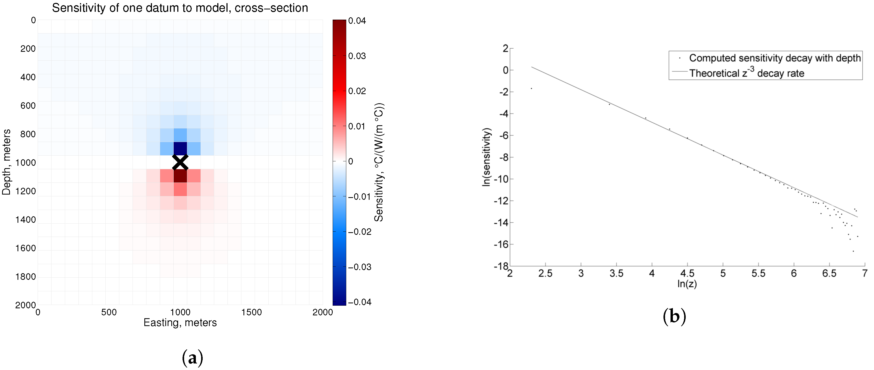
After implementing the finite volume algorithm in MATLAB, we constructed an analytic solution to verify the rate of convergence of the algorithm with increasingly fine mesh discretization. To produce the zero Neumann boundary conditions of the forward problem, we chose a spatially varying temperature field u over the domain of the unit cube, Ω = x , y , z : 0 x , y , z 1 , such that u x = 0 on x 0 , 1 and u y = 0 on y 0 , 1 :
u = 1 54 8 x 3 12 x 2 + 27 cos π y + 2 z + 20 , x , y , z 0 , 1 .
We also chose a spatially varying thermal conductivity that is positive over the domain Ω :
σ = x + 1 y + 2 z + 3 .
From these, we can calculate heat flow analytically:
q = σ u = 4 9 x x 3 y + 2 cos π y + 2 z 2 + 23 z + 60 x ^ + π 54 8 x 3 12 x 2 + 27 x + 1 × y + 2 sin π y z 2 + 23 z + 60 y ^ 1 54 8 x 3 12 x 2 + 27 x + 1 × y + 2 cos π y + 2 z + 3 z ^ ,
as well as the heat source,
f = · q = 4 9 1 3 x 2 y + 2 cos π y + 2 z 2 + 23 z + 60 + π 54 8 x 3 12 x 2 + 27 x + 1 × π y + 2 cos π y + sin π y z 2 + 23 z + 60 1 54 8 x 3 12 x 2 + 27 x + 1 × y + 2 cos π y + 2
We use this solution to verify the convergence of the forward modeling method. Since the forward modeling method we use is a second order discretization, the numerical solution should converge to the analytical solution as O ( h 2 ) where h is the discretization interval [22]. The rate of convergence (ROC) of the maximum error e h between solutions computed on discretization intervals h 1 and h 2 where h 2 < h 1 is
R O C = log e h 1 e h 2 / log h 1 h 2 .
Table 1 shows that the rates of convergence approach a value of 2 for both temperature and heat flow calculations, as expected.

4. Sensitivity

The sensitivity matrix, also known as the Jacobian matrix, expresses the sensitivity of each datum to every model cell. The sensitivity matrix J is an n × N V matrix where
J = m d , J i j = d i m j ,
n is the number of data, N V is the number of control volumes, m is a vector of model parameters and d is a vector of the data computed for those model parameters. Since both temperature and heat flow depend on thermal conductivity non-linearly, the sensitivity matrix depends on the current model. This matrix can be calculated by finite difference by solving the forward problem N V times, perturbing one model parameter at a time from some current model by a small amount. However, such a process would be both computationally expensive and memory intensive for large models and the resulting matrix would only apply to the current model. An alternative approach is to calculate the product of the sensitivity matrix and a vector without forming the sensitivity matrix (See Appendix B for details). Fortunately, the Gauss-Newton optimization method, which is used in the inversion method presented here, requires only that such a product can be computed if the corresponding linear system of equations is solved using an iterative method.

5. Inversion Methodology

5.1. The Inverse Problem

Generalized inversion methodology for geophysical applications is well developed. We leverage this methodology to develop generalized inversion algorithms for thermal data. We construct a minimization problem using Tikhonov regularization, in which we seek to minimize a linear combination of data misfit and model structure, as
minimize ϕ = ϕ d + β ϕ m ,
where ϕ d is the data misfit, ϕ m is the model objective function and β is the regularization parameter. We use a combination of smallest and flattest deviatoric model to quantify model structure, as follows:
ϕ m = α s ϕ p ( m ) + α x ϕ p ( m x ) + α y ϕ p ( m y ) + α z ϕ p ( m z )
where m = m m r e f is the deviatoric model, m x denotes a partial derivative of m with respect to x, the α coefficients are scaling factors and ϕ p represents an approximation to an L p norm based on the Ekblom measure:
ϕ p ( x ) = V x 2 + ϵ 2 p / 2 d v ,
for some small value of ϵ , where V is the volume over which the model is defined. Implementation of this model objective function is based on Farquharson and Oldenburg [23].
The data misfit can be defined as
ϕ d = W d d o b s d 2 2
where d o b s is the observed data, d is the data predicted via modeling and W d is a diagonal matrix where the ith entry along the diagonal is the reciprocal of the standard deviation of the ith datum. Note that the l 2 norm in Equation (32) may be replaced by an l p norm, which can again be approximated by the Ekblom norm. The inversions in this study use an l 2 norm for data misfit.
We perform several inversions with different values for the regularization parameter β , starting with a value that is large enough that the inversion result does not differ significantly from the reference model. Each successive inversion uses a smaller value for β than the previous. These values are logarithmically spaced. We find that decreasing beta by a factor of about 2 for each successive inversion works well. Additionally, the result of the previous inversion is used as a starting model for the next. Inversions continue until the optimal value of β has been determined. The optimal β can be chosen in many ways. For the synthetic examples presented here, we determine the optimal β value via the discrepancy principle, whereby the β value corresponding to the data misfit equal to the number of data is considered optimal. To use this method, the standard deviation of the noise in the data must be known or estimated. If the standard deviation is not known, the L-curve criterion [24] and generalized cross-validation [25] are two common techniques for estimating the optimal β value. For the field data inversions, we choose the optimal β by the L-curve criterion, in which the β value corresponding to the point of maximum curvature on the Tikhonov curve is chosen as the optimal value. The L-curve criterion requires that inversions with values of β that are both larger and smaller than the optimal value be run, so that curvature can be computed. We performed a minimum of three inversions with smaller β values than the optimal value to ensure that the point of maximum curvature had been identified.

5.2. The Gauss-Newton Method

The model that minimizes the objective function in Equation (29) can be found by using the Gauss-Newton method [26], which is an iterative process. Following the solution for the Gauss-Newton step direction in each iteration, a line search is performed to ensure that the step sufficiently decreases the objective function. The criterion used is that the step must decrease the objective function by 0.001 of the decrease predicted by the gradient of the objective function at the current model; that is, the maximum allowable value for the objective function is the current objective function plus the product of the gradient and the Gauss-Newton step, scaled by 0.001. If the step does not satisfy this criterion, the length of the step is scaled back by 0.75. The process is repeated until a step that satisfies the criterion is found or until ten steps have been tested at which point the inversion is considered to have converged. The inversion also converges when the data misfit is reduced by less than 2% after a Gauss-Newton step.

5.3. Weighting Function

In general, the sensitivities of thermal data with respect to the thermal conductivity of model cells decay with increasing distance between observation locations and model cell centers (e.g., Figure 1a). As formulated in Equation (30), the model objective function does not compensate for the decay of sensitivities. Therefore, structure in the inversion results tends to be concentrated near data locations. To counteract this effect, a weighting function w can be constructed. The weighting function is included in the model objective function by redefining m in Equation (30) as
m = w m m r e f .
We investigate three ways of constructing weighting functions: sensitivity weighting, depth weighting and distance weighting.

5.3.1. Sensitivity Weighting

We applied sensitivity weighting to borehole temperature inversion by following Li and Oldenburg [27] and Portniaguine and Zhdanov [28]. The sensitivity weighting function w is constructed from the sensitivity matrix, as
w j = i = 1 n J i j 2 1 / 4 .
Implementing sensitivity weighting therefore requires that the full sensitivity matrix be formed, which is computationally costly and memory-intensive for models with a large number of parameters. A model with millions of model parameters may require years to compute the sensitivity matrix by finite difference or matrix inversion on a single workstation. Furthermore, such a sensitivity matrix would require hundreds of gigabytes of memory, assuming the data number in the thousands. Therefore, we only apply this method to a small synthetic model in this study.
Since the sensitivity matrix depends on the model, the sensitivity weighting function may be recalculated with each Gauss-Newton iteration. We compute the sensitivity weighting once, though, using the sensitivity matrix associated with the reference model and use the same weighting throughout the inversion. More investigation into this function is warranted, especially into the question of whether the weighting function should be updated after each Gauss-Newton iteration.

5.3.2. Depth Weighting

We apply depth weighting when inverting surface heat flow data for a similar reason as sensitivity weighting: to counteract the decay of the sensitivity kernel (with depth, in this case). We use a weighting term of the form
w ( z ) = 1 z + z 0 η / 2 ,
as proposed by Li and Oldenburg [29] for inverting gravity data. We use a value of 3 for η , based on an analysis of the rate of decay of the sensitivity of surface heat flow data to conductivity with increasing depth (Figure 1b). For z 0 , we use a value of 0. Note that this analysis used a model with constant conductivity. The sensitivity of heat flow to thermal conductivity depends on the model, though, so this decay rate will not match the decay of sensitivities with depth as closely for models with large conductivity contrasts. Additionally, sensitivities of model cells do not decay as z 3 near the top or the bottom of the model, likely due to the proximity to the boundary and the conditions imposed there.

5.3.3. Distance Weighting

We applied distance weighting to borehole temperature inversion by following Li and Oldenburg [27], modifying the weighting function to suit the temperature forward problem. That weighting function is designed to compensate for the decay of the magnetic kernel. The magnetic field decays as 1 / r 3 , while the temperature field decays as 1 / r . Therefore we construct a distance weighting function
w j = i = 1 n Δ V d v R i j + R 0 2 η / 4 , j = 1 , , N V
where we choose the parameter η to be 1. Whether this function adequately compensates for the decay of the sensitivity of the data to model cells with distance remains an open question. However, the authors’ experience suggests that it holds promise as a computationally inexpensive approximation to the full sensitivity weighting function in Equation (34).

6. Inversions of Synthetic Data
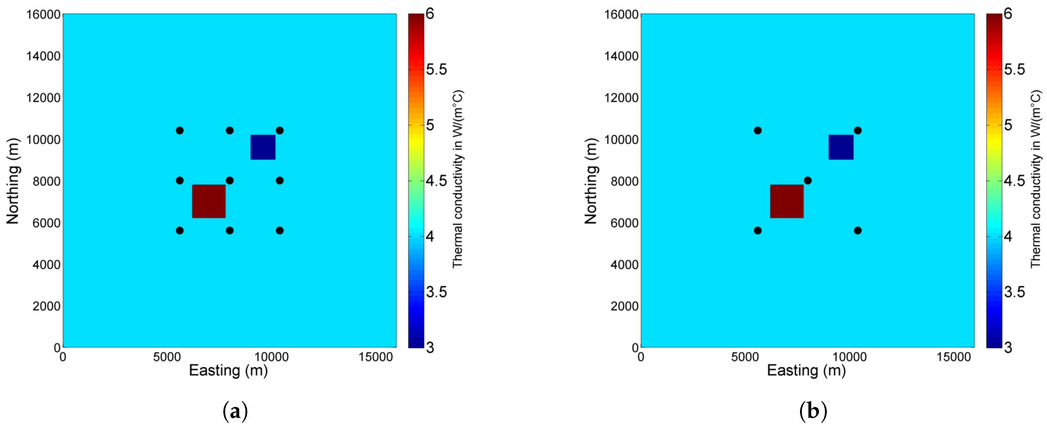
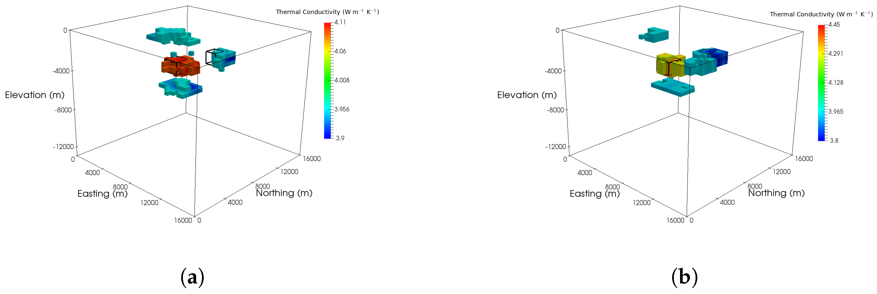
To demonstrate the capabilities of the inversion algorithms, we implemented them in MATLAB and inverted synthetic thermal data from two thermal models. By inverting these data, we explore the information content of thermal data in steady-state conductive settings. We also show examples of ways to incorporate prior information, such as expected thermal conductivity values or structural information. The techniques that we use to accommodate prior information shown in these examples are easy to implement. However, these inversion algorithms can also allow more advanced inversion tools to be applied to thermal data interpretation.

6.1. Block Model

We designed a simple thermal conductivity model consisting of two anomalous block bodies in a homogeneous background (Figure 2a). The southwestern anomalous body is 1.6 km on each side and 1.2 km deep, the top is 2.8 km deep and it has a conductivity of 6 W m−1 K−1. The northeastern body is 1.2 km on each side and 1.2 km deep, the top is 2 km deep and its conductivity is 3 W m−1 K−1. The background conductivity is 4 W m−1 K−1. We generated a three dimensional rectilinear mesh of 13,750 model cells including padding cells near the sides and the bottom of the mesh to reduce the effects of the boundary conditions on the computed fields near the anomalies. There are 25 layers of cells in each horizontal direction, organized as 5 padding layers, then 15 central layers, then 5 padding layers. Cells in the central region are cubes with sides of 400 m and padding layers are 1000 m long. Vertically from the surface down, there are 15 layers with depths of 400 m and then 7 padding layers with depths of 1000 m.
To produce synthetic thermal data, we simulated a geothermal gradient by enforcing a uniform vertical heat flow of 65 mW m−2 at the bottom of the mesh. We enforced a constant temperature of 20 °C at the top of the mesh and included no internal heat production.

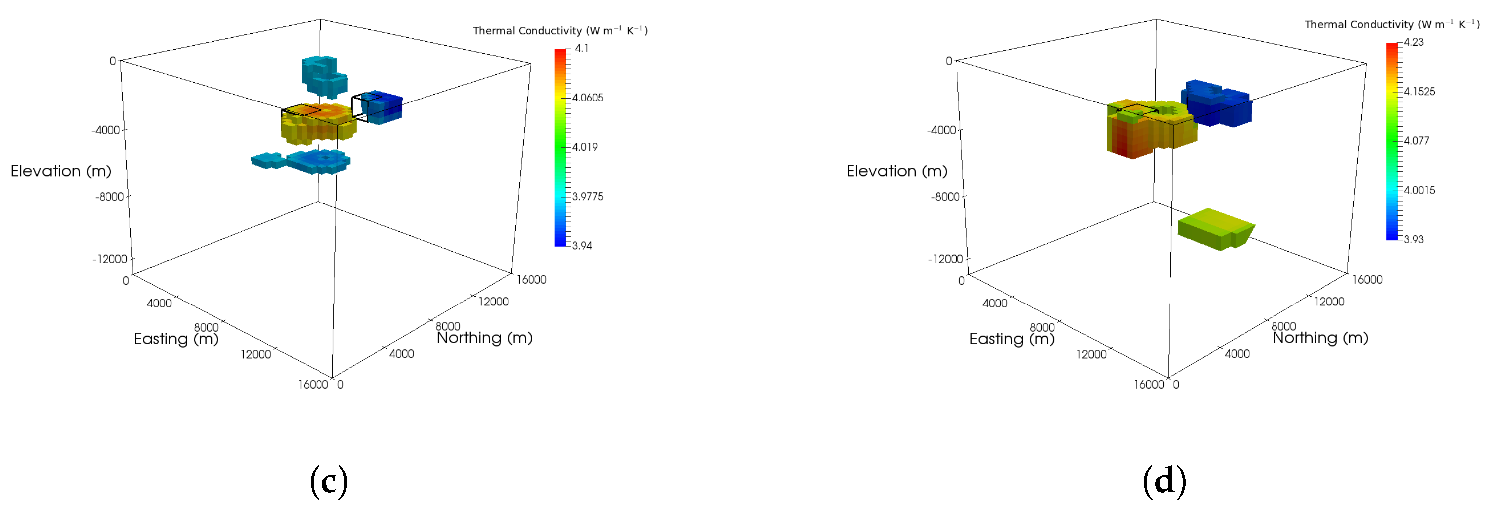
6.1.1. Surface Heat Flow Data Inversion

The block model was used to generate 169 synthetic surface heat flow data located in a 4.8 km by 4.8 km grid in the center of the model’s surface. The data are spaced 400 m in both northing and easting directions. We added Gaussian noise of mean zero and standard deviation 1.5 mW m−2 to the data. This configuration represents a more data-rich scenario rather than one commonly found in heat flow data and the noise level is low compared to common estimates of 5 per cent [30]. Furthermore, noise in heat flow data is rarely Gaussian. However, inverting this idealized synthetic data yields clearer insight into the inherent information content in heat flow data, which remains limited despite the data density and low Gaussian noise.
To illustrate the necessity of some form of weighting to counteract the decay of sensitivities, we first show a result of inverting surface heat flow data without imposing weighting, using p = 2 (Figure 2b). The largest deviations from background conductivity occur in the top layer of the recovered model and these deviations are not more than 0.01 W m−1 K−1. Clearly, if the model objective function is not weighted in some way, meaningful thermal conductivity structure is not recovered. When depth weighting is imposed, the tops of the resulting anomalies are located nearer to their true depths (Figure 2c). The anomalies themselves are smooth and spread out, due to the use of p = 2 in the model objective function. Note that the magnitudes of the recovered anomalies are still much closer to background than those of the true anomalies.
Using p = 1 , the recovered anomalies contrast more strongly with background (Figure 2d), as in the true model. Interestingly, the anomalies are adjacent to the sides of the model. This offset appears to be related to the depth of the anomalies. Additionally, the depths of the recovered anomalies are greater than the true depths. This result suggests that the depth weighting scheme warrants further investigation. Due to the non-linearity of the inverse problem, depth weighting may be less appropriate when anomalies with large conductivity contrasts are recovered. If that is the case, a model-dependent weighting scheme may be necessary. Alternatively, the sensitivities of model cells close to boundaries may not be compensated properly by the proposed depth weighting. To investigate this, we tried using sensitivity weighting computed from a homogeneous model, rather than depth weighting (Figure 2e). The resulting anomalies are closer to their true locations, vertically and horizontally, than the anomalies recovered using depth weighting, suggesting the possibility of a model-independent weighting scheme that compensates for sensitivity decay better than depth weighting.
These inversions demonstrate the sensitivity of heat flow data to thermal conductivity contrasts and the lack of depth information inherent in such data. They also show that the inversion algorithm can incorporate prior structural information via weighting functions and how the prior information can affect inversion results.

6.1.2. Borehole Temperature Data Inversion

Using the same thermal conductivity block model (Figure 2a), we simulated borehole temperatures in a nine-well configuration (Figure 3a) and a five-well configuration (Figure 3b). Temperature locations are evenly spaced down the wells every 100 m. Note that a precision temperature log would contain far smaller measurement spacing. However, since the mesh for this toy problem is coarse, little extra detail would be recovered in the inverted model by decreasing the spacing. Zero-mean random Gaussian noise with a standard deviation of 0.1 °C was added to the synthetic data. This noise level is above the precision of high quality thermisters but this amount of noise is lower than the noise encountered in precision temperature logs, which can be 0.5 °C [31]. As with the heat flow data example, we chose this low noise level to better understand the limits of the information content in borehole temperature data, regardless of noise level. We performed inversions using two different model norm measures: p = 2 and p = 1 . Sensitivity weighting was used for all inversions of borehole temperature data.
Using p = 2 for a nine-well configuration results in both positive and negative conductivity anomalies in the correct locations (Figure 4a). The anomalies’ conductivity values are much closer to that of the background than in the true model, though. Furthermore, false low conductivity anomalies appear above and below the positive block. These false “lobes” allow the model to fit the data while the conductivity of the positive block remains close to the background conductivity.
Using p = 1 , the anomalies remain in the same locations, and their conductivities are closer to their true values than the anomalies recovered using p = 2 (Figure 4b). The false “lobes” surround the positive block but not the negative block. Note that this block model, with its sharp conductivity contrasts and spatially compact anomalies, lends itself to an l 1 norm inversion.
For a five-well configuration, the anomalies tend to extend laterally into parts of the model where no data exists (Figure 4c,d). As with the nine-well configuration, using p = 1 (Figure 4d) results in anomalies whose conductivities deviate from background more than the anomalies in the p = 2 result (Figure 4c). However, they deviate less from background than the anomalies recovered from the nine-well configuration using p = 1 .
Unlike surface heat flow, borehole temperatures contain information about the depth extent of thermal conductivity anomalies, as seen in these results. We find that boreholes do not have to intersect thermal conductivity anomalies for those anomalies to be imaged by borehole temperature data. This is shown to be true for both the nine-well and five-well configurations.

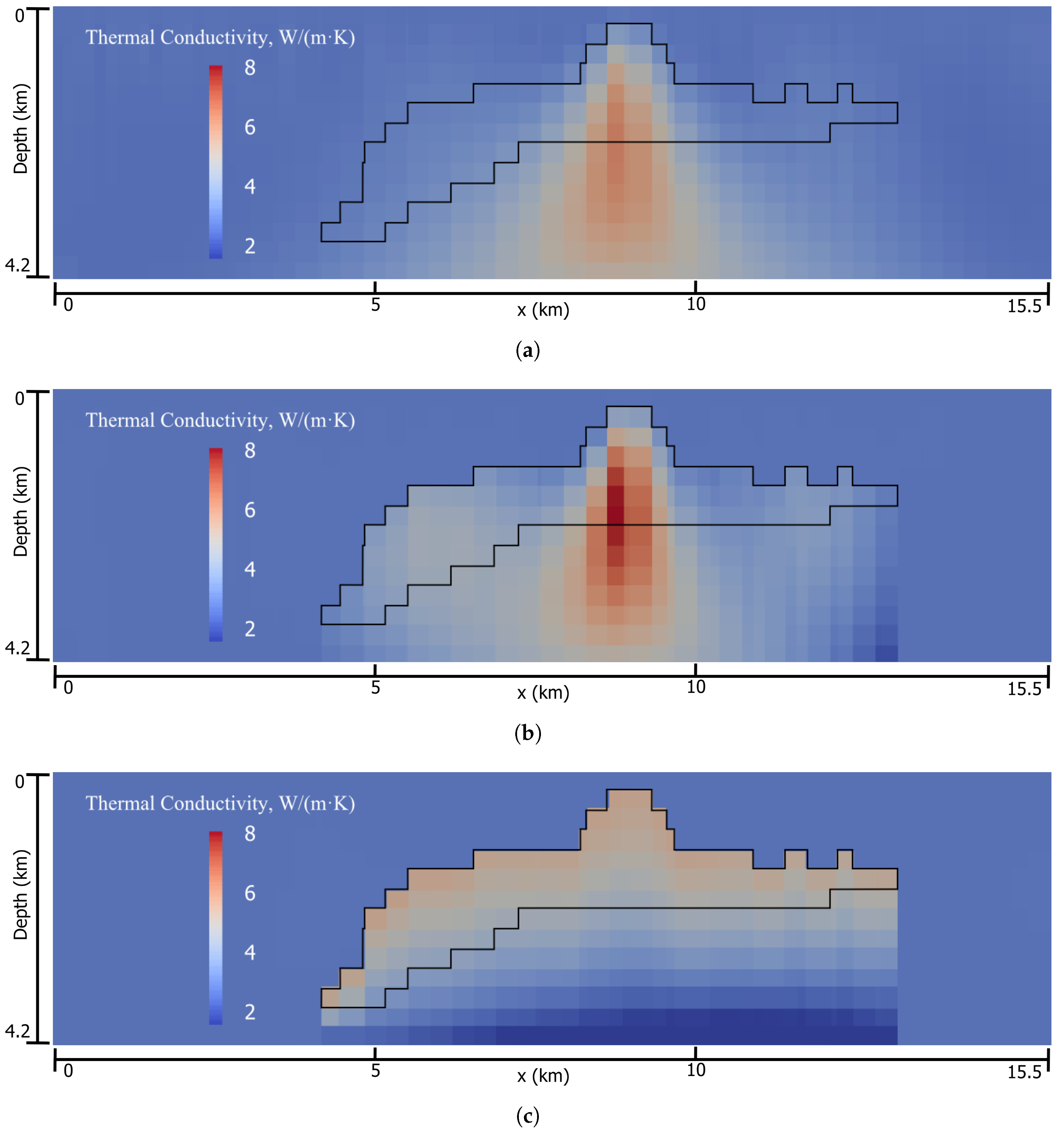
6.2. SEG/EAGE Salt Model

We now turn to a synthetic example of direct relevance in exploration problems. Imaging the base of salt remains a challenge in both exploration and tectonic studies in the salt provinces [32]. Gravity and magnetotelluric data have been used to aid in the seismic imaging of base of salt [33,34]. However, thermal data provides a unique complementary data set because of the high thermal conductivity contrast between salt and sediments [9]. Although exploring the joint use of thermal data with other geophysical data for this problem is beyond the scope of this paper, we explore the information content of thermal data through synthetic simulations.
Using the SEG/EAGE three dimensional salt model [35], we constructed a thermal conductivity model mimicking a salt body in a marine setting (Figure 5a). It is discretized into 63,525 rectilinear cells. The model spans 40.5 km in each horizontal direction and extends 11.2 km deep. The central 13.5 km by 13.5 km portion, in the top 4.2 km of the model, is where the salt body and the cross-sections shown in the figures are located (e.g., Figure 5b). Cells in this portion are cubes, 300 m to a side. Outside this volume are padding cells with horizontal lengths of 2.7 km and vertical thicknesses of 1 km. Each cell has been assigned either a thermal conductivity of 3 W m−1 K−1 if it corresponds to background sediments or 6 W m−1 K−1 if the cells is part of the salt body. A vertical heat flow of 95 mW m−2 was imposed at the bottom of the model, a constant temperature imposed at the top and no internal heat sources were included. A total of 225 synthetic heat flow data were generated in a grid over the body (Figure 5c). The data are located at the top of each column of model cells (at the sea floor) in the central portion of the model. Just as for the block model heat flow data, random zero mean Gaussian noise with a standard deviation of 1.5 mW m−2 was added to the data. Like with the block model, this scenario is idealized in terms of number of measurements and noise added in order to better understand the maximum information content that surface heat flow data can provide about subsurface thermal conductivity.
All inversions constrained the conductivities in padding cells to be that of background, implemented depth weighting and used p = 2 for the model objective function norm. The first inversion (Figure 6a) is otherwise unconstrained and uses a homogeneous reference model whose conductivity is that of background. The result is smooth and spread out. The top of the recovered model is close to the true depth to the top of the salt body, indicating that the depth weighting is appropriate for this inversion. Finer structural details of the salt body are not recovered. Seismic surveys can determine the geometry of the top of a salt body well. That structural information could be incorporated into a generalized inversion, as demonstrated by the result in Figure 6b. To obtain this result, we constrained all cells that lie above the salt body to have a conductivity equal to background. The recovered salt body honors the top structure but the conductivity values do not consistently match those of the true model and the bottom boundary is not well recovered. A reference model can incorporate prior knowledge of expected thermal conductivity values for different lithologies. In Figure 6c we demonstrate one way this can be accomplished. We construct a reference model based on the top surface of the salt body. In the reference model, the conductivity at the top of the salt is set to that of the salt. From there, the conductivity decreases linearly with depth to the bottom of the finely discretized region of the model. By using this reference model, we recover a model that more closely matches the true model and the bottom boundary of the salt body is better recovered.
These inversions results show that heat flow data contains information about the relative contrasts and spatial distribution of thermal conductivity in the subsurface. Both the horizontal extent and the depth to the top of an anomaly can be estimated from heat flow data, with only general prior information imposed in the form of depth weighting. The addition of other kinds of structural information can constrain relative thermal conductivities to be closer to the true values. Furthermore, incorporating prior information about both structure and expected conductivity values improves the imaging capability of the inversion algorithm.

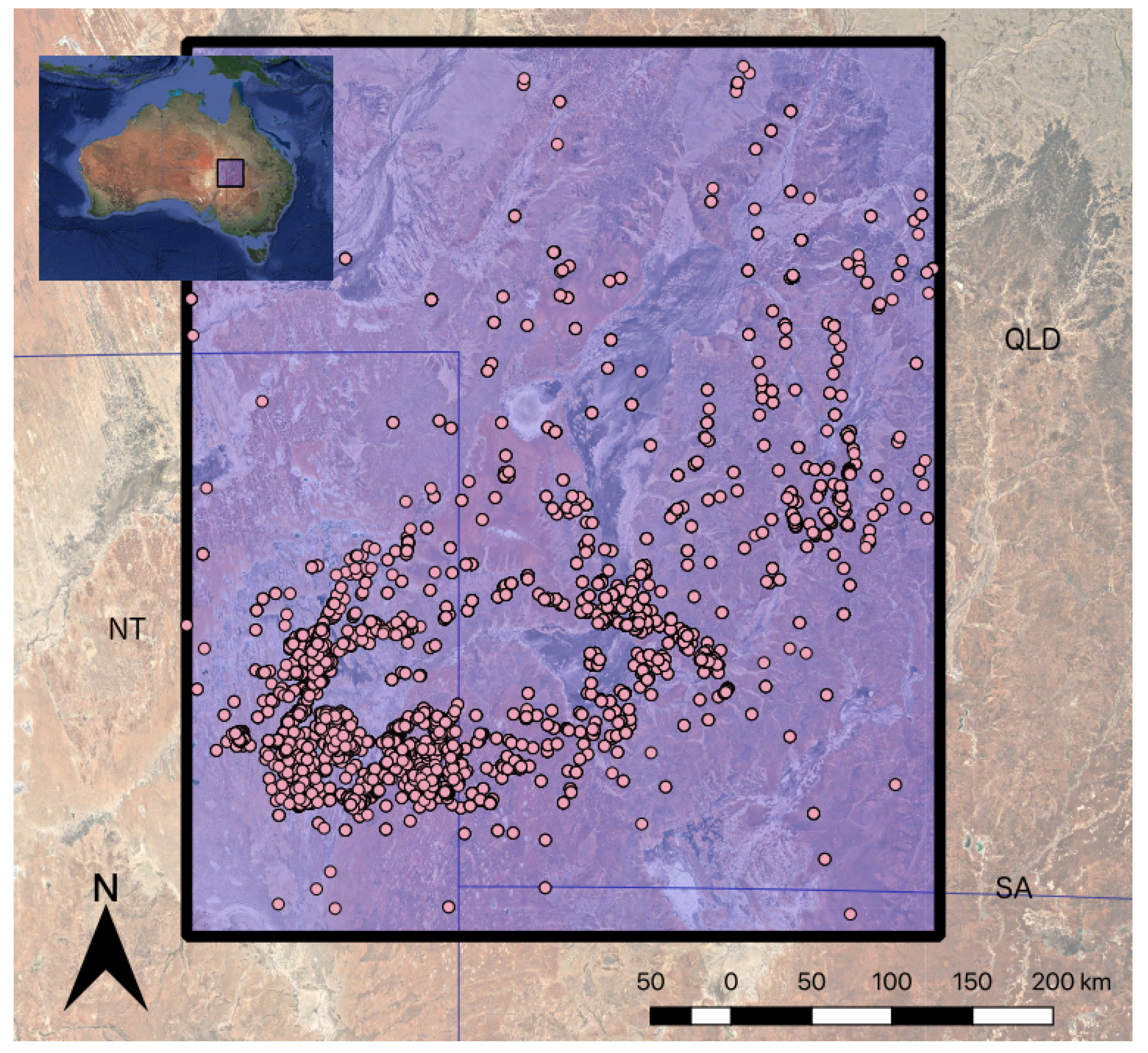
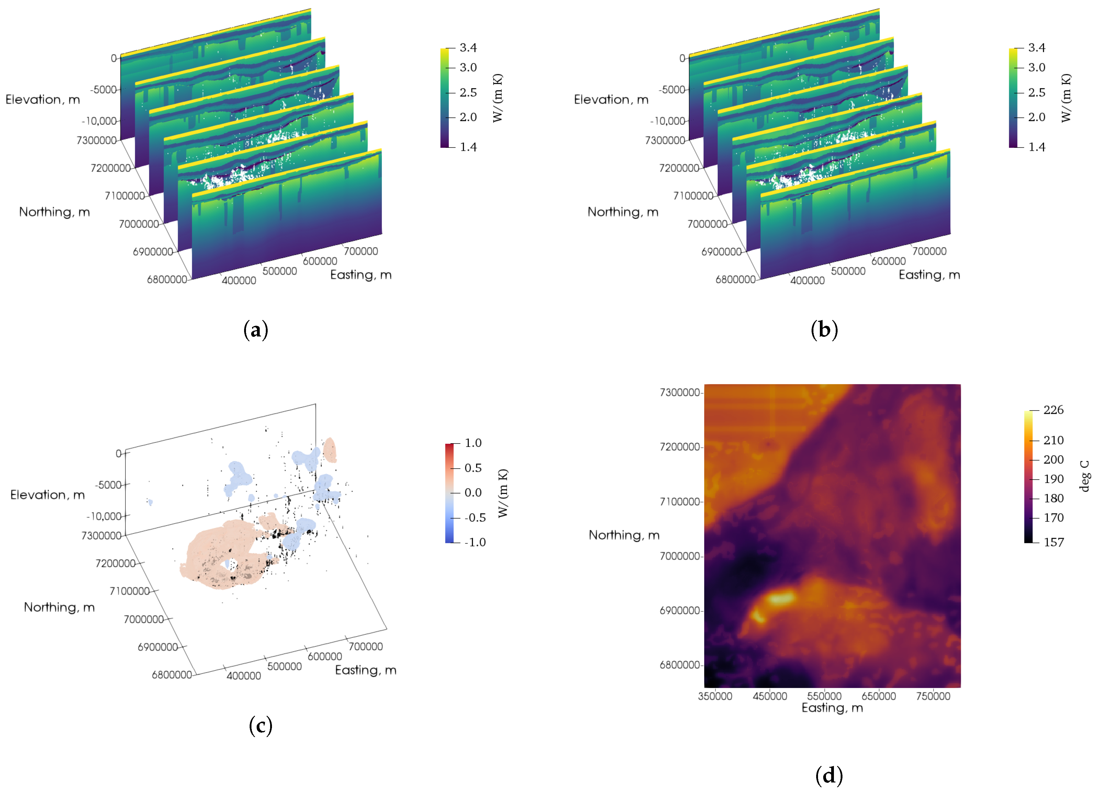
7. Inversions of Cooper Basin Data

To illustrate the utility of generalized inversion of temperature data, we inverted borehole temperature data from the Cooper Basin, a well-studied Australian geothermal prospect area. The Cooper Basin straddles the border between Queensland and South Australia. Oil and gas producers drilled the area extensively from the 1960s to the 1980s and amassed a large amount of borehole temperature data. The region contains unusually high heat flow which, in conjunction with thermally insulating sediments, results in anomalously high temperatures at 4–5 km depth. This attracted attention to the basin as a potential host for an enhanced geothermal system (EGS). Geoscience Australia organized the available thermal data and released it publicly [36]. Geoscience Australia also conducted an in-depth study of the area, generating a map of temperature at 5 km depth. This well-studied area provides an excellent opportunity to demonstrate the inversion methodology we have developed.
The basin was developed as an EGS by Geodynamics Limited from 2000 to 2015. Although the basin temperature was high enough, the deep hot granite at economic temperatures was too impermeable to circulate water at the rate needed for the resource to be economically viable [37]. The geothermal production wells were capped in 2016.
The OZTemp database contains temperature measurements from 5513 different wells located throughout Australia [36]. The data have been collected at various times using various instrumentation, so the data uncertainty is difficult to quantify. We identified 7481 temperature measurements from 1780 different boreholes in the Cooper Basin area to use in our inversion (Figure 7). We chose these data based on their location and their reliability, as indicated by flags in the OZTemp database. The trajectories of these wells are unknown, so we make the simplifying assumption that all wells are vertical.
In addition to publishing the thermal data, Geoscience Australia conducted an extensive study of the thermal regime of the region [38]. The authors of that study produce a geologic model and estimate heat production for each lithology in the model and the basal heat flow and surface temperature of the region. Here, we use these estimates as boundary conditions in the foward modeling process. Meixner et al. [38] also produce thermal conductivity estimates for each lithology in their geologic model. We compare our inversion results to that thermal conductivity model.

Field Data Inversions

We performed two inversions, which differ only in their reference models. For the Cooper Basin area, we assumed a constant surface temperature of 25 °C and impose known topography by setting the thermal conductivity of any cell above topography to 80 W m−1 K−1. The mesh and source distributions used for the inversions are the same as those published by Meixner et al. [38]. The mesh is a 234 by 277 by 137 rectilinear mesh that extends from 331000 E to 799000 E (GDA94/MGA zone 54), from 6761000 N to 7315000 N and from 600 m above sea level to 13,100 m below sea level. Every cell is 2000 m by 2000 m horizontally and 100 m deep. Basal heat flow is uniformly 48 mW m−2 and there is zero lateral heat flow through the sides of the model. Both inversions implemented distance weighting and used p = 2 for the model objective function norm. In the model objective function (Equation (30)), we used values of α s = 10 6 , α x = 400 , α y = 400 and α z = 0.25 , chosen based on the expected variation of thermal conductivity in the horizontal and vertical directions.
The first inversion used a reference model based on an assumption of a homogeneous conductivity, corrected for the effect of temperature on thermal conductivity (Figure 8a). This correction was carried out by first computing the temperature distribution resulting from a homogeneous thermal conductivity model of 3 W m−1 K−1. Next, the relationship between thermal conductivity and temperature used by Meixner et al. [38] was applied to correct the thermal conductivity values to reflect that temperature dependence. The Cooper Basin data were inverted, using that corrected thermal conductivity model as a reference model. The resulting inverted model (Figure 8b) is smooth, as expected. Structure in this model tends to be located near data observations. A large conductivity low can be seen in the 6900000 N cross-section which roughly corresponds to the Nappamerri Trough, where the highest temperatures at depth have been found. Low conductivity rock insulates the region below it from the surface, causing that region to be hotter than its surroundings. Figure 8c shows the regions of the model where the conductivity in the inversion results differs most from the reference model. The thermal conductivity of the inverted model is mostly lower than the reference model conductivity. Most changes between the reference model and the inverted model occur between the ground surface and 4000 m depth, which is generally the maximum depth of the temperature data. The largest changes are more than (1.0 W m−1 K−1). These appear in the eastern portion of the model. The resulting temperature distribution at 4 km below sea level is shown in Figure 8d. A temperature high can be seen in the southwestern part of the area, which is the region below the conductivity low. The high temperatures in the northern part of the model are suspect because there are few temperature data at depth in that area and the highest temperatures are close to the northern model boundary.
The second inversion uses the thermal conductivity model published by Meixner et al. [38] as a reference model (Figure 9a). This model was produced by first identifying boundaries for 16 lithologies from other geoscientific data, constructing a priori distributions for the thermal conductivity of each lithology and then stochastically inverting temperature data from the OZTemp database. Using their published model as a reference model, we performed a generalized inversion. The resulting inverted model is shown in Figure 9b. The structural boundaries in the reference model can be seen to be preserved in the inverted model. The change from the reference model is difficult to see but like the previous inversion result, it is most evident in the western portion of cross-section 6900000 N. A conductivity low appears in both inversion results. Figure 9d shows the temperature at 4 km below sea level for the second inversion. This result has a temperature maximum in the same southwestern area as in the previous result. This temperature high is not as pronounced as the one identified by Meixner et al. [38] but it is significant.
Comparing the results of the two inversions, similarities can be seen. The conductivity low that is common to the southwestern portion of both inversion results suggests that, presupposing that heat sources have been characterized accurately, such a feature does exist. Both inversions produce similar temperature maps at 4 km below sea level as well, both in terms of temperature range and spatial distribution. These similarities arise in part from the fact that both inversions use the same heat source distribution. However, their similarity lends confidence that this temperature distribution both agrees with the measured borehole temperatures and is relatively robust to variations in thermal conductivity. By the L-curve criterion, the inversions also provide estimates of the standard deviation of the data: 10.8 °C and 10.6 °C, respectively. Again, the similarity in the estimate lends credence to its accuracy.
Note that the results shown here are intended to illustrate the potential of the methodology. This is not a comprehensive examination of the temperature field of the Cooper Basin but rather a description of insights into its thermal characteristics that deterministic inversion offers.

8. Discussion

8.1. Information Content of Temperature Data

We have explored the information about thermal conductivity contained in borehole temperature data by inverting different configurations of data locations. Inversion results suggest that the inherent depth resolution of borehole temperature data is the maximum depth of the data, although it may be possible to resolve anomalies deeper than the deepest measurement by incorporating prior structural information. Contrasting horizontal layers can be recovered if temperature data exists in holes that penetrate the layers. Data in boreholes that do not intersect bodies of anomalous thermal conductivity can be used to detect the bodies but the geometry of the bodies is better resolved by data in boreholes that intersect the anomalous bodies.
The choice of vertical heat flow values imposed at the bottom boundary of the model affects the result recovered by inverting borehole temperatures. For instance, if the bottom heat flow values are halved, the recovered conductivity model will also be halved, which follows intuitively from Equation (4). Thus, there is an inherent ambiguity between the absolute thermal conductivity and the vertical heat flow which temperature measurements alone cannot resolve. Thermal conductivity measurements or estimates must be leveraged in order to resolve the ambiguity.

8.2. Information Content of Heat Flow Data

Surface heat flow data are sensitive to horizontal variations in thermal conductivity beneath the measurement locations. However, because heat flow is dominantly vertical, the data have low lateral sensitivity. Furthermore, like gravity and magnetic data, surface heat flow data contain no inherent depth information. Therefore, surface heat flow data are unable to distinguish a horizontally layered conductivity model from a homogeneous half-space. Only with the addition of prior information can subsurface structures be resolved.
In addition, surface heat flow data are only sensitive to relative changes in thermal conductivity. For example, if all the thermal conductivity values in a model are doubled, the surface heat flow distribution will remain unaffected. Speaking practically, heat flow measurements require a direct measurement of the thermal conductivity, so this does not apply at the measurement location. Below the measurement location, though, absolute thermal conductivity cannot be determined from surface heat flow.
This follows intuitively from the concept of heat conservation: if a certain heat flow is imposed at the bottom of a region and not allowed to escape through the sides, then that amount of heat must flow up through the region and exit through the surface at the top of the region, regardless of how conductive that region is. By this same logic, surface heat flow measurements can be used to validate the choice of heat flow imposed at the bottom of the model (the non-zero Neumann boundary condition).

8.3. Practical Considerations and Assumptions

Several simplifying assumptions must be sufficiently valid in order to apply these inversion methods. First, the area must be nearly in thermal steady-state. Therefore, effect of ground surface temperature changes must be negligible. This means in part that the paleoclimate effect must be negligible in the area or the effect must be removed from the data. Additionally, the region must be tectonically stable. Second, heat flow must be dominantly conductive, meaning that the effects of subsurface water flow or other forms of convection on the subsurface temperature field must be negligible. Third, the anomalous thermal conductivities must lie within the model domain, far enough away from the edges of the model such that a negligible amount of heat flows laterally into or out of the model. Additionally, the boundary conditions must be sufficiently accurate. This means that the temperatures of the surface of the earth must be known or estimated, as well as the basal heat flow. It also means that the sides of the model must be sufficiently far away from the data that the assumption of vertical heat flow at the sides does not significantly affect the predicted data.
Generally, the thermal conductivity of the subsurface depends on temperature. One approach to accounting for the dependence is to include it in the forward modeling process. Such an approach usually involves an iterative process, alternating between computing temperatures and adjusting thermal conductivities based on those computed temperatures. In this study, though, we did not include temperature dependence during inversions. As formulated above, the inversion algorithms recover true thermal conductivity, meaning the thermal conductivity as it is at subsurface temperatures. Therefore, temperature dependence does not necessarily need to be included in the forward modeling operation. However, the algorithm also regularizes the true thermal conductivity. This may not be desirable since the thermal conductivity of a single rock type is expected to vary with temperature and should not be penalized for that variance. To address this problem during the Cooper Basin inversions, we used reference models that incorporate the temperature dependence of thermal conductivity. Deviations from the reference model are penalized, so the reference model implicitly enforced the temperature dependence.
This approach is adequate as long as the differences between temperatures computed from the reference model and temperatures computed from the inverted model are small enough to neglect the accompanying change in thermal conductivity due to temperature dependence. Otherwise, the reference model can be updated to account for them as follows. After each Gauss-Newton step, a predicted temperature field is produced. This temperature field can be used to compute a temperature-corrected reference model from the original uncorrected reference model. The new corrected model can then be used as a reference model in the next Gauss-Newton step. This process can be continued until convergence criteria are satisfied and the inversion is stopped.
We also remark that these methods do not account for anisotropic thermal conductivity. The ambiguity of thermal data is such that it would be difficult to deduce anisotropy from temperature and heat flow data alone. However, if information about anisotropy is known in advance, the forward and inverse algorithms can be modified to incorporate it.

9. Conclusions

We have developed inverse methods to recover three-dimensional thermal conductivity distributions from thermal data in a steady-state conductive setting. We used the methods to quantitatively analyze the effects of thermal conductivity contrasts on surface heat flow and subsurface temperatures and to better understand how thermal data constrains the space of possible thermal models. We showed that techniques such as l p norm inversion and sensitivity weighting, which allow a priori information to be incorporated into generalized inversions, can be implemented to improve the interpretation of thermal data.
A wide range of generalized inversion tools can be applied to thermal data via these methods. In addition, generalized inversions for other physical quantities besides thermal conductivity can be developed by following this methodology. These methods can also be used to interpolate temperatures or heat flows based on a physically plausible thermal model or to assess the possibility that observed thermal data can explained by variations in thermal conductivity alone.
Furthermore, this work paves the way for generalized joint inversions that incorporate thermal data with other kinds of geophysical data. Thermal data are especially amenable to joint inversion because they can be linked with many physical phenomena. For example, electrical conductivity is often temperature dependent. Also, groundwater flow affects the temperature field, so data that is sensitive to groundwater is a good candidate for joint or coupled inversion with thermal data. We hope that this work advances such multiphysics-based interpretations.

Author Contributions

Conceptualization, W.A.M. and Y.L.; methodology, W.A.M. and Y.L.; software, W.A.M.; validation, W.A.M.; formal analysis, W.A.M.; investigation, W.A.M.; resources, W.A.M and Y.L.; data curation, W.A.M.; writing—original draft preparation, W.A.M.; writing—review and editing, W.A.M. and Y.L.; visualization, W.A.M.; supervision, Y.L.; project administration, Y.L.; funding acquisition, Y.L.

Funding

This work was funded by a fellowship from the Apache Corporation, a scholarship from the Hess Corporation and the “Gravity and Magnetics Research Consortium” (GMRC) at the Colorado School of Mines. The sponsoring companies at the time of work are Anadarko, Bell Geospace, BG Group, BGP International, CGG, Lockheed Martin, Marathon Oil, Micro-g LaCoste, Petrobras, Shell, Tullow Oil and Vale.

Acknowledgments

Cooper Basin temperature data comes from the OZTemp database, copyright Commonwealth of Australia (Geoscience Australia) 2010. We thank Paul Morgan and David Walraven for sharing their valuable insights.

Conflicts of Interest

The authors declare no conflict of interest. The funders had no role in the design of the study; in the collection, analyses or interpretation of data; in the writing of the manuscript, or in the decision to publish the results.

Appendix A. Matrix Definitions

Appendix A.1. The Gradient Operator

The discrete gradient operator G can be formed as
G = A s G l .
Here A s is a n f × n f diagonal matrix whose diagonal elements are cell face areas, where n f is the total number of cell faces. The diagonal entries of A s are ordered such that faces with normal vectors in the x direction are first, followed by those in the y direction, and finally those in the z direction. The entries with the same normal vary fastest in the z direction and slowest in the x direction. G l is a n f × n v logical gradient operator matrix, where n v is the number of control volumes, or cells. Its entries are −1, 1, and 0. For a rectilinear mesh,
G l = G lx G ly G lz ,
G l = G lx G ly G lz T ,
where G lx can be expressed as
G lx = G ˜ lx I n y I n z ,
where ⊗ denotes a Kronecker product. G ˜ lx takes the form of an n x × n x + 1 matrix,
G ˜ lx = 1 1 1 1 1 1 .
G ly and G lz are similarly constructed:
G ly = I n x G ˜ ly I n lz G lz = I n x I n ly G ˜ lz
where G ˜ ly and G ˜ lz have the same form as G ˜ lx in their respective directions. Note that this form of the gradient operation has units of distance squared. A true gradient operator with units of one over distance could be constructed as G i = diag A v V 1 A s G l , where V is an n v × 1 vector whose entries are cell volumes, and A v is an n f × n v averaging matrix, described in detail in the next section.

Appendix A.2. The Harmonic Interpolant

The matrix M is an n f × n f diagonal matrix whose elements are related to harmonically averaged thermal conductivities. It can be expressed as
M = B diag A v V σ 1 1 .
Here, B is an n f × n f diagonal matrix which allows Neumann boundary conditions to be incorporated. It is a modified identity matrix, with entries set to zero if they correspond to faces where Neumann boundary conditions are enforced. A v is an n f × n v averaging matrix. Its purpose is to interpolate conductivities from cell centers to cell faces arithmetically, as a step in harmonic averaging. For a rectilinear grid,
A v = A vx A vy A vz T ,
where A vx can be expressed as
A vx = A ˜ vx I n y I n z .
A ˜ vx takes the form of an n x × n x + 1 matrix,
A ˜ vx = 1 2 1 2 1 2 1 2 1 2 1 2 .
A vy and A vz are similarly constructed:
A vy = I n x A ˜ vy I n vz A vz = I n x I n vy A ˜ vz .
V is an n v × n v diagonal matrix whose entries are cell volumes. σ is an n v × 1 column vector of conductivities at cell centers, and σ 1 denotes an element-wise inverse of σ (raising each element of σ to the power of 1 ).

Appendix A.3. The Full Forward Operation

The forward operation can be expressed as solving the linear system
Au = b .
Here, A is a n v × n v symmetric coefficient matrix, where
A = G T MG .
b is a n v × 1 right-hand vector, where
b = Vf G T MG BC u BC + G T q BC .
Here V is a diagonal matrix of cell volumes as defined above. f is a n v × 1 column vector of source terms with units of power per unit volume. G BC can be expressed as
G BC = A s G BCl ,
where A s is a diagonal matrix of cell face areas as defined above, and G BCl is an n f × n f modified identity matrix. For faces that bound the volume of interest, if the normal to the face that points outward from the volume of interest points in the positive x, y, or z direction, then the corresponding diagonal entry of G BCl is 1. If the normal points in the negative x, y, or z direction, then the corresponding entry is 1 . u BC is an n f × 1 column matrix of known Dirichlet boundary conditions (temperatures) at cell faces, with zero values at faces where no Dirichlet boundary condition is imposed. Similarly, q BC is an n f × 1 column matrix of known Neumann boundary conditions (heat flows) at cell faces, with zero values at faces where no Neumann boundary condition is imposed.

Appendix A.4. Interpolation

The temperature and heat flow fields are computed at cell centers and cell faces, respectively. Data can be located anywhere, though, so it is necessary to interpolate from the computed fields to data locations. We construct a matrix Q u to interpolate temperatures, and a matrix Q q to interpolate heat flows. Both matrices implement trilinear interpolation. Thus, temperature data can be expressed as
d u = Q u u ,
and heat flow data as
d q = Q q q .

Appendix B. Sensitivity Derivation and Computation

The following is a derivation of the sensitivities of temperature and heat flow to thermal conductivity, and an explanation of how this result can be used without explicitly forming the sensitivity matrix. These derivations follow methods laid out by Oliver et al. [11] and Haber [39]. We begin with an equation of the form
c ( m , s ) = 0
where m is a spatially varying model parameter vector and s is a vector of values of a field that depends on m . It follows that
m c ( m , s ) δ m + s c ( m , s ) δ s = 0 .
The sensitivity matrix is
J = d m = m d ,
where d is a vector of measurements of the field s . If we define a matrix Q that interpolates from the field s to the data d such that
Qs = d ,
then J can be expressed as
J = Q s m = Q m s .
From Equation (A19), it can be shown that the sensitivity matrix expressed in terms of c ( m , d ) is
J = Q s c 1 m c .

Appendix B.1. Temperature Sensitivity

We can write
Au b = 0 .
This equation is of the form
c u ( σ , u ) = 0 ,
where there exists forward and inverse mappings from m to the conductivity σ . Note that we can apply the chain rule to Equation (A23) to obtain
J = Q u u c u 1 σ c u m σ .
So, to find the sensitivity matrix, we need expressions for u c u and σ c u . First,
u c u = A .
Next,
σ c u = σ G T M G u + G BC u BC G T q BC Vf = G T σ M G u + G BC u BC = G T K ,
where K = σ M G u + G BC u BC . We define K because we will use this result several times. Let us now evaluate K :
K = σ M G u + G BC u BC = σ B diag A v V σ 1 1 G u + G BC u BC = B diag Gu + G BC u BC σ A v V σ 1 1 .
Next, we can use the chain rule and the vector calculus identity
x y 1 = diag y 2 x y
to evaluate the derivative, yielding
K = B diag Gu + G BC u BC × diag A v V σ 1 2 A v V diag σ 2 ,
Let us define H = σ c u = G T K . Then, the sensitivity matrix for temperature data is
J u = Q u A 1 H m σ .
If m = σ , then this equation simplifies to
J u = Q u A 1 H .
Alternatively, if m = ln σ , then the equation simplifies to
J u = Q u A 1 H diag σ .

Appendix B.2. Heat Flow Sensitivity

From Equations (18) and (22), we obtain
q q BC + MGu + MG BC u BC = 0 ,
where u = A 1 b is a function of σ . Thus, Equation (A35) is of the form
c q ( σ , q ) = 0 ,
so the sensitivity matrix can be expressed as
J q = Q q ( q c q ) 1 σ c q ,
where Q q is an interpolation matrix for heat flow data. From Equation (A35) it is clear that
( q c q ) 1 = I n f .
So, it remains to find σ c q . We can do so by applying the following version of the product rule:
x Ay = x A y + A x y ,
where the term x A y is equivalent to evaluating x Ay as if y were independent of x . Thus,
σ c q = σ M Gu + G BC u BC + M σ Gu + G BC u BC .
Since evaluating the first term in the above expression is equivalent to evaluating σ M Gu + G BC u BC as if u were independent of σ , we can apply Equation (A29) to yield
σ M Gu + G BC u BC = K .
The second term can be expressed as
M σ Gu + G BC u BC = MG σ u .
Note that the sensitivity matrix J u derived in Equation (A32) can be expressed as
J u = Q u σ u m σ .
Thus,
σ u = A 1 H ,
and
σ c q = K MGA 1 H .
So, the heat flow sensitivity matrix is
J q = Q q K MGA 1 H m σ .
Again, if m = σ , then the equation simplifies to
J q = Q q K MGA 1 H ,
whereas if m = ln σ , then the equation simplifies to
J q = Q q K MGA 1 H diag σ .

Appendix B.3. Computing Sensitivity Vector Products

For each Gauss-Newton step, a linear system of equations must be solved. That system can be solved by a conjugate gradient method, which only requires an algorithm to calculate products of a vector with the sensitivity matrix, J , and with its transpose, J T . The sensitivity matrix itself is not required. If m = σ , those matrix vector products can be computed as follows.
  • Temperature: Compute x = J u v
    • Compute y = Hv .
    • Solve Az = y for z .
    • Compute x = Q u z .
  • Temperature: Compute x = J u T v
    • Compute y = Q u T v .
    • Solve A T z = y for z (equivalently, solve Az = y since A is symmetric).
    • Compute x = Hz .
  • Heat flow: Compute x = J q v
    • Compute y = Hv .
    • Solve Az = y for z .
    • Compute x = Q q Kv MGz .
  • Heat flow: Compute x = J q T v
    • Compute w = Q q T v .
    • Compute y = G T Mw .
    • Solve A T z = y for z .
    • Compute x = K T w + H T z .

References

  1. Beardsmore, G.R.; Cull, J.P. Crustal Heat Flow: A Guide to Measurement and Modelling; Cambridge University Press: Cambridge, UK, 2001. [Google Scholar]
  2. Stein, C.A.; Stein, S. A model for the global variation in oceanic depth and heat flow with lithospheric age. Nature 1992, 359, 123–129. [Google Scholar] [CrossRef]
  3. Mottaghy, D.; Pechnig, R.; Vogt, C. The geothermal project Den Haag: 3D numerical models for temperature prediction and reservoir simulation. Geothermics 2011, 40, 199–210. [Google Scholar] [CrossRef]
  4. Anderson, M.P. Heat as a ground water tracer. Groundwater 2005, 43, 951–968. [Google Scholar] [CrossRef] [PubMed]
  5. Wang, K.; Beck, A. An inverse approach to heat flow study in hydrologically active areas. Geophys. J. Int. 1989, 98, 69–84. [Google Scholar] [CrossRef] [Green Version]
  6. Jokinen, J.; Kukkonen, I.T. Inverse simulation of the lithospheric thermal regime using the Monte Carlo method. Tectonophysics 1999, 306, 293–310. [Google Scholar] [CrossRef]
  7. Rath, V.; Wolf, A.; Bücker, H. Joint three-dimensional inversion of coupled groundwater flow and heat transfer based on automatic differentiation: Sensitivity calculation, verification, and synthetic examples. Geophys. J. Int. 2006, 167, 453–466. [Google Scholar] [CrossRef]
  8. Jardani, A.; Revil, A. Stochastic joint inversion of temperature and self-potential data. Geophys. J. Int. 2009, 179, 640–654. [Google Scholar] [CrossRef] [Green Version]
  9. Nagihara, S. Three-dimensional inverse modeling of the refractive heat-flow anomaly associated with salt diapirism. AAPG Bull. 2003, 87, 1207–1222. [Google Scholar] [CrossRef]
  10. Papadopoulos, D.; Herty, M.; Rath, V.; Behr, M. Identification of uncertainties in the shape of geophysical objects with level sets and the adjoint method. Comput. Geosci. 2011, 15, 737–753. [Google Scholar] [CrossRef]
  11. Oliver, D.S.; Reynolds, A.C.; Liu, N. Inverse Theory for Petroleum Reservoir Characterization and History Matching; Cambridge University Press: Cambridge, UK, 2008. [Google Scholar]
  12. Shen, P.Y.; Beck, A. Least squares inversion of borehole temperature measurements in functional space. J. Geophys. Res. Solid Earth 1991, 96, 19965–19979. [Google Scholar] [CrossRef]
  13. Ollinger, D.; Baujard, C.; Kohl, T.; Moeck, I. Distribution of thermal conductivities in the Groß Schönebeck (Germany) test site based on 3D inversion of deep borehole data. Geothermics 2010, 39, 46–58. [Google Scholar] [CrossRef]
  14. Hermanrud, C.; Cao, S.; Lerche, I. Estimates of virgin rock temperature derived from BHT measurements: Bias and error. Geophysics 1990, 55, 924–931. [Google Scholar] [CrossRef]
  15. Andaverde, J.; Verma, S.P.; Santoyo, E. Uncertainty estimates of static formation temperatures in boreholes and evaluation of regression models. Geophys. J. Int. 2005, 160, 1112–1122. [Google Scholar] [CrossRef] [Green Version]
  16. Goutorbe, B.; Lucazeau, F.; Bonneville, A. Comparison of several BHT correction methods: A case study on an Australian data set. Geophys. J. Int. 2007, 170, 913–922. [Google Scholar] [CrossRef]
  17. Nagihara, S.; Christie, C.H.; Richards, M. Comparison of Methodologies for Correcting Bottom-Hole Temperature Measurements: An Example from the East Cameron and West Cameron Federal Lease Areas in the Gulf of Mexico. Gulf Coast Assoc. Geol. Soc. Trans. 2014, 64, 293–302. [Google Scholar]
  18. Stuwe, K. Energetics: Heat and Temperature. In Geodynamics of the Lithosphere: An Introduction; Springer: Berlin/Heidelberg, Germany, 2007; pp. 51–137. [Google Scholar] [CrossRef]
  19. Eymard, R.; Gallouët, T.; Herbin, R. Finite volume methods. Handb. Numer. Anal. 2000, 7, 713–1018. [Google Scholar] [Green Version]
  20. Hyman, J.M.; Knapp, R.J.; Scovel, J.C. High order finite volume approximations of differential operators on nonuniform grids. Phys. D Nonlinear Phenom. 1992, 60, 112–138. [Google Scholar] [CrossRef]
  21. Golub, G.H.; Van Loan, C.F. Matrix Computations; John Hopkins University Press: Baltimore, MD, USA, 2012; Volume 3. [Google Scholar]
  22. Forsyth, P.; Sammon, P. Quadratic convergence for cell-centered grids. Appl. Numer. Math. 1988, 4, 377–394. [Google Scholar] [CrossRef]
  23. Farquharson, C.G.; Oldenburg, D.W. Non-linear inversion using general measures of data misfit and model structure. Geophys. J. Int. 1998, 134, 213–227. [Google Scholar] [CrossRef] [Green Version]
  24. Hansen, P.C. The L-Curve and its Use in the Numerical Treatment of Inverse Problems. In Computational Inverse Problems in Electrocardiology; Johnston, P., Ed.; WIT Press: Southampton, UK, 2001. [Google Scholar]
  25. Vogel, C.R. Computational Methods for Inverse Problems; Society of Industrial and Applied Mathematics, Frontiers in Applied Mathematics: Philadelphia, PA, USA, 2002; Volume 23. [Google Scholar]
  26. Nocedal, J.; Wright, S.J. Numerical Optimization, 2nd ed.; Springer Series in Operations Research; Springer: New York, NY, USA, 1999. [Google Scholar]
  27. Li, Y.; Oldenburg, D.W. Joint inversion of surface and three-component borehole magnetic data. Geophysics 2000, 65, 540–552. [Google Scholar] [CrossRef]
  28. Portniaguine, O.; Zhdanov, M.S. 3-D magnetic inversion with data compression and image focusing. Geophysics 2002, 67, 1532–1541. [Google Scholar] [CrossRef]
  29. Li, Y.; Oldenburg, D.W. 3-D inversion of gravity data. Geophysics 1998, 63, 109–119. [Google Scholar] [CrossRef]
  30. Hyndman, R.D.; Davis, E.E.; Wright, J.A. The measurement of marine geothermal heat flow by a multipenetration probe with digital acoustic telemetry and insitu thermal conductivity. Mar. Geophys. Res. 1979, 4, 181–205. [Google Scholar] [CrossRef]
  31. Houseman, G.A.; Cull, J.P.; Muir, P.M.; Paterson, H.L. Geothermal signatures and uranium ore deposits on the Stuart Shelf of South Australia. Geophysics 1989, 54, 158–170. [Google Scholar] [CrossRef]
  32. Jones, I.F.; Davison, I. Seismic imaging in and around salt bodies. Interpretation 2014, 2, SL1–SL20. [Google Scholar] [CrossRef] [Green Version]
  33. Routh, P.S.; Jorgensen, G.J.; Kisabeth, J.L. Base of the salt imaging using gravity and tensor gravity data. In SEG Technical Program Expanded Abstracts 2001; Society of Exploration Geophysicists: Tulsa, OK, USA, 2001; pp. 1482–1484. [Google Scholar]
  34. Hoversten, G.M.; Constable, S.C.; Morrison, H.F. Marine magnetotellurics for base-of-salt mapping: Gulf of Mexico field test at the Gemini structure. Geophysics 2000, 65, 1476–1488. [Google Scholar] [CrossRef]
  35. Aminzadeh, F.; Brac, J.; Kunz, T. 3-D Salt and Overthrust Models; Society of Exploration Geophysicists: Tulsa, OK, USA, 1997. [Google Scholar]
  36. Holgate, F.; Gerner, E. OZTemp Well Temperature Data; Geoscience Australia: Canberra, Australia, 2010. [Google Scholar]
  37. Holl, H.G. What Did We Learn about EGS in the Cooper Basin? Geodynamics Limited: Milton, Australia, 2015. [Google Scholar]
  38. Meixner, A.; Kirkby, A.; Lescinsky, D.; Horspool, N. The Cooper Basin 3D Map Version 2: Thermal Modelling and Temperature Uncertainty; Geoscience Australia: Canberra, Australia, 2012; Volume 60. [Google Scholar]
  39. Haber, E. Computational Methods in Geophysical Electromagnetics; Society for Industrial and Applied Mathematics: Philadelphia, PA, USA, 2014. [Google Scholar]
Figure 1. (a) Sensitivity of one borehole temperature datum to thermal conductivity for a homogeneous thermal conductivity model. The temperature datum is located in the center of the cell marked by the X. Temperature increases at that location if the thermal conductivity of red cells increases. Temperature decreases with an increase in the thermal conductivity of blue cells. The sensitivity decays with distance from the location of the temperature datum, especially laterally. (b) The decay of the sensitivity of surface heat flow to thermal conductivity as a function of the depth of the conductivity. The sensitivities were computed on a 50 by 50 by 50 regular grid for a homogeneous thermal conductivity model. A decay rate proportional to z 3 is overlain on the plot. The fit serves to justify the use of the proposed depth weighting function.
Geosciences 09 00293 g001
Figure 2. Inversions of synthetic surface heat flow data. (a) Block model of thermal conductivity, used to generate the synthetic data. The southwestern anomaly has a conductivity of 6 W m−1 K−1, the northeastern anomaly has a conductivity of 3 W m−1 K−1 and the background conductivity is 4 W m−1 K−1. (b) Inversion result using an l p norm for the model objective function, with p = 2 and no weighting. The recovered conductivity anomalies are all near the surface, demonstrating the need to weight the model objective function. (c) Inversion result with p = 2 and depth weighting. Two anomalous zones are imaged but the depth extent is not well-defined and the conductivities of the anomalies are close to the background conductivity. (d) Inversion result with p = 1 and depth weighting. The anomalies are located near at the bottom of the model, against the northern and southern sides. The conductivities of the anomalies are close to the conductivities in the true model. (e) Inversion result with p = 1 and sensitivity weighting. The depths to the tops of the recovered anomalies are greater than the true anomalies’ depths and their depth extent is greater. The conductivities of the anomalies are close to background conductivity.
Geosciences 09 00293 g002
Figure 3. Plan views of borehole locations and thermal conductivity anomalies used for inversions of sythetic borehole temperature data, for (a) a nine-well configuration and (b) a five-well configuration.
Geosciences 09 00293 g003
Figure 4. (a) Inversion result for borehole temperature data in the nine-well configuration with p = 2. Anomalous zones of conductivity are located near the true anomalies. Additional low conductivity “lobes” are located above and below the positive anomaly. The recovered conductivities are close to the background conductivity. (b) Inversion result for borehole temperature data in the nine-well configuration with p = 1. Compared to the p = 2 result, the false “lobes” are less pronounced and the conductivity values contrast more strongly with background. (c) Inversion result for five-well configuration with p = 2. Compared to the nine-well results, the anomalies are less well-defined horizontally and they contrast less with the background. (d) Inversion result for borehole temperature data in the five-well configuration with p = 1. Like the nine-well results, the “lobes” are less pronounced in the p = 1 result than in the p = 2 result and the conductivity contrast is greater. The anomalies are less well-defined horizontally for the five-well configuration, though.
Geosciences 09 00293 g004aGeosciences 09 00293 g004b
Figure 5. (a) A thermal conductivity model constructed from the SEG/EAGE salt model [35]. The blue plane shows the location of the cross-sections shown below. (b) A cross-section of the model in (a). (c) Synthetic heat flow data generated using the model, without noise, demonstrating the effect of the salt body on surface heat flow.
Geosciences 09 00293 g005
Figure 6. (a) Cross-section, excluding padding cells, of an inversion result constraining only padding cells. The depth to the top of the anomaly and the maximum thermal conductivity are similar to the true model but the structure of the salt body is not well-defined. (b) Cross-section, excluding padding cells, of the result of inversion constraining all cells above and outside the salt body. The horizontal extent of the body is better defined and the maximum conductivity value is higher than in the true model. The base of the salt is still not defined. (c) Cross-section, excluding padding cells, of an inversion result using a reference model built from the top of the salt. By incorporating the expected value of the conductivity of the salt body into the reference model, the base of the salt body is better recovered.
Geosciences 09 00293 g006
Figure 7. Cooper Basin temperature well locations, with the horizontal extent of the thermal model shaded blue.
Geosciences 09 00293 g007
Figure 8. (a) Cross-sections of a reference thermal conductivity model built from a homogeneous lithology model, with a vertical exaggeration factor of 20. The model incorporates the temperature dependence of thermal conductivity. Data locations are shown in white. (b) Cross-sections of an inversion of OZTemp borehole temperature data using the model in Figure 8a as a reference model, with a vertical exaggeration factor of 20. Data locations are shown in white. (c) The inverted thermal conductivity model minus the homogeneous reference model, thresholded to show differences greater than 0.15 W m−1 K−1. Data locations are shown in black. The model is slightly transparent to allow all data locations to be seen. (d) Plan view of predicted temperature at 4 km depth, computed using the thermal conductivity model shown in Figure 8b.
Geosciences 09 00293 g008
Figure 9. (a) Cross-sections of a thermal conductivity model published by Meixner et al. [38] which was used as a reference model in the second inversion, with a vertical exaggeration factor of 20. Data locations are shown in white. (b) Cross-sections of an inversion of OZTemp borehole temperature data, using the model in Figure 9a as reference model, with a vertical exaggeration factor of 20. Data locations are shown in white. (c) The inverted thermal conductivity model minus the reference model, thresholded to show differences larger than 0.15 W m−1 K−1. Data locations are shown in black. The model is slightly transparent to permit all data locations to appear. (d) Plan view of predicted temperature at 4 km depth, using the thermal conductivity from Figure 9b.
Geosciences 09 00293 g009
Table 1. Analysis of error convergence in the finite volume solution for decreasing discretization intervals. Rates of convergence (ROC) to a known analytical solution are expected to be 2.
Control Volumes in Each DirectionMaximum Error in u, °CROC of Maximum Error in uMaximum Error in q, °CROC of Maximum Error in q
50.588 15.84
70.3041.9588.141.978
90.1851.9744.922.008
110.1241.9823.301.985
130.0891.9872.381.968
150.0671.9891.791.973
170.0521.9911.401.990
190.0421.9931.122.000
210.0341.9940.921.989
230.0291.9940.761.997
250.0241.9950.651.984
270.0211.9960.561.990

