Article

Comparison of Hydraulic and Tracer Tomography for Discrete Fracture Network Inversion

1
Institute of New Energy Systems, Ingolstadt University of Applied Sciences, 85049 Ingolstadt, Germany
2
Institute of Mathematics, University of Potsdam, 14476 Potsdam, Germany
3
Department of Engineering Geology and Hydrogeology, RWTH Aachen, 52064 Aachen, Germany
*
Author to whom correspondence should be addressed.
Geosciences 2019, 9(6), 274; https://doi.org/10.3390/geosciences9060274
Submission received: 7 May 2019 / Revised: 14 June 2019 / Accepted: 18 June 2019 / Published: 21 June 2019
(This article belongs to the Special Issue Subsurface Thermography and the Use of Temperature in Geosciences)

Abstract

:
Fractures serve as highly conductive preferential flow paths for fluids in rocks, which are difficult to exactly reconstruct in numerical models. Especially, in low-conductive rocks, fractures are often the only pathways for advection of solutes and heat. The presented study compares the results from hydraulic and tracer tomography applied to invert a theoretical discrete fracture network (DFN) that is based on data from synthetic cross-well testing. For hydraulic tomography, pressure pulses in various injection intervals are induced and the pressure responses in the monitoring intervals of a nearby observation well are recorded. For tracer tomography, a conservative tracer is injected in different well levels and the depth-dependent breakthrough of the tracer is monitored. A recently introduced transdimensional Bayesian inversion procedure is applied for both tomographical methods, which adjusts the fracture positions, orientations, and numbers based on given geometrical fracture statistics. The used Metropolis-Hastings-Green algorithm is refined by the simultaneous estimation of the measurement error’s variance, that is, the measurement noise. Based on the presented application to invert the two-dimensional cross-section between source and the receiver well, the hydraulic tomography reveals itself to be more suitable for reconstructing the original DFN. This is based on a probabilistic representation of the inverted results by means of fracture probabilities.

1. Introduction

Tomographic methods are specifically suited for characterizing the spatial heterogeneity of aquifers. They are based on the inversion of signals that are recorded among multiple sources and receivers, which are employed to infer two-dimensional (2D) or three-dimensional (3D) images of the spatial hydraulic parameter distribution. For identifying those structural characteristics that are relevant for groundwater flow, solute, and heat transport, invasive concepts are available that apply hydraulic [1,2,3,4,5,6] or pneumatic pressure [7,8,9,10], or that use tracers, such as dye [11,12,13], salt [14,15,16,17], or heat tracers [18,19,20,21]. In comparison to many alternative near-surface geophysical applications, these signals are rarely introduced from the ground surface. Instead, pressure and tracer tomograms are typically recorded between the boreholes by cross-well testing. For example, Cardiff et al. [22], Bohling et al. [23], Brauchler et al. [2], and Paradis et al. [24] applied short-term pumping or slug tests in different well intervals or levels, which are isolated by packers. Recordings from pressure sensors in adjacent observation wells obtained tomographic data sets for two- or three-dimensional inversion of aquifer heterogeneity. In contrast, tracer tomography, as presented by Jiménez et al. [12] for solutes, and by Somogyvári and Bayer [25] for heat, is based on the multi-level injection of tracers. Here, the tracer breakthrough curves that were recorded in adjacent observation wells serve as input for spatial inversion procedures.
Most available tomographic inversion methods are especially suitable for the reconstruction of smoothly changing hydraulic properties, such as those that are often found in sedimentary deposits [1,4,6,26,27,28]. In comparison, fractured aquifers commonly exhibit sharp contrasts between highly conductive fractures and a low-permeable matrix. Tomograms that were generated with classical smoothing algorithms, such as the successive linear estimator, thus provide a blurred visualization of hydraulic properties, and they roughly estimate the fracture locations or connectivity [5,29,30,31,32,33,34]. As alternatives, a hybrid procedure was presented by Wang et al. [35], and a travel-time based approach by Brauchler et al. [36] for exploring the trend and location of highly conductive channels. However, all of these inversion techniques similarly pixelate the spatial hydraulic properties and thus offer limited insight into the geometric properties of fractures.
Due to that, we chose to rely on a DFN approach, since this method is more realistic when emphasizing the features of a DFN and the connectivity of the fracture network. In contrast, equivalent continuum models can be appropriated to characterize rocks with high fracture intensity. In this case, the approximation of the rock as highly heterogeneous porous medium holds. However, the DFN case study that is presented in this paper deals with a small number of fractures. Another significant advantage of the DFN approach is that this method allows for an easier observance of a priori known statistical information, such as fracture inclination and fracture intensity.
Recently, concepts have been published that focus on a discrete representation of inverted fractures. For example, Fischer et al. [37] introduced a method that is based on the use of the Cellular Automata concept for deterministic inversion of linear structures and applied it to systems with fractured and karstic conduits [38,39]. Klepikova et al. [21] calibrated discrete fracture networks (DFNs) with given horizontal and vertical fracture orientations, mainly for investigating fracture connectivity, but not for the adjustment of fracture network geometry. The method by Somogyvári et al. [40] iteratively tunes geometric fracture properties in order to match the tomographic tracer measurements. Fracture probability maps were generated based on synthetic DFN examples, which reveal the good reliability of inverted results for simple networks, but a minor capability for locating single fractures in complex networks. This demonstrates not only the highly demanding inversion problem when adjusting individual fractures in a network, but it also highlights the growing data demand of accurate tomographic inversion, with increasing network complexity.
Improved tomograms can be achieved by increasing the source-receiver density, by optimal and full usage of information of measured data, instead of, for example, utilizing the trends and characteristics of response data only, and by combining different measurements that deliver complementary data. The combined use of salt tracer and electrical resistivity tomography [17], of salt tracer and ground penetrating radar [41], as well as of nanoscale zero-valent iron tracer and flowmeter testing [42] have been proposed for better delineation of fracture flow paths. However, combining different methods also raises efforts and the cost of field investigation campaigns. Moreover, the comparison or coupling of different data inversions escalates the requirements for the tomographic inversion procedure.
The presented work builds upon the DFN inversion procedure by Somogyvári et al. [40]. The objective is to further develop the tomographic reconstruction of discrete fractures by comparing the results from the tracer-based inversion to that based on hydraulic pressure signals. Our inversion procedure is assigned to the stochastic methods. Therefore, the probabilistic characteristics of the results will be the same for different inversion runs. Nevertheless, individual results will change, although we use the same input data. In contrast, deterministic approaches (e.g., Klepikova et al. [21]) will produce the same results for every inversion run while using the same input parameters. In the following, the underlying Bayesian inversion procedure is first described and improved. Subsequently, a synthetic case study is introduced for testing the different tomographic concepts.

2. Methodology

The following section starts by introducing our case study, its geometrical parameters, and the settings of the experiment. The reconstruction of the DFN is done by transdimensional inversion, which is explained in the following part. We present a method that deals with noisy observation data at the end of this section.

2.1. DFN Case Study

A synthetic 2D DFN model is used for testing the inversion procedure. It is set up based on the fracture geometry of the Tschingelmad outcrop in the central Alps [43]. The simplified cross-section that is shown in Figure 1 provides different preferential flow paths between the given three source and three receiver points, and it hence represents an ideal example to test the specific capabilities of different tomographic methods. The sources on the left side may be interpreted as packed vertical intervals of a well, where the tracer or pressure signals are introduced. The receiver points on the right represent measurement points in an imaginary observation well. By systematic characterization of the fractures that are adjacent to the source and receiver wells and with the aid of packer tests, one could isolate the conductive and connective fractures and also realize such tests in practice. For the subsequent tomographic inversion, it is assumed that the profile in Figure 1 can be reproduced by the definition of two fracture sets. The sets differ with respect to the fracture orientation and aperture, as given in Table 1. These properties of the fracture sets and the fracture length distribution (FLD) are geometric constraints of the inversion. Within these constraints, the inversion procedure will explore the suitable fracture combinations.
Theoretical experiments are simulated with different source signals to obtain receiver data that is used for the inversion to calibrate the DFN. Table 1 sums up the details of these experiments. Hydraulic tomography is simulated with a series of independent pumping tests, using a Heaviside injection pressure signal (transient flow condition). Tracer tomography is simulated in a similar hydraulic regime as the hydraulic tomography case. Water is injected in the source wells using the same pressure gradient between the source and receiver wells as for the hydraulic tomography. We wait until the flow stabilizes after the injection of water, i.e., until the velocity field is stable (steady-state flow condition), before any tracer injection is applied. The tracer is continuously injected, with a constant concentration, until the termination of the experiment.
A fast and robust forward model is implemented to simulate the pressure signals and tracer breakthroughs. Darcy flow, which relates the pressure gradient to the velocity, and the continuity equation are used to calculate the pressure diffusion in the fracture network. The fracture aperture indicates the hydraulic conductivity due to Cubic law. The intersection between two or more fractures is considered by mass conservation. These equations are numerically solved by a finite difference approach with first-order accuracy in time and second-order accuracy in space [44,45]. We use an implicit time integration method, which is unconditionally stable. The advection-dispersion equation is numerically solved when considering the steady state velocity field. The numerical solution of the equation produces the concentration field of the experiment in the DFN. We obtain the tracer breakthroughs at the monitoring intervals in the receiver well by monitoring the concentration at specific points. The tracer transport is assumed to be conservative, and no loss towards the rock matrix is simulated. The focus of the present study is set on a conservative tracer, but the experiment could also be simulated and inverted with a heat tracer. In the model, heat conduction and heat convection are described by a partial differential equation that has the same form as the advection-diffusion equation. Additionally, however, the heat conduction from the water to the rock matrix needs to be taken into account.

2.2. Transdimensional Inversion

The DFN reconstruction is accomplished by using a transdimensional Markov Chain Monte Carlo methodology: the Metropolis-Hastings-Green algorithm (MHG), as introduced by Green [46]. The method is also known as reversible-jump Markov chain Monte Carlo (rjMCMC), as it operates with reversible model updates (jumps) that change the problem dimensions. This algorithm was implemented for DFN inversion by Somogyvári et al. [40].
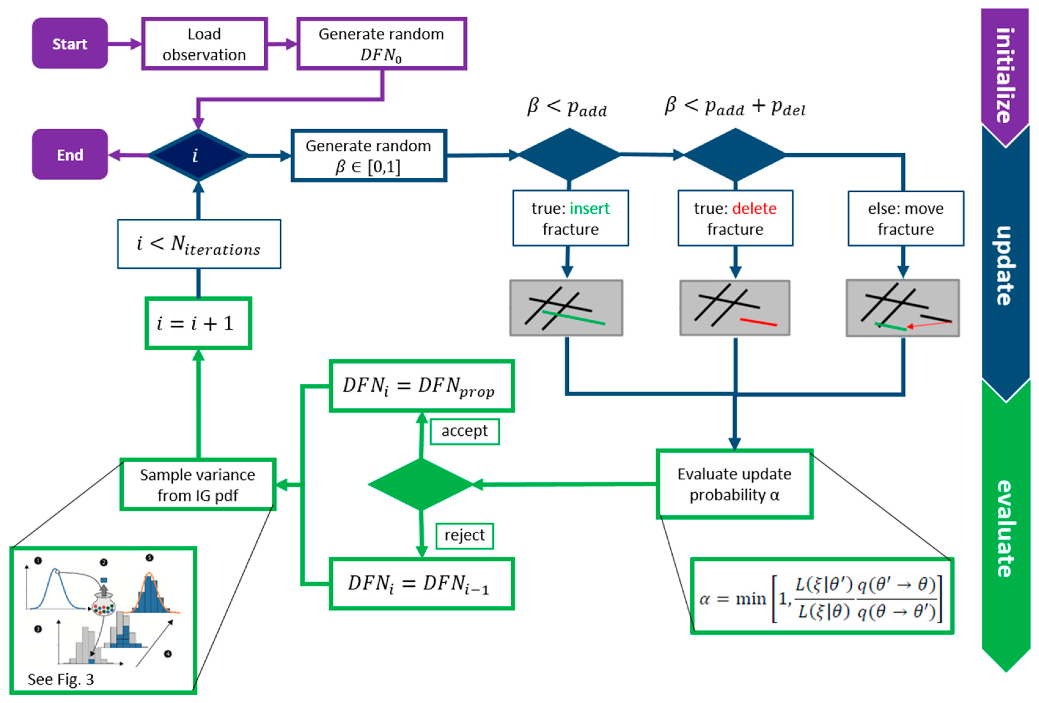
rjMCMC uses an iterative structure with two main phases per iteration; an update and an evaluation phase. The flowchart in Figure 2 describes the inversion procedure and the workflow of our inversion algorithm. In the update phase, the parameters of the DFN model are modified by one of the following updates: fracture movement, fracture insertion, and fracture deletion. The DFN model parameter set includes the number of fractures and for each fracture its position, the fracture inclination, and the fracture length. The parameter set of a DFN realization is denoted by θ . The dimension of the parameter space also changes, since the number of fractures varies through adding or deleting a fracture. This motivates the description of transdimensional inversion. We estimate the number of fractures during the iterations of the inversion to consider the computational costs of the inversion problem. The number of fractures is in the range of 10 to 10 2 and the dimension of the parameter space is three times the number of fractures. These parameters have to be adjusted by the inversion algorithm to reproduce the measured pressure signals or tracer breakthroughs.
The kind of update is randomly selected, with a predefined probability p a d d / p d e l / p s h i f t , which may change during the inversion process, e.g., if the fracture intensity is too high.
Fracture addition is the so-called birth move of the rjMCMC algorithm. For this update, first the DFN model gets discretized, adhering to a pre-defined spacing distance. This characteristic property of the fractured rock represents the shortest possible distance between two parallel fractures. A set of insertion points is identified based on this distance, where new fractures could be added. The insertion of fractures is only possible starting or intersecting with a given fracture since isolated fractures do not affect the transport. Counting the number of possible insertion points, we receive the insertion probability P i n s . The orientation, length, and physical properties of a new fracture are probabilistically chosen, based on the given characteristics of one or more fracture sets. In this study, a fracture set represents fractures with similar physical properties and inclinations (Table 1). The choice between different fracture sets is taken into account by the fracture set probability, P s e t . However, further constraints and properties may be defined, depending on the information that is available for a specific case. The fracture length is drawn from the fracture length distribution (FLD) that is assumed for the corresponding fracture set, which gives us the probability of the length of a new fracture, P l e n g t h .
The point of intersection along the fracture (fracture position) is randomly selected after the geometric properties of the fracture are determined. The new fracture is inserted in the field by assigning the fracture position to a random insertion point. We obtain the probability of the position P p o s where the new fracture intersects the existing DFN according to the number of possible points along the new fracture. The different probabilities, which have a part in the addition probability, are explained in detail in [40]. The resulting probability of fracture addition can be expressed as the product of the individual probabilities of the above-mentioned steps:
q a d d = P s e t P l e n g t h P i n s P p o s
Fracture deletion is the so-called death move of the rjMCMC algorithm. A randomly selected fracture gets deleted from the DFN model when it is applied. This update is constrained, only allowing the deletion of a fracture if the source and receiver points remain connected. This is required to properly run the forward model. The probability of this update reads as the reciprocal of the number of deletable fractures, n d e l e t a b l e   f r a c t u r e s :
q d e l = 1 n d e l e t a b l e   f r a c t u r e s
q a d d and q d e l are the transition probabilities. We receive the probability of the transition from the current DFN realization to a proposed realization by computing them. Therefore, q a d d and q d e l are the conditional probabilities of updating the DFN given the current realization.
Fracture movement is a straightforward update, representing a random perturbation of fracture coordinates. It does not change the dimension of the model parameter space. A fracture is randomly selected in our implementation, and is then shifted to another randomly drawn insertion point while using the same discretization as the fracture addition. Fracture movement updates symmetrically, that is, the probability of the forward and the reverse update is equal. The proposal ratio does not need to be calculated, because the fracture length and the fracture set will not change, i.e., only the likelihood ratio matters. In contrast, the parameters of a new fracture are drawn from the FLD and P s e t if we first delete a random fracture and add a new one in the next iteration. This requires the calculation of the proposal ratio for adding and deleting. Therefore, fracture moving necessitates less computational costs than adding or deleting. Hence, it is the most efficient update. This type of update is also known as the Metropolis update, as defined by Metropolis et al. [47].
The DFN model is iteratively adjusted in a loop that is based on the recorded pressure signals or tracer breakthroughs by one of the described updates, as it is shown in the flowchart (Figure 2). A proposed DFN model (denoted by the model parameters θ ) is evaluated while using the Metropolis-Hastings-Green acceptance criterion, i.e., the update probability α , comparing the current DFN realization (denoted by θ ) with the proposed DFN realization:
α = min [ 1 , P ( θ ) P ( θ ) L ( ξ | θ ) L ( ξ | θ ) q ( θ θ ) q ( θ θ ) | J | ] .
Equation (3) is calculated from the product of the prior ratio P ( θ ) / P ( θ ) , the likelihood ratio L ( ξ | θ ) / L ( ξ | θ ) the probability of the data given the model parameters, the proposal ratio q ( θ θ ) / q ( θ θ ) , and the determinant of the so-called Jacobian matrix | J | . The prior probability, multiplied by the likelihood function, yields the posterior probability, according to Bayes’ theorem. The Jacobian takes the change in the dimension of the parameter space into account, as provoked by fracture addition or fracture deletion. In the presented DFN inversion, the prior ratio is always equal to one, because, aside from the non-informative priors, all prior information is included in the proposal ratio. The likelihood ratio is calculated by dividing the likelihood function of the updated model by the non-updated model. The likelihood of a model can be expressed with the following Gaussian distribution if we assume that the observations are independent and follow a normal distribution:
L ( ξ | θ ) = 1 4 π σ 2 exp ( ( ξ f ( θ ) ) 2 2 σ 2 ) .
The transdimensional updates of the presented DFN inversion only deal with the discretized model parameter space. New fractures can only be inserted to discrete insertion points, with discretized fracture length distribution. Deleting a fracture from a DFN is also a discrete operation. The Jacobian matrix of these discrete updates is always equal to one [48]. This makes this inversion approach very efficient, as the transdimensional updates can be evaluated at the same computational cost as updates that do not change the dimension of the parameter space. For the same reason, the fracture spacing discretizes the originally continuous fracture length distribution, since discretized values ensure an easy computation of the Jacobian in the acceptance probability α , see Equation (3).
The MHG criteria ensure that the Markov chain is stationary, and it samples from the posterior probability distribution of the inverse problem. In our case, the MHG criteria simplify to:
α = min [ 1 , L ( ξ | θ ) L ( ξ | θ ) q ( θ θ ) q ( θ θ ) ] ,
which is the same as the acceptance ratio of the Metropolis–Hastings algorithm.
The accepted realization is stored and the Markov chain continues in step. In the case of rejection, the previous model gets restored and it is used for the start of the next iteration. The final result of the inversion is the ensemble of model realizations along the whole Markov chain. However, in practice, the first part of the chain (burn-in phase) is discarded, as these realizations are influenced by the chosen initial model until the chain converges [49].
The likelihood governs the convergence rate of the inversion. In this case, the control parameter of the inversion is a fixed variance σ 2 of the normal distribution in Equation (4). Choosing a smaller variance value could enhance the convergence rate, with the risk of trapping the algorithm early in the local minimum. We inspect the acceptance probability α to study the effect of the variance, σ 2 , on the convergence rate in more detail (Equation (3)). For this, we test the different settings of the variance. Note that, by changing the variance, only the likelihood ratio L r a t i o is affected, while the proposal and the prior ratio remain constant. First, we consider the case that the error between the observed and the current DFN simulated data decreases through a proposed realization. This yields a likelihood ratio that is greater than one, irrespective of whether a high or a low variance is chosen, and it induces a high acceptance probability.
Second, we suppose the choice of a high variance. The limit of R M S c u r r e n t 2 R M S p r o p o s e d 2 2 σ 2 , is zero, as σ 2 approaches infinite,
lim σ 2 R M S c u r r e n t 2 R M S p r o p o s e d 2 2 σ 2 = 0 ,
and therefore, the limit of L r a t i o is one ( lim σ 2 L r a t i o = 1 ) . Hence, the use of a high variance causes a high acceptance rate
a c c = N a c c e p t e d N i t e r a t i o n s
independent of whether RMS becomes smaller or larger through the proposed DFN.
In contrast, the lower the variance is, the lower the mean RMS after the burn-in phase. However, a variance that is too low increases the possibility of the algorithm getting stuck in a local minimum as L r a t i o approaches infinity for a decreasing error and zero for an increasing RMS while using small variance. If a higher variance is chosen, the mean RMS increases as well, but more proposed realizations will be accepted and the mixing of different accepted realizations is better.

2.3. Estimation of the Noise Variance

In addition to the reconstruction of the DFN, we can estimate the variance of the measurement error, i.e., the measurement noise. While this value is the main control parameter of the convergence of the rjMCMC algorithm, in most implementations its value is empirically chosen. For pressure measurements, this value is relatively easy to properly choose, but for solute and especially for temperature measurements, it becomes difficult due to numerous environmental factors and the strong influence of imperfect experimental conditions (e.g., nonuniform physical properties of the borehole, sampling inconsistency, tracer degradation). Hence, we apply the following methodology for variance sampling: The measured data ξ o b s (obtained by n measurement points) is composed of the breakthrough curves (BTC) or the pressure signals that would be observed without noise ξ ˜ and a measurement error ε . Therefore, the recorded data can be expressed as ξ o b s = ξ ˜ + ε . ε i ( i = 1 , , n ) is independent and normally distributed, ε i N ( 0 ,   σ n o i s e 2 ) . The observation data is also normally distributed ξ o b s , i N ( ξ ˜ i , σ n o i s e 2 ) with data mean ξ ˜ and noise variance σ n o i s e 2 .
Our aim is to determine ξ ˜ and estimate the variance of the noise. Therefore, we need a probability density function (pdf) for σ n o i s e 2 that depends on the observed data and the model parameters to draw the variance from. The posterior pdf of σ n o i s e 2 can be calculated while using Bayes’ theorem with the model parameters θ (DFN and inversion parameters) and the observation data ξ o b s
p ( θ | ξ o b s ) = p ( ξ o b s | θ ) p ( θ ) p ( ξ o b s ) .
The denominator is assumed as constant and therefore can be neglected. For reasons of clarity, θ σ n o i s e 2 denotes the model parameters without σ n o i s e 2 . Due to Bayes’ theorem and a constant p ( ξ o b s ) , the posterior pdf of σ n o i s e 2 can be expressed as
p ( σ n o i s e 2 | ξ o b s ,   θ σ n o i s e 2 )     p ( ξ o b s | σ n o i s e 2 ,   θ σ n o i s e 2 )   p ( σ n o i s e 2 )
from which σ n o i s e 2 can be sampled [50,51].
To determine the likelihood function p ( ξ o b s | σ n o i s e 2 ,   θ σ n o i s e 2 ) , we assume that the breakthrough curves or the pressure signals of the current DFN realization (denoted by f ( θ ) ) calculated with the forward model are the data mean ξ ˜ . This assumption is valid after the burn-in phase, because the error between the data mean and the simulated data from the proposed DFN realization is small enough ξ ˜ i f ( θ ) i 0 . Therefore, the probability density function of the observation data given the model parameters, i.e., the likelihood function, can be calculated with Equation (4). The estimated variance is higher than the variance of the noise at the beginning of the inversion due to the higher error occurring during the first iterations, i.e., the burn-in phase. The estimated noise variance is inserted into the likelihood function to replace the fixed variance. This is valid because of the assumption ξ o b s , i     N ( ξ ˜ i , σ n o i s e 2 ) , which is expressed by the likelihood function. Thus, the variance in the likelihood function is updated by estimating the noise variance in every iteration of the rjMCMC loop.
The use of a noninformative prior as pdf of σ n o i s e 2 ensures that the data mainly affect the posterior distribution. In this study, an inverse gamma (IG) and a uniform (U) prior are applied
p ( σ n o i s e 2 ) I G ( a , b ) ,
p ( σ n o i s e 2 ) U ( 0 , c ) ,
with the so-called hyperparameters a , b , and c ( a , b , c > 0 ). A noninformative prior is obtained by using small values for a and high values for b and c . Bayes’ theorem leads to the following posterior pdfs that are dependent on the prior
p ( σ n o i s e 2 | ξ o b s , θ σ n o i s e 2 ) I G ( a + n 2 , b + i = 1 n ( ξ o b s , i f ( θ ) i ) 2 2 ) ,
p ( σ n o i s e 2 | ξ o b s , θ σ n o i s e 2 ) I G ( n 2 1 ,   i = 1 n ( ξ o b s , i f ( θ ) i ) 2 2 ) .
The calculation of the posterior pdf is illustrated in Equation (12) while using the IG prior and in Equation (13) using the uniform prior. The IG prior has to be carefully handled, since the pdf is improper as a and 1 / b approach zero. A pdf is improper if the integral of the distribution is infinity, which violates the assumption that the cumulative probability distribution approaches one or any positive value for non-normalized distributions. In this case, the improper IG prior leads to improper posterior distribution. The results of the two different priors will be compared in the following because of this potential shortcoming [50,51].
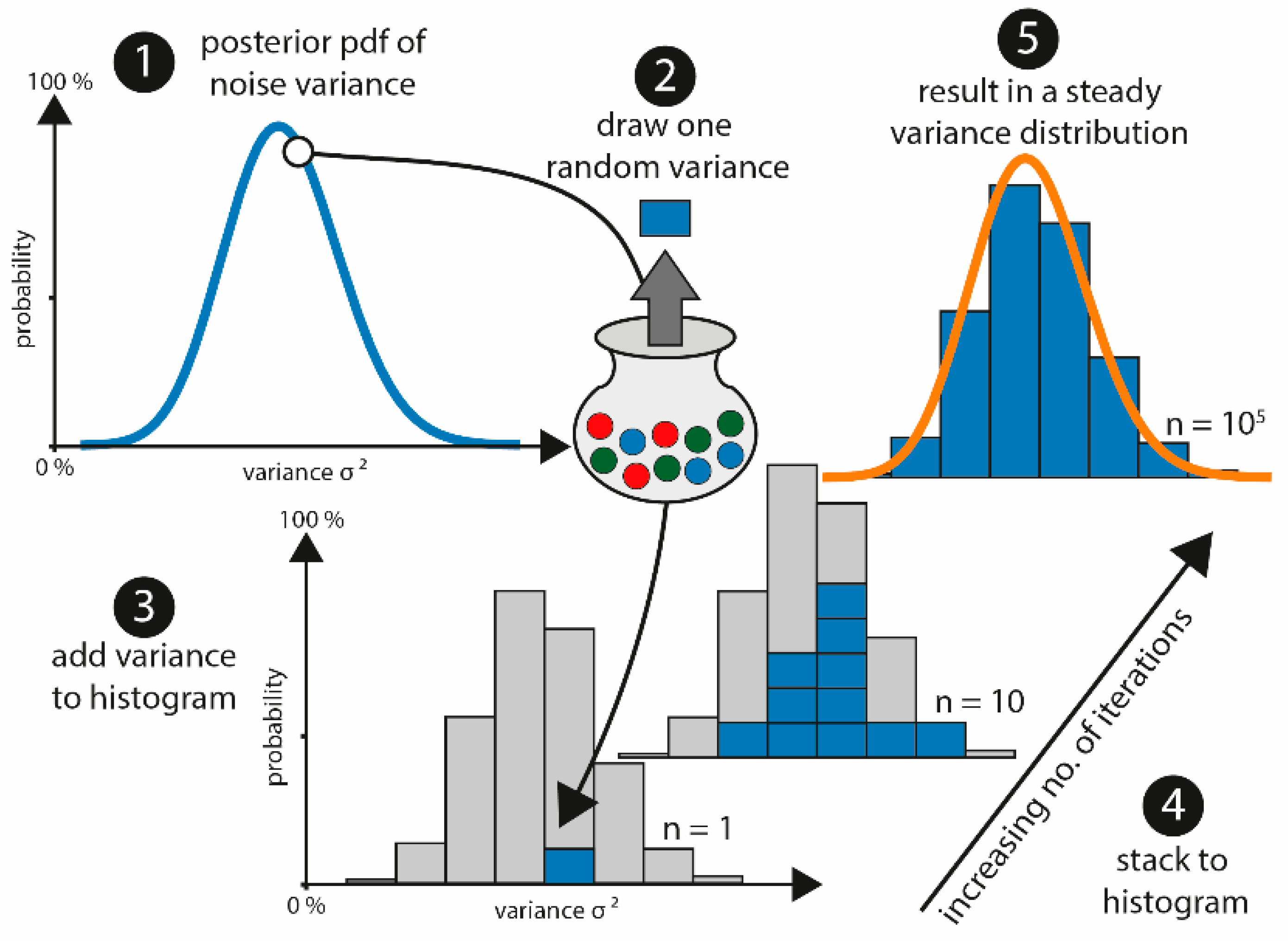
After a new DFN realization is accepted or rejected (as explained in Section 2.2), the variance is estimated from the posterior pdf while using the Gibbs sampling method illustrated in Figure 3. The acceptance probability α of a Gibbs sampler is always one. Therefore, every proposed variance will be accepted [49]. The variance sampling is implemented in every iteration of the inversion loop after the evaluation of a proposed update of the DFN model parameters (see Figure 2). This is illustrated by adding the sampled variances to a histogram, as shown in step 4 of Figure 3. The described procedure is presented for an increasing number of iterations.
A similar procedure is employed by Fearnhead [52] and Punskaya et al. [53] to analyze a speech signal in order to obtain the real speech data without noise. Gallagher et al. [54] used the rjMCMC method to identify the abrupt changes in geochemical data series due to environmental or climatic variations and to fit a constant regression function to the recorded data curves. The regression function is defined piecewise between two changepoints, which model the abrupt changes in the data series. Adding, deleting, or moving a changepoint estimates the number and position of the changepoints. They estimate the variance of the noise while using an acceptance criterion to accept or reject a new variance proposal. In Sambridge [55], an rjMCMC algorithm is applied to reconstruct sea level variations assuming that the time series and the measured data contain stochastic noise.

3. Results

In the following, we first rely on a fixed variance in the likelihood function to compare the results of hydraulic and tracer tomography. In the second part, the results of the estimation of the noise variance are presented.

3.1. Results of the DFN Inversion

The result of the DFN inversion is not a single calibrated DFN model. In every iteration of the MCMC loop, a DFN realization is calculated and stored. The set of DFN realizations is called the ensemble. This result contains information regarding the probabilistic properties of the inverse problem, such as uncertainty and bi- or multimodality. The probabilistic characteristics stay the same for different inversion runs, as our inversion method is a stochastic method. To visualize the ensemble, we convert it to a fracture probability map [40]. This is done via the rasterization of the DFN realizations and by taking the mean of these raster models over the ensemble. The fracture probability of one point, i.e., the probability of this position to contain a fracture, is the number of DFN realizations that identify a fracture at this point divided by the whole number of realizations. This representation is equivalent to taking the mean of the ensemble, which is a common method of visualization (see [12,56]).
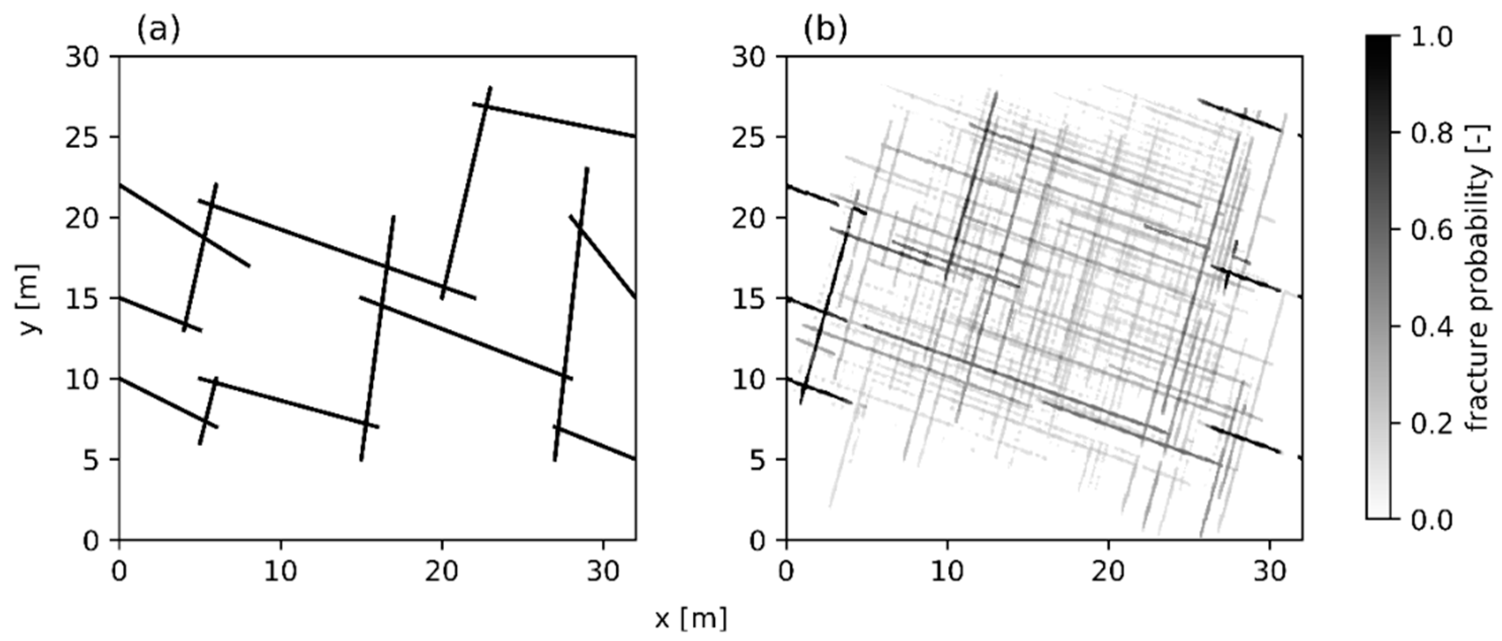
Figure 4 shows the tomographic reconstruction of the hydraulic tomography experiment. The fracture locations are well resolved, and the locations of the fracture intersections with the higher fracture probability roughly match those of the synthetic model. Fractures at the sides of the model (connecting the sources and receivers with the DFN) are fixed, thus they appear with 100% probability. This assumption is acceptable since it is possible to detect the fracture location and orientation in boreholes based on core and image logs (e.g., optical or acoustical televiewer) (see [45,57]).
The fracture probability map only shows the fractures with a probability higher than 10 % to present the results clearly. In Figure 4, the general characteristics of the original DFN can be identified. We can locate the area where the main horizontal connection between the source and receiver takes place. In addition, the non-fractured positions can be detected. Still, some errors are visible in the reconstruction. The quality of the recognition is better there so that the fractures on the right half of the model appear with higher probability because observation points are only placed on the right side of the model. The position of the fractures, which connect the fractures of the left side of the model horizontally with the middle of the investigated area, is uniformly distributed between y 8 m and y 22 m . Therefore, we can conclude that this area contains fractures, but we cannot determine the exact position of a single fracture. In contrast, the position of the fractures, which horizontally connect the middle of the area with the right side of the model, has a higher probability and it is better resolved. The variance of a fracture position is much smaller on the right half of the investigated area. The position of the fracture with its center point at x 30 m and y 12 m can be fit to a normal distribution, since the fractures at the left and right side of it appear symmetrically with a decreasing probability. This corresponds to a Gaussian pdf of the position of this fracture. The aligned dots occur due to the rasterization in the fracture probability, and their size depends on the accuracy of converting a continuous DFN realization to the grid points of the probability raster. They represent fractures with a very low probability.
Figure 5 shows the tomographic reconstruction of the tracer tomography experiment. We check the acceptance rate of the rjMCMC loop after the burn-in phase to ensure that both of the results are comparable, see Equation (7). The acceptance rate in both cases is about a c c 4.2 % . From this, we can conclude that the different results of the different tomographic concepts do not depend on the parameter settings of the inversion, and especially not on the variance in the likelihood function. The most obvious difference to the hydraulic tomography example is the larger variability of the results. In contrast to the results of the hydraulic tomography (Figure 4), single fractures, except for fractures from the injection and receiver points, are less visible, since no fractures occur with a high probability. Additionally, neither the left nor the right side is resolved well with a high probability. Still, from the result in Figure 5, we get an idea regarding the fractured and non-fractured areas and the main characteristics of the DFN. The gaps appearing between some of the pixels are a matter of rasterization similar to the aligned dots and they do not occur in the individual DFN realizations. This results from a raster grid that does not accord well with the DFN geometry.

3.2. Results Estimating the Noise Variance

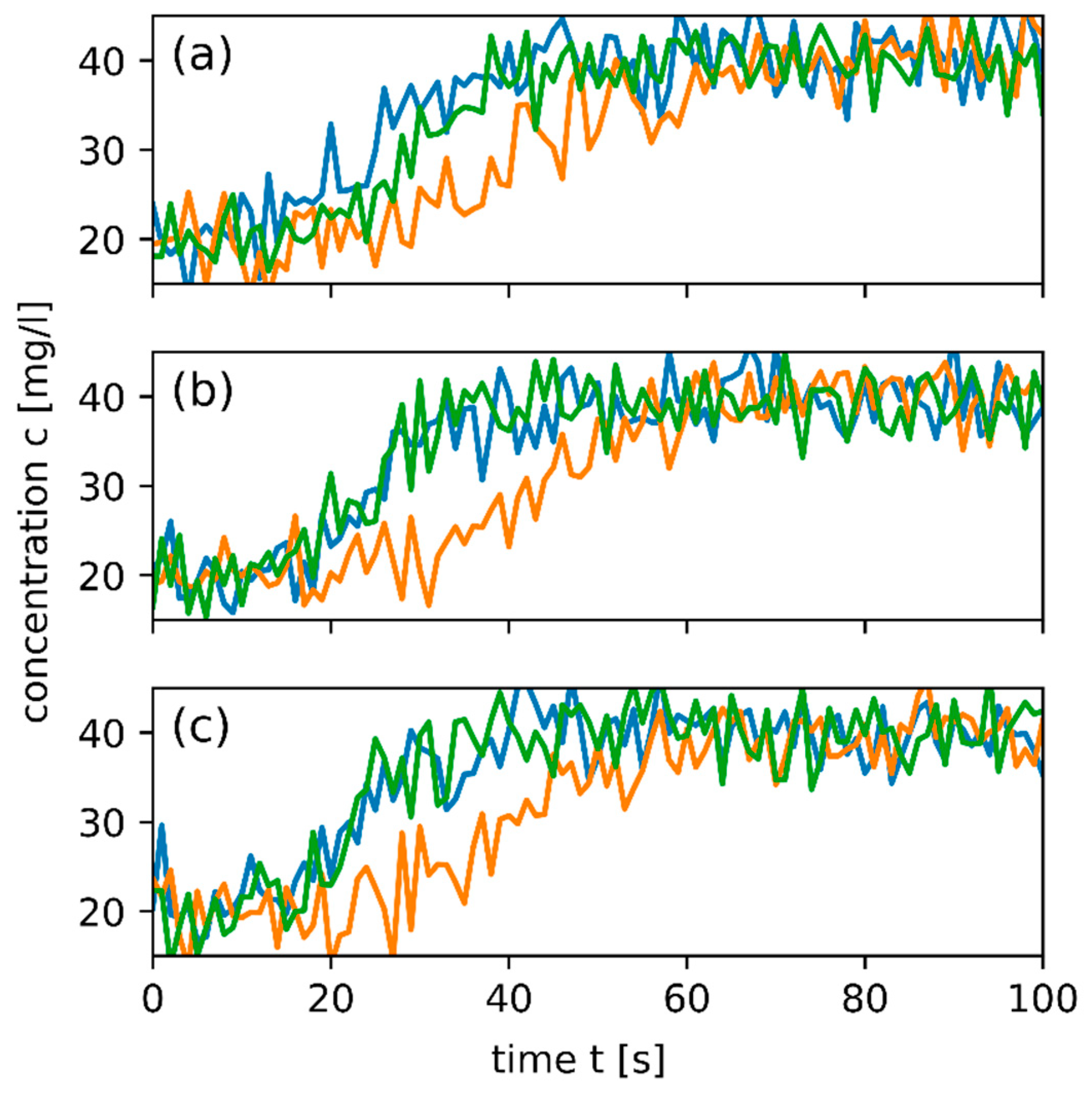
In contrast to the previous section, we assume that the observed tracer breakthroughs and pressure signals contain stochastic noise. Therefore, we want not only to do the inversion of the DFN, but to also estimate the noise variance and the data mean, i.e., the theoretically measured data without noise. This is accomplished according to Section 2.3. A synthetic example for noisy tracer breakthroughs with σ n o i s e = 3 is shown in Figure 6.
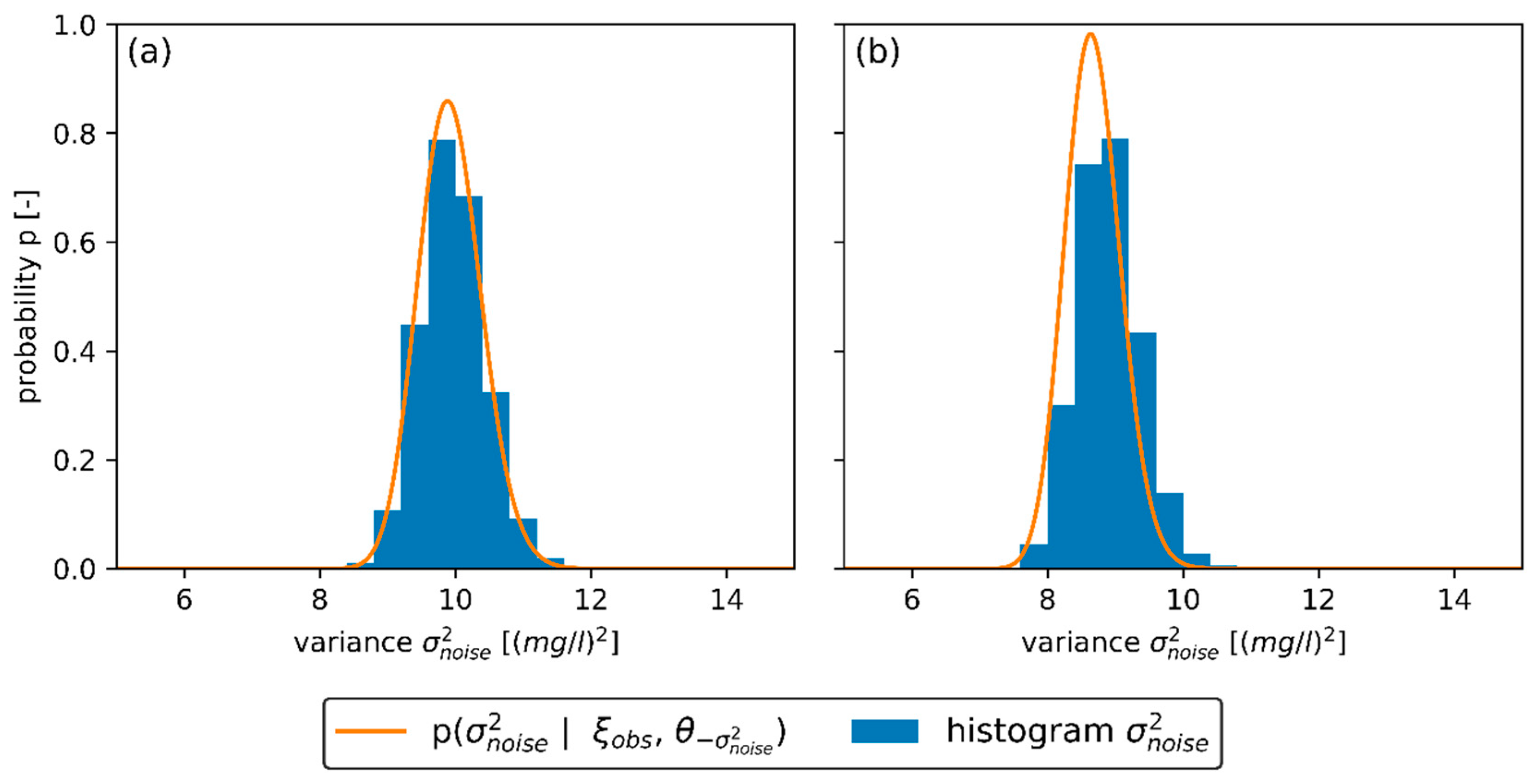
The data mean is iteratively estimated by the inversion of the DFN by applying the forward model to calculate the tracer breakthroughs of the current DFN realization. The variance is sampled from the IG posterior pdf in every iteration of the inversion loop. These samples are illustrated in a histogram that compares this with the posterior pdf of σ n o i s e 2 p ( σ n o i s e 2 | ξ o b s ,   θ σ n o i s e 2 ) of the last iteration of the rjMCMC loop in Figure 7. The pdf and the histogram in Figure 6 are as well not normalized, i.e., a cumulative probability function would approach any positive value for an increasing variance due to the non-normalized posterior pdf (see Equation (9)) from which the variance is sampled. The samples converge to a stationary distribution, since the histogram of the variance samples fulfills the posterior pdf of the last step. Both variance histograms are similar, as we compare the two different priors. Hence, we can conclude that both priors are in fact noninformative, because the posterior pdf is mainly affected by the data and not by the choice of the prior pdf. In addition, the prior IG pdf does not lead to an improper subsequent pdf in this case.
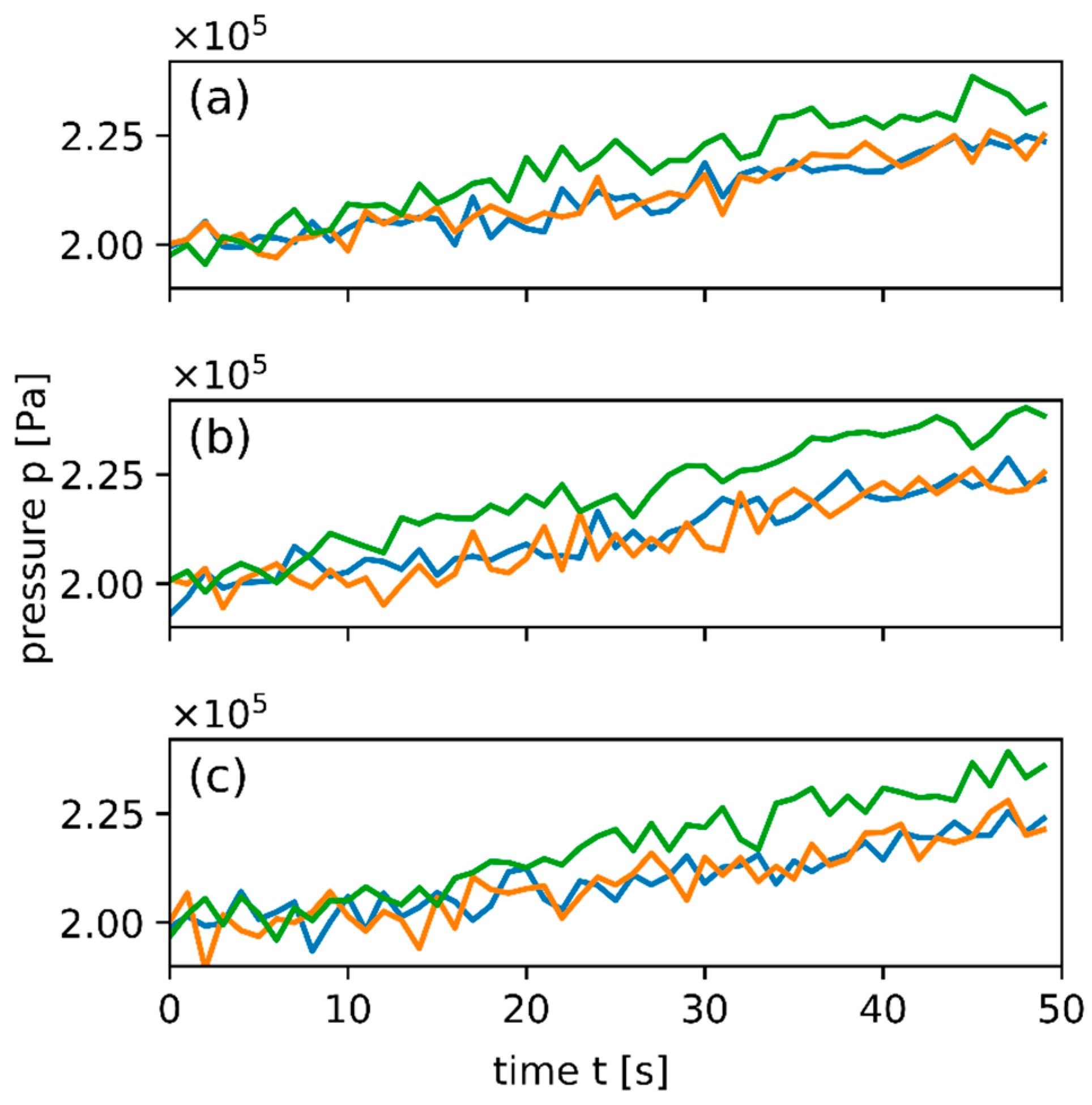
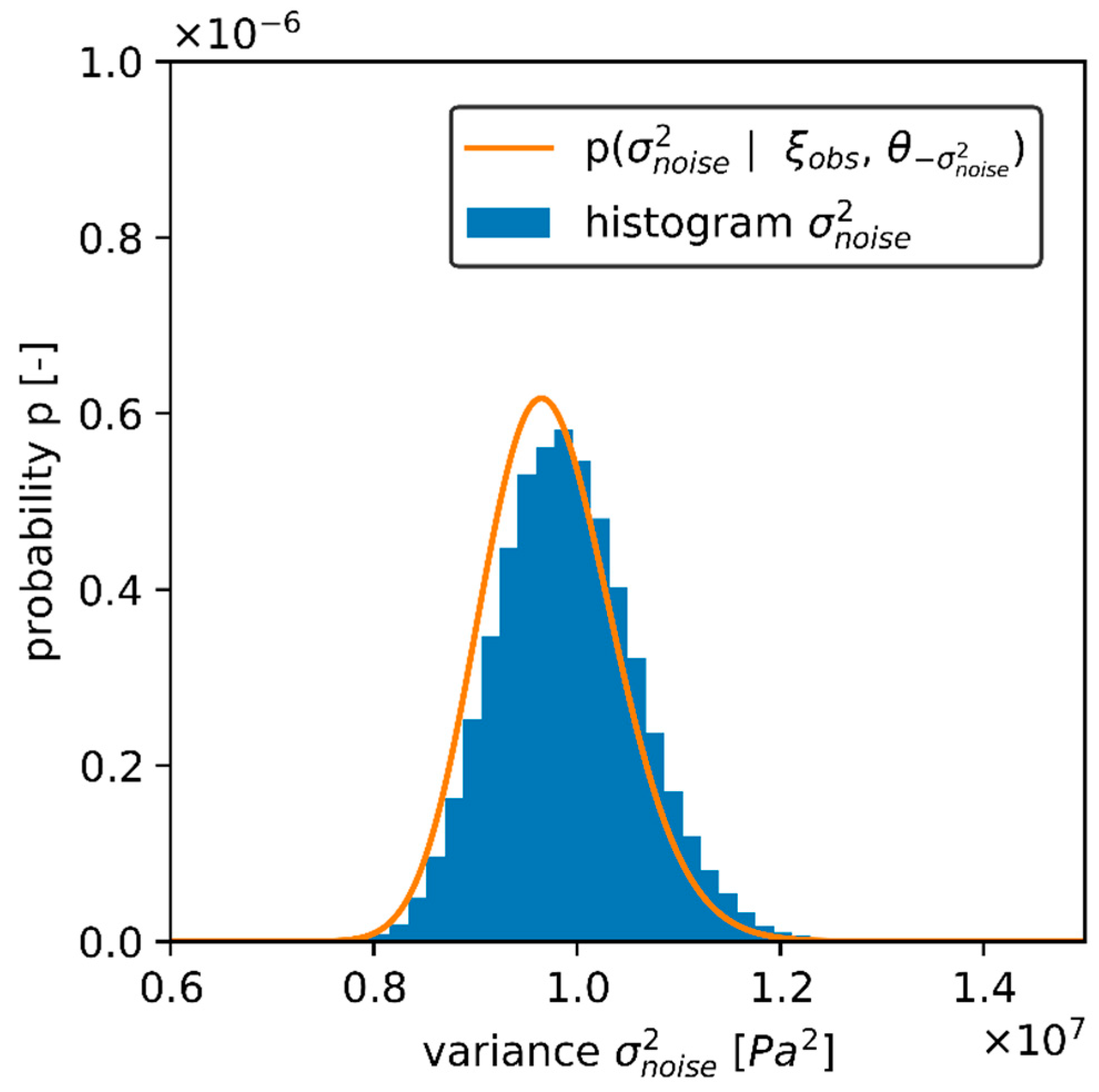
The same procedure could be applied to the noisy pressure signals (Figure 8). The histogram of the variance samples and the posterior pdf of σ n o i s e 2 are shown in Figure 9. Additionally, in this case, both of the priors provide similar histograms and posterior pdfs of σ n o i s e 2 .

4. Discussion and Conclusions

The presented study deals with an exemplary hypothetical case, which makes it difficult to generalize the results to other experimental setups or general conclusions. Still, the application of the two tomographic concepts allows for the comparison of characteristic differences. Hydraulic tomography provides better results than tracer tomography, since the variability of the result is smaller and some fractures occur with a higher probability, i.e., the obtained fracture probability map of the hydraulic tomography is better resolved. In this case, the pressure signals are better for the inversion, because the complexity of the simulation is smaller. For practical use, many extra factors would probably make the tracer tomography better, e.g., the measurement noise is smaller, and tracer breakthrough curves can be more easily detected. Both tomographic concepts are able to perfectly identify no fractured areas and the main characteristics. The experiment should be repeated in the other direction, since the part of the cross-sectional area where the receiver points are located provides better results to further improve our inversion algorithm. This uneven sensitivity is a known attribute of tomographic methods, as it was shown for continuous reconstruction in [20].
The presented procedure for the estimation of variance includes noise variance and model errors. The estimated variance is usually higher than the variance of the noise, since the estimated variance includes not only the variance of the noise, but also the error of the conceptual model, e.g., the geometrical constraints (only two different fracture inclinations, fracture length distribution), the limited number of iterations, and errors of the forward model. Therefore, this method could also be applied to determine the errors of the conceptual model, if observation data without noise or with very low noise variances are used for the inversion.
Variance estimation becomes even more significant when considering, for instance, heat as a tracer. In-situ temperature observations are more prone to systematic errors and to being affected by diffusion than solutes. The simulation of thermal transport in both fracture and matrix introduces an extra level of complexity into the forward model, and requires the specification of additional physical parameters. Variance estimation could be employed to reveal initial improper settings if these parameters are set incorrectly.
The aim of this study is to extend the inversion procedure from synthetic DFN cases to practical applications with field data. To prepare this, we conclude from the synthetic DFN case study to the parameters and information we need to use this inversion algorithm in practice. In addition, we checked the limitations and the conceptual errors of this approach. However, we introduce a method to deal with that issue. One conclusion is that we need a 3D forward model to expand from the two-dimensional cases to three-dimensional DFN reconstruction. Moreover, we require information regarding the fracture sets, e.g., from outcrops. We also have to use an optical or acoustical televiewer to get the inclination and the position of the fractures adjacent to the boreholes to introduce them as source and receivers for the inversion and as boundary conditions in the forward model.

Author Contributions

Formal analysis, L.M.R., M.S., M.J. and P.B.; Investigation, L.M.R., M.S., M.J. and P.B.; Methodology, L.M.R., M.S., M.J. and P.B.; Writing–original draft, L.M.R., M.S. and P.B.; Writing–review & editing, M.J. and P.B. All authors contributed equally to the paper.

Funding

This research was funded by the German Research Foundation (DFG), grant number BA-2850-5-1.

Acknowledgments

We thank Jakob Michael for language editing and Hannes Hemmerle for his help designing Figure 3. We also would like to thank the two anonymous reviewers for their constructive and useful comments.

Conflicts of Interest

The authors declare no conflict of interest.

References

  1. Berg, S.J.; Illman, W.A. Three-dimensional transient hydraulic tomography in a highly heterogeneous glaciofluvial aquifer-aquitard system. Water Resour. Res. 2011, 47. [Google Scholar] [CrossRef]
  2. Brauchler, R.; Hu, R.; Hu, L.; Jiménez, S.; Bayer, P.; Dietrich, P.; Ptak, T. Rapid field application of hydraulic tomography for resolving aquifer heterogeneity in unconsolidated sediments. Water Resour. Res. 2013, 49. [Google Scholar] [CrossRef]
  3. Cardiff, M.; Barrash, W.; Kitanidis, P.K. A field proof-of-concept of aquifer imaging using 3-D transient hydraulic tomography with modular, temporarily-emplaced equipment. Water Resour. Res. 2012, 48. [Google Scholar] [CrossRef] [Green Version]
  4. Jiménez, S.; Brauchler, R.; Bayer, P. A new sequential procedure for hydraulic tomographic inversion. Adv. Water Resour. 2013, 62, 59–70. [Google Scholar] [CrossRef]
  5. Illman, W.A. Hydraulic tomography offers improved imaging of heterogeneity in fractured rocks. Groundwater 2014, 52, 659–684. [Google Scholar] [CrossRef]
  6. Zha, Y.; Yeh, T.C.J.; Illman, W.A.; Zeng, W.; Zhang, Y.; Sun, F.; Shi, L. A Reduced-Order Successive Linear Estimator for Geostatistical Inversion and its Application in Hydraulic Tomography. Water Resour. Res. 2018, 54, 1616–1632. [Google Scholar] [CrossRef]
  7. Hu, L.; Bayer, P.; Alt-Epping, P.; Tatomir, A.; Sauter, M.; Brauchler, R. Time-lapse pressure tomography for characterizing CO2 plume evolution in a deep saline aquifer. Int. J. Greenh. Gas Control 2015, 39, 91–106. [Google Scholar] [CrossRef]
  8. Hu, L.; Bayer, P.; Brauchler, R. Detection of carbon dioxide leakage during injection in deep saline formations by pressure tomography. Water Resour. Res. 2016, 52, 5676–5686. [Google Scholar] [CrossRef]
  9. Vesselinov, V.V.; Neuman, S.P.; Illman, W.A. Three-dimensional numerical inversion of pneumatic cross-hole tests in unsaturated fractured tuff: 1. Methodology and borehole effects. Water Resour. Res. 2001, 37, 3001–3017. [Google Scholar] [CrossRef]
  10. Ni, C.-F.; Yeh, T.-C.J. Stochastic inversion of pneumatic cross-hole tests and barometric pressure fluctuations in heterogeneous unsaturated formations. Adv. Water Resour. 2008, 31, 1708–1718. [Google Scholar] [CrossRef]
  11. Datta-Gupta, A.; Yoon, S.; Vasco, D.W.; Pope, G.A. Inverse modeling of partitioning interwell tracer tests: A streamline approach. Water Resour. Res. 2002, 38. [Google Scholar] [CrossRef]
  12. Jiménez, S.; Mariethoz, G.; Brauchler, R.; Bayer, P. Smart pilot points using reversible-jump Markov-chain Monte Carlo. Water Resour. Res. 2016, 52, 3966–3983. [Google Scholar] [CrossRef] [Green Version]
  13. Ma, R.; Zheng, C.; Zachara, J.M.; Tonkin, M. Utility of bromide and heat tracers for aquifer characterization affected by highly transient flow conditions. Water Resour. Res. 2012, 48. [Google Scholar] [CrossRef]
  14. Doetsch, J.; Linde, N.; Vogt, T.; Binley, A.; Green, A.G. Imaging and quantifying salt-tracer transport in a riparian groundwater system by means of 3D ERT monitoring. Geophysics 2012, 77, B207–B218. [Google Scholar] [CrossRef] [Green Version]
  15. Jardani, A.; Revil, A.; Dupont, J. Stochastic joint inversion of hydrogeophysical data for salt tracer test monitoring and hydraulic conductivity imaging. Adv. Water Resour. 2013, 52, 62–77. [Google Scholar] [CrossRef]
  16. Jougnot, D.; Jiménez-Martínez, J.; Legendre, R.; Le Borgne, T.; Méheust, Y.; Linde, N. Impact of small-scale saline tracer heterogeneity on electrical resistivity monitoring in fully and partially saturated porous media: Insights from geoelectrical milli-fluidic experiments. Adv. Water Resour. 2018, 113, 295–309. [Google Scholar] [CrossRef] [Green Version]
  17. Singha, K.; Gorelick, S.M. Saline tracer visualized with three-dimensional electrical resistivity tomography: Field-scale spatial moment analysis. Water Resour. Res. 2005, 41. [Google Scholar] [CrossRef]
  18. Hermans, T.; Wildemeersch, S.; Jamin, P.; Orban, P.; Brouyère, S.; Dassargues, A.; Nguyen, F. Quantitative temperature monitoring of a heat tracing experiment using cross-borehole ERT. Geothermics 2015, 53, 14–26. [Google Scholar] [CrossRef] [Green Version]
  19. Schwede, R.L.; Li, W.; Leven, C.; Cirpka, O.A. Three-dimensional geostatistical inversion of synthetic tomographic pumping and heat-tracer tests in a nested-cell setup. Adv. Water Resour. 2014, 63, 77–90. [Google Scholar] [CrossRef]
  20. Somogyvári, M.; Bayer, P.; Brauchler, R. Travel-time-based thermal tracer tomography. Hydrol. Earth Syst. Sci. 2016, 20, 1885–1901. [Google Scholar] [CrossRef] [Green Version]
  21. Klepikova, M.V.; Le Borgne, T.; Bour, O.; Gallagher, K.; Hochreutener, R.; Lavenant, N. Passive temperature tomography experiments to characterize transmissivity and connectivity of preferential flow paths in fractured media. J. Hydrol. 2014, 512, 549–562. [Google Scholar] [CrossRef] [Green Version]
  22. Cardiff, M.; Barrash, W.; Kitanidis, P.K. Hydraulic conductivity imaging from 3-D transient hydraulic tomography at several pumping/observation densities. Water Resour. Res. 2013, 49, 7311–7326. [Google Scholar] [CrossRef] [Green Version]
  23. Bohling, G.C.; Butler, J.J.; Zhan, X.; Knoll, M.D. A field assessment of the value of steady shape hydraulic tomography for characterization of aquifer heterogeneities. Water Resour. Res. 2007, 43. [Google Scholar] [CrossRef] [Green Version]
  24. Paradis, D.; Gloaguen, E.; Lefebvre, R.; Giroux, B. A field proof-of-concept of tomographic slug tests in an anisotropic littoral aquifer. J. Hydrol. 2016, 536, 61–73. [Google Scholar] [CrossRef]
  25. Somogyvári, M.; Bayer, P. Field validation of thermal tracer tomography for reconstruction of aquifer heterogeneity. Water Resour. Res. 2017, 53, 5070–5084. [Google Scholar] [CrossRef]
  26. Tso, C.H.M.; Zha, Y.; Yeh, T.C.J.; Wen, J.C. The relative importance of head, flux, and prior information in hydraulic tomography analysis. Water Resour. Res. 2016, 52, 3–20. [Google Scholar]
  27. Zhao, Z.; Illman, W.A.; Yeh, T.C.J.; Berg, S.J.; Mao, D. Validation of hydraulic tomography in an unconfined aquifer: A controlled sandbox study. Water Resour. Res. 2015, 51, 4137–4155. [Google Scholar] [CrossRef]
  28. Hu, R.; Brauchler, R.; Herold, M.; Bayer, P. Hydraulic tomography analog outcrop study: Combining travel time and steady shape inversion. J. Hydrol. 2011, 409, 350–362. [Google Scholar] [CrossRef]
  29. Hao, Y.; Yeh, T.C.J.; Xiang, J.; Illman, W.A.; Ando, K.; Hsu, K.C.; Lee, C.H. Hydraulic tomography for detecting fracture zone connectivity. Groundwater 2008, 46, 183–192. [Google Scholar] [CrossRef]
  30. Illman, W.A. Lessons learned from hydraulic and pneumatic tomography in fractured rocks. Procedia Environ. Sci. 2015, 25, 127–134. [Google Scholar] [CrossRef]
  31. Illman, W.A.; Liu, X.; Takeuchi, S.; Yeh, T.C.J.; Ando, K.; Saegusa, H. Hydraulic tomography in fractured granite: Mizunami Underground Research site, Japan. Water Resour. Res. 2009, 45. [Google Scholar] [CrossRef] [Green Version]
  32. Zha, Y.; Yeh, T.-C.J.; Illman, W.A.; Tanaka, T.; Bruines, P.; Onoe, H.; Saegusa, H. What does hydraulic tomography tell us about fractured geological media? A field study and synthetic experiments. J. Hydrol. 2015, 531, 17–30. [Google Scholar] [CrossRef]
  33. Dong, Y.; Fu, Y.; Yeh, T.C.J.; Wang, Y.L.; Zha, Y.; Wang, L.; Hao, Y. Equivalence of Discrete Fracture Network and Porous Media Models by Hydraulic Tomography. Water Resour. Res. 2019. [Google Scholar] [CrossRef]
  34. Wen, J.C.; Chen, J.L.; Yeh, T.C.J.; Wang, Y.L.; Huang, S.Y.; Tian, Z.; Yu, C.Y. Redundant and non-redundant information for Model Calibration or Hydraulic Tomography. Groundwater 2019. [Google Scholar] [CrossRef] [PubMed]
  35. Wang, X.; Jardani, A.; Jourde, H. A hybrid inverse method for hydraulic tomography in fractured and karstic media. J. Hydrol. 2017, 551, 29–46. [Google Scholar] [CrossRef]
  36. Brauchler, R.; Böhm, G.; Leven, C.; Dietrich, P.; Sauter, M. A laboratory study of tracer tomography. Hydrogeol. J. 2013, 21, 1265–1274. [Google Scholar] [CrossRef]
  37. Fischer, P.; Jardani, A.; Wang, X.; Jourde, H.; Lecoq, N. Identifying Flow Networks in a Karstified Aquifer by Application of the Cellular Automata-Based Deterministic Inversion Method (Lez Aquifer, France). Water Resour. Res. 2017, 53, 10508–10522. [Google Scholar] [CrossRef]
  38. Fischer, P.; Jardani, A.; Jourde, H.; Cardiff, M.; Wang, X.; Chedeville, S.; Lecoq, N. Harmonic pumping tomography applied to image the hydraulic properties and interpret the connectivity of a karstic and fractured aquifer (Lez aquifer, France). Adv. Water Resour. 2018, 119, 227–244. [Google Scholar] [CrossRef]
  39. Fischer, P.; Jardani, A.; Lecoq, N. Hydraulic tomography of discrete networks of conduits and fractures in a karstic aquifer by using a deterministic inversion algorithm. Adv. Water Resour. 2018, 112, 83–94. [Google Scholar] [CrossRef]
  40. Somogyvári, M.; Jalali, M.; Jimenez Parras, S.; Bayer, P. Synthetic fracture network characterization with transdimensional inversion. Water Resour. Res. 2017, 53, 5104–5123. [Google Scholar] [CrossRef]
  41. Dorn, C.; Linde, N.; Le Borgne, T.; Bour, O.; Baron, L. Single-hole GPR reflection imaging of solute transport in a granitic aquifer. Geophys. Res. Lett. 2011, 38. [Google Scholar] [CrossRef] [Green Version]
  42. Chuang, P.-Y.; Chia, Y.; Chiu, Y.-C.; Teng, M.-H.; Liou, S.Y.H. Mapping fracture flow paths with a nanoscale zero-valent iron tracer test and a flowmeter test. Hydrogeol. J. 2018, 26, 321–331. [Google Scholar] [CrossRef]
  43. Ziegler, M.; Loew, S.; Moore, J.R. Distribution and inferred age of exfoliation joints in the Aar Granite of the central Swiss Alps and relationship to Quaternary landscape evolution. Geomorphology 2013, 201, 344–362. [Google Scholar] [CrossRef]
  44. Jalali, M. Thermo-Hydro-Mechanical Behavior of Conductive Fractures Using a Hybrid Finite Difference—Displacement Discontinuity Method; University of Waterloo Library: Waterloo, ON, Canada, 2013. [Google Scholar]
  45. Afshari Moein, M.J.; Somogyvári, M.; Valley, B.; Jalali, M.; Loew, S.; Bayer, P. Fracture Network Characterization Using Stress-Based Tomography. J. Geophys. Res. Solid Earth 2018, 123, 9324–9340. [Google Scholar] [CrossRef]
  46. Green, P.J. Reversible jump Markov chain Monte Carlo computation and Bayesian model determination. Biometrika 1995, 82, 711–732. [Google Scholar] [CrossRef]
  47. Metropolis, N.; Rosenbluth, A.W.; Rosenbluth, M.N.; Teller, A.H.; Teller, E. Equation of state calculations by fast computing machines. J. Chem. Phys. 1953, 21, 1087–1092. [Google Scholar] [CrossRef]
  48. Denison, D.G.; Holmes, C.C.; Mallick, B.K.; Smith, A.F. Bayesian Methods for Nonlinear Classification and Regression; John Wiley & Sons: Hoboken, NJ, USA, 2002; Volume 386. [Google Scholar]
  49. Brooks, S.; Gelman, A.; Jones, G.; Meng, X.-L. Handbook of Markov Chain Monte Carlo; CRC Press: Boca Raton, FL, USA, 2011. [Google Scholar]
  50. Gelman, A.; Stern, H.S.; Carlin, J.B.; Dunson, D.B.; Vehtari, A.; Rubin, D.B. Bayesian Data Analysis; Chapman and Hall/CRC: Boca Raton, FL, USA, 2013. [Google Scholar]
  51. Demirhan, H.; Kalaylioglu, Z. Joint prior distributions for variance parameters in Bayesian analysis of normal hierarchical models. J. Multivar. Anal. 2015, 135, 163–174. [Google Scholar] [CrossRef]
  52. Fearnhead, P. Exact Bayesian curve fitting and signal segmentation. IEEE Trans. Signal Process. 2005, 53, 2160–2166. [Google Scholar] [CrossRef]
  53. Punskaya, E.; Andrieu, C.; Doucet, A.; Fitzgerald, W.J. Bayesian curve fitting using MCMC with applications to signal segmentation. IEEE Trans. Signal Process. 2002, 50, 747–758. [Google Scholar] [CrossRef] [Green Version]
  54. Gallagher, K.; Bodin, T.; Sambridge, M.; Weiss, D.; Kylander, M.; Large, D. Inference of abrupt changes in noisy geochemical records using transdimensional changepoint models. Earth Planet. Sci. Lett. 2011, 311, 182–194. [Google Scholar] [CrossRef] [Green Version]
  55. Sambridge, M. Reconstructing time series and their uncertainty from observations with universal noise. J. Geophys. Res. Solid Earth 2016, 121, 4990–5012. [Google Scholar] [CrossRef] [Green Version]
  56. Bodin, T.; Sambridge, M. Seismic tomography with the reversible jump algorithm. Geophys. J. Int. 2009, 178, 1411–1436. [Google Scholar] [CrossRef]
  57. Jalali, M.; Klepikova, M.; Doetsch, J.; Krietsch, H.; Brixel, B.; Dutler, N.; Gischig, V.; Amann, F. A Multi-Scale Approach to Identify and Characterize the Preferential Flow Paths of a Fractured Crystalline Rock. In Proceedings of the 2nd International Discrete Fracture Network Engineering Conference, Seattle, WA, USA, 20–22 June 2018; American Rock Mechanics Association: Alexandria, VA, USA, 2018. [Google Scholar]
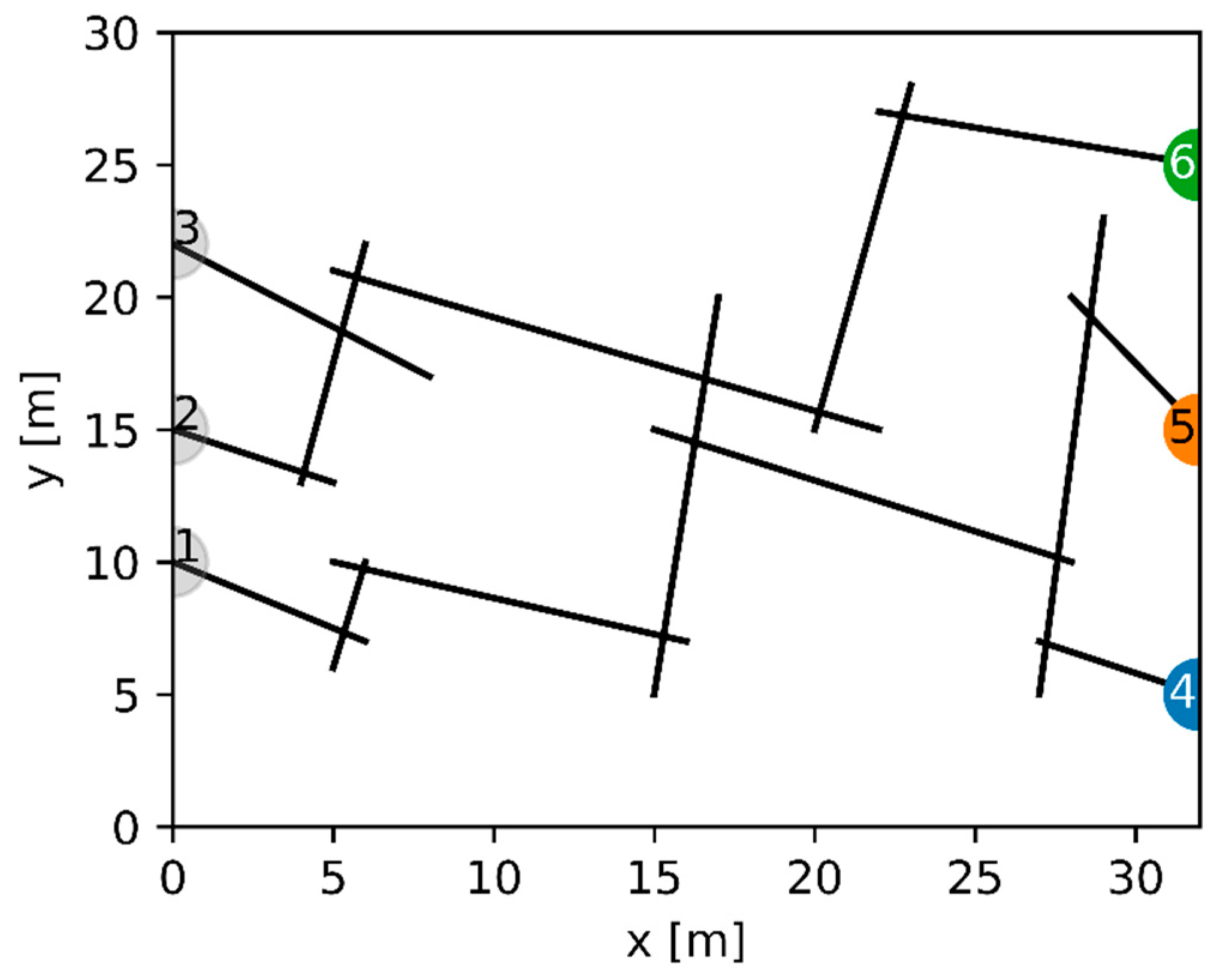
Figure 1. Synthetic discrete fracture network with three injection points (number one to three) and three receiver points (number four to six) based on an outcrop in Switzerland. It contains two fracture sets with two different fracture angles and fracture apertures.
Geosciences 09 00274 g001
Figure 2. Flowchart showing the inversion algorithm with its main phases.
Geosciences 09 00274 g002
Figure 3. Scheme to explain the procedure of drawing samples from a variance posterior probability density function (pdf).
Geosciences 09 00274 g003
Figure 4. (a) Synthetic discrete fracture networks (DFN) and (b) the results using the pressure signals for the inversion illustrated as fracture probability map.
Geosciences 09 00274 g004
Figure 5. (a) Synthetic DFN and (b) the results using the tracer breakthrough curves for the inversion illustrated as fracture probability map.
Geosciences 09 00274 g005
Figure 6. Noisy tracer breakthrough curves ( σ n o i s e = 3 ) for different combinations of source and receiver points: (a) tracer injection at source 1; (b) tracer injection at source 2; and, (c) tracer injection at source 3. The colors of the graphs accord with the colors of the receiver points in Figure 1.
Geosciences 09 00274 g006
Figure 7. Histogram of variance samples during the inversion and posterior pdf of σ n o i s e 2 p ( σ n o i s e 2 | ξ o b s ,   θ σ n o i s e 2 ) in the last iteration of the rjMCMC loop (a) inversion of σ n o i s e 2 using the inverse gamma prior; and, (b) inversion of σ n o i s e 2 using the uniform prior.
Geosciences 09 00274 g007
Figure 8. Noisy pressure signals ( σ n o i s e = 3000 ) for different combinations of source and receiver points: (a) water injection at source 1; (b) water injection at source 2; (c) water injection at source 3. The colors of the graphs accord with the colors of the receiver points in Figure 1.
Geosciences 09 00274 g008
Figure 9. Histogram of variance samples and posterior pdf of σ n o i s e 2 in the last step of the inversion.
Geosciences 09 00274 g009
Table 1. List of geometric constraints, experimental and inversion parameter settings (FLD: fracture length distribution).
CategoryParameterFracture Set #1Fracture Set #2
Geometric constraintsFracture inclination (°)−19.4874.48
Fracture aperture (mm)1.51
FLD-mean (m)9.9
FLD-variance m28.5
Experimental parameter settingsInjection pressure (Pa)3 × 10⁵
Injection concentration (mg/l)40
Inversion parameter settingsDiscretization length (m)1
p a d d / p d e l / p s h i f t 0.4/0.4/0.2
Number of rjMCMC iterations100,000