Evaluation of Different Pooling Methods to Establish a Multi-Century δ¹⁸O Chronology for Paleoclimate Reconstruction

Abstract

To develop multi-century stable isotope chronologies from tree rings, pooling techniques are applied to reduce laboratory costs and time. However, pooling of wood samples from different trees may have adverse effects on the signal amplitude in the final isotope chronology. We tested different pooling approaches to identify the method that is most cost-efficient, without compromising the ability of the final chronology to reflect long-term climate variability as well as climatic extreme years. As test material, we used δ¹⁸O data from juniper trees (Juniperus polycarpus) from Northern Iran. We compared inter-tree and shifted 5-year blocks serial pooling of stable isotope series from 5 individual trees and addition of one single series to a shifted serial pooled chronology. The inter-tree pooled chronology showed the strongest climate sensitivity and most synchronous δ¹⁸O variations with the individual tree ring analyses, while the shifted block chronologies showed a marked decline in high-frequency signals and no correlations with climate variables of the growth year. Combinations of block-pooled and single isotope series compensated the high-frequency decline but added tree-individual climatic signals. Therefore, we recommend pooling calendar synchronous tree rings from individual trees as a viable alternative to individual-tree isotope measurements for robust paleoclimate reconstructions.

1. Introduction

Among the various tree-ring parameters used to investigate long-term climate variability and reconstruct past climate conditions, variations of stable isotopes in tree-ring cellulose offer the great advantage of preserving low-frequency climate signals [1,2,3,4,5,6]. Tree-ring stable isotopes are less affected by age-related non-climatic factors [7,8]. Unlike variations in tree-ring width (TRW), tree-ring δ¹⁸O potentially records climate or environmental signals, even when there is no dominant climatic control on tree growth at a site, which is often the case in regions where not one single climate factor limits tree growth [7,9,10,11,12].

With the development of online techniques and other innovations, stable isotopes analysis became more cost efficient and faster [4,13,14,15,16,17,18,19,20]. Nevertheless, the analysis of stable isotope ratios in annually resolved tree rings is still a time consuming as well as a labor and cost intensive process. This holds especially true when one is aiming to establish well-replicated multi-centennial to millennial stable isotope chronologies composed of a larger number of living and subfossil trees [21]. As an important precondition, the construction of a reliable stable isotope chronology requires a sufficient sample replication to obtain a precise average isotope chronology that represents a representative signal for a study site that can reflect a characteristic climatic signal for that region. Several studies suggest that 4 to 6 trees are sufficient to establish a reliable local isotope chronology providing a representative site signal for climate reconstruction [22,23,24,25,26].

Combining several cross-dated tree rings of identical age from different tree individuals prior to isotopic analysis is one of the techniques providing the possibility of increasing the replication of an isotope chronology without increasing the number of isotope analyses [14] (thereafter referred as “pooling”). Furthermore, pooling enables the establishment and the extension of isotope chronologies further back in time at lower cost. Hence, the pooling technique has been widely used for valuable paleoclimate reconstructions [21,27,28,29,30,31,32,33,34,35,36,37,38,39]. Various techniques exist for pooling tree rings prior to stable isotope analysis such as (i) inter-tree pooling, which combines calendar synchronous tree rings from individual trees [15,22,40,41]; and (ii) serial pooling, which combines the use of pentad or temporally lower resolved blocks within the individual trees, with the risk of losing high-frequency climate signals [14]. Development of different pooling techniques is a sustainable benefit to stable isotope dendroclimatology by reducing sample preparation time and cost. However, the resulting isotope chronologies might contain some bias due to (i) unweighted pooling of different masses of individual tree rings; (ii) including trees containing individual disturbance signals with poor correlation to the rest of the population; (iii) uncertainties associated with sample handling and statistical properties of the resulting time series, i.e., sample preparation, analytical process, and autocorrelation of the final chronology.

With regard to the great advantages of the pooling methods when it comes to saving time and costs, several studies attempted to rectify the possible methodological errors and improve the efficiency of pooling methods by utilizing new strategies in combining tree rings series. Boettger and Friedrich [14] developed a serial pooling method which combines the advantages of ‘serial’ and ‘inter-tree’ pooling for constructing isotope chronologies with annual resolution. This method is particularly recommended for the establishment of long multi-replicated supra-regional isotope chronologies, especially in the case of tree species forming extremely narrow tree rings [32]. Gagen et al. [17] were able to establish a millennial length tree-ring δ¹³C chronology using an “offset-pool plus Joint-Point” method. This approach offers the possibility to efficiently combine a large sample replication to quantify uncertainty estimates with the possibility to preserve low frequency signals. However, the quality and quantity of available resources and the main interest of study are decisive factors in selecting a sampling strategy. In a recent study, Haupt et al. [19] assumed the availability of only five trees for stable isotope analyses and evaluated the shifted 5-year serial block pooling technique, testing if the resulting mean chronology is representative for the site and allows climate reconstruction. They suggested combining five series of shifted 5-year blocks with one additional series at annual resolution, thereby significantly improving the variance of the final chronology and allowing the reconstruction of both, long-term climate variations and extreme years.

The motivation for the present study is to establish a well-replicated multi-century δ¹⁸O chronology for Northern Iran, an area where to date paleoclimate information derived from dendrochronology has been sparse. Since the final chronology will be composed of various individual trees of different age, we tested different pooling approaches to minimize analysis costs without compromising the ability of the final chronology to reflect long-term climate variability as well as climatic extreme years. We evaluated the properties of differently pooled chronologies and annually resolved mean stable isotope chronologies from individual trees to determine the most reliable alternate pooling technique for individual analysis of tree rings. In this study, we assess the optimization effect of adding one additional stable isotope series with annual resolution on a chronology derived by shifted 5-year block pooling. The target is to obtain the chronology which best represents isotope variations of the site and contains the strongest climate signal, but on the other hand offers the best combination of time and cost efficiency.

2. Material and Methods

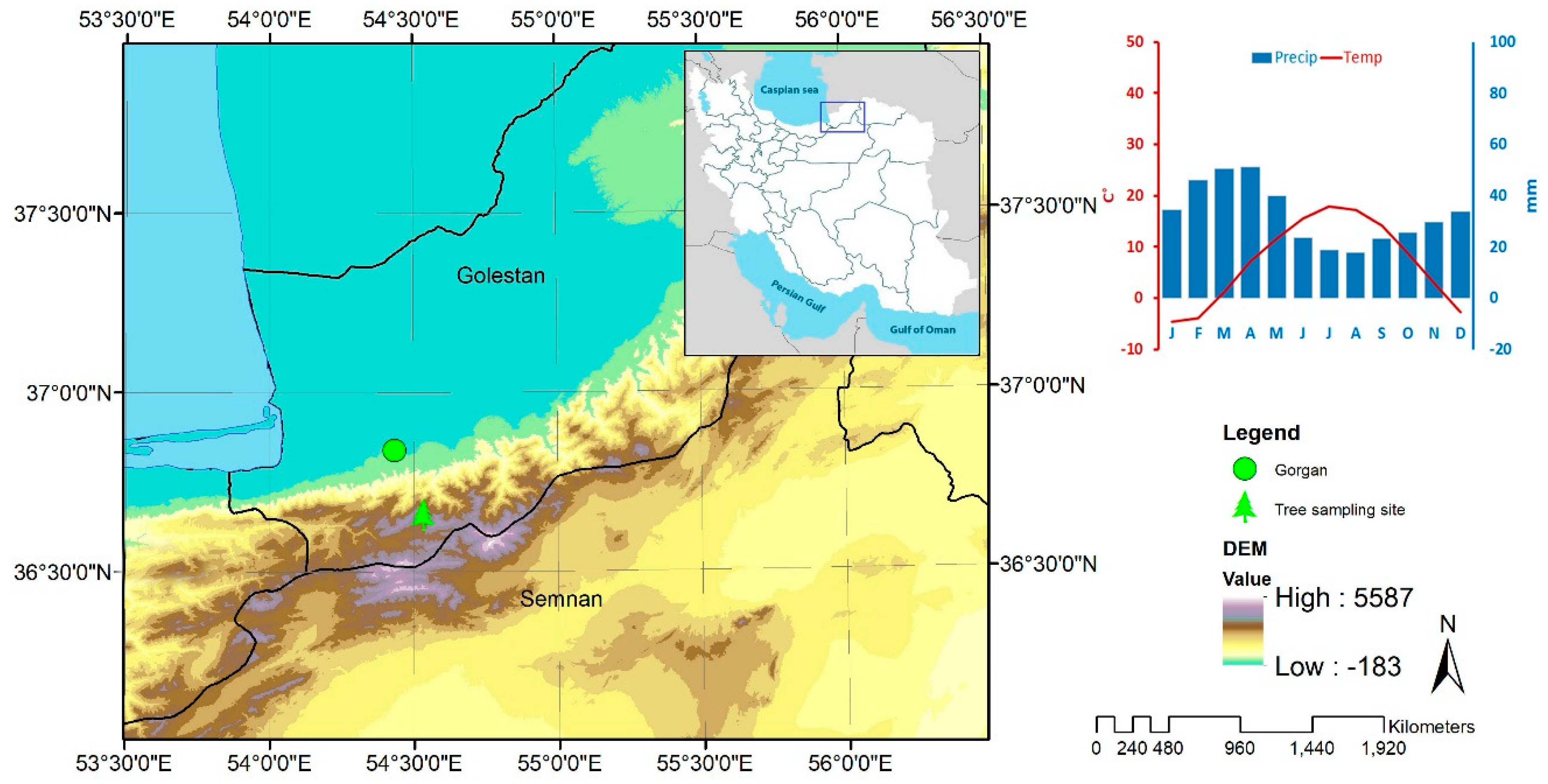
2.1. Study Site and Climate Data

As characterized by Pourtahmasi et al. [42,43], Juniperus polycarpus is a long-living drought and cold-tolerant tree species resistant to the harsh mountain climate conditions in the southern slopes of the Alborz Mountains in North Iran. Because of its high tree ages of more than 500 years, it is widely used for dendroclimatology studies in Northern Iran [43,44,45]. We sampled tree-ring material from high-elevation and open forests of J. polycarpus (36°39′54, 4″ N; 54°31′53, 7″ E) near the village Chahar Bagh situated on the south-facing slope of the Alborz Mountains at an elevation of 2540 m a.s.l [46,47] (Figure 1). Regional climate is characterized by cold and long winters and dry summers, with mean annual temperatures and total precipitation of 7 °C and 394 mm, respectively [48]. Precipitation mainly occurs in late autumn, winter, and early spring. The summer is arid, hot and sunny, with intensive radiation most of the time.

Due to the lack of local meteorological data at the study site for calibrating tree-ring δ¹⁸O -climate relationships, we used meteorological data modeled by Nadi et al. [48]. They applied interpolation methods using the meteorological data of Gorgan climate station (36°51′ N; 54°16′ E; 13.3 m a.s.l., 1958–2007) (Figure 1) as input variables and used 3D linear gradient and linear and nonlinear hybrid methods based on regional lapse rates to model temperature and precipitation at our study site (36°46′ N; 54°65′ E; 2000 m a.s.l.; Figure 1) [48].

2.2. Tree-Ring Material

Two increment cores per tree were sampled from a total of 57 juniper trees using increment borers with 5 mm diameter. Tree-ring widths of the total 114 samples were measured with a LINTAB 5 table (Rinntech, Germany) at a resolution of 0.01 mm. Tree-ring series were statistically and visually cross-dated following standard procedures [49], including using the TSAP software. In a next step, we selected 5 of the 57 trees for further processing using pooled stable isotope analysis. To ensure that the selected trees represent the common growth signal, we selected trees that had no missing rings and whose ring-width series showed high correlations with the mean tree-ring chronology.

Insufficient amount of material of individual tree rings is a common problem of stable isotope dendroclimatology, which can be caused by rotten or damaged wood and extremely narrow tree rings, especially in very old tree individuals. Employing pooling techniques helps to overcome this inherent limitation. However, there are challenges to interrogate pooling methods about their efficiency. For instance, while the mean isotope chronology constructed by inter-tree pooling is more similar to mean isotope series assessed by individually analyzing the tree rings, serial pooling undermines the great advantage of annual resolution of tree rings. In doing so, isotope signals captured by serial pooling reflect long-term variations/frequencies rather than short-term variations or extreme events [14,19].

Another challenge of pooling tree rings concern uncertainties associated with the statistical properties of the final isotope chronology. To obtain a representative mean isotope value for all trees from a study site, the aim must be to retain as much of the common signal as possible. The largest source of variability in stable isotope ratios of tree ring cellulose is the difference in the mean isotope fractionation level among individual trees. These differences can result in variance that is not common between trees of the same region (‘noise’) and may be caused by genetic factors, individual environmental disturbances or microsite conditions. Inter-tree pooling presents a single representative annual value for each year and thereby enables calculations of important characteristics of the resulting isotope chronology, such as like inter-annual variability, autocorrelation, and other variables [15,16].

A number of studies have already evaluated the problem of inter-tree variability and its contribution to error of pooling without regard to mass [13,15,41,50,51]. In most cases, the results indicated that the inter-tree pooling of tree rings regardless of their individual mass provides the same mean chronology as ones calculated from individual analyses of tree rings. However, the combination of unweighted rings from a rather small number of different trees showing different first-order autocorrelation might bias the time series characteristics of the final isotope chronology [15,16].

2.3. Pooling Strategies for Tree-Ring Isotope Samples

In order to assess the most suitable pooling technique, we applied inter-tree pooling (ITP) and serial pooling of shifted five-year blocks (SBP). Both methods significantly reduce the required number of isotopic measurements and α-cellulose extractions compared to individual tree ring analyses. However inter-tree pooling still demands the same effort in sample preparation and the accurate manual separation of the individual tree rings from which may incur problems through the mixing of wood material from neighboring tree rings [22,24,28,39].

According to our study design, one core per tree of the five sample trees was used for inter-tree pooling and another core for serial pooling of shifted 5-year blocks. The two methods differ in terms of their pattern of cutting and pooling the tree rings. For ITP, individual tree rings of 5 trees for the 50-year period 1958 to 2007 were carefully separated. Prior to cellulose extraction, the annually resolved wood material of calendar synchronous tree rings of 5 trees was pooled without regard to the mass of each ring (Figure 2a).

For SBP, each core was split into blocks of five consecutive tree rings. Between the five sampled trees, these pentad blocks were shifted by one year in calendar position (Figure 2b).

The splitting procedures for both groups of samples were carried out under a binocular microscope with a razor blade. Consecutively, each of the samples was cut into smaller pieces and encapsulated into an Eppendorf vial for α-cellulose extraction. Further pre-IRMS treatments such as cellulose extraction were conducted identically for both groups of samples.

2.4. Stable Isotope Measurements

The α-cellulose was extracted following the three-step method described by Wieloch et al. [52]: (i) removal of the minor components like resins and hemicellulose using NaOH 5% (pretreatment); (ii) delignification with a 7% NaClO₂ solution; (bleaching); and, (iii) elimination of non-α-cellulose compounds with NaOH (17%) in the alkaline hydrolysis step (cellulose purification). The cellulose samples of each calendar year and pentad block was homogenized by ultrasonic homogenization [53] followed by freeze drying.

The stable oxygen isotopes ratios of α-cellulose samples were measured online (analytical precision typically better than ± 0.25‰) using an isotope ratio mass spectrometer (Delta V Advantage, Thermo Fisher Scientific Inc.) coupled to a high temperature (1450 °C) pyrolysis reactor (HEKATECH). The oxygen values are expressed as δ¹⁸O in per mil (as ‰) relative to the international VSMOW standard (VSMOW, Vienna Standard Mean Ocean Water). The annually resolved stable oxygen isotope series (chronology A) established from the individual analyses had been measured by Foroozan et al. [54].

2.5. Constructing Pooling Chronologies

To obtain a SBP, shifted five-year-block series of each chosen core were averaged. The annual mean δ¹⁸O values were calculated by three averaging methods; (i) a 5-year running mean calculation of the δ¹⁸O values with one year offset among δ¹⁸O series for each annual δ¹⁸O values (chronology was labelled SBP_r), as illustrated in Figure 3a, (ii) arithmetic mean from averaging individual tree-ring δ¹⁸O values of the δ¹⁸O series (labelled SBP_a), as shown in Figure 3b; (iii) transforming each shifted pentad block δ¹⁸O series into standardized score (z-scores) and calculating the mean isotope SBP_z series at annual resolution (labelled SBP_z).

To test the influence of a single individual isotope series on the shifted 5-year block serial pooled mean series, we selected δ¹⁸O series of three different juniper trees that showed the strongest correlations with the mean annually resolved δ¹⁸O chronology A (named J₁, J₂ and J₃). In a next step, the new chronologies were built by combining each of the additional series with annual resolution with SBP_r (chronologies were labelled SBP_rJ₁, SBP_rJ₂, and SBP_rJ₃), SBP_a (labelled SBP_aJ₁, SBP_aJ₂, and SBP_aJ₃) and SBP_z (labelled SBP_zJ₁, SBP_zJ₂, and SBP_zJ₃). Furthermore, to evaluate the suitability of the additional annual resolved series, we reduced the impact of individual series to only 25% in combining it with shifted 5-year block chronologies SBP_r (labelled SBP_rJ_125%, SBP_rJ_225%, and SBP_rJ_325%), SBP_a (labelled SBP_aJ_125%, SBP_aJ_225%, and SBP_aJ_325%), SBP_z (labelled SBP_zJ_125%, SBP_zJ_225%, and SBP_zJ_325%) (Table S1).

In order to evaluate the resulting mean chronologies of different pooling methods, we applied the following procedures: i) we assessed time-series characteristics and the ability to capture extreme climatic events using the mean, standard deviation (SD), the range of maximum and minimum values of δ¹⁸O data series (Figure 4), normality of value distribution, autocorrelation (

Table 1. Statistical characteristics of the individual and mean δ¹⁸O data series: first and second order autocorrelation (AC1 and AC2); normal distribution tests: skewness, Kurtosis, and Shapiro–Wilk test.

		AC1	AC2	Skewness	Kurtosis	Shapiro–Wilk
Individual analyses	Juniper1	0.37 **	0.06	−0.52	−0.29	0.08
	Juniper2	0.21	0.29	0.54	0.15	0.43
	Juniper3	0.16	0.13	−0.04	0.37	0.59
	A	0.26	0.06	0.2	−0.52	0.42
Pooling	ITP	0.38 **	0.08	−0.29	−0.09	0.86
	SBPr	0.69 **	0.50 **	−0.52	0.75	0.65
	SBPrJ1	0.45 **	0.11	−0.66	−0.16	0.01
	SBPrJ2	0.40 **	0.37 *	0.67	0.06	0.15
	SBPrJ3	0.25	0.17	0.23	0.20	0.56
	SBPrJ125%	0.60 **	0.27	−0.64	−0.28	0.04
	SBPrJ225%	0.61 **	0.48 **	0.36	−0.69	0.23
	SBPrJ325%	0.47 **	0.37 *	0.33	−0.20	0.66
	SBPa	0.87 **	0.68 **	0.17	0.01	0.41
	SBPaJ1	0.49 **	0.15	−0.60	−0.10	0.01
	SBPaJ2	0.49 **	0.41 **	0.60	0.15	0.22
	SBPaJ3	0.38 *	0.25	0.24	0.10	0.67
	SBPaJ125%	0.67 **	0.38 *	−0.46	−0.18	0.23
	SBPaJ225%	0.71 **	0.56 **	0.45	−0.04	0.24
	SBPaJ325%	0.64 **	0.45 **	0.34	−0.12	0.49
	SBPz	0.83 **	0.6 **	−0.04	0.10	0.72
	SBPzJ1	0.58 **	0.29 *	−0.50	−0.41	0.03
	SBPzJ2	0.54 **	0.44 **	0.34	0.10	0.88
	SBPzJ3	0.55 **	0.37 **	0.39	−0.08	0.35
	SBPzJ125%	0.75 **	0.49 **	−0.33	−0.27	0.52
	SBPzJ225%	0.73 **	0.55 **	0.08	−0.01	0.83
	SBPzJ325%	0.74 **	0.51 **	0.23	−0.40	0.22

Double and single asterisks indicate significant correlations at the p-value < 0.05 and p-value < 0.01 levels, respectively.

) and Kruskal–Wallis test (Table S2). Then, we evaluated the degree of correspondence of inter-annual variations between different versions of isotope chronologies using correlation analysis (Figure 5 and Figure 6).

The annually resolved δ¹⁸O chronology obtained from individual analyses (chronology A) was taken as reference chronology for comparison with all different pooled chronologies. To reveal differences in recorded climate signals of the different isotope chronologies, we calculated Pearson’s correlation coefficients with the climate parameters temperature and precipitation (Figure 7 and

Table 2. Significant climate- δ¹⁸O correlation of various chronologies during current year.

Precipitation					Temperature
	Apr	May	Winter	Spring		Jan	Feb	Mar	Apr	May	Winter	Spring
A	–0.44 *	–0.59 **	–0.39 *	–0.59 **	A	0.50 **			0.42 *	0.45 *	0.45 *	0.50 *
ITP		–0.51 **	–0.42 *	–0.47 *	ITP	0.49 *	0.46 *				0.53 **	0.42 *
SBPr					SBPr
SBPrJ1		–0.66 **		–0.60 **	SBPrJ1	0.48 *				0.53 *
SBPrJ2					SBPrJ2		0.45 *			0.52 *	0.46 *	0.50 *
SBPrJ3					SBPrJ3
SBPrJ125%		–0.58 **		–0.52 *	SBPrJ125%	0.46 *				0.46 *	0.43 *
SBPrJ225%					SBPrJ225%		0.45 *				0.46 *
SBPrJ325%					SBPrJ325%
SBPa					SBPa
SBPaJ1		–0.67 **		–0.61 **	SBPaJ1	0.49 *				0.55 **	0.44 *
SBPaJ2				–0.43 *	SBPaJ2		0.44 *		0.44 *	0.54 *	0.47 *	0.52 *
SBPaJ3					SBPaJ3
SBPaJ125%		–0.59 **		–0.54 *	SBPaJ125%	0.45 *				0.51 *	0.46 *
SBPaJ225%					SBPaJ225%			0.44 *		0.49 *	0.48 *	0.46 *
SBPaJ325%					SBPaJ325%			0.43 *
SBPz					SBPz
SBPzJ1		–0.57 **		–0.50 *	SBPzJ1	0.53 **					0.46 *
SBPzJ2					SBPzJ2			0.43 *			0.46 *
SBPzJ3					SBPzJ3			0.42 *
SBPzJ125%		–0.46 *		–0.41 *	SBPzJ125%	0.45 *					0.44 *
SBPzJ225%					SBPzJ225%			0.43 *			0.44 *
SBPzJ325%					SBPzJ325%			0.40 *

Double and single asterisks indicate significant correlations at the p-value < 0.05 and p-value < 0.01 levels, respectively.

and

Table 3. Significant climate- δ¹⁸O correlation of various chronologies during the previous year.

	Precipitation								Temperature
	Py Mar	Py Apr	Py May	Py Aug	Py Sep	Py Spring	Py Summer		Py Jan	Py Feb	PMar	Py May	Py Sep	Py Winter	Py Spring
A	–0.40 *	–0.37	–0.53 **			–0.52 **		A
ITP	–0.40 *		–0.55 **		0.42 *	–0.52 **		ITP
SBPr			–0.57 **	0.50 *		–0.50 *	0.48 *	SBPr	0.46 *					0.51 *
SBPrJ1	–0.53 *		–0.64 **	0.45 *		–0.60 **		SBPrJ1
SBPrJ2				0.49 *	0.44 *		0.57 **	SBPrJ2			0.58 **		0.45 *	0.50 *
SBPrJ3	–0.52 *		–0.50 *		0.47 *	–0.51 *		SBPrJ3						0.46 *
SBPrJ225%	–0.49 *		–0.66 **	0.50 *		–0.61 **	0.48 *	SBPrJ225%
SBPrJ225%			–0.50 *	0.540 *	0.46 *		0.59 **	SBPrJ225%	0.46 *		0.57 **			0.55 **
SBPrJ325%	–0.46 *		–0.56 **		0.46 *	–0.53 *	0.46 *	SBPrJ325%	0.46 *	0.44 *				0.51 *
SBPa	–0.44 *		–0.60 **	0.60 **	0.47 *	–0.58 **	0.63 **	SBPa			0.46 *	0.51 *		0.48 *	0.49 *
SBPaJ1	–0.55 **		–0.65 **	0.49 *		–0.62 **	0.48 *	SBPaJ1
SBPaJ2			–0.43 *	0.52 *	0.46 *		0.61 **	SBPaJ2			0.58 **		0.45 *	0.49 *
SBPaJ3	–0.56 **		–0.55 **		0.50 *	–0.56 **	0.50 *	SBPaJ3			0.44 *	0.50 *		0.49 *	0.52 *
SBPaJ125%	–0.54 *	–0.43 *	–0.67 **	0.55 **		–0.64 **	0.56 **	SBPaJ125%
SBPaJ225%			–0.53 *	0.58 **	0.49 *	–0.49 *	0.65 **	SBPaJ225%			0.56 **			0.51 *	0.46 *
SBPaJ325%	–0.53 *		–0.59 **	0.49 *	0.51 *	–0.59 **	0.57 **	SBPaJ325%			0.46 *	0.52 *		0.51 *	0.52 *
SBPz			–0.52 **	0.47 *		–0.41 *	0.51 **	SBPz						0.41 *
SBPzJ1	–0.41 *		–0.61 **	0.43 *		–0.56 **		SBPzJ1
SBPzJ2			–0.43 *	0.44 *			0.50 *	SBPzJ2			0.41 *
SBPzJ3	–0.44 *		–0.54 **		0.47 *	–0.46 *	0.49 *	SBPzJ3	0.45 *		0.43 *			0.50 *
SBPzJ125%			–0.59 **	0.48 *		–0.52 **	0.47 *	SBPzJ125%
SBPzJ225%			–0.49 *	0.48 *			0.52 **	SBPzJ225%						0.41 *
SBPzJ325%			–0.53 **	0.44 *	0.41 *	–0.44 *	0.50 *	SBPzJ325%	0.42 *					0.45 *

).

3. Results and Discussion

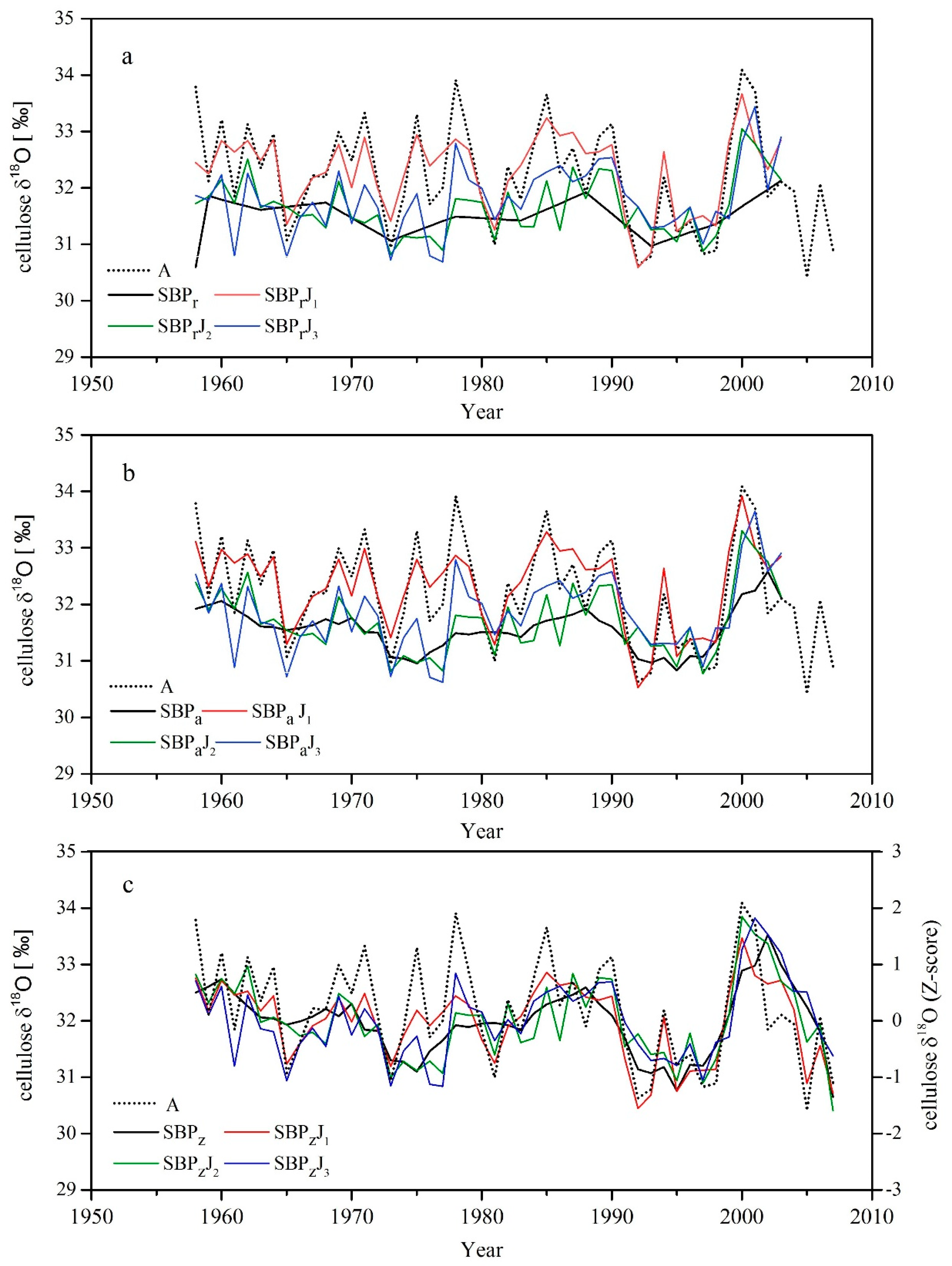
3.1. δ¹⁸O Variations among Different Individual and Pooled Chronologies

The statistical results for the three individual isotope series (juniper 1, 2, and 3), and the mean chronology derived from 5 individual δ¹⁸O series (A) and pooled chronologies are presented in Figure 4.

The mean of the inter-tree pooled δ¹⁸O series ITP (mean = 31.88‰) shows only subtle differences compared to the δ¹⁸O chronology averaged from individual tree series (A; mean = 32.11‰), followed by SBPa (mean = 31.56‰) and SBPr (mean = 31.49‰), respectively (Figure 4).

A visual comparison of the patterns of inter-annual variations of δ¹⁸O values in “A”, serial (SBPr, SBPa, SBPz) and inter-tree pooled chronologies are shown in Figure 5. Inter-annual variability of δ¹⁸O in the inter-tree pooled chronology (SD = ±0.82, range = 3.93) is higher than that of the serial pooled chronologies (${\mathrm{SD}}_{\mathrm{SBPr}}$ = ±0.29, ${\mathrm{range}}_{\mathrm{SBPr}}$ = 1.54; ${\mathrm{SD}}_{\mathrm{SBPa}}$ = ±0.38, ${\mathrm{range}}_{\mathrm{SBPa}}$ = 1.74). As expected the smoothed shifted 5-year block serial pooled series conserves a lower amount of high-frequency signals and consequently extreme events, with the exception of SBP_z (${\mathrm{SD}}_{\mathrm{SBPz}}$ = −0.02 ± 0.6, ${\mathrm{range}}_{\mathrm{SBPz}}$ = 2.88). Our results confirm the findings of Boettger and Friedrich [14] of smaller standard deviations and highly damped high frequency signals for the shifted five-year blocks data.

All δ¹⁸O series measured on pool show similarities with “A”, especially during common minimum years (1991–1996 (except SBP_r), 1965, 1974, and 1983) (Figure 5). Inter-tree pooled chronology shows higher synchronism of inter-annual variations with the chronology A, especially during 1981–1999. Nonetheless, there are differences among chronologies in individual years, for instance a rapid increase of δ¹⁸O values in 1970 was observed in pooled chronologies, while in same year chronology A shows declining values. Besides, several events do not coincide between chronologies.

When comparing δ¹⁸O chronologies derived from pooled and individual tree rings at two locations from the Iberian Peninsula, Dorado Liñán et al. [15] found a generally good agreement between inter-tree pooled chronologies and the mean series of individual values. They cautioned that the mean δ¹⁸O values for pooled and averaged values of the mean master series differed by 0.25‰ and 0.36‰ in two study sites, while SD was similar among the two types of isotope series. In the present study, mean differences between “ITP” and “A” are substantially lower (0.02‰), with a high degree of variability and standard deviation highly similar to “A” (Figure 4 and Figure 5).

For the purpose of saving time and effort in sample preparation, inter-pooling of the tree rings was done regardless of the mass contribution of each tree ring [13,16,22,26,41]. In compliance with Szymczak et al. [4], the features reflected in the inter-tree pooled chronology confirm that pooling without considering different contributions of the single trees produces a reliable isotope chronology which does not suffer from error associated with unequal mass contributions of individual tree rings.

The correlations between different δ¹⁸O chronologies are shown in Figure 6. Pearson correlation coefficients between pooled and individual chronologies confirmed that all variants of chronologies were significantly correlated to at least one other chronology version. Significant correlations among all chronologies reveal common variance between the pooled δ¹⁸O series and the annually resolved chronology A. The correlations tended to be higher between inter-annual variations of the inter-tree pooled “ITP” and the “A” chronologies (${\mathrm{r}}_{\mathrm{ITP}/\mathrm{A}}$ = 0.86; p < 0.01) and much lower but still significant between the shifted 5-year block series and the A chronology (${\mathrm{r}}_{\mathrm{SBPr}/\mathrm{A}}$ = 0.46, ${\mathrm{r}}_{\mathrm{SBPa}/\mathrm{A}}$ = 0.55, ${\mathrm{r}}_{\mathrm{SBPz}/\mathrm{A}}$ = 0.56; p < 0.01) [14,19]. This underlines the higher degree of agreement and the highly synchronous isotope signal in the annually resolved inter-tree pooled series and chronology A.

Treydte et al. [51] reported highly significant correlations of 0.85 between pool-individual chronologies from juniper tree-ring cellulose from northern Pakistan, which is in agreement with our result. However, studies by Dorado Liñán et al. [15] and Szymczak et al. [4] conducted from conifer species from different regions have shown lower pool-individual chronologies correlations of approximately 0.66.

Autocorrelations of annually resolved δ¹⁸O series (J₁, J₂, J₃, and A) and pooled chronologies showed that among annually resolved δ¹⁸O series obtained from the individual analyses, only the first-order autocorrelation of J1 (AC1 = 0.37, p < 0.01) is significant (Table 1).

Differences in autocorrelation among single δ¹⁸O series can emanate from water resource availability for individual trees [15,55]. The evergreen juniper has a shallow root system and roots lie close to the soil surface and use internally stored and superficial soil water supplies [56,57]. However, some trees with deeper root systems may use winter recharge or ground water stored in the soil for more than one growing season [55,58,59]. Furthermore, trees growing under different individual micro-site conditions can use water after snow melt in spring for wood formation in the early growing season. Beside, conducting stable isotope measurements of total tree rings may obscure seasonal climate fluctuations by mixing the signals registered in earlywood and latewood [24]. Isotope signals in earlywood are associated with isotope values of the previous year as a result of using stored carbohydrates from the previous year and mixing them with current year photosynthetic products for earlywood formation at the beginning of the growing season. These memory effects of preceding years on the isotope signal [13,17] can be reduced by separating earlywood from late wood and investigating the stable isotope signal only in the latewood of the tree ring [60,61]. On the other hand, Kress et al. [62] found high common isotope signals between earlywood and latewood in European tree-line conifers, suggesting that the separation of earlywood from latewood is unnecessary. They assumed that high turnover rates and limited reserve storage in the investigated species prevent the mobilization of carbohydrate reserves formed in the previous year. Hence, they recommended the use of whole-ring cellulose to record the annual isotopic signal from conifer tree-ring stable isotopes. Given the narrow tree rings of junipers and their small latewood portion of the tree ring, we used the whole tree rings for isotope measurements [4,28].

For pooled chronologies, except for the inter-tree pooled chronology ITP which shows only a significant first-order autocorrelation (AC1 = 0.38, p < 0.01) [15], the first and second-order autocorrelations of all shifted 5-year block series (SBP_r, SBP_a, and SBP_z) are significant (Table 1). These considerations adumbrate the actual climate signal and the independence of the current year’s growth from the previous year’s influence.

3.2. Correlations between Isotope Chronologies and Climate Parameters

Correlation analysis between isotope chronologies and climate data of individual months and seasons of the current and previous year indicated the most common significant relationships with May and spring precipitation in all chronologies (Figure 7). For further discussion, we therefore focused on precipitation-proxy correlations during spring and May (Table 2 and Table 3).

For chronology A, highest climate-proxy correlations are found with May precipitation (r_M = −0.59; p < 0.01) and spring precipitation (April-June; r = −0.59; p < 0.01) during the vegetation period which last from the beginning of April until the beginning of October [44] (Figure 7a, Table 2). Δ¹⁸O values have a significant positive correlation with temperatures in different months and seasons, e.g., with January and May and winter and spring [54] (Figure 7c, Table 2). Several tree-ring stable isotope studies have found similar climate- δ¹⁸O relationships, like in Asian juniper species growing on the Tibetan Plateau [28,32,39,63].

The Inter-tree pooled chronology (ITP) (r_MAY = −0.51; p < 0.01) showed higher similarities in captured climate signals with the annual resolved chronology A during the current growing season, as both chronologies have significant negative correlations with May and spring precipitation of the current year (Figure 7a, Table 2).

The correlation of temperatures and δ¹⁸O showed consistency between different chronologies. The strength of the positive correlations between the ITP mean series and spring temperature of the current year was weaker compared to series A, but still highly significant (Figure 7c, Table 2). No significant correlations between shifted 5-year block series (SBP_r, SBP_a, and SBP_z) were found with total precipitation and average temperatures of any month or seasonal average during the current year of growth (Figure 7a,c, Table 2).

In general, δ¹⁸O of tree-ring cellulose reflects the isotopic composition of source water (local precipitation or ground water) and the degree of evaporative enrichment in the leaves [64]. Climate signals registered in tree-ring oxygen isotope ratios are the result of direct effects of temperature on the isotopic composition of precipitation (source water) and the dominant control of vapor pressure (air humidity) on evaporative enrichment on the leaf level [59,65]. The observed climate-proxy relationships reported in this study confirmed that juniper δ¹⁸O on the southern slopes of the mountainous areas of North Iran is mainly controlled by the level of δ¹⁸O enrichment occurring in the leaf. The strong negative and positive correlations between juniper δ¹⁸O and precipitation and temperatures, respectively, during the growing season indicate the combined effect of spring temperatures and precipitation on evaporative enrichment by controlling vapor pressure deficit in the atmosphere. Accordingly, higher precipitation amounts in the early growing season are associated with higher vapor pressure, resulting in reduced evapotranspiration and δ¹⁸O enrichment in leaf water, and consequently lower δ¹⁸O_TRC [28,63,66]. Since vapor pressure or relative humidity data are not available, we considered precipitation amounts and temperatures in spring as a surrogates to represent moisture conditions, as described by Foroozan et al. [54].

The significant correlation coefficients between δ¹⁸O chronologies and average monthly and seasonal precipitation and temperature of the previous year are documented in Figure 7b,d, and Table 3. Shifted 5-year block series (SBP_r, SBP_a, and SBP_z), which so far showed no significant correlations with climate parameters in the current year, along with other pooled chronologies show highly significant correlations with climate parameters of the previous year. These correlations correspond to the significant first and second-order autocorrelations of the shifted 5-year block chronologies. We assumed mixing consecutive tree rings may maximize the influence of preceding years and consequently minimize the climatic signal of the current year.

While series A is strongly correlated to precipitation of May (r_{py May} = −0.53; p < 0.01) and spring season (r_{py Spring} = -−0.52; p < 0.01) of the previous year, SBP_a is negatively correlated with precipitation in May (r_{py May} = −0.6; p < 0.01) and spring (April-June; r_{py Spring} = −0.58; p < 0.01). Series SBP_r, ITP, and SBP_z were significantly correlated to precipitation of May (r_{py May} = −0.57; p < 0.01; r_{py May} = −0.55; p < 0.01 r_{py May} = −0.52; p < 0.01) of the previous year, respectively.

3.3. Mixed Block-Pooling and Individual Series Chronology

To avoid loss of variance and of extreme event signals using the shifted 5-year blocks-serial pooling, we added a single isotope series obtained from the individual analyses to the shifted 5-year block series [19]. The addition of one annually resolved series increased the δ¹⁸O mean values in all the mixed chronologies of SBP_r, SBP_a, and SBP_z, even exceeding the mean δ¹⁸O value of chronology A (mean SBP_rJ₁ = 32.3; mean SBP_aJ₁ = 32.33) (Figure 4).

Furthermore, the ranges of maximum and minimum δ¹⁸O values in mixed chronologies have almost doubled (e.g. range SBP_rJ₂ = 3.40) and are correspond to those of the annually resolved chronology A. All mixed chronologies assessed higher standard deviations than 0.5, and the highest SD was found for SBP_aJ₁ and SBP_zJ₁ (SD = ±0.72), being close to the characteristics of chronology A (SD = ±0.88). Hence, adding one additional series resulted in a strongly increased high-frequency signal in all shifted 5-year block, as already reported by [19]. Adding one of the individual series of juniper trees (1, 2, or 3) had different effects on the improvement of serial pooled series (Figure 4 and Figure 8, Table 1). However, correlations between mixed chronologies (SBP_rJ₁, SBP_rJ₂, SBP_rJ₃, SBP_aJ₁, SBP_aJ₂, SBP_aJ₃, SBP_zJ₁, SBP_zJ₂, and SBP_zJ₃) and chronology A are all significant (p < 0.01) and range from 0.87 to 0.74 (Figure 6). While three chronologies mixed with J₁ are correlating with chronology A higher than 0.8, the other six mixed chronologies correlated above 0.7, respectively.

A highly significant correlation between mixed SBP_r and A (${\mathrm{r}}_{\mathrm{SBPrJ}1/\mathrm{A}}$ = 0.85, ${\mathrm{r}}_{\mathrm{SBPrJ}2/\mathrm{A}}$ = 0.75_, ${\mathrm{r}}_{\mathrm{SBPrJ}3/\mathrm{A}}$ = 0.75; p < 0.01) compared to a less significant correlation between SBP_r and A (r _SBPr/A = 0.46; p < 0.01) suggests statistical uncertainty associated with the inter-tree variability in mixed chronologies by adding variability not related to climatic forcing but to individual isotope signals (Figure 6). This problem could emerge by the disparity in SD and mean between the single δ¹⁸O series and shifted 5-year blocks. Constructing a mean chronology from isotope series with high variability between their means can bias the mean chronology towards the isotope series with the highest mean isotopic value [15]. It is a reasonable assumption that the mixed chronology tends to retain δ¹⁸O variations and the high frequency signal captured by one additional single individual isotope series. A number of studies have already shown high inter-tree variabilities in oxygen isotope ratios in tree species of other genera [1,4,15,26]. Possible sources of inter-tree variability can be related to the circumferential isotope variation, microenvironmental and tree genetic factors. Changes in various decisive environmental factors such as insolation, temperature, and moisture availability exert a strong influence over photosynthesis and transpiration and consequently influence the respective tree-ring isotope record.

In a next step, we tested the influence of adding an individual isotope series to the block pooled data by giving different weights to the added series. To account for the mass contribution to the final chronology, we weighed the added annually resolved series with only 25% and the shifted 5-year block series with 75% for producing mixed pooled chronologies. The aim was to examine the influence of adding different individual isotope series of J₁, J₂ and J₃ to obtain a representative mixed isotope chronology and a mean isotope value for the study site. The Kruskal–Wallis H test showed statistically significant differences between δ¹⁸O mean values of the mixed chronologies of SBP_r (χ² (6, N = 46) = 58.01, p = 0.00) and SBP_a (χ² (6, N = 46) = 45.74, p = 0.00) with the different sample weights (Table S2). However, z-scores of mixed chronologies did not significantly differ by treatments. Post-hoc Tu’ey’s HSD tests showed that mixed chronologies with the incorporation of J₁, whether weighted by 25% or 50% (equally weighted), had significantly (p < 0.05) different δ¹⁸O mean values from the other mixed chronologies with a mean rank δ¹⁸O values of 237.78 for SBP_rJ₁, 193.67 for SBP_rJ_125%, 231.35 for SBP_aJ₁, and 189.40 for SBP_aJ_125%. All other differences were not significant (not shown).

Numerical tests for normality revealed that all chronologies met the assumption of normally distributed variables except SBP_rJ₁, SBP_rJ_125%, SBP_aJ₁, and SBP_zJ₁. Albeit, SBP_r, SBP_a, and SBP_z were normally distributed, but their mixed chronologies with J₁ were not normally distributed. Even after running the statistical test to transform the data to the normal distribution they were quite robust to violate certain properties, including normal distribution or homogeneity of variances. Statistical analysis for the detection of skewed distributions and the Shapiro–Wilk test of normality are described in table 1.

With the incorporation of J₁, J₂, and J₃ into the shifted 5-year block series, first-order autocorrelations of all mixed chronologies were reduced but still remained significant (except SBP_rJ₃) (Table 1). However, mixed series in combination with J₁ and J₃ contained no significant second-order autocorrelation, while the J₃ series had the greatest impact on reducing autocorrelations in mixed series. Chronologies derived from SBP_z had the highest average of first-order and second-order autocorrelations (AC1 = 0.55 and AC2 = 0.37, p < 0.01) (Table 1).

We evaluated the influence of current and previous year’s climate on isotope signals in mixed chronologies. By adding J₁ to shifted 5-year block series, climate signals of precipitation during May and the spring season significantly appeared in the mixed chronologies (Table 2). The δ¹⁸O records in SBP₂J₁ showed the highest relationships with precipitation during May and the spring season (r_{SBPaJ1/May rainfall} = −0.67 and r_{SBPaJ1/spring rainfall} = 0.61; p < 0.01). Giving reduced weight to the J₁ series, climate-δ¹⁸O relationships become weaker (r_{SBPaJ125%/May rainfall} = −0.59; p < 0.01 and r_{SBPaJ125%/spring rainfall} = 0.54; p < 0.05), and the weakest relationships resulted for (r_{SBPzJ125%/May rainfall} = −0.46 and r_{SBPzJ1/spring rainfall} = 0.41; p < 0.05) (Table 2). The same effect was found by Haupt et al. [19], who proposed that high frequency signals and both temperature correlation and sensitivity coefficients increased significantly by adding one annual series by weighing it 100% to a block-pooled chronology.

However, we found no precipitation-proxy correlations in mixed chronologies in combination with J₂ and J₃ (except r_{SBPaJ3/spring rainfall} = −0.43; p < 0.05) for growth year (Table 2).

Stronger climate-proxy relationships of mixed chronologies were observed for climate signals of the preceding year. Correlations for the mixed chronologies vary depending on the added individual series (J₁, J₂, J₃). Evaluating the significant correlations of the δ¹⁸O mixed series with precipitation of May and spring of the previous year confirmed that adding a series with annual resolution to build the mixed chronology had different influences on climate-proxy correlations and may even weaken the climate-δ¹⁸O correlation. For example, adding J₁ to the shifted 5-year block series SBP_r lead to an increase in correlation for the mixed chronology of SBP_rJ₁ from (r_{SBPr/py May rainfall} = 0.57; p < 0.01) to (r_{SBPrJ1/py May rainfall} = 0.64; p < 0.01). In contrast, mixed chronologies in combination with J₂ conceal this relationship and showed no significant correlations with precipitation of May or spring of the previous year (Table 3).

We thus caution that the efficacy of mixed chronologies varies greatly with the selected additional annually resolved isotope series added to the block-pooled chronologies. The results of this study suggest that one arbitrarily selected additional δ¹⁸O series is not a reliable and adequate contribution to the pooled chronology to improve the properties of the mean isotopic signature. If the major aim of the study is to robustly assess the common climate signal at a site for climate reconstruction purposes, a mixed chronology has an increased risk of registering tree-dependent individual climatic signals.

4. Conclusions

The particular purposes for constructing a site-specific isotope chronology and the available resources are decisive factors in selecting appropriate sampling and pooling strategies [14,17,19]. This study explored the effect of various pooling methods on the statistical characteristics and climate responses of a site-specific δ¹⁸O-chronology, and the possibility of using pooled isotope chronologies for paleoclimate reconstruction in Northern Iran. Comparable to the results of other studies that used different pooling methods, such as inter-tree pooling [27,28,29] and shifted serial pooling [14,19], our pooled chronologies contained a significant climate signal. However, the linkage between δ¹⁸O_TRC and climate variables during the current year has been masked in the shifted 5-year block series, since conditions during preceding years have a strong influence on the isotope signal of these chronologies.

We also found that the mean of isotopic data from individually analyzed juniper trees arguably carry a stronger climate signal than any version of pooled chronologies [38]. Our investigation suggests that δ¹⁸O values of the pooled and single chronologies are both interpreted mainly in terms of site moisture conditions controlled by precipitation, despite of significant differences in the captured signals. This study proposes that inter-tree pooling best represents an alternative to individual-tree isotope measurements, since the resulting chronology showed the strongest climate sensitivity and synchronous δ¹⁸O variations with chronology A derived from averaging individual tree isotope series, whilst at the same time maintaining the main advantages of pooling concerning time and cost efficiency.

We suggest that serial pooling of shifted pentad blocks can be a practical and satisfactory alternative to extend a long δ¹⁸O chronology, when tree rings are extremely narrow, and/or increasing the replication of isotope measurements in a cost-effective way is the primary research interest. Besides, the shifted serial pooling approach is recommended for studies evaluating primarily low frequency signals and long-term trends in δ¹⁸O variations, while discarding high frequency signals and extreme event years.

References

1. Esper, J.; Frank, D.C.; Battipaglia, G.; Büntgen, U.; Holert, C.; Treydte, K.; Siegwolf, R.; Saurer, M. Low-frequency noise in δ13 C and δ18 O tree ring data: A case study of Pinus uncinata in the Spanish Pyrenees. Glob. Biogeochem. Cycles 2010, 24. [Google Scholar] [CrossRef]
2. Liu, X.; An, W.; Leavitt, S.W.; Wang, W.; Xu, G.; Zeng, X.; Qin, D. Recent strengthening of correlations between tree-ring δ13C and δ18O in mesic western China: Implications to climatic reconstruction and physiological responses. Glob. Planet. Chang. 2014, 113, 23–33. [Google Scholar] [CrossRef]
3. Gagen, M.; Zorita, E.; McCarroll, D.; Young, G.H.F.; Grudd, H.; Jalkanen, R.; Loader, N.J.; Robertson, I.; Kirchhefer, A. Cloud response to summer temperatures in Fennoscandia over the last thousand years. Geophys. Res. Lett. 2011, 38. [Google Scholar] [CrossRef] [Green Version]
4. Szymczak, S.; Joachimski, M.M.; Bräuning, A.; Hetzer, T.; Kuhlemann, J. Are pooled tree ring δ13C and δ18O series reliable climate archives—A case study of Pinus nigra spp. laricio (Corsica/France). Chem. Geol. 2012, 308–309, 40–49. [Google Scholar] [CrossRef]
5. Frank, D.C.; Poulter, B.; Saurer, M.; Esper, J.; Huntingford, C.; HELLE, G.; Treydte, K.; Zimmermann, N.E.; SCHLESER, G.H.; Ahlström, A.; et al. Water-use efficiency and transpiration across European forests during the Anthropocene. Nat. Clim. Chang. 2015, 5, 579–583. [Google Scholar] [CrossRef] [Green Version]
6. Liu, Y.; Cobb, K.M.; Song, H.; Li, Q.; Li, C.-Y.; Nakatsuka, T.; An, Z.; Zhou, W.; Cai, Q.; Li, J.; et al. Recent enhancement of central Pacific El Niño variability relative to last eight centuries. Nat. Commun. 2017, 8, 15386. [Google Scholar] [CrossRef]
7. Young, G.H.F.; Demmler, J.C.; Gunnarson, B.E.; Kirchhefer, A.J.; Loader, N.J.; McCarroll, D. Age trends in tree ring growth and isotopic archives: A case study of Pinus sylvestris L. from northwestern Norway. Glob. Biogeochem. Cycles 2011, 25. [Google Scholar] [CrossRef]
8. Xu, H.; Hong, Y.; Hong, B. Erratum to: Decreasing Indian summer monsoon intensity after 1860 AD in the global warming epoch. Clim. Dyn. 2012, 39, 2089. [Google Scholar] [CrossRef]
9. Loader, N.J.; Santillo, P.M.; Woodman-Ralph, J.P.; Rolfe, J.E.; Hall, M.A.; Gagen, M.; Robertson, I.; Wilson, R.; Froyd, C.A.; McCarroll, D.; et al. Multiple stable isotopes from oak trees in southwestern Scotland and the potential for stable isotope dendroclimatology in maritime climatic regions. Chem. Geol. 2008, 252, 62–71. [Google Scholar] [CrossRef]
10. Zuidema, P.A.; Baker, P.J.; Groenendijk, P.; Schippers, P.; van der Sleen, P.; Vlam, M.; Sterck, F. Tropical forests and global change: Filling knowledge gaps. Trends Plant Sci. 2013, 18, 413–419. [Google Scholar] [CrossRef]
11. Schollaen, K.; Heinrich, I.; Neuwirth, B.; Krusic, P.J.; D’Arrigo, R.D.; Karyanto, O.; Helle, G. Multiple tree-ring chronologies (ring width, δ13C and δ18O) reveal dry and rainy season signals of rainfall in Indonesia. Quat. Sci. Rev. 2013, 73, 170–181. [Google Scholar] [CrossRef]
12. Baker, J.C.A.; Hunt, S.F.P.; Clerici, S.J.; Newton, R.J.; Bottrell, S.H.; Leng, M.J.; Heaton, T.H.E.; Helle, G.; Argollo, J.; Gloor, M.; et al. Oxygen isotopes in tree rings show good coherence between species and sites in Bolivia. Glob. Planet. Chang. 2015, 133, 298–308. [Google Scholar] [CrossRef] [Green Version]
13. Leavitt, S.W. Tree-ring isotopic pooling without regard to mass: No difference from averaging δ13C values of each tree. Chem. Geol. 2008, 252, 52–55. [Google Scholar] [CrossRef]
14. Boettger, T.; Friedrich, M. A new serial pooling method of shifted tree ring blocks to construct millennia long tree ring isotope chronologies with annual resolution. Isot. Environ. Health Stud. 2009, 45, 68–80. [Google Scholar] [CrossRef] [PubMed]
15. Dorado Liñán, I.; Gutiérrez, E.; Helle, G.; Heinrich, I.; Andreu-Hayles, L.; Planells, O.; Leuenberger, M.; Bürger, C.; Schleser, G. Pooled versus separate measurements of tree-ring stable isotopes. Sci. Total Environ. 2011, 409, 2244–2251. [Google Scholar] [CrossRef] [PubMed]
16. Woodley, E.J.; Loader, N.J.; McCarroll, D.; Young, G.H.F.; Robertson, I.; Heaton, T.H.E.; Gagen, M.H. Estimating uncertainty in pooled stable isotope time-series from tree-rings. Chem. Geol. 2012, 294–295, 243–248. [Google Scholar] [CrossRef]
17. Gagen, M.; McCarroll, D.; Jalkanen, R.; Loader, N.J.; Robertson, I.; Young, G.H.F. A rapid method for the production of robust millennial length stable isotope tree ring series for climate reconstruction. Glob. Planet. Chang. 2012, 82–83, 96–103. [Google Scholar] [CrossRef]
18. Li, Q.; Liu, Y. A simple and rapid preparation of pure cellulose confirmed by monosaccharide compositions, δ13C, yields and C%. Dendrochronologia 2013, 31, 273–278. [Google Scholar] [CrossRef]
19. Haupt, M.; Friedrich, M.; Shishov, V.V.; Boettger, T. The construction of oxygen isotope chronologies from tree-ring series sampled at different temporal resolution and its use as climate proxies: Statistical aspects. Clim. Chang. 2014, 122, 201–215. [Google Scholar] [CrossRef]
20. Kagawa, A.; Sano, M.; Nakatsuka, T.; Ikeda, T.; Kubo, S. An optimized method for stable isotope analysis of tree rings by extracting cellulose directly from cross-sectional laths. Chem. Geol. 2015, 393–394, 16–25. [Google Scholar] [CrossRef]
21. Loader, N.J.; Young, G.H.F.; McCarroll, D.; Wilson, R.J.S. Quantifying uncertainty in isotope dendroclimatology. Holocene 2013, 23, 1221–1226. [Google Scholar] [CrossRef]
22. Treydte, K.; Schleser, G.H.; Schweingruber, F.H.; Winiger, M. The climatic significance of δ13C in subalpine spruces (Lötschental, Swiss Alps). Tellus B 2001, 53, 593–611. [Google Scholar] [CrossRef]
23. Treydte, K.; Frank, D.; Esper, J.; Andreu, L.; Bednarz, Z.; Berninger, F.; Boettger, T.; D’Alessandro, C.M.; Etien, N.; Filot, M.; et al. Signal strength and climate calibration of a European tree-ring isotope network. Geophys. Res. Lett. 2007, 34, 224. [Google Scholar] [CrossRef]
24. McCarroll, D.; Loader, N.J. Stable isotopes in tree rings. Quat. Sci. Rev. 2004, 23, 771–801. [Google Scholar] [CrossRef]
25. Gagen, M.; McCarroll, D.; Loader, N.J.; Robertson, I.; Jalkanen, R.; Anchukaitis, K.J. Exorcising the segment length curse: Summer temperature reconstruction since AD 1640 using non-detrended stable carbon isotope ratios from pine trees in northern Finland. Holocene 2007, 17, 435–446. [Google Scholar] [CrossRef]
26. Leavitt, S.W. Tree-ring C-H-O isotope variability and sampling. Sci. Total Environ. 2010, 408, 5244–5253. [Google Scholar] [CrossRef] [PubMed]
27. Esper, J.; Carnelli, A.L.; Kamenik, C.; Filot, M.; Leuenberger, M.; Treydte, K. Spruce tree-ring proxy signals during cold and warm periods. Dendrobiology 2017, 77, 3–18. [Google Scholar] [CrossRef]
28. Grießinger, J.; Bräuning, A.; Helle, G.; Hochreuther, P.; Schleser, G. Late Holocene relative humidity history on the southeastern Tibetan plateau inferred from a tree-ring δ 18 O record: Recent decrease and conditions during the last 1500 years. Quat. Int. 2017, 430, 52–59. [Google Scholar] [CrossRef]
29. Andreu-Hayles, L.; Ummenhofer, C.C.; Barriendos, M.; Schleser, G.H.; Helle, G.; Leuenberger, M.; Gutiérrez, E.; Cook, E.R. 400 Years of summer hydroclimate from stable isotopes in Iberian trees. Clim. Dyn. 2017, 49, 143–161. [Google Scholar] [CrossRef]
30. Labuhn, I.; Daux, V.; Girardclos, O.; Stievenard, M.; Pierre, M.; Masson-Delmotte, V. French summer droughts since 1326 CE: A reconstruction based on tree ring cellulose δ18O. Clim. Past 2016, 12, 1101–1117. [Google Scholar] [CrossRef]
31. Gennaretti, F.; Huard, D.; Naulier, M.; Savard, M.; Bégin, C.; Arseneault, D.; Guiot, J. Bayesian multiproxy temperature reconstruction with black spruce ring widths and stable isotopes from the northern Quebec taiga. Clim. Dyn. 2017, 49, 4107–4119. [Google Scholar] [CrossRef]
32. Wernicke, J.; Grießinger, J.; Hochreuther, P.; Bräuning, A. Variability of summer humidity during the past 800 years on the eastern Tibetan Plateau inferred from δ18O of tree-ring cellulose. Clim. Past 2015, 11, 327–337. [Google Scholar] [CrossRef]
33. Naulier, M.; Savard, M.M.; Bégin, C.; Gennaretti, F.; Arseneault, D.; Marion, J.; Nicault, A.; Bégin, Y. A millennial summer temperature reconstruction for northeastern Canada using oxygen isotopes in subfossil trees. Clim. Past 2015, 11, 1153–1164. [Google Scholar] [CrossRef] [Green Version]
34. Young, G.H.F.; Loader, N.J.; McCarroll, D.; Bale, R.J.; Demmler, J.C.; Miles, D.; Nayling, N.T.; Rinne, K.T.; Robertson, I.; Watts, C.; et al. Oxygen stable isotope ratios from British oak tree-rings provide a strong and consistent record of past changes in summer rainfall. Clim. Dyn. 2015, 45, 3609–3622. [Google Scholar] [CrossRef]
35. Lavergne, A.; Daux, V.; Villalba, R.; Pierre, M.; Stievenard, M.; Vimeux, F.; Srur, A.M. Are the oxygen isotopic compositions of Fitzroya cupressoides and Nothofagus pumilio cellulose promising proxies for climate reconstructions in northern Patagonia? J. Geophys. Res. Biogeosci. 2016, 121, 767–776. [Google Scholar] [CrossRef] [Green Version]
36. Lavergne, A.; Daux, V.; Villalba, R.; Pierre, M.; Stievenard, M.; Srur, A.M. Improvement of isotope-based climate reconstructions in Patagonia through a better understanding of climate influences on isotopic fractionation in tree rings. Earth Planet. Sci. Lett. 2017, 459, 372–380. [Google Scholar] [CrossRef]
37. Loader, N.J.; Young, G.H.F.; Grudd, H.; McCarroll, D. Stable carbon isotopes from Torneträsk, northern Sweden provide a millennial length reconstruction of summer sunshine and its relationship to Arctic circulation. Quat. Sci. Rev. 2013, 62, 97–113. [Google Scholar] [CrossRef]
38. Liu, Y.; Wang, R.; Leavitt, S.W.; Song, H.; Linderholm, H.W.; Li, Q.; An, Z. Individual and pooled tree-ring stable-carbon isotope series in Chinese pine from the Nan Wutai region, China: Common signal and climate relationships. Chem. Geol. 2012, 330–331, 17–26. [Google Scholar] [CrossRef]
39. Grießinger, J.; Bräuning, A.; Helle, G.; Thomas, A.; Schleser, G. Late Holocene Asian summer monsoon variability reflected by δ18 O in tree-rings from Tibetan junipers. Geophys. Res. Lett. 2011, 38. [Google Scholar] [CrossRef]
40. Leavitt, S.W.; Long, A. Sampling strategy for stable carbon isotope analysis of tree rings in pine. Nature 1984, 311, 145. [Google Scholar] [CrossRef]
41. Borella, S.; Leuenberger, M.; Saurer, M.; Siegwolf, R. Reducing uncertainties in δ 13 C analysis of tree rings: Pooling, milling, and cellulose extraction. J. Geophys. Res. 1998, 103, 19519–19526. [Google Scholar] [CrossRef]
42. Pourtahmasi, K.; Parsapajouh, D.; Bräuning, A.; Esper, J.; Schweingruber, F.H. Climatic analysis of pointer years in tree-ring chronologies from Northern Iran and neighboring high mountain areas. Geokodynamik 2007, 28, 27–42. [Google Scholar]
43. Pourtahmasi, K.; Bräuning, A.; Poursartip, L.; Burchardt, I. Growth-climate responses of oak and juniper trees in different exposures of the Alborz Mountains, northern Iran. Trace 2012, 10, 49–53. [Google Scholar]
44. Pourtahmasi, K.; Poursartip, L.; Bräuning, A.; Parsapajouh, D. Comparison between the radial growth of Juniper (Juniperus polycarpos) and Oak (Quercus macranthera) in two sides of the Alborz Mountains in the Chaharbagh region of Gorgan. Iran J. For. Wood Prod. 2009, 62, 159–169. [Google Scholar]
45. Bayramzadeh, V.; Zhu, H.; Lu, X.; Attarod, P.; Zhang, H.; Li, X.; Asad, F.; Liang, E. Temperature variability in northern Iran during the past 700 years. Sci. Bull. 2018, 63, 462–464. [Google Scholar] [CrossRef] [Green Version]
46. Akhani, H.; Djamali, M.; Ghorbanalizadeh, A.; Ramezani, E. Plant biodiversity of Hyrcanian relict forests, N Iran: An overview of the flora, vegetation, palaeoecology and conservation. Pak. J. Bot. 2010, 42, 231–258. [Google Scholar]
47. Sagheb-Talebi, K.; Pourhashemi, M.; Sajedi, T. Forests of Iran. A Treasure from the Past, a Hope for the Future; Springer: Berlin/Heidelberg, Germany, 2014; ISBN 9400773714. [Google Scholar]
48. Nadi, M.; Khalili, A.; Pourtahmasi, K.; Bazrafshan, J. Comparing the various interpolation techniques of climatic data for determining the most important factors affecting tree growth at the elevated areas of Chaharbagh, Gorgan. Iran J. For. Wood Prod. 2013, 66, 83–95. [Google Scholar]
49. Stokes, M.A.; Smiley, T.L. An Introduction to Tree-Ring Dating; University of Chicago Press: Chicago, IL, USA; London, UK, 1968. [Google Scholar]
50. Raffalli-Delerce, G.; Masson-Delmotte, V.; Dupouey, J.L.; Stievenard, M.; Breda, N.; Moisselin, J.M. Reconstruction of summer droughts using tree-ring cellulose isotopes: A calibration study with living oaks from Brittany (western France). Tellus B 2004, 56, 160–174. [Google Scholar] [CrossRef]
51. Treydte, K.S.; Schleser, G.H.; Helle, G.; Frank, D.C.; Winiger, M.; Haug, G.H.; Esper, J. The twentieth century was the wettest period in northern Pakistan over the past millennium. Nature 2006, 440, 1179–1182. [Google Scholar] [CrossRef]
52. Wieloch, T.; Helle, G.; Heinrich, I.; Voigt, M.; Schyma, P. A novel device for batch-wise isolation of α-cellulose from small-amount wholewood samples. Dendrochronologia 2011, 29, 115–117. [Google Scholar] [CrossRef]
53. Laumer, W.; Andreu, L.; Helle, G.; Schleser, G.H.; Wieloch, T.; Wissel, H. A novel approach for the homogenization of cellulose to use micro-amounts for stable isotope analyses. Rapid Commun. Mass Spectrom. 2009, 23, 1934–1940. [Google Scholar] [CrossRef]
54. Foroozan, Z.; Pourtahmasi, K.; Bräuning, A. Stable oxygen isotopes in juniper and oak tree rings from northern Iran as indicators for site-specific and season-specific moisture variations. Dendrochronologia 2015, 36, 33–39. [Google Scholar] [CrossRef]
55. Saurer, M.; Cherubini, P.; Reynolds-Henne, C.E.; Treydte, K.S.; Anderson, W.T.; Siegwolf, R.T.W. An investigation of the common signal in tree ring stable isotope chronologies at temperate sites. J. Geophys. Res. 2008, 113, 31625. [Google Scholar] [CrossRef]
56. Tranquillini, W. Water Relations and Alpine Timberline. In Water and Plant Life: Problems and Modern Approaches; Lange, O.L., Kappen, L., Schulze, E.-D., Eds.; Springer: Berlin/Heidelberg, Germany, 1976; pp. 473–491. ISBN 978-3-642-66431-1. [Google Scholar]
57. Valentini, R.; Anfodillo, T.; Ehleringer, J.R. Water sources and carbon isotope composition (δ 13 C) of selected tree species of the Italian Alps. Can. J. For. Res. 1994, 24, 1575–1578. [Google Scholar] [CrossRef]
58. Marshall, J.D.; Monserud, R.A. Co-occurring species differ in tree-ring δ18O trends. Tree Physiol. 2006, 26, 1055–1066. [Google Scholar] [CrossRef] [PubMed]
59. Loader, N.J.; McCarroll, D.; Gagen, M.; Robertson, I.; Jalkanen, R. Extracting Climatic Information from Stable Isotopes in Tree Rings. In Stable Isotopes as Indicators of Ecological Change; Dawson, T.E., Siegwolf, R.T.W., Eds.; Academic: Oxford, UK, 2007; pp. 25–48. ISBN 9780123736277. [Google Scholar]
60. Danis, P.A.; Masson-Delmotte, V.; Stievenard, M.; Guillemin, M.T.; Daux, V.; Naveau, P.; Von Grafenstein, U. Reconstruction of past precipitation δ18O using tree-ring cellulose δ18O and δ13C: A calibration study near Lac d’Annecy, France. Earth Planet. Sci. Lett. 2006, 243, 439–448. [Google Scholar] [CrossRef]
61. Roden, J. Cross-dating of tree ring δ18O and δ13C time series. Chem. Geol. 2008, 252, 72–79. [Google Scholar] [CrossRef]
62. Kress, A.; Young, G.H.F.; Saurer, M.; Loader, N.J.; Siegwolf, R.T.W.; McCarroll, D. Stable isotope coherence in the earlywood and latewood of tree-line conifers. Chem. Geol. 2009, 268, 52–57. [Google Scholar] [CrossRef]
63. Qin, C.; Yang, B.; Bräuning, A.; Grießinger, J.; Wernicke, J. Drought signals in tree-ring stable oxygen isotope series of Qilian juniper from the arid northeastern Tibetan Plateau. Glob. Planet. Chang. 2015, 125, 48–59. [Google Scholar] [CrossRef]
64. Roden, J.S.; Lin, G.; Ehleringer, J.R. A mechanistic model for interpretation of hydrogen and oxygen isotope ratios in tree-ring cellulose. Geochimica et Cosmochimica Acta 2000, 64, 21–35. [Google Scholar] [CrossRef]
65. Gessler, A.; Ferrio, J.P.; Hommel, R.; Treydte, K.; Werner, R.A.; Monson, R.K. Stable isotopes in tree rings: Towards a mechanistic understanding of isotope fractionation and mixing processes from the leaves to the wood. Tree Physiol. 2014, 34, 796–818. [Google Scholar] [CrossRef] [PubMed]
66. Treydte, K.; Boda, S.; Graf Pannatier, E.; Fonti, P.; Frank, D.; Ullrich, B.; Saurer, M.; Siegwolf, R.; Battipaglia, G.; Werner, W.; et al. Seasonal transfer of oxygen isotopes from precipitation and soil to the tree ring: Source water versus needle water enrichment. New Phytol. 2014, 202, 772–783. [Google Scholar] [CrossRef] [PubMed]
Figure 1. Map of the study site and location of Gorgan climate station. Inlay: Climate diagram of the modeled data for the study site.
Geosciences 09 00270 g001
Figure 2. Schematic of cutting and pooling the trees rings in two ways of (a) inter-tree pooling (b) serial pooling of 5-year blocks shifted for one year between individual trees.
Geosciences 09 00270 g002
Figure 3. Schematic illustration of averaging the δ18O series of shifted 5-year blocks (SBP): (a) shows averaging annual δ18O values for the year 1997 in the chronology built by a 5-year running mean calculation of the δ18O values (SBPr) and (b) mean annual δ18O values for the year 1989 in the chronology built by arithmetic averaging of individual tree-ring δ18O values of the δ18O series (SBPa). Each color displays one pentad block.
Geosciences 09 00270 g003
Figure 4. The statistical characteristics of the individual δ18O data series (juniper 1, juniper 2, juniper 3), the mean chronology (A), the inter-tree pooled chronology (ITP), and mean shifted serial pooled δ18O data series (SBPr, SBPrJ1, SBPrJ2, SBPrJ3, SBPrJ125%, SBPrJ225%, and SBPrJ325%), (SBPa, SBPaJ1, SBPaJ2, SBPaJ3, SBPaJ125%, SBPaJ225%, and SBPaJ325%), (SBPz,SBPzJ1, SBPzJ2, SBPzJ3, SBPzJ125%, SBPzJ225%, and SBPzJ325%).
Geosciences 09 00270 g004
Figure 5. Comparison of the inter-annual δ18O variations of different versions of oxygen stable isotope chronologies of J. polycarpus from 1958 to 2007, including the annually resolved chronology established from individual analyses (A); the inter-tree pooled chronology (ITP) and the shifted 5-year block serial pooled chronologies (SBPa, SBPr, SBPz). The scale of the blue vertical axis reflects the values of the SBPz series.
Geosciences 09 00270 g005
Figure 6. Pearson’s correlation coefficients between different versions of tree-ring δ18O chronologies over the period 1958–2007.
Geosciences 09 00270 g006
Figure 7. Correlations between A, ITP, SBPr, SBPa, and SBPz δ18O chronologies and precipitation (a,b) and temperature (c,d) for a 12-month period from October of the previous growing season (py O) until September of the growth year (S), seasonally averaged data (previous autumn: py OND, winter: JFM; spring: AMJ; summer JAS) (a,c), a 9-month period from January (py J) until September of the previous growing season (py S), and seasonally averaged data (winter: py JFM; spring: py AMJ; summer: py JAS) (b,d). Correlations were calculated for the period 1958–2007. Black and red horizontal lines indicate significant correlations at the p-value < 0.05 and p-value < 0.01 levels, respectively.
Geosciences 09 00270 g007
Figure 8. Comparison between the inter-annual δ18O variations of the mean annually resolved chronology A and the mixed δ18O chronologies of (a) SBPr includes SBPrJ1, SBPrJ2, and SBPrJ3, (b) SBPa includes SBPaJ1, SBPaJ2, and SBPaJ3; (c) SBPz includes SBPzJ1, SBPzJ2, and SBPzJ3 over the period 1958 to 2007. In chart ©, the scale of the primary (left) vertical axis reflects the values of the A chronology.
Geosciences 09 00270 g008