Abstract
The Magallanes–Tierra del Fuego region, Southern Patagonia (53–56° S) features a plethora of fjords and remote and isolated islands, and hosts several thousand glaciers. The number of investigated glaciers with respect to the multiple Neoglacial advances is based on a few individual studies and is still fragmentary, which complicates the interpretation of the glacial dynamics in the southernmost part of America. Schiaparelli Glacier (54°24′ S, 70°50′ W), located at the western side of the Cordillera Darwin, was selected for tree-ring-based and radiocarbon dating of the glacial deposits. One focus of the study was to address to the potential dating uncertainties that arise by the use of Nothofagus spp. as a pioneer species. A robust analysis of the age–height relationship, missing the pith of the tree (pith offset), and site-specific ecesis time revealed a total uncertainty value of ±5–9 years. Three adjacent terminal moraines were identified, which increasingly tapered towards the glacier, with oldest deposition dates of 1749 ± 5 CE, 1789 ± 5 CE, and 1867 ± 5 CE. Radiocarbon dates of trunks incorporated within the terminal moraine system indicate at least three phases of cumulative glacial activity within the last 2300 years that coincide with the Neoglacial phases of the Southern Patagonian Icefield and adjacent mountain glaciers. The sub-recent trunks revealed the first evidence of a Neoglacial advance between ~600 BCE and 100 CE, which so far has not been substantiated in the Magallanes–Tierra del Fuego region.
1. Introduction
Climatically, the region of Patagonia is situated between the subpolar low pressure trough (~60° S) and the subtropical high-pressure system (~35° S), leading to prevailing westerly winds by this synoptic constellation [1,2]. The mountain range of the Southern Andes forms an obstacle perpendicular to the zonal band of persistent westerlies, resulting in large amounts of precipitation caused by the orographic uplift of humid air masses on the windward side [1,3,4,5]. The amount of precipitation exceeds several thousand millimeter per year [mma−1] on the western side, but decreases rapidly towards the east due to the foehn effect, forming one of the world´s sharpest moisture gradients [6,7]. Though the Pacific Ocean causes moderate temperatures, the vast sum of precipitation nourishes more than 11,000 glaciers south of 45.5° S, covering an area of 22,636 ± 905 km2 in 2016/17 [8] (Figure 1A). While the Andes north of the Strait of Magallanes are striking north–south, the mountain range of the Cordillera Darwin (CD) on Tierra del Fuego is predominantly west–east orientated. In addition to the otherwise dominant westerly winds, the CD lies within the sphere of influence of sub-Antarctic air masses, and glaciers may respond differently to climatic changes [9,10]. Although the ~250 km wide CD and the nearby islands comprise over 2100 individual glaciers (2931 ± 155 km2 [8]), most studies dealing with Holocene glacial variability have focused on the Northern Patagonian Icefield (NPI) and Southern Patagonian Icefield (SPI), while only a few have related to the Magallanes–Tierra del Fuego region [11,12]. Besides the limited accessibility of the fjord-seamed mountain range (Figure 1B), around 60% of the total glacierized area is either fjord- or lake-terminating, resulting in a limited terrestrial evidence of glacial variability [8,10]. In consequence, only a few glaciers have been investigated in detail for their historical variations [13,14,15,16]. Thus, the glaciers of Tierra del Fuego are still considered poorly investigated [17].
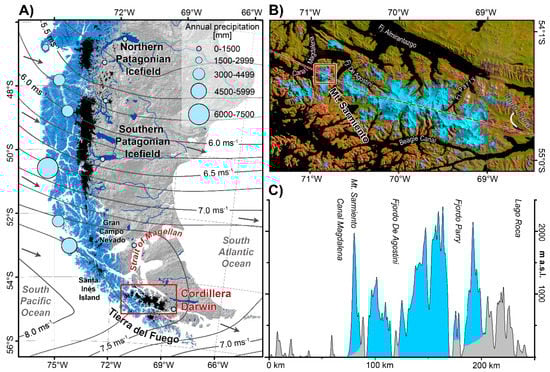
Figure 1.
(A) Overview of the Patagonian Andes and the Tierra del Fuego with its main ice bodies (black) [8]. On the upwind side of the mountain ranges, blue shades display precipitation amounts exceeding 1000 mma−1 [18]. Light-blue-filled circles and their diameters represent the location and the corresponding annual precipitation of climate stations (data obtained from the Dirección Meteorológica de Chile (DMC) and the Servicio Nacional de Meteorología (SMN)). Grey isotachs represent the mean annual wind speed in m per second (ms−1), and grey arrows, the mean annual wind direction for the period between 1980 and 2018 at 1000 mbar pressure level [19]. (B) The fjord-rich west–east striking mountain range of the Cordillera Darwin includes the largest icefield of Tierra del Fuego (Landsat-TM image mosaic, bands 5-4-3, acquisition date: 14-02-2005). (C) According to the west–east elevation profile of the Cordillera Darwin (transect displayed as red line in B), Monte Sarmiento is the first prominent peak located on the windward, hyper-humid side of the mountain range; glacierized terrain is displayed in blue.
The Little Ice Age (LIA) was a period of global glacial expansion from the 13th century to a maximum between the 17th and 19th centuries, and it is well documented [20,21]. However, the LIA showed a high spatio-temporal variability in a global context [4,20,22], and glacial fluctuations, e.g., for the Southern Hemisphere, do not completely coincide with those from the Northern Hemisphere [23]. In fact, significant differences in spatio-temporal glacial advances have emerged even within the respective hemispheres [20]. As a consequence, the term of a “global phenomenon” is controversial [24]. A considerable variability of the timing of the LIA maximum on decadal and centennial scales has been recorded [11,25]. Hence, a strong need for accurate dating of glacial fluctuations is apparent [11,26,27,28]. Indeed, the glaciers in the Southern Andes reached their LIA maximum extent at various times across several centuries, culminating between the 17th and 19th centuries [11,29]. Although the number of paleoclimatic studies in Patagonia has increased in recent decades, 85% of the implemented studies are still located on the eastern side of the Andean main crest [30]. Late Holocene glacial fluctuations have scarcely been documented for the glaciers in the Magallanes region; thus, the different phases of the “Neoglaciations” in Southern America are still corroborated by an insufficient number of studies [11,20]. With the exception of the LIA period, almost no information is available on glacial fluctuations within the last 2000 years. The Common Era (CE) is frequently subdivided in paleoclimatic periods based on (historical) observations or reconstructions conversant from the Northern Hemisphere [31]. The LIA is commonly preceded by the Medieval Climate Anomaly (MCA), which is considered to be a warmer period of approximately 400 years in duration (800–1200 CE) [32]. The Dark Age Cold Period (DACP, 300–800 CE) chronologically prior marked a distinctly cooler period which superseded the Roman Warm Period (RWP, 0–300 CE) [32].
Schiaparelli Glacier, within the Monte Sarmiento Massif, is located in one of the most western parts of Isla Grande de Tierra del Fuego (Figure 1B,C). The glaciers of this pronounced mountain peak descend from over 2000 m asl to almost sea level. West to Mt. Sarmiento, the Magdalena Channel directly connects the Strait of Magellan with the Pacific Ocean. This area has attracted scientific interest since the famous Beagle Expedition accompanied by Robert FitzRoy and Charles Darwin in 1836 [33]. Lithographs from this expedition supposedly show the Schiaparelli Glacier calving into the Magdalena Channel, leading to a dispute over the glacier’s extent in the 19th century [34,35,36]. To clarify whether the glacier calved into the sea within recent centuries, Masiokas et al. concluded that “[…] a more detailed analysis of this site, including the tree-ring dating of trees growing on the frontal moraines is needed to resolve this question” [11] (p. 257). The formation of moraines can be dated by the germination date of trees colonizing recently exposed glacial deposits [37]. In this study, we performed a tree-ring-based moraine dating of the terminal moraines at Schiaparelli Glacier: maximum tree ages constitute minimum ages for LIA maxima. Since an ecological proxy was used for dating, it is susceptible to uncertainties, e.g., a variable period between glacial recession and floral recolonizations (ecesis time) [38] or uncertainties due to missing the pith of the respective trees (pith offset) [39]. Commonly, dating uncertainty arising from the use of tree-rings on moraines is a quarter of a century or even more [26,40]. To compare phases of culminated glacial activity, the respective influences of the different uncertainty values on the dating accuracy must be disentangled. Consequently, one focus within the study was to provide a robust estimation of the uncertainties that emerge in tree-ring-based dating of glacial deposits. With these results, the plausibility of a fjord-calving glacier in 1836, as is inferred from the historical record, was verified. Furthermore, the study tried to constrain the timing and phases of different Neoglacial advances in Tierra del Fuego. Sub-recent trunks that were incorporated within morainic sediments were radiocarbon dated to interlink local glacial activities with the culminating glacial advances of southernmost South America during the Late Holocene.
2. Materials and Methods
2.1. Study Site and Regional Climate Conditions
In 2016, the 11 km long northwest facing Schiaparelli Glacier covered an area of 24.3 ± 0.3 km2 [8] and descended from 2207 m asl (Mt Sarmiento) to 11 m asl. The glacier calves into the moraine-dammed proglacial lake Lago Azul (~1.2 km2). The lake was formed after the glacier receded in the 1940s from its position located close to the terminal moraine system (Figure 2A). Satellite imagery and historical observation reveal that the Schiaparelli Glacier has been subject to a perceptible retreat within the recent decades. This clearly coincides with the widely observed behavior of land- and lake-terminating glaciers in the Cordillera Darwin [8]. While attempting to ascend the summit of Mt. Sarmiento in 1913, De Agostini [41] identified the glacier close to the terminal moraines behind a dense forest. During the following decades, the glacial terminus remained in the vicinity of the moraine system [35,36,42]. However, a continuous monitoring of glacial dynamics has only become possible since 1973, when Landsat MSS scenes first became available. As deduced from a TanDEM-X digital elevation model (DEM, acquisition date 13-05-2011, Microwaves and Radar Institute, German Aerospace Center (DLR), Oberpfaffenhofen), the terminal moraine system is composed of at least three major moraine ridges, reaching a maximal height of 35 m. The outermost moraine is located 2.2 km in front of the current glacial terminus. The moraine ridges are cut centrally by an approximately 60 m wide lake discharge, connecting Lago Azul with the Magdalena Channel to the west (Figure 2A,B).
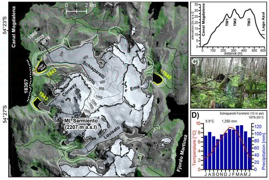
Figure 2.
(A) Overview of the study site at Mt. Sarmiento, including glacial margins [8,42] and their corresponding moraine ridges (light grey) and forest cover (green [43]). (B) Cross-section of the terminal moraine system as indicated by the red bar in (A). Three major terminal moraine ridges were identified (TM1–TM3). (C) Peat bog formation between the moraine ridges, colonized with Nothofagus betuloides trees of comparable diameter. (D) Climate diagram calculated as a mean of four CHELSA grids cells covering the end moraine [18].
The glacial forefield, especially the depressions between the moraine ridges, was characterized by abundant swampy terrain interspersed with several peat bogs. The hummocky terrain was colonized by a closed tree stand of Nothofagus spp., homogenous in height and diameter, indicating a simultaneous germination, i.e., subsequent to glacial retreat (Figure 2C). Recently, several tall individual trees had been uprooted by the wind, but no noticeably old and rotten trees were encountered on the ground. This implies that the forest is still at the stage of primary succession. Beyond the morphologically distinguishable moraine system, the forest stand was much more heterogeneous in terms of trunk diameter, species composition, and dead, decayed trees (climax forest).
Schiaparelli Glacier is surrounded by west–east striking lateral moraines at the northern and southern slopes, which reach elevations of 380 meters above sea level (m asl). In the upper hillside of the moraines, the forest stand appeared older and homogenous in its age structure, composed of N. betuloides and N. antarctica. Downslope of the lateral moraines towards the recent glacial margin, the tree stand was more scattered and small in growth, indicating a primary succession after glacial thinning. Above the lateral moraines, the matured forest was replaced by Andean tundra, composed of mosses, gramineous, lichens, and some low shrubs. The overall high annual wind velocities in Tierra del Fuego (Figure 1A) can intermittently exceed 30 ms−1 on exposed slopes, which can be decisive in forest distribution [44]. In sun-exposed and occasional wind-protected areas, the treeline can reach an elevation up to 550 m asl [15,45].
The late successional, undisturbed forest stand was mainly composed of the endemic evergreen southern beech (Nothofagus betuloides), with scattered individuals of Drymis winteri, Tepualia stipularis, and Nothofagus antarctica [46]. Since Nothofagus spp. saplings are shade intolerant, but can cope well with difficult nutrient recovery or soils containing low nutrient concentrations, they represent the pioneer woody species on recently exposed moraines after deglaciation. In addition, N. betuloides and N. antarctica grow superiorly on waterlogged soils; thus, they frequently occur in the glacial forefield [47,48,49]. Tree germination of Nothofagus spp. is epigeous and occurs in the spring of the year the seeds are produced [16,45]. The species composition represents the ecoclimatic hyper-humid zone of the sub-antarctic broadleaf evergreen rainforest, exceeding precipitation sums of 1000 mma−1 [47,50]. The dominance of N. betuloides is associated not only with a humid oceanic climate, but also with a cold-temperate climate [45].
The permanent cold air emanating from the ice-covered Antarctic continent, combined with the upwelling of cool Antarctic deep water, prevents substantial warming of the polar air south of 50° S and causes overall cool temperatures [51,52]. The daily and seasonal cycle is dampened by the immediate proximity of the ocean and the persistent westerlies. Since there are no climate stations in the vicinity that provide long-term data for a sound climatological classification (Figure 1A), we had to refer to the CHELSA reanalysis dataset (Climatologies at High Resolution for the Earth’s Land Surface Areas), downscaled from ERA-Interim to 30 arc sec [18] (Figure 2D). Temperatures were relatively homogenous throughout the year (mean temperature 5.9 °C), with an annual amplitude of merely 6.6 °C, and maximum and minimum temperatures during Jan/Feb and Jun/Jul of 9.2/9.0 °C and 2.7/2.6 °C, respectively. Interannual variations can be mostly attributed to the leading modes of atmospheric circulations: the Antarctic Oscillation (AAO), also known as the Southern Annular Mode (SAM) [53,54]. The SAM is defined by pressure anomalies of opposite signs over Antarctica and mid-altitudes, influencing the strength and latitudinal position of the westerly wind belt. During positive SAM phases, the southern westerly wind belt strengthens and shifts poleward and vice versa [55,56].
2.2. Methods for Dating Glacial Deposits (Based on Tree- Rings and Radicarbon Dates)
As soon as a formerly glacierized terrain becomes exposed due to glacial recession, tree seedlings colonize the bare ground, progressively tapering towards the glacial front [57,58]. The oldest individual trees found on a moraine can be used as a minimum estimation to date the formation of a moraine [38]. Nevertheless, the exact dating of the glacial event is influenced by some uncertainties that must be taken into account [39,59,60]:
- (i)
- the pith of the tree was not reached or missed during sampling (pith offset);
- (ii)
- the number of tree-rings that are lost when the tree is sampled at a distinct elevation above the ground;
- (iii)
- the timespan (ecesis time) between deglaciation (surface exposure), moraine stabilization, soil development, and the colonization by the first trees; and
- (iv)
- the probability that the oldest tree was sampled.
2.2.1. Establishment of Tree Ring Site Chronology and Evaluation of Missing Rings
Tree-ring width was measured with a precision of 0.01 mm after preparing the increment cores with a razor blade and chalk for better visibility of light rings. Since the vegetation period, and thus tree growth, extends over the turn of the year, the Schulman convention [61] is used for the Southern Hemisphere, whereby the year in which tree growth starts is used for dating. As recommended by Koch [39], all sampled cores were cross-dated statistically, and the established site chronology was verified against data from the International Tree-Ring Data Bank (ITRDB) using the open source statistical language R [62] and the dplR package [63,64].
If the increment borer missed the pith of the tree, the number of absent rigs must be estimated. The most widely applied geometric model, developed by Duncan [65], uses the curvature and width of the innermost visible ring to estimate the length of the absent radius. The number of missing rings is then calculated by dividing the estimated length of the missing radius with the mean width of the innermost 5, 10, and 15 visible tree rings [60,66]. If multiple radii are available, they are averaged to derive the mean ring width of the respective trees, and to additionally check for differences in eccentric tree growth [67]. The obtained correction factor is then added to the date of the innermost tree-ring to receive the age at coring height. As a prerequisite for this geometrically-based assumption, radial and symmetrical tree growth is required to estimate the length of the missing radius, leading to higher uncertainties with increasing numbers of missing rings [60,68]. So far, age uncertainties induced by the missed pith have only been estimated in a few studies, and must not be generalized across species or continents [60,67]. The effect of the intervals (first 5, 10, and 15 years) for calculating the mean ring width and the inferred pith offset (PO) was evaluated for 24 pairs of increment cores, one of which hit the pith of the respective tree, and another that missed it at a comparable tree height.
2.2.2. Growth Rate Modeling of Nothofagus spp.
Trees cored at a distinct elevation above the root collar do not reflect the date of germination and always underestimate the true tree age [69,70]. Since the root collar is located at or even below the ground level, an exact estimation of the tree age is highly time-consuming and destructive to the individual trees [70]. The study site was located in the Alberto de Agostini National Park as the core zone of the Cape Horn Biosphere Reserve, where it is prohibited to perform destructive sampling, such as taking cross sections at the root crown. Thus, we established a site-specific age–height relationship for Nothofagus spp. by sampling six young trees at different elevations above the ground level and counting the age differences between the distant cores of the respective trees. The dense and already matured forest of the terminal moraine was not suitable for this purpose, because a closed canopy influences the growth rates of young saplings [71,72]. In order to ensure comparable successional growing conditions, we selected the southern lateral moraine, which had been recently exposed after glacial recession, encompassing minimal soil development and scattered individual trees. Growth rates may vary considerably, as the tree stand may include highly stressed individual trees. In such cases, age estimations are prone to underestimating true tree age by more than 35 years [73]. For this reason, we carefully examined the increment cores extracted from the terminal moraine system to identify outliers in radial growth (more than 1.5 standard deviations calculated for the first 15 years in tree growth). To those outliers, an additional age-uncertainty of ±5 years was added, and it was ensured that they were not solely used for the dating of a respective moraine.
2.2.3. Estimation of the Site-Specific Ecesis Time
The ecesis time is spatio-temporally variable and does not follow a superficial dominant factor: it is rather the result of the combination of large-scale and local climatic influences, sufficient seeding availability, e.g., distance of seeding trees, seed dispersal, and the characteristics of the bedding substrate [38,57,74]. Previous estimations of the ecesis time in the Patagonian Andes and Tierra del Fuego have revealed a high temporal variability, ranging from less than one decade [75], to several decades [15], to even a century [34,76]. Even for the same glacier, adjacent slopes are colonized at rates differing by up to 30 years, depending on aspect and inclination [40]. The divergence of the tree colonization prevents a generalized application, and subsequently requires a site-specific determination of the ecesis interval [39,73]. Since a proglacial lake was located between the terminal moraine system and the recent glacial front, it was not possible to assess the ecesis time directly in the glacial forefield. Thus, the only possibility by which to examine tree recolonization after deglaciation was in the areas along the lateral moraines.
To evaluate which of the two lateral moraines was more similar in climatic conditions to the terminal moraine, we calculated the annual incoming solar radiation for the western side of the Sarmiento Massif. The calculation was based on a geometric solar radiation model using a digital elevation model as input, as implemented in the Solar Analyst tool in ArcView GIS (ESRI), developed by Fu and Rich [77,78]. The northern terminal moraine received only one third of the incident solar radiation due to cast shadows and steep slopes, whereas the southern lateral moraine was exposed to similar solar input as the terminal moraine system. Consequently, the ecesis time was estimated on the basis of samples from the southern lateral flank of the glacier.
On the southern lateral moraine at ~200 m asl, a significant change in the tree stand from a more or less dense/matured forest to a scattered tree stand was observed. That ecotone indicated a moraine stage that was exposed recently. Assuming a constant and linear glacial retreat, trees should be progressively more juvenile towards the glacial tongue. The individual trees that appeared the oldest along the moraine were sampled in transects between the recent glacial margin and the dense forest stand (Figure 3). Along this small lateral moraine, 81 young Nothofagus spp. were sampled at approximately 0.3 m above ground level. At least two cores were taken from each tree using an increment borer, and used for establishing a site chronology. The positions of the sampled trees were mapped using GPS with an accuracy of ±3 m and transferred to a geographical information system. Thereby, the spatial distance between the glacial outlines and sampled trees was precisely determined. Glacial retreat and tree succession was monitored by combining optical satellite imagery and tree-ring sampling for the last 40 years. To ensure that the succession was not disturbed by glacial advances, as they were observed elsewhere in the Cordillera Darwin [8,9], we performed multi-temporal observations of the glacial margins.
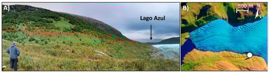
Figure 3.
(A) View onto the southern lateral moraine of Schiaparelli Glacier: red dotted line indicates the abrupt vegetation transition into a more dispersed tree stand. The sampling area was situated between the recent glacial tongue and the red lines. (B) Position and perspective of the photograph (A) indicated by white circle (background: false color composite Sentinel-2, acquisition date 04-07-2017).
For mapping glaciers and their variations, multi-spectral satellite imagery of sufficient quality has been available since 1973. However, reliable and sufficient imagery for southernmost South America is rare due to irregular satellite overflights and frequent heavy cloud cover. Therefore, 18 optical satellite scenes acquired from different sensors were used to assess regional glacial extent and variability (Appendix A Table A1). Scenes of the Landsat mission (MSS/TM/ETM+ and OLI) and Terra ASTER, acquired from the United States Geological Survey (Level 1GS/TP), were used for a semi-automated mapping of the glacier’s extent [8]. Additionally, satellite scenes from the Sentinel-2 MSI program of the European Space Agency (ESA) that has provided data since 2015 were used. All scenes were projected to the local UTM zone (19S) and checked for the orthorectification quality. Ratio images were calculated by dividing the raw digital numbers of the red and shortwave infrared channels [8,79]. We used the equivalent bands 2 and 4 for calculation of the ratio images in the case of the Terra ASTER satellite imagery. Due to the different resolutions of the respective ASTER bands of 15 m and 30 m, Band 4 was resampled to a 15 m resolution, as suggested by Kääb et al. [80]. A suitable threshold value was used after a stepwise increase of 0.1, starting from 1.0, to convert the ratio images into a binary image. By vectorizing the binary image, glacier polygons were generated and compared to false color composites of the mid-infrared, near infrared, and red channels. Afterwards, the glacial outlines at Mt. Sarmiento were subdivided into individual catchments using a void-filled UTM-projected DEM with a resolution of 30 m (SRTM, LP DACC NASA Version 3). The mapping accuracy was influenced by (i) the geolocation and (ii) the scene quality [81,82]. The positional error (i) was reduced by aligning the scenes used to distinct landforms like shorelines and prominent mountain peaks. The Sentinel-2 and most Landsat TM/ETM+ and OLI data matched perfectly, whereas the Terra ASTER and Landsat MSS appeared to have a small offset and were adjusted. Since scene quality (ii) is negatively influenced by seasonal snow cover, satellite scenes between the spring and autumn season, representing the seasonal snow minimum, were mainly used. In the case of partial cloud cover and occultation of the glacier, the next available and suitable satellite scene was used to supplement the cloud-covered parts of the original image.
The change and resulting uncertainty (u) in the position of the glacial margin by comparing two different satellite scenes was dependent on the respective image resolutions (r1 and r2) and the co-registration error (RE) due to the georectification process [83,84].
With a pixel size of 60 m, the Landsat MSS sensor had the lowest spatial resolution compared to the Landsat TM/ETM+/OLI (30 m) or the Terra ASTER and Sentinel-2 scenes (15 and 10 m, respectively). The largest possible uncertainty occurred between Landsat MSS (1973) and Landsat TM (1986) and accounts for 77 m, of which 10 m resulted from the RE. Hence, this uncertainty estimation is the worst-case value; we additionally estimated the precision of our semi-automated derived outlines by applying a positive and negative buffer to the glacial perimeter [85]. The buffer was applied to the glacial outlines before they were subdivided into individual catchments to prevent any uncertainty estimation where glaciers adjoined [81]. A buffer size of ±0.5 pixel of the sensor used (according to ±30, ±15, ±7.5, ±5 m) was well suited for the uncertainty estimation of clean-ice bodies [8,86,87], leading to a smaller maximum uncertainty than assuming that the complete pixel might be faulty.
2.2.4. First-Generation Trees
On older moraines, a very pronounced, old-grown dense forest can have evolved. In such areas, the identification of the oldest tree is not obvious due to its diameter, height, or branch spacing. Through a high number of sampled individual trees (>150 trees) we optimized the likelihood of identifying the oldest tree(s) growing on the moraine ridges [60]. The moraines were colonized by an uniform, dense forest stand which was comparable in diameter and height, with only a few dead trees and an abundance of the Nothofagus spp., typical for postglacial succession and first-germination trees [88]. Trees growing on the distal face of a glacial deposit can be much older than the ones on the proximal side of the moraine, because the latter can only germinate if the glacier completely retreated without any re-advances. Furthermore, the germination can be negatively influenced by katabatic winds [59]. If the glacier is still in the vicinity of the moraines, dumping and sliding processes of debris and meltwater may induce disturbances that additionally impair the natural recolonization. In order to avoid misinterpretations of the glacial position, trees were sampled at the respective moraine crest and at both the distal and proximal moraine faces.
2.2.5. Radiocarbon Ages
Radiocarbon ages (14C BP) received from the logs incorporated into the glacial deposits were calibrated using the CALIB 7.1 software [89] and the SHCal13 calibration curve for the Southern Hemisphere [90]. The median probability of the distribution function was used to report the calibrated radiocarbon age, whereby the calibrated date range is given as 2σ-ranges [91]. If the calibration provided multiple non-overlapping age segments, the period with the highest probability was used. The date notations of the radiocarbon dates are expressed as calibrated years before or after the Common Era (cal BCE/CE) or as calendar years before present (cal ka BP: ka = 103 cal. years BP, present = CE 1950).
Since different proxies such as tree-rings or radiocarbon data typically use different date notations, we have reported all dates within the manuscript in a uniform convention, using the Common Era as reference system. The calibrated radiocarbon ages are always denoted with the prefix “cal,” and are rounded to the nearest ten years and are expressed as highest probability for better readability. The original, exact calibrated and uncalibrated dates are listed in Table A2 and Table A3.
3. Results
3.1. Dating Uncertainty Introduced by the Estimation of the Pith Offset (PO)
Initially, the influence of the different intervals used to calculate the average ring width of the innermost rings was analyzed. The mean ring width varied insignificantly for the first 5, 10, and 15 years, leading to a maximum deviation that did not exceed 0.8 years if the PO was calculated afterwards. This was mainly attributed to the uniform growing conditions of Nothofagus spp. within the first years and the absence of strong inter- and intraspecies competition, e.g., for light, as the early successional forest does not provide a closed canopy.
The estimated PO and true PO were significantly (r = 0.64, p < 0.01) correlated, as the simple linear regression model revealed (Figure 4A), but showed higher variance with increasing distance to the pith. This was confirmed by the comparison of the estimated PO with the resultant PO errors (POerror = POestimated − POtrue) in the lower panel of Figure 4A: if the estimated PO was less than 10 years, the PO error resided between −8 and +5 years. This led to an over- or underestimation of the true PO by an average of 2.8 years (σ = 2.0). Due to the low number of observations, we calculated the expanded uncertainty by multiplying the combined standard uncertainty with an appropriate coverage factor (for 0.99 confidence), leading to an average PO deviation of 2.8 ± 1.4 years. For the trees with an estimated PO of less than 10 years, we consequently applied an uncertainty value of ±4 years.
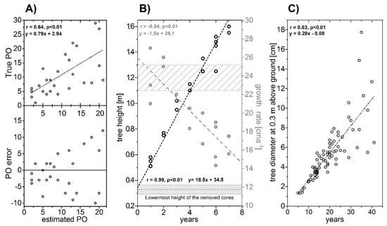
Figure 4.
(A) Scatter plot of the estimated pith offset (PO) in relation to the true PO (upper panel) and the PO error (lower panel). (B) Tree height in dependence of the counted tree-rings and resulting growth rate. The grey shaded area displays the lowermost coring elevation on the lateral moraine, the grey hatched area indicates coring height on the terminal moraine system. (C) Graph comparing increasing trunk diameter respective to tree age for trees sampled on the lateral moraine.
Verifiably, the number of incorrectly estimated annual tree-rings increased with growing PO, reaching maximum values of −10 and +12 years, respectively. In accordance with the above procedure, the average PO uncertainty at 0.99 confidence limit accounted to 7.3 ± 2.0 years, leading to an uncertainty value of ±9 years for trees with an PO exceeding 10 years. According to Hochreuther et al. [68], we restricted the reliable PO estimation and disregarded trees with more than 20 calculated missing rings to prevent an over- or underestimation of the true tree age.
3.2. Growth Rates of Nothofagus Spp.
The Nothofagus spp. pioneer species located at the lateral moraine were sampled between 0.30 and 0.40 m above their root collars, with an average sampling height of 0.33 m above ground level (Figure 4B). The age of the lowermost extracted cores was used as the starting reference, but did not represent the true tree age. Subsequently, the temporal difference to the next distant core, which was sampled further up the trunk of the respective tree, was calculated. The cumulative temporal differences (i.e., the effective ageing) depending on the respective height are displayed in Figure 4B. Variations in tree height accumulate as the trees mature, resulting to only minor variations at a young age (less than 0.1 m for the first year of growth) and larger variations (0.3 m) for trees aged over six years. This indicates higher age uncertainties with increasing sampling height above ground level. Finally, annual growth rates were expressed by calculating the differences in height and counted years of the extracted cores (Figure 4B).
Growth rates are highest as a sapling, reaching values exceeding 25 centimeters per year [cma−1]. With increasing maturity, growth rates show a declining trend (r = −0.84, p < 0.01) and reach minimum values of 14 cma−1. The average growth rate amounts to 20 cma−1, whereas saplings smaller than 1.2 m show an enhanced annual growth rate of 23 cma−1, and trees larger than 1.2 m, a distinctly reduced growth rate, corresponding to 18 cma−1. From a physiological perspective, the sampled trees did not show any growth anomalies such as narrow rings. Additionally, the development of multiple branches at the base of the trunk or compression wood, which would indicate straining and detrimental growth conditions, was not visually apparent. The increase of the tree diameter (~0.3 m above ground level) for the 81 collected trees was quite constant (r = 0.83, p < 0.01) and showed only minor deviations within the first 15 years, but increased with aging of the tree (Figure 4C). The apparently steady and undisturbed growth patterns at young age on the lateral moraine justify a generalization of the calculated growth rates to the entire set of sampled trees.
Considering the average growth rates for the first three years (24 cma−1), the trees that were sampled at the lateral moraine about 0.3 m above the ground must have been at least two years old. Sampling height at the terminal moraine of 1.2 m might vary slightly ±0.1 m (indicated as hatched field in Figure 4B) due the rugged and hummocky terrain or interfering branches. As depicted in Figure 4B, the two year old trees sampled at the lateral moraine reached a coring height of 1.2 m within a further 5 ± 1 years. In consequence, the trees sampled on the terminal moraines would reach, under comparable growing conditions, their coring height within 7 ± 1 years.
3.3. Site-Specific Ecesis Time
The average glacial retreat on the southern lateral moraine was calculated as the mean of the orthogonal distance every 30 m to the respective glacial margins. From 1973, Schiaparelli Glacier receded continuously in the lateral direction by 215 m (r = −0.99, p < 0.01) until 2018, which corresponds to an annual loss of approximately 5 ma−1 (Figure 5A,B). The high error values given in Figure 5 (light grey) describe the largest possible error, caused by the assumption that each of the individual examined pixel pairs of two satellite scenes to be compared is faulty [83], which is, concerning the location of the seedlings, rather unlikely. If, on the other hand, the uncertainty between two satellite scenes were calculated using the applied buffer, which assumes that the accuracy of the glacial boundaries is ±0.5 pixel of the used sensor, the calculated error for the lateral glacial retreat is significantly lower (dark grey).
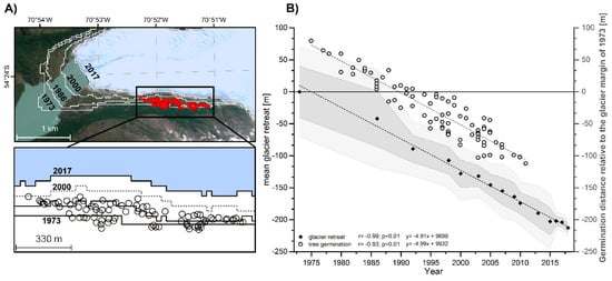
Figure 5.
(A) Geolocation of the sampled trees at the southern lateral moraine in relation to the glacier’s margins between 1973 and 2018 (background Sentinel-2, 03-08-2017). (B) Mean glacial retreat along the lateral moraine, including tree germination as a dependency of the glacial margin in 1973. Trees with positive and negative distance values germinated outside and inside the 1973 glacial extent, respectively. Light grey and grey areas indicate the maximum possible uncertainty by comparing two glacial outlines (i.e., ±1 and ±0.5 pixel of each satellite pair to be faulty).
The germination date as dependent on the distance to the glacial margin in 1973 is displayed on the right ordinate axis in Figure 5B. Trees with a positive distance germinated outside the 1973 glacial extent. All trees with negative values germinated on freshly exposed terrain subsequent to glacial recession. The succession of Nothofagus spp. along the 1.3 km long sample site was rather swift and extensive. The trees that appeared the oldest were sampled, and the simple linear regression analysis (r = −0.93, p < 0.01) revealed that the saplings linearly traced the glacier’s retreat (r = −0.99, p < 0.01) (Figure 5B).
According to the two linear models, the germination of the trees took place parallel to the glacial retreat with a time offset of 15 years. Although the colonization of some individual trees on deglaciated deposits can occur very fast (<10 years), the assumption of such a short period for a generalized ecesis period is hardly reasonable. On the one hand, the number of successional trees that germinated shortly after the retreat was relatively small, with the possibility of sampling them later in a dense forest as well. On the other hand, the estimates of the ecesis time recorded on the lateral moraine weretransferred to the frontal moraine system. Due to sliding and dumping processes, the morphological moraine patterns of the lateral moraines were less dissected than those of terminal moraines [92]. Glacial oscillations can lead to complex pushing, thrusting, and dumping processes at the glacial terminus, combined with melt-induced collapses that may result in steadily disturbed moraine formations [93,94]. It is likely that tree colonization will be delayed in such unsettled terrain compared to the relative flat or undisturbed lateral moraine. Therefore, the shortest possible time interval derived from the few first germinated individual trees was not used, but an averaged time delay of 15 years, as revealed by the regression analysis, was used instead. An associated uncertainty value of ±3 years, derived by the standard deviation of the linear model, was applied, resulting in an ecesis interval of 15 ± 3 years.
3.4. Tree-Ring-Based Moraine Dates
The root-mean-square error (rmse) for the tree-ring dating of the terminal moraine can be described as the quadratic sum of the independent uncertainty of the PO estimation (±4 or ±9 years), the growth rate model (±1 years), and the ecesis time (±3 years), leading to a minimum and maximum uncertainty of ±5 or ±10 years.
The forest distribution was strongly linked to the presence of glacial deposits which seemed to favor the formation or quality of soils, as the closed forest was exclusively located on glacial debris. At altitudes above 100 m asl, the appearance of trees was solely attributed to the presence of moraines, which simultaneously represented the local tree line (Figure 6A). The digital elevation model of the TanDEM-X scene indicated at least three terminal moraine ridges north and south of the lake discharge. The field survey revealed an irregular distribution of the forest within the terminal moraines: a vast area north of the lake runoff in which numerous ponds appeared, with trees growing in a scattered pattern. According to the historical information, this area was still glacierized, or had just been recently deglaciated, in the 1940s [36,41] (Figure 2A), which was reflected by the occasional vegetation typical of the successional stage, as was also observed after the subsequent glacial retreat of 1973 (Figure 6A). This was supported by the comparison of Sentinel-2 scenes acquired from different seasons, which revealed that the generally dominant evergreen N. betuloides was, to a significant extent, substituted by the broadleaf deciduous N. antarctica (Figure 6A). The latter species is habitually adapted to higher elevations (>100 m asl) but is also abundant in flat and wet terrain, e.g., directly along lakeshores, wetlands, and on recently exposed terrain [16].
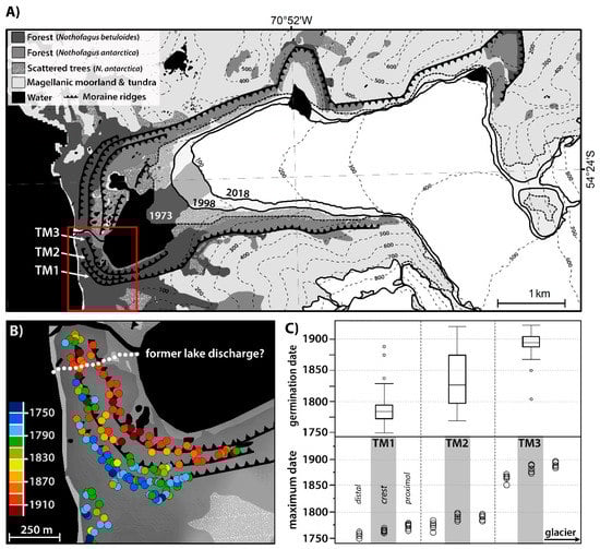
Figure 6.
(A) Landforms and vegetation distribution in the glacial forefield of Schiaparelli Glacier. (B) Germination dates of the individual trees sampled on the terminal moraine system. Different colors display germination periods. (C) Overall age structures of the TM1–TM3 moraine systems (upper panel) and germination dates of the five oldest trees with respect to the geolocation on the moraine slopes (lower panel).
The presence of multiple ponds, the simultaneous onset of peat bog formation, and the scattered appearance of N. Antarctica, which often comprises several trunks or forms belts of krummholz [95], appeared unfavorable for tree-ring-based dating of the glacial deposits. In consequence, our moraine dating was concentrated on the area south of the outflow (Figure 6B), as the forest in the area appeared to be older and the terrain was less unsettled.
Additionally, the shape of Lago Azul reflects the glacier’s principal ice flow direction and is aligned on its elongated axis exactly towards the dated terminal moraine system, supporting the hypothesis that these moraines are representative of former glacial activity.
Along the three terminal moraine ridges (TM1–TM3), the maximum tree age increased with increasing distance to the glacier, whereby the outermost terminal moraine encompassed the oldest trees and the innermost, the youngest ones. This implies a glacial recession without distinct readvances that would superimpose the TM1 moraine since its deposition date. The oldest sampled tree individual, germinated in 1749 CE, was located on the distal side of the TM1 moraine crest in the southeastern part, representing the maximum date of moraine stabilization (Figure 6B,C). Two additional trees nearby on the proximal slope of the moraine germinated in 1763 CE and 1764 CE, representing the minimum deposition date of glacial sediments. However, the mean germination date of the five oldest individual trees from the proximal moraine slope was about 10 years younger than those from the distal slope (Figure 6C, lower panel). This suggests that the terrain was either still ice-covered for a longer period, or that the glacial front was located nearby. Glacial oscillations, as well as unfavorable site-specific climatic circumstances (e.g., katabatic winds), meltwater streams, or collapse structures introduced by dead ice may impede otherwise rapid colonization. The clearly discernible TM1 moraine ridge diminished in contour in a northwesterly direction and transformed into a diffuse hummocky terrain with multiple small ridges, with the oldest trees in that area dated to 1769 CE.
Tree recruitment on the central moraine TM2 seemed to be most heterogeneous, with the largest age range of germination dates between 1762 CE and 1921 CE (Figure 6B,C). Similar to the TM1 moraine, trees along the moraine belt towards the lake discharge (in northern direction) were slightly younger. South of the recent lake drainage, the TM2 moraine belt was interrupted by an abrupt terrain flattening and the occurrence of swampy terrain. Simultaneously, tree age was youngest in this area (average germination date 1895 CE), and the individuals appeared stunted and possessed multiple trunks, indicating harsh growing conditions. Some individuals showed clear signs of root exposure, e.g., due to fluvial geomorphic processes, such as the presence of a former lake outflow (Figure 6B). The oldest trees on the distal slope in the southeastern part of the TM2 moraine dated back to 1760 CE, while the oldest trees towards the north were 20 to 30 years younger, corresponding to 1782 CE and 1786 CE. Tree germination on the distal slope of TM2 coincided with the proximal TM1 moraine side around 1760–1775 CE, whereas tree recruitment on the TM2 crest and proximal side had a relative lag of approximately 15 years (Figure 6C).
This observation was decisive, since the TM2 moraine belt was almost radially dated before the 19th century, and a calving of the glacier into the Magdalena Channel, as outlined by the Beagle Expedition’s lithograph in 1836 CE [33], seems rather unlikely.
Tree recruitment on the terminal moraine closest to the glacier (TM3) was dated to 1850 CE and possessed the smallest age range. Only one older tree was dateable at the easternmost site (1807 CE). The tree position was situated in a transition zone, where the narrow, barely distinguishable lateral moraines fanned out into defined terminal moraines. This individual tree distal to the TM1 moraine was therefore attributed to the proximal slope of the TM2. Around 1900 CE, the glacier receded so far that the proximal TM3 side was recolonized with trees.
3.5. Radiocarbon Dates/Glacier Chronology of Southern America
In total, 14 trunks (Table 1) incorporated within the terminal moraine deposits of the Schiaparelli Glacier were discovered, of which five were located directly on the lakeshore south of the lake discharge. The remaining trunks were exposed along the moraine cross section parallel to the river bed. The disordered location of the trunks amidst glacial debris suggested that the trees were killed and deposited during glacial advances. Samples for radiocarbon dating were taken from the trunk exterior to determine the glacial event more precisely.

Table 1.
Radiocarbon ages of trunks found within the glacial forefield. Most probable ages of the calibrated dates in parentheses, spanned by maximum and minimum ages of the 2σ range.
After tree mortality, sapwood is less resilient to environmental influences than heartwood, which may cause dating uncertainties. However, we observed one trunk still showing morphological signs of an intact sapwood area, leading to the conclusion that the trees were covered rapidly after they were overridden and tilted by the glacial advance. Consequently, we assumed that dating uncertainties were of subordinate importance.
With regard to the slope morphology and the low tree line, we considered it unlikely that the trees might be remnants of a forest that collapsed from the lateral slopes after glacial thinning, or was eroded by glacial advance and later transported and accumulated by the glacier. We hypothesize that the trees grew in the apron of the glacier near the terminal moraines, and were buried and transported by glacial advances more or less in situ. Statistically, multiple 14C dates were available for the same glacial/deposit event. The standard deviations of SC 1–5 could be clustered according to their time overlap and attributed to one single glacial event. The same applied to samples SC 6–9 and SC 10–11, whereas three single glacial oscillations (SC 12, SC 13, SC 14) at 880 CE, 1000 CE, and 1220 CE could be dated.
4. Discussion
4.1. Late Holocene Glacial Oscillations in Southernmost America
Even though temperatures in the Early Holocene were up to 2 °C higher than in the late 20th century [25], it is highly unlikely that the glaciers disappeared entirely at this time. High precipitation amounts cause a considerable accumulation rate on the hyper-humid side of the Andes. Even under the recent climatic conditions, elevation changes for the glaciers of Tierra del Fuego region have been balanced or even positive above 900m asl [96]. In consequence, the mass and area loss mainly affected the glacial tongues and low elevated glacial areas, leading to a severe glacial retreat. After this prolonged phase of glacial recession in the Early to Middle Holocene (8200–4000 BCE), many glaciers in the world were subject to a glacial resurgence that was initiated between the Middle and Late Holocene (~4200–2500 BCE) [14,97,98]. This period is referred as the “Neoglacial” [97,99,100], and the cooling within the Neoglacial lasted until ~1900 CE. The most recent phase of supra-regional intensified glacial advance is referred as the LIA with regard to glaciation (~1250 CE to ~1950 CE) [20,22]. Irrespective of the definition of the LIA, namely whether a glaciological or a climatological concept is used, the timing and duration is globally and interhemispherically highly variable [22,101].
For the Patagonian Andes the most common glacier chronologies were published in 1965 and 1995/2013 by Mercer and Aniya, respectively, postulating three to five phases of glacial advances, which are named in decreasing age as Neoglacial I–V (NG I–V) [12,102,103]. Nevertheless, lately, studies have provided important evidence for the occurrence of up to seven phases of culminated glacial expansions in the last 10,000 years [14,104,105]. Most of the data on which the glacial chronology of Southern America is based are represented by radiocarbon-dated glacial deposits. The inferred 14C ages are frequently based on single measurements, and it cannot be ruled out that organic material has been remobilized or overprinted by Late Holocene advances. Therefore, glacial events/chronologies in Southern America are not always well constrained in time [4,30,97], and should be best regarded as broad regional trends [25].
Glacial advances within the last 2500 years are compiled in Figure 7 for the Southern Patagonian Icefield, including adjacent mountain glaciers (~48–51° S) and the Magallanes–Tierra del Fuego region (~52–55° S). Several phases of culminated or enhanced glacial activities can be inferred (displayed as blue vertical bars in Figure 7A,B, Table A2) [4,11,16].
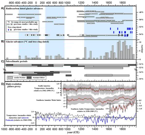
Figure 7.
(A) Glacial advances depending on the latitude, displayed as calibrated 14C 2-σ/1-σ uncertainty range (for detailed list of the used references refer to Appendix B Table A2) and tree-ring-based moraine dates from the Tierra del Fuego region [16,117]. Blue vertical bars indicate phases of enhanced glacial activity. (B) Frequency of glacial advances at 25 year intervals, including tree-ring-derived advances compiled in Masiokas et al. [11]. (C) Paleoclimate studies representing (un)favorable climatic conditions for glacial expansion (Table A2). (D) High resolution palaeoclimatic reconstruction for South America [118], Southern Annular Mode Index [119], Southern Andes Temperature Anomalies [120] (red lines represent the respective 11 year fast Fourier transform (FFT) filter for each time series), and Temperature Anomalies for the Antarctica [121].
The lower part of Figure 7 compiles paleoclimatic studies from southernmost South America that represent favorable or unfavorable climatic conditions for glacial growth. In fact, no simple interrelationship between glacial oscillations and climatic variables exists, but rather, a complex interweaving of climatic and non-climatic factors. Even glaciers that are in contact in the accumulation zones (located side by side) and are subject to the same local climatic influences can exhibit contrasting frontal variations due to different accumulation–area ratios (AAR) [106,107]. In addition, the calving rate of a respective glacier is decisive for its length variation. Calving fluxes represent inherent dynamic instabilities resulting, for instance, from a complex interaction between subsurface geometry, sub- and englacial water pressure, ambient water temperature, and circulation, tide, and waves [108,109,110], and are frequently decoupled from direct climatic influences [97]. Therefore, the evidence of glacial fluctuations and the imprints of climate signals must be critically assessed, especially in regions with tidewater- and lake-terminating glaciers [97,111].
The timing of the Neoglacial (NG) advance between ~550 BCE to 50 CE in southernmost South America is mostly based on the dating of glacial deposits from Upsala Glacier (~49°40′ S) and Occidental Glacier (~48°50′ S), descending from the eastern and western side of the SPI, respectively [12,34,102]. There has been so far no clear evidence by morainic deposits that the southern glaciers of the Magellanes–Tierra del Fuego region reacted in phase to that NG event. In contrast, at the Gran Campo Nevado Ice Cap, the lack of evidence for glacial advances between 3000 BCE and 1000 CE, raised the question of a possible shift of the westerlies and resultant drier conditions [112]. However, the new data derived from the Schiaparelli Glacier closes this gap in knowledge, indicating at least one glacial advance during that NG, with the oldest date estimated at 280 cal. BCE. The five radiocarbon dated samples SC 1–SC 5 (Table 1, Figure 7A) suggest several glacial advances before 110 cal. CE. This is corraborated by glacial clay deposition derived from a marine geological fjord core at Marinelli Fjord (54°25′ S), suggesting glacial advances between 350 cal. BCE and 150 cal. CE, and a subsequent retreat lasting until ~550 cal. CE (Figure 7C) [113].
The Neoglacial stage ~300–850 CE is reflected in our study by two advances: four individual trees (SC 6–SC 9, Table 1) and their 14C ages were indicative for a first advance around 300 cal. CE, followed by a second advance between 670–770 cal. CE (SC 10–SC 11). Although the first glacial advance is so far the only evidence of glacial activity at the beginning of this NG in Tierra del Fuego, the latter one coincides with the glacial advance at Ema Glacier (790 cal. CE) [15]. Ema Glacier descends from the eastern flank of Mt. Sarmiento (54°25′ S, Figure 2A). The synchronous advance of the two glaciers reveals a similar glacial behavior to a common climate forcing. The NG event is additionally reaffirmed by several studies in the area between 51° S to 54° S, representing a phase of stable/common climate forcing for the period from ~600 cal. CE to ~900 cal. CE, favorable for glacial advance (Figure 7C) [10,113,114].
In contrast, recent studies at the fjord of Marinelli Glacier (~54°33′ S), northern side of CD) have indicated a massive retreat, with its maximum roughly centered between the neoglacial events at ~300 CE [10,113,115]. At Almirantazgo Fjord, north of Marinelli Glacier (Table A2), a significant meltwater event was detected by the use of a grain-size model between 50 BCE and 750 cal. CE, indicating a rapid retreat of the respective glacier combined with a high meltwater discharge [10]. Vanneste et al. [115] found evidence in elevated glacial dust deposits that the Marinelli Glacier receded so far that it was no longer fjord-terminating, but land-terminating in ~250–350 cal. CE (Figure 7C, Table A2). These results are in disagreement with the dated glacial advance of Schiaparelli Glacier around 300 CE. Nevertheless, the Marinelli Glacier features some peculiarities, e.g., an exceptional high length reduction since its LIA position. The length reduction along the glacial centerline exceeded 14 km and was around seven times as high as that of Schiaparelli Glacier [8]. Concurrently, and in contrast to the surrounding glaciers, high flow velocity and extreme glacial thinning have been observed within recent decades at Marinelli Glacier [96,116]. It appears that non-climatic factors, e.g., bedrock topography, fjord bathymetry, and calving processes, are considerably influencing the glacier’s behavior [9,116]. In consequence, we assume that the glaciers descending from the northern part of the CD may respond differently, or even complementarily, than the glaciers of the hyper-humid western and southern mountain range [9]. This points to the fact that paleoclimatic evidence is not valid when generalized, and therefore must account for differences in terms of glacial exposition/location. This is in line with a review paper dealing with the paleoclimatology of southernmost South America, which highlighted the inconsistent/opposite picture that can be derived from the interpretation of various proxies [30].
Climate reconstructions for the period of the last two millennia have revealed a globally decreasing temperature trend [101,122]. This can be well observed on the Antarctic continent, where temperature reconstructions for the entire Antarctic show a negative trend until the 20th century (Figure 7D). This cooling has been reinforced by a progressive shift of the Southern Annular Mode towards positives phases since 1400 CE (Figure 7D), which also causes a warming of the Antarctic Peninsula [119].
Between the penultimate and last NG advances, glacial activity is noticeably declining. This is also reflected in the small number of dated glacial advances and climatically unfavorable conditions for glacial growth (Figure 7B,C). This phase coincides with the period of the Medieval Climate Anomaly in Southern Patagonia [4,114,120]. However, Schiaparelli Glacier still presents glacial activity at the onset of this climate anomaly (SC 13). The high-resolution data series are also rather ambivalent: the warmer period (1150–1350 CE), which can be discerned in the temperature reconstruction of South America (Figure 7D), reveals a temporal offset compared to the culminated glacial advances [118]. During this phase of moderate/higher temperatures, the reconstructed Southern Annular Mode (SAM) [119] has also exhibited less negative values. The core zone of the Southern Hemispheric Westerlies is located between 50 and 55° S. In a positive phase of the SAM, this windbelt contracts towards the pole and weakens the winds between 40 and 50° S, and vice versa [1,123]. After 1350 A.D., a significant decrease in the reconstructed temperature and also a prolonged period of exceptionally negative SAM indices can be considered to mark the (climatological) onset of the LIA. Negative phases of the SAM denote an increasing moisture transport with expanded/enhanced westerly winds north of 50° S, which nourish the large ice masses of the SPI and NPI, and are in consequence favorable for glacial growth.
The latest 14C-dated glacial event at the Schiaparelli Glacier occurred around 1225 cal. CE (SC 14), and corresponded to the start of the Little Ice Age. Most glacial advances in Southern Patagonia during the LIA are dated between 1200–1350 CE, 1560–1675 CE and between the 18th to 19th century [4,14,117,120] (Figure 7). In the Magallanes region at Pia Glacier (54°46′ S), two radiocarbon dates reflect neoglacial maxima of multiple moraine ridges formed between 1140–1340 cal. CE. The last date corresponds to a noticable advance of the Ema Glacier, leading to the conclusion that the glaciers south of the Strait of Magellanes advanced during the LIA in the early 13th to 14th century. Paleoclimatic records support this phase of accentuated glacial growth as a uniformly cool/moist phase (Figure 7C). A tree-ring-based climate reconstruction performed by Villalba et al. [124] in the southern Andes revealed that the LIA temperatures were about −1.5 °C less than today. Since 1800 CE, temperature have followed a positive trend that was only slightly interrupted at the beginning of the 20th century.
Tree-rings as a proxy for glacial activitiy have provided more accurate dating results in recent centuries compared to the radiocarbon method, which features calibration problems [125]. As Nothofagus spp. are long living species and the moraines are quickly recolonized, the tedious task of seeking sub-recent wood for 14C dating can be omitted. Therefore, the number of tree-ring-based dated glacial advances has increased since ~1600 CE, as also reflected in the absolute number of glacial advances compiled in Figure 7B. In the Tierra del Fuego region, recently exposed glacial deposits were dated using tree rings at only three locations: Gran Campo Nevado Ice Cap (Lengua Glacier), Santa Inés Island (Alejandro and Beatriz Glaciers), and Mt. Sarmiento Massif (Ema Glacier) (Figure 1A, Figure 7A) [15,16,117]. The oldest tree-ring-dated glacial advances were substantiated to 1628 CE and 1675 CE at Lenguna Glacier and Alejandro Glacier, respectively. All the subsequent glacial advances were smaller in their glacial demension and did not reach the extent of their precursor. Two reworked stumps embedded until 1577 and 1555 cal. CE represent an advance at Glacier Ema. In the forefield of the Schiaparelli Glacier, no evidence was found for an advance between 1400 CE and 1700 CE. However, the moraine formation ~1750–1850 CE for the glaciers of the Mt. Sarmineto Massif appears to have been synchronous. Additionally, the moraine formation coincides with tree-ring-dated moraines from Santa Inés Island [16] and the Gran Campo Nevado Ice Cap [117]. Centered around ~1750 CE, all studied glaciers of the Magellanes region south of 52° S revealed an advance (Figure 7A). Due to the southward shift of the Southern Westerlies during the positive phases of the SAM in recent decades [55], or as a prolonged period since the end of the LIA, there has been a slight increase in precipitation at the western side of the Cordillera Darwin of +200 mma−1, whereas precipitation in Northern Patagonia has been significantly declining (up to −800 mma−1) [1]. This could lead to glacial thickening in the accumulation area and compensate for possible warming tendencies in Tierra del Fuego, as observed at the Gran Campo Nevado Ice Cap [126].
Although the TM2 and TM3 moraines are situated close to each other at Schiaparelli Glacier, the moraine at the distal shore of the proglacial lake is about 100 years younger, leading to the conclusion that the glacier stagnated over a longer period in this position or that a readvance took place at the end of the 19th century (Figure 6C and Figure 7A). During a four-year British expedition with the ship “Alert” between 1878–82 CE, the Fuegian–Magellanes region was explored, discovering an advance at Glacier Bay (53°20′ S/72°50′ W) and describing it as “(…) a strange sight, standing in the middle of this terminal moraine, to see, on the one hand, a fresh evergreen forest abounding in the most delicate ferns and mosses; and, on the other, a huge mass of cold blue-veined ice, which was slowly and irresistibly gouging its passage downwards to the sea” [127] (p. 125). This glacial advance, destroying the forest after a period of prolonged glacial inactivity, supports the hypothesis of a late 19th century synchronous advance of the Magallanes glaciers.
In the first half of the 20th century, many glaciers located on the hyper-humid side of the CD were still close or at their Late Holocene maxima [9,15]. Whereas most of the fjord-terminating glaciers are calving in constant positions or have even revealed some readvances in recent decades, the lake-terminating glaciers are mostly retreating [8]. This is also valid for Schiaparelli Glacier and Ema Glacier, which were situated in the vicinity of the terminal moraines in the early 1940s [15,35,42]. Since then, these glaciers have been subject to a significant retreat. The glacial recessions along the glacier centerlines of Schiaparelli and Ema Glaciers are displayed in Figure 8A, revealing an almost continous retrat of 2000 m during the last ~75 years. The area of Schiaparelli Glacier decreased by 2.8 ± 0.7 km2 between 1973 and 2019 (Figure 8B). The area loss has been accompanied by a rapid thinning of the glacial tongue, exceeding values of −4 ma−1 since 2000 [96]. This indicates that Schiaparelli Glacier has been very sensitive to climatic changes in recent decades, and reacts more rapidly than the surrounding fjord-terminating glaciers.
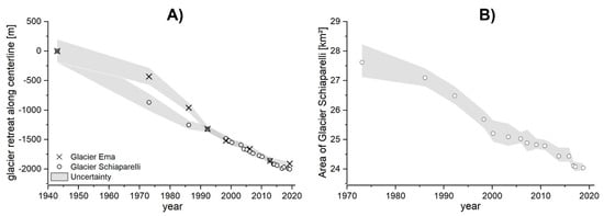
Figure 8.
(A) Glacial recession along the centerline of Ema Glacier and Schiaparelli Glacier, derived from satellite imagery (Table A1). Uncertainty values were calculated according to Equation (1). For historical information of 1943, an uncertainty value of ±100 m was assumed. (B) Area loss of the Schiaparelli Glacier. Uncertainty values were calculated applying a buffer of ±0.5 pixel of the sensor used.
4.2. Variables that Influence the Uncertainty Value for Tree-Ring-Based Moraine Dating
4.2.1. Estimations of the Pith Offset (PO)
Previous studies estimating the error range of PO have observed that for small distances (few missing rings), the true PO was overestimated, and in contrast it was underestimated for larger distances [60,128]. Our results support these observations to the extent that the deviations increased with increasing PO. Nevertheless, our study did not reveal a clear assignment of an over- or underestimation dependent on the distance. The uncertainty value for the PO of the Nothofagus spp. was in good agreement with a study recently performed in High Asia [60] indicating that an estimated PO of more than 20 years may underestimate the true tree age by more than 10 years. If moraine dating is based on tree-rings and glacial fluctuations are to be compared on a decadal scale, we highly recommend disregarding PO estimations that include more than 20 missing rings.
4.2.2. Height–Age Calibration
Our results revealed that high averaged annual growth values of almost 0.25 ma−1 for the young Nothofagus spp. encompassed only minor fluctuations. This is in line with growth rates observed within the hyper-humid zones of the evergreen Magellanic forest on recently exposed glacial deposits even exceeding values of 0.30 ma−1 at the southern part of the CD [117,129]. The single available study in Tierra del Fuego examining the growth rates for southern beech was performed at the small Gran Campo Nevado Ice Cap, and revealed similar but more variable growth rates [117]. However, the sampling site was located 100 m asl higher and received up to three times as much precipitation as our sampling site at Schiaparelli Glacier. This may lead to more unfavorable growing conditions, but highlights the resilience and wide ecological niche of Nothofagus spp. Constraining conditions seemed to be absent within the first years of tree growth, as indicated by a relatively homogenous increase of the tree radii. If tree growth is suppressed, miscalculation or underestimation of true tree age can exceed 35 years when cored at breast height [60,73]. High mountain areas possessing trees at the forest ecotone, crossing the treeline up to the krummholz limit, are particularly affected. Therefore, trees should be carefully checked for tree physiological evidence of aggravated growth conditions before they are incorporated in dating, and must be excluded when appropriate.
4.2.3. Ecesis Time
The ecesis time is the variable highly affecting the accuracy of tree-ring-based moraine dating. At the same time, it is also one of the most difficult parameters to determine, since it is usually estimated on the basis of historical sources and the maximum age of the pioneer trees, which are both susceptible to errors [26,103]. Frequently, the succession of pioneer trees on recently exposed geomorphological terrain, e.g., landslides and floodplains subsequent to lake outburst floods, is used as an evaluation of the ecesis time [26,66]. The germination of seedlings is strongly dependent on the bedding substrate, which does not necessarily have to be the same for, for example, floodplains and moraines, and can possibly lead to further estimation mistakes. This high variability in the ecesis period is compiled in Figure 9 for the southern Patagonian Andes.
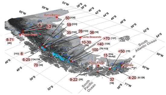
Figure 9.
Overview of different ecesis intervals for trees colonizing recently exposed glacial deposits in the Patagonian Andes. Numbers highlighted in red represent the intervals; numbers in square brackets represent the respective reference study (NPI, SPI: Northern and Southern Patagonian Icefield; GCN: Gran Campo Nevado; ISI: Santa Inés Island) [9,15,16,26,27,34,40,75,76,117,129,130,131,132,133,134,135,136,137,138,139].
In the Magellanes–Tierra del Fuego region, the ecesis time appears to be swift, at least for the hyper-humid sites. Bahía Pía, including Pía Glacier, is located 90 km southeast of Mt. Sarmiento, on the southern slope of the Cordillera Darwin (Figure 9). A tree-ring-based ecesis time of 20 years was estimated in the glacier’s forefield by accounting the maximum tree age [9]. However, the authors did not provide any information about the exact coring height, PO, and growth rate model. Therefore, the ecesis time could be even shorter. Indeed, a second study carried out 15 years later at Bahía Pía estimated a time offset of only 4 years between glacial recession and tree re-colonization [129]. By comparing aerial photographs and dendrochronology, an ecesis interval of 15–20 years was estimated at the Gran Campo Nevado Ice Cap (Figure 9) [117]. The same method was applied to reconstruct the glacial history at the most western part of the Strait of Magellanes at Santa Inés Island, where a minimum period of 32 years was used (Figure 1A, Figure 9) [16]. The only significantly longer time span was estimated for the eastern slope of the Sarmiento Massif (Glacier Ema), namely <50 years [15]. Since no exact site-specific estimation was performed, this maximum ecesis period could be slightly shorter, and would rather match the regional values. Nevertheless, those differences appear reasonable when compared with other locations, e.g., Mt. Tronador (~41° S), north of Puerto Montt (Figure 9). Despite the short distance between the glaciers descending from this northern Patagonian stratovolcano, completely different intervals of up to 70 years have been measured [27,75,120]. The colonization of freshly exposed moraines after glacial recession is a complex interaction of different climatic and non-climatic factors that should not be considered invariant in space and time. Major periods of tree establishment have been associated with warmer phases during the last century, which complicates the calculation of a “typical” ecesis time [140]. Additionally, the proximity to the glacial tongue and the katabatic winds may negatively affect tree recruitment and colonization. Therefore, recolonization periods that were estimated in the 20th and 21st centuries should not be automatically transferred to the period of the Little Ice Age. Our sampling site was located at an elevation of 200–250 m asl, whereas the terminal moraine system to which the ecesis time was applied is located between 1–40 m asl. Consequently, we assume that even despite a possible warming trend, the ecesis time should be in the same order. This presumption is corroborated by observations at Lengua Glacier (Gran Campo Nevado Ice Cap), where killed and tilted trees mark a glacial advance in 1872. The subsequent recolonization with trees was revealed to be in the same magnitude as recent estimations under current climate conditions [117]. Nevertheless, a changing climate is likely to have long-term effects on tree recruitment. Particularly in the transition of some forest ecotones, e.g., in the lee of the Andes, variations in temperature and/or precipitation can have serious effects on forest resilience and composition. This Schiaparelli Glacier study site was located within the ecoclimatic optimum for Nothofagus betuloides, within the cool and hyper-humid climate of Tierra del Fuego [141]. As a consequence, minor climate changes should only affect the production and survival rate of these seedlings in a subordinate way.
5. Conclusions
The use of trees and their corresponding germination dates represents a very reliable proxy for the exact dating of glacial deposits in the past centuries. The time span subsequent to the recession of Schiaparelli Glacier, moraine stabilization, soil formation, and individual trees that colonize the exposed material (ecesis time) was within 15 ± 3 years: very short.
Our study demonstrated the high potential and precision of determining local ecesis time by combining optical satellite imagery with dendrochronological methods. We recommend establishing linear models for the geolocation and age of the pioneer species and for the glacial retreat. In the case of constant glacial retreat, the trees will taper towards the glacial margin and both slopes of the linear models will have comparable values. These results were more reliable than usage of the shortest possible ecesis time that was generalized on the basis of the maximum age of a few individual trees.
The Nothofagus spp. at our study site was revealed to be a fast and homogenous growing pioneer species, indicating only minor uncertainties when cored at breast height (±1 year). However, under constrained growth conditions, growth rates might vary strongly, leading to higher uncertainties. Therefore, the trees, unless a dendro-climatological analysis is required, should be cored as close to the root collar as possible [16,60].
The largest uncertainty values resulted from missing the pith of the tree and the subsequent errors due to estimating the missing rings. The uncertainty value, introduced for estimation of a small number of missing rings (<10) was comparatively small, but increased with the number of missing rings (>10) from ±4 to ±10 years, respectively. For this reason, trees with an estimated number of more than 20 missing rings should not be included in the interpretation, which is in line with recent results for Himalayan tree species [60]. In our study, it was possible to perform moraine dating with an uncertainty value of less than 10 years by precisely determining the influencing and constraining variables resulting to formation of three dated moraines in ~1755 CE, ~1770 CE, and ~1880 CE, which is in accordance with the so far southernmost tree-ring-based moraine dates [16]. Furthermore, it was refuted that the Schiaparelli Glacier calved into the fjord, as was supposed based on a lithograph of the Beagle expedition, accompanied by C. Darwin and R. FitzRoy in 1836 CE [33].
The dating of sub-recent trunks imbedded into the glacial deposits revealed several Neoglacial advances within the last 2500 years that coincide with at least three periods of enhanced glacial activity at the Southern Patagonian Icefield and adjacent mountain glaciers, suggesting a fairly synchronous pattern. However, the number and spatial coverage of studies in southernmost South America is still very fragmented.
The presence of the Neoglacial advance (~550 BCE to 50 CE) was radiocarbon dated in glacial deposits within the Magellanes–Tierra del Fuego region for the first time. The following phases of culminated glacial advances were in phase with previously dated glacial events. Nevertheless, Schiaparelli Glacier was revealed to be advancing with an (small) offset during phases of a supra-regional glacial recession. Additionally, the Schiaparelli Glacier even showed a contrary pattern: while a prominent glacier north of the CD was decreasing, our studied glacier was revealed to be advancing. This leads to the conclusion that further case studies are needed to assess the convergence and homogeneity of glacial activity across the region.
Author Contributions
M.H.B. initiated and supervised the study and designed with J.-C.A., J.G., C.S., W.J.-H.M. the sampling and analyzing strategy in the field. J.-C.A., J.G. and W.J.-H.M. were involved in tree-ring sampling. J.-C.A., R.D.P.-H. and C.S. were involved in sampling of the 14C sub-recent trunks in the field. W.J.-H.M. measured the tree-ring data, analyzed the data and wrote the manuscript. P.H., P.S.-R. and H.Z. contributed improving the graphs and discussion. All authors contributed to the discussion of results and revised the manuscript.
Funding
This research was funded by the Federal Ministry of Education and Research—BMBF (grant no. 01DN 15020 and 01DN 15007), and Comisión Nacional de Ciencia y Tecnología- CONICYT (Fondecyt 1080381)
Acknowledgments
The authors are grateful to Ricardo Jaña (Instituto Antarctica Chileno) and Inti Gonzalez (Centro Quarternario, CEQUA, Punta Arenas) for the logistical and administrative effort that made the field campaigns possible. Stephanie Weidemann kindly helped with sampling of buried wood for 14C dating. We are grateful to all members of the field party to Mt. Sarmiento in April 2016. Special thanks to M.L. Fanti and W.K. Wauzi for their inspiration and stimulating discourses. The Landsat and ASTER data were kindly provided via USGS Earth Explorer. The authors would like to thank the German Aerospace Center and European Space Agency for providing the TanDEM-X data and Sentinel-2 data, respectively. The data analysis and interpolation were carried out using the open source statistical language R (www.r-project.org) with additional packages. We thank the reviewers for their careful reading of the manuscript and their constructive remarks.
Conflicts of Interest
The authors declare no conflict of interest. The funding agency had no role in the design of the study; in the collection, analyses, or interpretation of data; in the writing of the manuscript, or in the decision to publish the results.
Appendix A
Table A1.
Satellite Scenes Used for the Glacier Mapping (LM, LE, LT, LC = Landsat Mission; AST = ASTER Collection; S2 = Sentinel-2).
Table A1.
Satellite Scenes Used for the Glacier Mapping (LM, LE, LT, LC = Landsat Mission; AST = ASTER Collection; S2 = Sentinel-2).
| Acquisition Date | Path/Row Tile No. | Product Identifier Number (USGS 1, LP DAAC 2, ESA 3) |
|---|---|---|
| 1973/02/08 | 244/098 | LM01_L1GS_244098_19730209_20180427_01_T2 |
| 1986/02/10 | 228/098 | LT05_L1TP_228098_19860210_20170218_01_T1 |
| 1986/02/26 | 228/098 | LT05_L1TP_228098_19860226_20170218_01_T1 |
| 1992/04/23 | 228/098 | LT04_L1GS_228098_19920423_20170123_01_T2 |
| 1992/05/09 | 228/098 | LT04_L1GS_228098_19920509_20170122_01_T2 |
| 1998/04/23 | 229/098 | LT05_L1TP_229098_19980423_20161224_01_T1 |
| 2000/03/28 | 228/098 | LE07_L1TP_228098_20000328_20170212_01_T1 |
| 2003/04/22 | 228/098 | LE07_L1TP_228098_20030422_20170125_01_T1 |
| 2005/02/14 | 228/098 | LT05_L1TP_228098_20050214_20161127_01_T1 |
| 2005/11/14 | 228/098 | AST_L1T_00311142005141915_20150511225344_35217 |
| 2007/03/08 | 228/098 | LT05_L1TP_228098_20070308_20161116_01_T1 |
| 2009/02/01 | 228/098 | LE07_L1TP_228098_20090201_20161222_01_T1 |
| 2010/11/10 | 228/098 | AST_L1T_00311102010143157_20150603181517_4666 |
| 2013/09/16 | 228/098 | LC08_L1TP_228098_20130916_20170502_01_T1 |
| 2016/05/25 | T19FCV | S2A_MSIL1C_20160525T141052_N0202_R110_T19FCV_20160525T142007 |
| 2017/03/19 | 228/098 | LC08_L1TP_228098_20170319_20170328_01_T1 |
| 2018/05/17 | T19FCV | S2B_MSIL1C_20180517T140049_N0206_R067_T19EET_20180517T191133 |
| 2019/02/04 | T19FCV | S2B_MSIL1C_20190204T141049_N0207_R110_T19FCV_20190204T190715 |
1 United States Geological Survey; 2 Land Processes Distributed Active Archive Center; 3 European Space Agency.
Appendix B
Table A2.
Glacier Advances Derived from 14C Dates and Paleoclimatic Studies Used in this Study: Dates are Reported as Calibrated 2σ-Age Ranges, Including the Median Probability of Distribution Function Given in Brackets. Calibration was Performed Using the CALIB 7.1 Software [83] and the SHCal13 Calibration Curve [84]. If Original/Uncalibrated 14C Data were not Available, the Calibrated Data were Acquired Directly from the Respective Studies.
| Location Lat/Long (Name) | Uncalibrated Age (14C BP) | Calibrated Age (cal. Yr BP) | Calibrated Age (cal. Yr BCE/CE) | Reference |
|---|---|---|---|---|
| 48°28′ S/72°20′ W (Narváez) | 925 ± 30 | 822 (782) 727 | 1128 (1168) 1223 | Masiokas et al. 2001, 2009 [26,142] |
| 720 ± 35 | 676 (631) 623 | 1274 (1319) 1327 | ||
| 655 ± 30 | 650 (606) 581 | 1300 (1344) 1369 | ||
| 645 ± 45 | 656 (602) 536 | 1348 (1394) 1414 | ||
| 48°30′ S/72°52′ W (Ofhidro Norte) | 900 ± 95 | 820 (698) 550 | 1130 (1152) 1140 | Mercer 1970 [34] |
| 48°34′ S/72°05′ W (Huemul-Mellizo Norte) | 465 ± 65 | 545 (469) 421 | 1405 (1481) 1529 | Röthlingsberger 1986 [143] |
| 48°37′ S/73°54′ W Bernardo | 270 ± 90 | 470 (267) 132 | 1480 (1683) 1818 | Mercer 1970 [34] |
| 48°39′ S/73°11′ W (Bravo) | 665 ± 80 | 685 (604) 508 | 1265 (1346) 1442 | Röthlingsberger 1986 [143] |
| 270 ± 100 | 472 (265) 131 | 1478 (1685) 1819 | ||
| 165 ± 50 | 155 (133) 0 | 1795 (1817) 1950 | ||
| 48°50′ S/73°04′ W (Occidental [Hammick]) | 2800 ± 100 | 3169 (2883) 2717 | −1220 (−934) −768 | Mercer 1970 [34] |
| 2300 ± 100 | 2541 (2261) 2002 | −591 (−311) −52 | ||
| 2070 ± 95 | 2186 (2000) 1784 | −236 (−50) 166 | ||
| 48°53′ S/73°08′ W (O’Higgins) | 790 ± 55 | 767 (686) 631 | 1183 (1264) 1319 | Röthlingsberger 1986 [143] |
| 345 ± 55 | 495 (386) 283 | 1455 (1564) 1667 | ||
| 49°19′ S/73°01′ W (Torre) | 800 ± 85 | 810 (696) 552 | 1140 (1254) 1398 | Mercer 1965 [103] |
| 49°42′ S/73°17′ W (Upsala) | 2565 (2465) 2365 | −615 (−515) −415 | Strelin et al. 2014 [14] 1 Mercer 1965, 1970 [34,103]; Aniya 1995 [102] | |
| 2540 (2450) 2360 | −590 (−500) −410 | |||
| 1410 (1275) 1140 | 540 (675) 810 | |||
| 1240 (1125) 1010 | 710 (825) 940 | |||
| 725 (700) 675 | 1225 (1250) 1275 | |||
| 470 (415) 360 | 1480 (1535) 1590 | |||
| 2310 ± 120 | 2546 (2280) 1896 | −596 (−330) −54 | ||
| 1620 ± 90 | 1621 (1474) 1305 | 329 (476) 645 | ||
| 1430 ± 155 | 1292 (1594) 959 | 356 (658) 991 | ||
| 49°47′ S/ (Dos Lagos) | 1595 ± 100 | 1626 (1455) 1289 | 324 (495) 661 | Mercer 1965 [103] |
| 49°57′ S/ (Cerro Norte) | 390 ± 85 | 535 (398) 278 | 1415 (1552) 1672 | Mercer 1965 [103] |
| 49°58′ S/73°21′ W Agassiz Este Valley | 2255 (2175) 2095 | −305 (−225) −145 | Strelin et al. 2014 [14] 1 | |
| 50°25′ S/73°18′ W (Ameghino) | 480 ± 80 | 560 (475) 311 | 1390 (1475) 1639 | Aniya 1996 [144], Masiokas et al. 2001 [142] |
| 380 ± 80 | 524 (394) 278 | 1426 (1556) 1672 | ||
| 315 ± 30 | 448 (377) 357 | 1502 (1573) 1593 | ||
| 290 ± 30 | 330 (307) 277 | 1620 (1643) 1673 | ||
| 285 ± 40 | 340 (304) 264 | 1610 (1646) 1686 | ||
| 150 ± 30 | 150 (104) 0 | 1800 (1846) 1950 | ||
| 50°29′ S/73°11′ W (Perito Moreno) | 800 ± 80 | 804 (695) 555 | 1146 (1255) 1395 | Aniya and Sato 1995 [102] |
| 50°45′ S/73°11′ W (Dickson) | 520 ± 35 | 548 (518) 493 | 1402 (1432) 1457 | Strelin et al. 2014 [14] 1 |
| 50°56′ S/73°07′ W (Perro) | 1730 ± 80 | 1750 (1599) 1404 | 200 (351) 543 | Röthlingsberger 1986 [143] |
| 795 ± 80 | 803 (691) 553 | 1147 (1259) 1397 | ||
| 345 ± 100 | 525 (361) 239 | 1425 (1589) 1711 | ||
| 295 ± 75 | 493 (313) 239 | 1457 (1637) 1711 | ||
| 260 ± 50 | 231 (228) 138 | 1719 (1722) 1812 | ||
| 205 ± 50 | 301 (179) 131 | 1649 (1771) 1819 | ||
| 51°01′ S/73°04′ W (Francés) | 675 ± 45 | 663 (606) 550 | 1287 (1344) 1400 | Röthlingsberger 1986 [143] |
| 235 ± 45 | 322 (199) 133 | 1628 (1751) 1817 | ||
| 51°20′ S/73°15′ W (Tyndall) | 1370 ± 80 | 1371 (1228) 1060 | 579 (722) 890 | Aniya 1995 [102] |
| 1330 ± 80 | 1320 (1197) 1050 | 630 (753) 900 | ||
| 54°25′ S/70°43′ W (Ema) | 1288 ± 75 | 1297 (1158) 1046 | 653 (792) 904 | Strelin et al. 2008 [15] |
| 695 ± 95 | 741 (619) 506 | 1209 (1331) 1444 | ||
| 379 ± 75 | 520 (395) 276 | 1430 (1555) 1671 | ||
| 335 ± 70 | 500 (373) 271 | 1450 (1577) 1679 | ||
| 251 ± 70 | 335 (217) 131 | 1615 (1733) 1819 | ||
| 54°47′ S/69°36′ W (Bahía Pía) | 940 ± 70 | 928 (814) 684 | 1022 (1136) 1266 | Kuylenstierna et al. 1996 [13] |
| 675 ± 70 | 683 (607) 518 | 1267 (1343) 1432 | ||
| Paleoclimatic Studies | ||||
| 51°17′ S/72°51′ W (Lago Cipreses) | Moreno et al. 2014 [114] | 54°25′ S/69°35′ W (Marinelli Glacier) | Boyd et al. 2008 [113] | |
| 51°52′ S/72°52′ W (Lago Guanaco) | Moreno et al. 2009, Moy et al. 2008, 2009 [4,145,146] | 54°29′ S/69°37′ W (Marinelli Glacier) | Vanneste et al. 2016 [115] | |
| (54°17′ S/69°17′ W (Almirantazgo fjord) | Betrand et al. 2017 [10] | 54°41′ S/68°02′ W (Las Cotorras mire) | Borromei et al. 2010 [147] | |
| (54°45′ S/68°18′ W) (Navarino Island) | Mauquoy et al. 2004 [148] | 53–55° S (peat: Tierra Australis, Andorra, Karukinka) | Van Bellen et al. 2015 [149] | |
| (54°46′ S/64°18′ W) Isla de los Estados | Ponce 2017 [150] | 50°59′ S–53°09′ S (mire at Puerto del Hambre; Punta Arenas) | Heusser, 1995 [151] | |
1 Calibrated dates are reported as 1σ age range.
Appendix C
Table A3.
Radiocarbon Dates from Trunks Incorporated Within the Terminal Moraine Deposits of Schiaparelli Glacier.
Table A3.
Radiocarbon Dates from Trunks Incorporated Within the Terminal Moraine Deposits of Schiaparelli Glacier.
| NO# | 14C age | 14C Lab# | cal. BP | NO# | 14C Age | 14C Lab# | cal. BP |
|---|---|---|---|---|---|---|---|
| SC 1 | 2255 ± 15 | UCI-133702 * | 2314 (2230) 2158 | SC 8 | 1750 ± 30 | Poz-94999 | 1702 (1624) 1558 |
| SC 2 | 2165 ± 15 | UCI-133706 | 2155 (2112) 2044 | SC 9 | 1725 ± 15 | UCI-133701 | 1612 (1579) 1538 |
| SC 3 | 2100 ± 15 | UCI-133705 | 2086 (2028) 1999 | SC 10 | 1385 ± 15 | UCI-133708 | 1300 (1281) 1268 |
| SC 4 | 1985 ± 35 | Poz-95001 ** | 1998 (1896) 1825 | SC 11 | 1320 ± 15 | UCI-133704 | 1270 (1231) 1180 |
| SC 5 | 1930 ± 15 | UCI-133709 | 1887 (1837) 1804 | SC 12 | 1215 ± 15 | Poz-95002 | 1112 (1070) 1051 |
| SC 6 | 1770 ± 20 | UCI-133703 | 1703 (1652) 1586 | SC 13 | 1080 ± 15 | UCI-133707 | 960 (944) 926 |
| SC 7 | 1760 ± 35 | Poz-95000 * | 1708 1637) 1557 | SC 14 | 860 ± 30 | Poz-95002 | 676 (725) 773 |
* UCI (Keck Carbon Cycle AMS Facility, University of California, Irvine, USA); ** Poz = Poznań Radiocarbon Laboratory, Poland.
References
- Garreaud, R.; Lopez, P.; Minvielle, M.; Rojas, M. Large-Scale Control on the Patagonian Climate. J. Clim. 2013, 26, 215–230. [Google Scholar] [CrossRef]
- Prohaska, F. The climate of Argentina, Paraguay and Uruguay. In Climates of Central and South America; Schwerdtfeger, W., Ed.; Elsevier: Amsterdam, The Netherlands; Oxford, UK, 1976; pp. 13–112. ISBN 978-0444412713. [Google Scholar]
- Lenaerts, J.T.M.; van den Broeke, M.R.; van Wessem, J.M.; van de Berg, W.J.; van Meijgaard, E.; van Ulft, L.H.; Schaefer, M. Extreme Precipitation and Climate Gradients in Patagonia Revealed by High-Resolution Regional Atmospheric Climate Modeling. J. Clim. 2014, 27, 4607–4621. [Google Scholar] [CrossRef]
- Moy, C.M.; Moreno, P.I.; Dunbar, R.B.; Kaplan, M.R.; Francois, J.-P.; Villalba, R.; Haberzettl, T. Climate Change in Southern South America During the Last Two Millennia. In Past Climate Variability in South America and Surrounding Regions. Developments in Paleoenvironmental Research; Vimeux, F., Sylvestre, F., Khodri, M., Eds.; Springer: Dordrecht, The Netherlands, 2009; Volume 14, pp. 353–393. [Google Scholar] [CrossRef]
- Weidemann, S.S.; Sauter, T.; Kilian, R.; Steger, D.; Butorovic, N.; Schneider, C. A 17-year Record of Meteorological Observations Across the Gran Campo Nevado Ice Cap in Southern Patagonia, Chile, Related to Synoptic Weather Types and Climate Modes. Front. Earth Sci. 2018, 6, 505. [Google Scholar] [CrossRef]
- Carrasco, J.F.; Casassa, G.; Rivera, A. Meteorological and climatological aspect of the Southern Patagonia Icefield. In The Patagonian Icefields: A Unique Natural Laboratory for Environmental and Climate Change Studies; Casassa, G., Sepúlveda, F.V., Sinclair, R.M., Eds.; Springer: Boston, MA, USA, 2002; ISBN 978-1-4613-5174-0. [Google Scholar]
- Smith, R.B.; Evans, J.P. Orographic Precipitation and Water Vapor Fractionation over the Southern Andes. J. Hydrometeorol. 2007, 8, 3–19. [Google Scholar] [CrossRef]
- Meier, W.J.-H.; Grießinger, J.; Hochreuther, P.; Braun, M.H. An Updated Multi-Temporal Glacier Inventory for the Patagonian Andes With Changes Between the Little Ice Age and 2016. Front. Earth Sci. 2018, 6, 131. [Google Scholar] [CrossRef]
- Holmlund, P.; Fuenzalida, H. Anomalous glacier responses to 20th century climatic changes in Darwin Cordillera, southern Chile. J. Glaciol. 1995, 41, 465–473. [Google Scholar] [CrossRef]
- Bertrand, S.; Lange, C.B.; Pantoja, S.; Hughen, K.; van Tornhout, E.; Wellner, J.S. Postglacial fluctuations of Cordillera Darwin glaciers (southernmost Patagonia) reconstructed from Almirantazgo fjord sediments. Quat. Sci. Rev. 2017, 177, 265–275. [Google Scholar] [CrossRef]
- Masiokas, M.H.; Rivera, A.; Espizua, L.E.; Villalba, R.; Delgado, S.; Aravena, J.C. Glacier fluctuations in extratropical South America during the past 1000years. Palaeogeogr. Palaeoclimatol. Palaeoecol. 2009, 281, 242–268. [Google Scholar] [CrossRef]
- Aniya, M. Holocene glaciations of Hielo Patagónico (Patagonia Icefield), South America: A brief review. Geochem. J. 2013, 47, 97–105. [Google Scholar] [CrossRef]
- Kuylenstierna, J.L.; Rosqvist, G.C.; Holmlund, P. Late-Holocene glacier variations in the Cordillera Darwin, Tierra del Fuego, Chile. Holocene 1996, 6, 353–358. [Google Scholar] [CrossRef]
- Strelin, J.A.; Kaplan, M.R.; Vandergoes, M.J.; Denton, G.H.; Schaefer, J.M. Holocene glacier history of the Lago Argentino basin, Southern Patagonian Icefield. Quat. Sci. Rev. 2014, 101, 124–145. [Google Scholar] [CrossRef]
- Strelin, J.; Casassa, G.; Rosqvist, G.; Holmlund, P. Holocene glaciations in the Ema Glacier valley, Monte Sarmiento Massif, Tierra del Fuego. Palaeogeogr. Palaeoclimatol. Palaeoecol. 2008, 260, 299–314. [Google Scholar] [CrossRef]
- Aravena, J.C. Reconstructing Climate Variability Using Tree-Rings and Glacier Fluctuations in the Southern Chilean Andes. Ph.D. Thesis, The University of Western Ontario, London, ON, Canada, 2007. [Google Scholar]
- Lopez, P.; Chevallier, P.; Favier, V.; Pouyaud, B.; Ordenes, F.; Oerlemans, J. A regional view of fluctuations in glacier length in southern South America. Glob. Planet. Chang. 2010, 71, 85–108. [Google Scholar] [CrossRef]
- Karger, D.N.; Conrad, O.; Böhner, J.; Kawohl, T.; Kreft, H.; Soria-Auza, R.W.; Zimmermann, N.E.; Linder, H.P.; Kessler, M. Climatologies at high resolution for the earth’s land surface areas. Sci. Data 2017, 4, 170122. [Google Scholar] [CrossRef] [PubMed]
- Kalnay, E.; Kanamitsu, M.; Kistler, R.; Collins, W.; Deaven, D.; Gandin, L.; Iredell, M.; Saha, S.; White, G.; Woollen, J.; et al. The NCEP/NCAR 40-Year Reanalysis Project. Bull. Am. Meteorol. Soc. 1996, 77, 437–471. [Google Scholar] [CrossRef]
- Solomina, O.N.; Bradley, R.S.; Jomelli, V.; Geirsdottir, A.; Kaufman, D.S.; Koch, J.; McKay, N.P.; Masiokas, M.; Miller, G.; Nesje, A.; et al. Glacier fluctuations during the past 2000 years. Quat. Sci. Rev. 2016, 149, 61–90. [Google Scholar] [CrossRef]
- Grove, J.M. The Little Ice Age; Routledge: London, UK, 2008; ISBN 9780415014496. [Google Scholar]
- Matthews, J.A.; Briffa, K.R. The Little Ice Age: Re—Evaluation of an Evolving Concept. Geogr. Ann. Ser. A Phys. Geogr. 2005, 87, 17–36. [Google Scholar] [CrossRef]
- Schaefer, J.M.; Denton, G.H.; Kaplan, M.; Putnam, A.; Finkel, R.C.; Barrell, D.J.A.; Andersen, B.G.; Schwartz, R.; Mackintosh, A.; Chinn, T.; et al. High-Frequency Holocene Glacier Fluctuations in New Zealand Differ from the Northern Signature. Science 2009, 324, 622–625. [Google Scholar] [CrossRef]
- Jones, P.D.; Briffa, K.R.; Osborn, T.J.; Lough, J.M.; van Ommen, T.D.; Vinther, B.M.; Luterbacher, J.; Wahl, E.R.; Zwiers, F.W.; Mann, M.E.; et al. High-resolution palaeoclimatology of the last millennium: A review of current status and future prospects. Holocene 2009, 19, 3–49. [Google Scholar] [CrossRef]
- Glasser, N.F.; Harrison, S.; Winchester, V.; Aniya, M. Late Pleistocene and Holocene palaeoclimate and glacier fluctuations in Patagonia. Glob. Planet. Chang. 2004, 43, 79–101. [Google Scholar] [CrossRef]
- Masiokas, M.H.; Luckman, B.H.; Villalba, R.; Delgado, S.; Skvarca, P.; Ripalta, A. Little Ice Age fluctuations of small glaciers in the Monte Fitz Roy and Lago del Desierto areas, south Patagonian Andes, Argentina. Palaeogeogr. Palaeoclimatol. Palaeoecol. 2009, 281, 351–362. [Google Scholar] [CrossRef]
- Masiokas, M.H.; Luckman, B.H.; Villalba, R.; Ripalta, A.; Rabassa, J. Little Ice Age fluctuations of Glaciar Río Manso in the North Patagonian Andes of Argentina. Quat. Res. 2010, 73, 96–106. [Google Scholar] [CrossRef]
- Luckman, B.H.; Villalba, R. Assessing the Synchroneity of Glacier Fluctuations in the Western Cordillera of the Americas During the Last Millennium. In Interhemispheric Climate Linkages; Markgraf, V., Ed.; Academic Press: San Diego, CA, USA, 2001; pp. 119–140. ISBN 978-0-12-472670-3. [Google Scholar]
- Clapperton, C.M.; Sugden, D. Holocene glacier fluctuations in South America and Antarctica. Quat. Sci. Rev. 1988, 7, 185–198. [Google Scholar] [CrossRef]
- Kilian, R.; Lamy, F. A review of Glacial and Holocene paleoclimate records from southernmost Patagonia (49–55° S). Quat. Sci. Rev. 2012, 53, 1–23. [Google Scholar] [CrossRef]
- Neukom, R.; Gergis, J.; Karoly, D.J.; Wanner, H.; Curran, M.; Elbert, J.; González-Rouco, F.; Linsley, B.K.; Moy, A.D.; Mundo, I.; et al. Inter-hemispheric temperature variability over the past millennium. Nat. Clim. Chang. 2014, 4, 362–367. [Google Scholar] [CrossRef]
- Ljungqvist, F.C. A new reconstruction of temperature variability in the extra—Tropical northern hemisphere during the last two millennia. Geogr. Ann. Ser. A Phys. Geogr. 2010, 92, 339–351. [Google Scholar] [CrossRef]
- King, P.P. Narrative of the Surveying Voyages of His Majesty’s Ships Adventure and Beagle between the Years 1826 and 1836, Describing Their Examination of the Southern Shores of South America, and the Beagle’s Circumnavigation of the Globe, Volume I. Proceedings of the first Expedition, 1826–30, under the Command of Captain, P. Parker King.; Henry Colburn: London, UK, 1839. [Google Scholar]
- Mercer, J.H. Variations of some Patagonian glaciers since the Late-Glacial: II. Am. J. Sci. 1970, 269, 1–25. [Google Scholar] [CrossRef]
- Bown, F.; Rivera, A.; Zenteno, P.; Bravo, C.; Cawkwell, F. First Glacier Inventory and Recent Glacier Variation on Isla Grande de Tierra Del Fuego and Adjacent Islands in Southern Chile. In Global Land Ice Measurements from Space; Kargel, J.S., Leonard, G.J., Bishop, M.P., Kääb, A., Raup, B.H., Eds.; Springer: Berlin/Heidelberg, Germany, 2014; pp. 661–674. [Google Scholar]
- Mercer, J.H. Southern Hemisphere Glacier Atlas; U.S. Army Natick Laboratories Technical Report 67-76-ES: Natick, MA, USA, 1967. [Google Scholar]
- Briner, J.P. Dating Glacial Landforms. In Encyclopedia of Snow, Ice and Glaciers; Singh, V.P., Singh, P., Haritashya, U.K., Eds.; Springer Netherlands: Dordrecht, The Netherlands, 2011; pp. 175–186. [Google Scholar]
- McCarthy, D.P.; Luckman, B.H. Estimating Ecesis for Tree-Ring Dating of Moraines: A Comparative Study from the Canadian Cordillera. Arct. Alp. Res. 1993, 25, 63. [Google Scholar] [CrossRef]
- Koch, J. Improving age estimates for late Holocene glacial landforms using dendrochronology–Some examples from Garibaldi Provincial Park, British Columbia. Quat. Geochronol. 2009, 4, 130–139. [Google Scholar] [CrossRef]
- Villalba, R.; Leiva, J.C.; Rubulis, S.; Suarez, J.; Lenzano, L. Climate, Tree-Ring, and Glacial Fluctuations in the Rio Frias Valley, Rio Negro, Argentina. Arct. Alp. Res. 1990, 215–232. [Google Scholar] [CrossRef]
- De Agostini, A.M. Trienta años en Tierra del Fuego; Ediciones Peuser: Buenos Aires, Argentina, 1956. [Google Scholar]
- Rivera, A.; Bown, F.; Acuña, C.; Ordenes, F. Chilean Glaciers as indicators of climate change. Terra Glacialis 2008, 11, 193–2007. [Google Scholar]
- Hansen, M.C.; Potapov, P.V.; Moore, R.; Hancher, M.; Turubanova, S.A.; Tyukavina, A.; Thau, D.; Stehman, S.V.; Goetz, S.J.; Loveland, T.R.; et al. High-resolution global maps of 21st-century forest cover change. Science 2013, 342, 850–853. [Google Scholar] [CrossRef] [PubMed]
- Puigdefábregas, J.; Gallart, F.; Biaciotto, O.; Allogia, M.; del Barrio, G. Banded vegetation patterning in a subantarctic forest of Tierra del Fuego, as an outcome of the interaction between wind and tree growth. Acta Oecol. 1999, 20, 135–146. [Google Scholar] [CrossRef]
- Promis, A.; Cruz, G.; Reif, A.; Gärtner, S. Nothofagus betuloides (MIRB.) Oerst. 1871 (Fagales: Nothofagaceae) Forests in southern Patagonia and Tierra del Fuego. An. Inst. Patagon. (Chile) 2008, 36, 53–67. [Google Scholar] [CrossRef]
- Pisano, E.V. Bosquejo fitogeográfico de Fuego-Patagonia. An. Inst. Patagon. 1981, 12, 159–171. [Google Scholar]
- Pisano, E.V. Fitogeografia de Fuego-Patagonia chilena. I. Comunidades vegetales entre las latitudes 52° y 56° S. An. Inst. Patagon. 1977, 8, 121–250. [Google Scholar]
- Gutiérrez, E.; Vallejo, V.R.; Romaña, J.; Fons, J. The subantarctic Nothofagus forests of Tierra del Fuego: Distribution, structure and production. Oecol. Aquat. 1996, 1996, 351–366. [Google Scholar]
- Romanyà, J.; Fons, J.; Sauras-Yera, T.; Gutiérrez, E.; Vallejo, V.R. Soil–plant relationships and tree distribution in old growth Nothofagus betuloides and Nothofagus pumilio forests of Tierra del Fuego. Geoderma 2005, 124, 169–180. [Google Scholar] [CrossRef]
- Fontana, S.L.; Bennett, K.D. Postglacial vegetation dynamics of western Tierra del Fuego. Holocene 2012, 22, 1337–1350. [Google Scholar] [CrossRef]
- Schneider, C.; Glaser, M.; Kilian, R.; Santana, A.; Butorovic, N.; Casassa, G. Weather Observations Across the Southern Andes at 53° S. Phys. Geogr. 2003, 24, 97–119. [Google Scholar] [CrossRef]
- Mayr, C.; Wille, M.; Haberzettl, T.; Fey, M.; Janssen, S.; Lücke, A.; Ohlendorf, C.; Oliva, G.; Schäbitz, F.; Schleser, G.H.; et al. Holocene variability of the Southern Hemisphere westerlies in Argentinean Patagonia (52° S). Quat. Sci. Rev. 2007, 26, 579–584. [Google Scholar] [CrossRef]
- Gong, D.; Wang, S. Antarctic oscillation: Concept and applications. Chin. Sci. Bull. 1998, 43, 734–738. [Google Scholar] [CrossRef]
- Gong, D.; Wang, S. Definition of Antarctic Oscillation index. Geophys. Res. Lett. 1999, 26, 459–462. [Google Scholar] [CrossRef]
- Marshall, G.J. Trends in the Southern Annular Mode from Observations and Reanalyses. J. Clim. 2003, 16, 4134–4143. [Google Scholar] [CrossRef]
- Ho, M.; Kiem, A.S.; Verdon-Kidd, D.C. The Southern Annular Mode: A comparison of indices. Hydrol. Earth Syst. Sci. 2012, 16, 967–982. [Google Scholar] [CrossRef]
- Sigafoss, R.S.; Hendriks, E.L. The time interval between stabilization of alpine glacial deposits and establishment of tree seedlings. US Geol. Surv. Prof. 1969, 650, 89–93. [Google Scholar]
- Heikkinen, O. Dendrochronological Evidence of Variations of Coleman Glacier, Mount Baker, Washington, U.S.A. Arct. Alp. Res. 1984, 53–64. [Google Scholar] [CrossRef]
- Smith, D.; Lewis, D. Dendroglaciology. Encyclopedia of Quaternary Science; Elias, S.A., Ed.; Elsevier Scientific: Berlin/Heidelberg, Germany, 2007; Volume 2, pp. 986–994. [Google Scholar]
- Zhu, H.; Shao, X.; Zhang, H.; Asad, F.; Sigdel, S.R.; Huang, R.; Li, Y.; Liu, W.; Muhammad, S.; Hussain, I.; et al. Trees record changes of the temperate glaciers on the Tibetan Plateau: Potential and uncertainty. Glob. Planet. Chang. 2019, 173, 15–23. [Google Scholar] [CrossRef]
- Schulman, E. Dendroclimatic Changes in Semiarid America; University of Arizona Press: Tucson, Arizona, 1956. [Google Scholar]
- R Core Team. R: A Language and Environment for Statistical Computing. R Foundation for Statistical Computing. Vienna, Austria. Available online: https://www.R-project.org/ (accessed on 17 May 2019).
- Bunn, A.G. A dendrochronology program library in R (dplR). Dendrochronologia 2008, 26, 115–124. [Google Scholar] [CrossRef]
- Bunn, A.G. Statistical and visual crossdating in R using the dplR library. Dendrochronologia 2010, 28, 251–258. [Google Scholar] [CrossRef]
- Duncan, R.P. An evaluation of errors in tree age estimates based on increment cores in kahikatea (Dacrycarpus dacrydioides). N. Z. Nat. Sci. 1989, 16, 31–37. [Google Scholar]
- Xu, P.; Zhu, H.; Shao, X.; Yin, Z. Tree ring-dated fluctuation history of Midui glacier since the little ice age in the southeastern Tibetan plateau. Sci. China Earth Sci. 2012, 55, 521–529. [Google Scholar] [CrossRef]
- Villalba, R.; Veblen, T.T. Improving estimates of total tree ages based on increment core samples. Écoscience 1997, 4, 534–542. [Google Scholar] [CrossRef]
- Hochreuther, P.; Loibl, D.; Wernicke, J.; Zhu, H.; Grießinger, J.; Bräuning, A. Ages of major Little Ice Age glacier fluctuations on the southeast Tibetan Plateau derived from tree-ring-based moraine dating. Palaeogeogr. Palaeoclimatol. Palaeoecol. 2015, 422, 1–10. [Google Scholar] [CrossRef]
- McCarthy, D.P.; Luckman, B.H.; Kelly, P.E. Sampling Height-Age Error Correction for Spruce Seedlings in Glacial Forefields, Canadian Cordillera. Arct. Alp. Res. 1991, 4, 451–455. [Google Scholar] [CrossRef]
- Gutsell, S.L.; Johnson, E.A. Accurately ageing trees and examining their height-growth rates: Implications for interpreting forest dynamics: Implications for interpreting forest dynamics. J. Ecol. 2002, 90, 153–166. [Google Scholar] [CrossRef]
- Soler, E.R.; Martínez, P.G.; Lencinas, M.V.; Peri, P.L. Flowering and seeding patterns in primary, secondary and silvopastoral managed Nothofagus antarctica forests in South Patagonia. N. Z. J. Bot. 2010, 48, 63–73. [Google Scholar] [CrossRef]
- Alvaro, P.; Gärtner, S.; Reif, A.; Cruz, G. Effects of natural small-scale disturbances on below-canopy solar radiation and regeneration patterns in an old-growth Nothofagus betuloides forest in Tierra del Fuego, Chile. Allg. Forst Jagdztg. Ger. J. For. Res. 2010, 181, 53–64. [Google Scholar]
- Winchester, V.; Harrison, S. Dendrochronology and lichenometry: Colonization, growth rates and dating of geomorphological events on the east side of the North Patagonian Icefield, Chile. Geomorphology 2000, 34, 181–194. [Google Scholar] [CrossRef]
- Jacoby, G.C. Application of tree ring analysis to paleoseismology. Rev. Geophys. 1997, 35, 109–124. [Google Scholar] [CrossRef]
- Lawrence, D.B.; Lawrence, E.G. Recent Glacier Variation in Southern South America; American Geographical Society: New York, NY, USA, 1959. [Google Scholar]
- Pisano, E.V. Establicimiento de Nothofagus Betuloides (Mirb.) Blume: (Coigue de Magallanes) en un valle en procesco de desglaciacion. An. Inst. Patagon. 1978, 9, 107–128. [Google Scholar]
- Fu, P.; Rich, P.M. Design and Implementation of the Solar Analyst: An ArcView Extension for Modeling Solar Radiation at Landscape Scales. Proc. Ninet. Annu. ESRI User Conf. San Diego USA 1999, 1, 1–31. [Google Scholar]
- Fu, P.; Rich, P.M. A geometric solar radiation model with applications in agriculture and forestry. Comput. Electron. Agric. 2002, 37, 25–35. [Google Scholar] [CrossRef]
- Paul, F.; Winsvold, S.; Kääb, A.; Nagler, T.; Schwaizer, G. Glacier Remote Sensing Using Sentinel-2. Part II: Mapping Glacier Extents and Surface Facies, and Comparison to Landsat 8. Remote Sens. 2016, 8, 575. [Google Scholar] [CrossRef]
- Kääb, A.; Huggel, C.; Paul, F.; Wessels, R.; Raup, B.; Kieffer, H.; Kargel, J. Glacier Monitoring from ASTER imagery: Accuracy and applications. In Proceedings of the EARSeL-LISSIG-Workshop Observing our Cryosphere from Space, Bern, Switzerland, 11–13 March 2002; pp. 43–53. [Google Scholar]
- Paul, F.; Bolch, T.; Briggs, K.; Kääb, A.; McMillan, M.; McNabb, R.; Nagler, T.; Nuth, C.; Rastner, P.; Strozzi, T.; et al. Error sources and guidelines for quality assessment of glacier area, elevation change, and velocity products derived from satellite data in the Glaciers_cci project. Remote Sens. Environ. 2017, 203, 256–275. [Google Scholar] [CrossRef]
- Rabatel, A.; Ceballos, J.L.; Micheletti, N.; Jordan, E.; Braitmeier, M.; González, J.; Mölg, N.; Ménégoz, M.; Huggel, C.; Zemp, M. Toward an imminent extinction of Colombian glaciers? Geogr. Ann. Ser. A Phys. Geogr. 2018, 13, 1–21. [Google Scholar] [CrossRef]
- Hall, D.K.; Bayr, K.J.; Schöner, W.; Bindschadler, R.A.; Chien, J.Y.L. Consideration of the errors inherent in mapping historical glacier positions in Austria from the ground and space (1893–2001). Remote Sens. Environ. 2003, 86, 566–577. [Google Scholar] [CrossRef]
- Williams, R.S.; Hall, D.K.; Sigurðsson, O.; Chien, J.Y.L. Comparison of satellite-derived with ground-based measurements of the fluctuations of the margins of Vatnajökull, Iceland, 1973–92. A. Glaciol. 1997, 24, 72–80. [Google Scholar] [CrossRef]
- Granshaw, F.D.G.; Fountain, A. Glacier change (1958–1998) in the North Cascades National Park Complex, Washington, USA. J. Glaciol. 2006, 52, 251–256. [Google Scholar] [CrossRef]
- Bolch, T.; Menounos, B.; Wheate, R. Landsat-based inventory of glaciers in western Canada, 1985–2005. Remote Sens. Environ. 2010, 114, 127–137. [Google Scholar] [CrossRef]
- Guo, W.; Liu, S.; Xu, J.; Wu, L.; Shangguan, D.; Yao, X.; Wei, J.; Bao, W.; Yu, P.; Liu, Q.; et al. The second Chinese glacier inventory: Data, methods and results. J. Glaciol. 2015, 61, 357–372. [Google Scholar] [CrossRef]
- Armesto, J.J.; Casassa, I.; Dollenz, O. Age structure and dynamics of Patagonian beech forests in Torres del Paine National Park, Chile. Vegetatio 1992, 98, 13–22. [Google Scholar] [CrossRef]
- Stuiver, M.; Reimer, P.J.; Reimer, R.W. CALIB 7.1. Available online: http://calib.org (accessed on 1 June 2019).
- Hogg, A.G.; Hua, Q.; Blackwell, P.G.; Niu, M.; Buck, C.E.; Guilderson, T.P.; Heaton, T.J.; Palmer, J.G.; Reimer, P.J.; Reimer, R.W.; et al. SHCal13 Southern Hemisphere Calibration, 0–50,000 Years cal BP. Radiocarbon 2013, 55, 1889–1903. [Google Scholar] [CrossRef]
- Telford, R.J.; Heegaard, E.; Birks, H.J.B. The intercept is a poor estimate of a calibrated radiocarbon age. Holocene 2004, 14, 296–298. [Google Scholar] [CrossRef]
- Small, R.J. Lateral Moraines of Glacier De Tsidjiore Nouve: Form, Development, and Implications. J. Glaciol. 1983, 29, 250–259. [Google Scholar] [CrossRef]
- Winkler, S.; Matthews, J.A. Observations on terminal moraine-ridge formation during recent advances of southern Norwegian glaciers. Geomorphology 2010, 116, 87–106. [Google Scholar] [CrossRef]
- Benn, D.I.; Owen, L.A. Himalayan glacial sedimentary environments: A framework for reconstructing and dating the former extent of glaciers in high mountains. Quat. Int. 2002, 97–98, 3–25. [Google Scholar] [CrossRef]
- Aravena, J.C.; Lara, A.; Wolodarsky-Franke, A.; Villalba, R.; Cuq, E. Tree-ring growth patterns and temperature reconstruction from Nothofagus pumilio (Fagaceae) forests at the upper tree line of southern Chilean Patagonia. Rev. Chil. Hist. Nat. 2002, 75, 361–376. [Google Scholar] [CrossRef]
- Braun, M.H.; Malz, P.; Sommer, C.; Farías-Barahona, D.; Sauter, T.; Casassa, G.; Soruco, A.; Skvarca, P.; Seehaus, T.C. Constraining glacier elevation and mass changes in South America. Nat. Clim. Chang. 2019, 9, 130–136. [Google Scholar] [CrossRef]
- Porter, S.C. Onset of Neoglaciation in the Southern Hemisphere. J. Quat. Sci. 2000, 15, 395–408. [Google Scholar] [CrossRef]
- Walker, M.J.C.; Berkelhammer, M.; Björck, S.; Cwynar, L.C.; Fisher, D.A.; Long, A.J.; Lowe, J.J.; Newnham, R.M.; Rasmussen, S.O.; Weiss, H. Formal subdivision of the Holocene Series/Epoch: A Discussion Paper by a Working Group of INTIMATE (Integration of ice-core, marine and terrestrial records) and the Subcommission on Quaternary Stratigraphy (International Commission on Stratigraphy). J. Quat. Sci. 2012, 27, 649–659. [Google Scholar] [CrossRef]
- Porter, S.C.; Denton, G.H. Chronology of neoglaciation in the North American Cordillera. Am. J. Sci. 1967, 265, 177–210. [Google Scholar] [CrossRef]
- Hodell, D.A.; Kanfoush, S.L.; Shemesh, A.; Crosta, X.; Charles, C.D.; Guilderson, T.P. Abrupt Cooling of Antarctic Surface Waters and Sea Ice Expansion in the South Atlantic Sector of the Southern Ocean at 5000 cal yr B.P. Quat. Res. 2001, 56, 191–198. [Google Scholar] [CrossRef]
- Neukom, R.; Steiger, N.; Gómez-Navarro, J.J.; Wang, J.; Werner, J.P. No evidence for globally coherent warm and cold periods over the preindustrial Common Era. Nature 2019, 571, 550–554. [Google Scholar] [CrossRef] [PubMed]
- Aniya, M. Holocene Glacial Chronology in Patagonia: Tyndall and Upsala Glaciers. Arct. Alp. Res. 1995, 311–322. [Google Scholar] [CrossRef]
- Mercer, J.H. Glacier Variations in Southern Patagonia. Geogr. Rev. 1965, 55, 390–413. [Google Scholar] [CrossRef]
- Kaplan, M.R.; Schaefer, J.M.; Strelin, J.A.; Denton, G.H.; Anderson, R.F.; Vandergoes, M.J.; Finkel, R.C.; Schwartz, R.; Travis, S.G.; Garcia, J.L.; et al. Patagonian and southern South Atlantic view of Holocene climate. Quat. Sci. Rev. 2016, 141, 112–125. [Google Scholar] [CrossRef]
- Solomina, O.N.; Bradley, R.S.; Hodgson, D.A.; Ivy-Ochs, S.; Jomelli, V.; Mackintosh, A.N.; Nesje, A.; Owen, L.A.; Wanner, H.; Wiles, G.C.; et al. Holocene glacier fluctuations. Quat. Sci. Rev. 2015, 111, 9–34. [Google Scholar] [CrossRef]
- Minowa, M.; Sugiyama, S.; Sakakibara, D.; Sawagaki, T. Contrasting glacier variations of Glaciar Perito Moreno and Glaciar Ameghino, Southern Patagonia Icefield. A Glaciol. 2015, 56, 26–32. [Google Scholar] [CrossRef]
- De Angelis, H. Hypsometry and sensitivity of the mass balance to changes in equilibrium-line altitude: The case of the Southern Patagonia Icefield. J. Glaciol. 2014, 60, 14–28. [Google Scholar] [CrossRef]
- Motyka, R.J.; Hunter, L.; Echelmeyer, K.A.; Connor, C. Submarine melting at the terminus of a temperate tidewater glacier, LeConte Glacier, Alaska, U.S.A. A Glaciol. 2003, 36, 57–65. [Google Scholar] [CrossRef]
- Nick, F.M.; Vieli, A.; Howat, I.M.; Joughin, I. Large-scale changes in Greenland outlet glacier dynamics triggered at the terminus. Nat. Geosci. 2009, 2, 110–114. [Google Scholar] [CrossRef]
- Van der Veen, C.J. Tidewater calving. J. Glaciol. 1996, 42, 375–385. [Google Scholar] [CrossRef]
- Naruse, R.; Aniya, M.; Skvarca, P.; Gasassa, G. Recent variations of calving glaciers in Patagonia, South America, revealed by ground surveys, satellite-data analyses and numerical experiments. A. Glaciol. 1995, 21, 297–303. [Google Scholar] [CrossRef]
- Kilian, R.; Schneider, C.; Koch, J.; Fesq-Martin, M.; Biester, H.; Casassa, G.; Arévalo, M.; Wendt, G.; Baeza, O.; Behrmann, J. Palaeoecological constraints on late Glacial and Holocene ice retreat in the Southern Andes (53° S). Glob. Planet. Chang. 2007, 59, 49–66. [Google Scholar] [CrossRef]
- Boyd, B.L.; Anderson, J.B.; Wellner, J.S.; Fernández, R.A. The sedimentary record of glacial retreat, Marinelli Fjord, Patagonia: Regional correlations and climate ties. Mar. Geol. 2008, 255, 165–178. [Google Scholar] [CrossRef]
- Moreno, P.I.; Vilanova, I.; Villa-Martínez, R.; Garreaud, R.D.; Rojas, M.; de Pol-Holz, R. Southern Annular Mode-like changes in southwestern Patagonia at centennial timescales over the last three millennia. Nat. Commun. 2014, 5, 4375. [Google Scholar] [CrossRef]
- Vanneste, H.; De Vleeschouwer, F.; Bertrand, S.; Martínez-Cortizas, A.; Vanderstraeten, A.; Mattielli, N.; Coronato, A.; Piotrowska, N.; Jeandel, C.; Le Roux, G. Elevated dust deposition in Tierra del Fuego (Chile) resulting from Neoglacial Darwin Cordillera glacier fluctuations. J. Quat. Sci. 2016, 31, 713–722. [Google Scholar] [CrossRef]
- Melkonian, A.K.; Willis, M.J.; Pritchard, M.E.; Rivera, A.; Bown, F.; Bernstein, S.A. Satellite-derived volume loss rates and glacier speeds for the Cordillera Darwin Icefield, Chile. Cryosphere 2013, 7, 823–839. [Google Scholar] [CrossRef]
- Koch, J.; Kilian, R. ‘Little Ice Age’ glacier fluctuations, Gran Campo Nevado, southernmost Chile. Holocene 2005, 15, 20–28. [Google Scholar] [CrossRef]
- PAGES 2k Consortium. Continental-scale temperature variability during the past two millennia. Nat. Geosci. 2013, 6, 339–346. [Google Scholar] [CrossRef]
- Abram, N.J.; Mulvaney, R.; Vimeux, F.; Phipps, S.J.; Turner, J.; England, M.H. Evolution of the Southern Annular Mode during the past millennium. Nat. Clim. Chang. 2014, 4, 564–569. [Google Scholar] [CrossRef]
- Villalba, R. Tree-ring and glacial evidence for the medieval warm epoch and the little ice age in southern South America. Clim. Chang. 1994, 26, 183–197. [Google Scholar] [CrossRef]
- Stenni, B.; Curran, M.A.J.; Abram, N.J.; Orsi, A.; Goursaud, S.; Masson-Delmotte, V.; Neukom, R.; Goosse, H.; Divine, D.; van Ommen, T.; et al. Antarctic climate variability on regional and continental scales over the last 2000 years. Clim. Past 2017, 13, 1609–1634. [Google Scholar] [CrossRef]
- PAGES 2k Consortium. Consistent multidecadal variability in global temperature reconstructions and simulations over the Common Era. Nat. Geosci. 2019, 536, 411. [Google Scholar] [CrossRef]
- Moreno, P.I.; Vilanova, I.; Villa-Martínez, R.; Dunbar, R.B.; Mucciarone, D.A.; Kaplan, M.R.; Garreaud, R.D.; Rojas, M.; Moy, C.M.; De Pol-Holz, R.; et al. Onset and Evolution of Southern Annular Mode-Like Changes at Centennial Timescale. Sci. Rep. 2018, 8, 3458. [Google Scholar] [CrossRef]
- Villalba, R.; Lara, A.; Boninsegna, J.A.; Masiokas, M.; Delgado, S.; Aravena, J.C.; Roig, F.A.; Schmelter, A.; Wolodarsky, A.; Ripalta, A. Large-Scale Temperature Changes Across the Southern Andes: 20th-Century Variations in the Context of the Past 400 Years. Clim. Chang. 2003, 59, 177–232. [Google Scholar] [CrossRef]
- Stuiver, M. Radiocarbon timescale tested against magnetic and other dating methods. Nature 1978, 273, 271–274. [Google Scholar] [CrossRef]
- Möller, M.; Schneider, C.; Kilian, R. Glacier change and climate forcing in recent decades at Gran Campo Nevado, southernmost Patagonia. Ann. Glaciol. 2007, 46, 136–144. [Google Scholar] [CrossRef]
- Coppinger, R.W. Cruise of the “Alert”. Four Years in Patagonian, Polynesian, and Mascarene Waters (1878–1882); WS Sonnenschein: London, UK, 1884; p. 256. [Google Scholar]
- Pirie, M.R.; Fowler, A.M.; Triggs, C.M. Assessing the accuracy of three commonly used pith offset methods applied to Agathis australis (Kauri) incremental cores. Dendrochronologia 2015, 36, 60–68. [Google Scholar] [CrossRef]
- Sancho, L.G.; Palacios, D.; Green, T.G.A.; Vivas, M.; Pintado, A. Extreme high lichen growth rates detected in recently deglaciated areas in Tierra del Fuego. Polar Biol. 2011, 34, 813–822. [Google Scholar] [CrossRef]
- Sweda, T. Recent retreat of Soler Glacier, Patagonia as seen from vegetatopn recovery. Bull. Glaciol. Res. 1987, 4, 119–124. [Google Scholar]
- Harrison, S.; Glasser, N.; Winchester, V.; Haresign, E.; Warren, C.; Jansson, K. A glacial lake outburst flood associated with recent mountain glacier retreat, Patagonian Andes. Holocene 2006, 16, 611–620. [Google Scholar] [CrossRef]
- Winchester, V.; Harrison, S.; Warren, C.R. Recent Retreat Glaciar Nef, Chilean Patagonia, Dated by Lichenometry and Dendrochronology. Arct. Antarct. Alp. Res. 2001, 33, 266–273. [Google Scholar] [CrossRef]
- Harrison, S.; Winchester, V. Nineteenth- and Twentieth-Century Glacier Fluctuations and Climatic Implications in the Arco and Colonia Valleys, Hielo Patagónico Norte, Chile. Arct. Antarct. Alp. Res. 2000, 32, 55–63. [Google Scholar] [CrossRef]
- Harrison, S.; Winchester, V. Historical fluctuations of the Gualas and Reicher Glaciers, North Patagonian Icefield, Chile. Holocene 1998, 8, 481–485. [Google Scholar] [CrossRef]
- Warren, C.R.; Sugden, D.E. The Patagonian Icefields: A Glaciological Review. Arct. Alp. Res. 1993, 25, 316. [Google Scholar] [CrossRef]
- Winchester, V.; Harrison, S. Recent Oscillations of the San Quintin and San Rafael Glaciers, Patagonian Chile. Geogr. Ann. Ser. A Phys. Geogr. 1996, 78, 35–49. [Google Scholar] [CrossRef]
- Nichols, R.L.; Miller, M.M. Glacial Geology of Ameghino Valley, Lago Argentino, Patagonia. Geogr. Rev. 1951, 41, 274. [Google Scholar] [CrossRef]
- Dollenz, O. Sucesión vegetal en el sistema morrénico del Glacier Dickson, Magallanes, Chile. An. Inst. Patagon. 1991, 1, 49–60. [Google Scholar]
- Marden, C.J.; Clapperton, C.M. Fluctuations of the South Patagonian Ice-field during the last glaciation and the Holocene. J. Quat. Sci. 1995, 10, 197–209. [Google Scholar] [CrossRef]
- Luckman, B.H. Dating the Moraines and Recession of Athabasca and Dome Glaciers, Alberta, Canada. Arct. Alp. Res. 1988, 20, 40. [Google Scholar] [CrossRef]
- Tukhanen, S.; Kuokka, I.; Hyvönen, J.; Stenroos, S.; Niemla, J. Tierra del Fuego as a target for biogeographical research in the past and present. An. Inst. Patagon. 1990, 2, 5–107. [Google Scholar]
- Masiokas, M.; Villalba, R.; Delgado, S.; Trombotto, D.; Luckman, B.; Ripalta, A.; Hernandez, J. Dendrogeomorphological reconstruction of glacier variations in northern Patagonia during the past 1000 years. In Proceedings of the International Conference on Tree Rings and People, Davos, Switzerland, 22–26 September 2001; p. 177. [Google Scholar]
- Röthlisberger, F. 10000 Jahre Gletschergeschichte der Erde; Sauerländer: Aarau, Switzerland, 1986; ISBN 3794127978. [Google Scholar]
- Aniya, M. Holocene variations of Ameghino Glacier, southern Patagonia. Holocene 1996, 6, 247–252. [Google Scholar] [CrossRef]
- Moreno, P.I.; François, J.P.; Villa-Martínez, R.P.; Moy, C.M. Millennial-scale variability in Southern Hemisphere westerly wind activity over the last 5000 years in SW Patagonia. Quat. Sci. Rev. 2009, 28, 25–38. [Google Scholar] [CrossRef]
- Moy, C.M.; Dunbar, R.B.; Moreno, P.I.; Francois, J.-P.; Villa-Martínez, R.; Mucciarone, D.M.; Guilderson, T.P.; Garreaud, R.D. Isotopic evidence for hydrologic change related to the westerlies in SW Patagonia, Chile, during the last millennium. Quat. Sci. Rev. 2008, 27, 1335–1349. [Google Scholar] [CrossRef]
- Borromei, A.M.; Coronato, A.; Franzén, L.G.; Ponce, J.F.; Sáez, J.A.L.; Maidana, N.; Rabassa, J.; Candel, M.S. Multiproxy record of Holocene paleoenvironmental change, Tierra del Fuego, Argentina. Palaeogeogr. Palaeoclimatol. Palaeoecol. 2010, 286, 1–16. [Google Scholar] [CrossRef]
- Mauquoy, D.; Blaauw, M.; van Geel, B.; Borromei, A.; Quattrocchio, M.; Chambers, F.M.; Possnert, G. Late Holocene climatic changes in Tierra del Fuego based on multiproxy analyses of peat deposits. Quat. Res. 2004, 61, 148–158. [Google Scholar] [CrossRef]
- van Bellen, S.; Mauquoy, D.; Hughes, P.D.M.; Roland, T.P.; Daley, T.J.; Loader, N.J.; Street-Perrott, F.A.; Rice, E.M.; Pancotto, V.A.; Payne, R.J. Late-Holocene climate dynamics recorded in the peat bogs of Tierra del Fuego, South America. Holocene 2015, 26, 489–501. [Google Scholar] [CrossRef]
- Ponce, J.F.; Borromei, A.M.; Menounos, B.; Rabassa, J. Late-Holocene and Little Ice Age palaeoenvironmental change inferred from pollen analysis, Isla de los Estados, Argentina. Quat. Int. 2017, 442, 26–34. [Google Scholar] [CrossRef]
- Heusser, C.J. Three Late Quaternary pollen diagrams from Southern Patagonia and their palaeoecological implications. Palaeogeogr. Palaeoclimatol. Palaeoecol. 1995, 118, 1–24. [Google Scholar] [CrossRef]


© 2019 by the authors. Licensee MDPI, Basel, Switzerland. This article is an open access article distributed under the terms and conditions of the Creative Commons Attribution (CC BY) license (http://creativecommons.org/licenses/by/4.0/).