Metal Distribution and Short-Time Variability in Recent Sediments from the Ganges River towards the Bay of Bengal (India)

Abstract

The Ganges River receives inputs from highly populated cities of India (New Delhi, Calcutta, among others) and a strong influence of anthropogenic activities until reaching the Bay of Bengal. It is a seasonal river with 80% of discharges occurring between July and October during monsoon. The land-based activities next to the shore lead to discharges of untreated domestic and industrial effluents, inputs of agricultural chemicals, discharges of organic matter (cremations), and discharges of chemicals from aquaculture farms. In spite of the UNESCO declaring Human Patrimony the National Park Sundarbans, located in the delta, contamination has increased over time and it dramatically intensifies during the monsoon period due to the flooding of the drainage basin. Vertical element distribution (Cd, Co, Hg, Ni, Pb, and Zn) was studied in sediments collected in different stations towards the Hügli Estuary. Results determined no vertical gradient associated with the analyzed sediment samples, which informs about severe sediment dynamic in the area that probably relates to tidal hydrodynamics and seasonal variation floods. The multivariate analysis results showed different associations among metals and in some cases between some of them (Co, Zn, Pb, and Cu) and the organic carbon. These allow the identification of different geochemical processes in the area and their relationship with the sources of contamination such as discharge of domestic and industrial effluents and diffuse sources enhanced by the monsoons. Also, an environmental risk value was given to the studied area by comparing the analyzed concentrations to quality guidelines adopted in other countries. It showed an estimated risk associated with the concentration of the metal Cu measured in the area of Kadwip.

1. Introduction

Sediment is a matrix of materials that is comprised of detritus, inorganic and organic particles, and is relatively heterogeneous in terms of its physical, chemical, and biological characteristics [1]. Sediments are the principal sinks for metal(loid)s in aquatic environments through atmospheric deposition, erosion of the drainage basin, and anthropogenic sources (mainly domestic effluents, industrial effluents, and mining wastes). Diffusive sources, which encompass products used in agriculture practices, are relevant in many aquatic systems. Estuarine sediments may serve as effective traps of river-borne metals [2] and are potential sources of bioavailable metals to benthic flora and fauna leading to dispersion of metals through the aquatic food chain [3]. Identifying the levels and determining the distribution of metals in sediments of an aquatic system is the first step to assess the environmental risks of toxic elements being stored in this abiotic compartment [4,5].

The Ganges is a highly seasonal river with 80% of discharge occurring during the four months (July to October) of Southwest Indian monsoon [6]. The land-based activities proximal to the shore lead to discharges of untreated domestic and industrial effluents, inputs of agricultural chemicals, discharge of organic matter and chemicals from aquaculture farms, among others [7,8,9]. These activities produce different inputs of contaminants to the river that increase dramatically during the monsoon period, mainly due to the flooding of the drainage basin [8]. The extraction of raw materials like timber, fuel woods, prawn seeds, seagrass, mollusks, and crocodile shells in the coastal zones of Indian Sundarbans has a profound socio-economic impact on the coastal population. The metal pollution in the Holy River Ganges has been recently reviewed by Paul [8] and Sankhla et al. [9], determining that after an exhaustive revision of studies, water is not suitable for drinking, and metal(loid)s “stored” in sediments suppose a potential environmental risk. Nevertheless, the current study is focused on element concentrations in sediments in the vertical column along the river in order to continue with the recording of sediment quality assessment and the geochemical features of the studied area.

This work determines the metal distribution and their short-time variability using recent sediments collected along the Ganges River to the Bay of Bengal. The study approaches the geochemical distribution of these compounds relating to recent inputs of different contaminants’ sources by means of different groupings and associations among them based on the measurements of their concentration, their organic carbon, and their depth, using a statistical approach.

2. Materials and Methods

2.1. Approach

Surface sediments were collected along the Ganges River (NE of India) at five stations located between Calcutta and the river mouth in the area defined by the marshes of Sundarbans (Figure 1,

Table 1. Latitude and longitude values for the stations selected in this study and where sediments were collected.

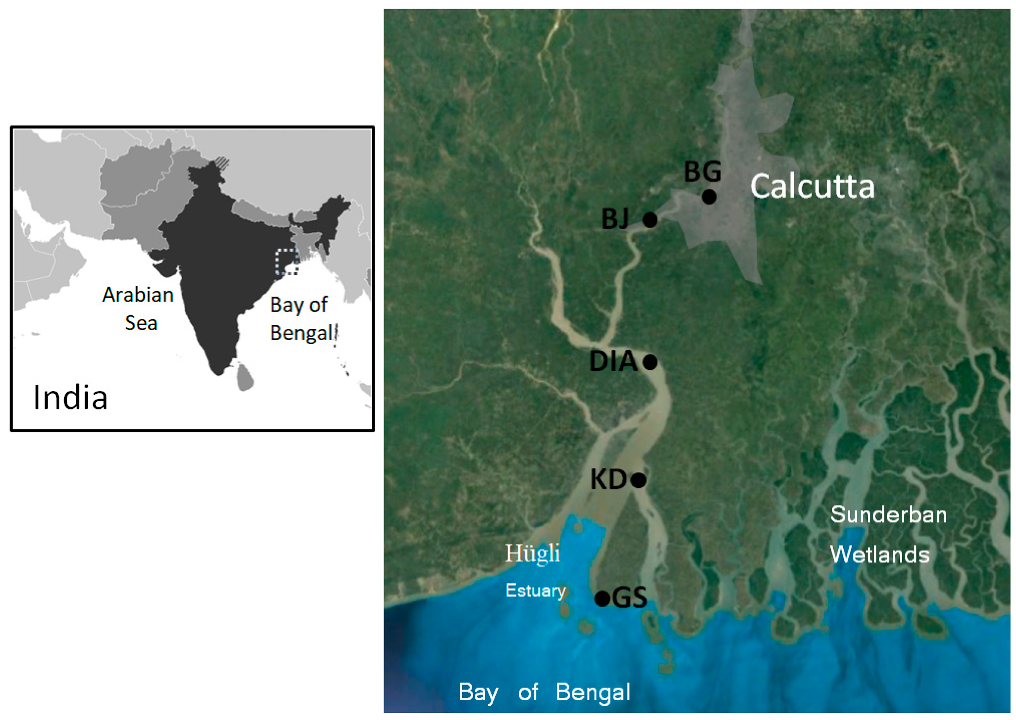
Station	Latitude	Longitude
GS (Ganga Sagara)	21°37′57.69″ N	88°4′14.77″ E
KD (Kakdwip)	21°52′47.67″ N	88°9′51.03″ E
DIA (Diamond Harbour)	22°11′14.73″ N	88°11′14.16″ E
BJ (Bajbaj)	22°29′23.20″ N	88°10′53.48″ E
BG (Babughat)	22°34′47.02″ N	88°20′48.93″ E

). The values for latitude and longitude were included in Table 1.

The station of Babughat (BG) is located nearby the city of Calcutta, which hosts around 4.5 million people and where the major sources of contamination are human activities, industrial and municipal discharges, car exhaust, chemicals used in agriculture, and the runoff caused by soil erosion due to deforestation [10]. The station Baj-baj (BJ) is located between the city of Calcutta and about 95 km from the mouth of the Ganges River Estuary. It hosts more than 76 thousand inhabitants. The quality of water in this area highly depends on seasonal and even circadian variations due to the intense tidal influences. The main sources of pollution are industrial wastes, pollution due to agriculture and aquaculture, domestic sewage, traffic, and mining discharges [11]. The station located in Diamond Harbour (DIA) is situated at 51 km south downstream Calcutta where the Ganges River turns into the Bay of Bengal, hosting more than 41 thousand inhabitants. At this point, the pollution is caused by discharges of untreated effluents from industries, agriculture, aquaculture, and domestic sources. The thermal power station Kolaghat Rupnarayan, located in a tributary of the Ganges, has a strong impact and pours directly into the Hügli River, North of Diamond Harbour [8]. Station Kakdwip (KD), with around 19 thousand inhabitants, is located just like Ganga Sagar in the Sundarban mangrove wetlands and usually suffers periodic flooding tide. This area is widely used for aquaculture of the tropical tiger shrimp Penaeus monodon [12]. Large amounts of metal ion are transported downstream and accumulate daily in the estuary, being deposited in the areas of Sundarban [13]. The station Ganga-Sagar (GS), also known as Sagar Island, is situated 150 km far from Calcutta; it has an extension of 300 km² and shelters 160 thousand people. It is subjected to strong anthropogenic stress and contamination from industrial and agricultural effluents [11]. Every year in January, thousands of people are concentrated in to have a Holly bath.

2.2. Sample Collection

Sediment samples were collected during summer period (June) using plastic tubes of 30 cm long and 5 cm diameter. The cores were collected by gently pushing the tube into the sediments and dug out, capped, and frozen on return to the laboratory. Each sediment core was sliced every 4 cm depth. Then, the sediments were dried in room temperature and sieved with a sieve of <2 mm fraction (ISO/DIS 11464). After that, the samples were transferred into zip locked polythene bags.

2.3. Analytical Procedure

The total organic carbon (TOC) content of sediment (<2 mm) was determined following the titration method described in Walkley and Black [14]. For metal analysis, approximately 100 mg of each sample was completely acid digested. The sample was transferred into a HP 500 vessel for total digestion; after that, 10 mL of deionized water (MilliQ water) was added. A mixture of 5 mL of HNO₃, 4 mL of HF, and 1 mL of HCl was also added. The vessels were then inserted into a microwave (CEM MARS 5) and heated at 100 °C for 1 h. The content of the pump was then evaporated to near dryness in Teflon vials (DigiPrep HotBlock, SCP Science), dissolved with 1 mL of double-distilled HNO₃ and 5 mL of Milli-Q water, heated for 20 min at 75 °C, and diluted with Milli-Q water [15]. The determination of Cd, Co, Cu, Ni, Pb, and Zn in the acid extracts was made with anodic stripping voltammetry using Metrohm equipment (VA 646) with Stand (VA 647). A hanging mercury drop electrode was used as the working electrode (Metrohm, 6.1246.020), together with a reference electrode of Ag/AgCl, KCl (3 M) (Metrohm, 6.0726.100) and an auxiliary electrode of Pt (Metrohm, 6.0412.100). The samples were degasified with N₂ and the preconcentration of the hanging mercury drop electrode was made at −1.1 V for 300 s. The scan was made from −1.075 to 0.050 V at −1 13.3 mV s. A differential pulse technique was used, with amplitude of 30 mV, duration of 40 ms, and periodicity of 0.3 s. Two millilitres of acetic/acetate buffer—(HAc/Ac) (NaAc, 1.73 M in KCl, 1 M) at pH 4.6 were added to each sample. The amount of buffer added was determined empirically to assure a uniform pH in the samples, regardless of the initial pH at which they were stored. The concentration of Hg was determined with a mercury analyzer LECO AMA-254. During the analysis procedural blanks and certified reference materials (MESS-3, PACS-2, and 1646a) were used. The recovery rate for the metals in the three reference materials was higher than 90% and average results are summarized in

Table 2. Recovery rate (%) for the metals analyzed in this study compared to the reference values using three reference materials (MESS-E, PACS-S and 1646a).

Metal(loid)	MESS-E	PACS-S	1646a
Ni	97.65	96.71	n.a.
Co	90.97	96.52	n.a.
Zn	94.97	96.70	97.75
Cd	97.92	99.28	98.65
Pb	97.63	93.44	91.45
Cu	95.28	98.38	98.3
Hg	98.90	98.68	n.a.

.

2.4. Data Treatment

One of the main processes controlling the incorporation of metals into the sediments and their subsequent migration to depth is the adsorption of metal to the sediment onto TOC. Spearman´s rank correlation tests were carried out with metal(loid) concentrations and TOC. The environmental risk factor was determined as the relationship between the average element concentrations per station in relation with the threshold effect level (TEL: concentration below which adverse biological effects are expected to occur rarely) determined by MacDonald et al. [16]. The original data set of each station and depth (included as mean values) including all the elements measured and the TOC were linked using an integrative approach [17]. The integration is based on a factor analysis that was conducted to explain the relationship observed between the initial set of variables and a smaller number of factors using principal component analysis (PCA) performed with the XLSTAT statistics software tool (2018.2). The analysis was performed on the matrix (varimax-normalized rotation), and a component-loading cutoff of 0.30 was used in the selection of variables for inclusion into the factors. Also, the same cut-off value (0.3) was used to select the factor that were significant in the study and that allow explaining more than 70% of the variance. The variables were auto-scaled (standardized) in order to ensure that they would be treated with equal importance.

3. Results and Discussion

The summarized element concentrations (Cd, Co, Cu, Hg, Ni, Pb, and Zn) in the sediments samples and their vertical distribution are given in

Table 3. Metal(loid) concentrations (mg/kg) and total organic carbon (%) in sediments in depth (cm) in the sampling’s stations (BG: Babughat; BJ: Baj-Baj; DIA: Diamond Harbour; KD: Kakdwip; GS: Ganga-Sagar) along the Ganges River and the Hügli Estuary.

Station	Depth	Ni	Co	Zn	Cd	Pb	Cu	Hg	TOC
BG	[0–4)	9.84	3.88	45.03	0.40	15.8	16.1	0.069	0.52
BG	[4–8)	7.79	3.56	21.47	0.40	11.8	13.8	0.033	0.56
BG	[8–12)	9.35	3.71	31.78	0.37	9.92	12.2	0.030	0.52
BG	[12–16)	7.41	2.88	24.07	0.36	11.0	10.9	0.030	0.63
BG	[16–20)	6.80	3.05	23.66	0.38	10.3	12.5	0.033	0.58
BG	[20–24)	13.6	3.73	23.04	0.44	8.05	11.5	0.026	0.49
BG	[24–28)	7.80	3.18	22.12	0.41	7.88	6.98	0.033	0.49
BG	[28–32]	8.35	3.72	21.07	0.25	7.62	10.9	0.140	0.12
BJ	[0–4)	9.77	4.42	23.73	0.26	9.36	9.13	0.057	0.15
BJ	[4–8)	9.97	4.23	26.22	0.15	7.01	9.08	0.051	0.09
BJ	[8–12)	9.46	3.91	28.40	0.14	7.43	8.68	0.050	0.15
BJ	[12–16)	9.16	3.92	15.08	0.36	4.03	6.85	0.031	0.49
BJ	[16–20)	9.84	3.75	31.20	bdl	11.2	9.40	0.022	0.49
BJ	[20–24)	10.8	4.13	38.14	0.20	11.5	3.86	0.029	0.42
BJ	[24–28]	14.2	3.98	28.14	bdl	10.3	5.94	0.029	0.51
DIA	[0–4)	9.52	4.33	26.51	bdl	7.30	15.0	0.022	0.58
DIA	[4–8)	19.9	6.12	49.20	bdl	8.11	15.3	0.023	0.53
DIA	[8–12)	9.62	3.80	18.67	bdl	6.40	7.36	0.027	0.48
DIA	[12–16)	10.1	4.40	26.02	bdl	8.98	10.5	0.021	0.48
DIA	[16–20)	15.1	5.42	23.96	bdl	7.70	7.67	0.018	0.46
DIA	[20–24)	15.4	4.30	27.90	bdl	6.67	7.10	0.019	0.50
DIA	[24–28]	12.5	4.29	22.93	0.24	5.54	5.44	0.023	0.53
KD	[0–4)	7.19	4.35	26.55	0.37	13.3	30.6	0.072	0.59
KD	[4–8)	8.91	4.65	31.64	0.30	12.5	21.2	0.041	0.67
KD	[8–12)	11.6	4.98	33.56	0.51	14.1	20.6	0.055	0.83
KD	[12–16)	7.90	4.90	22.68	bdl	12.0	19.5	0.032	0.69
KD	[16–20)	8.17	4.93	26.90	bdl	14.3	23.9	0.049	0.65
KD	[20–24)	7.99	4.62	21.74	bdl	11.5	15.7	0.042	0.63
KD	[24–28)	11.8	4.51	32.95	bdl	14.8	26.3	0.029	0.75
KD	[28–32)	12.6	4.33	35.47	bdl	16.2	20.2	0.032	0.61
KD	[32–36)	8.80	4.28	28.15	bdl	11.7	21.9	0.031	0.60
KD	[36–40]	10.4	5.27	31.49	0.41	16.0	31.6	0.028	0.58
GS	[0–4)	8.63	4.29	27.54	bdl	14.6	21.4	0.029	0.62
GS	[4–8)	8.45	4.74	26.81	bdl	14.2	19.8	0.027	0.68
GS	[8–12)	10.3	5.23	27.17	0.30	13.6	17.4	0.022	0.64
GS	[12–16)	10.7	5.35	24.92	bdl	12.2	11.6	0.024	0.62
GS	[16–20)	13.7	5.82	35.24	bdl	14.9	20.7	0.042	0.62
GS	[20–24)	9.13	4.72	19.43	bdl	9.33	13.1	0.043	0.64
GS	[24–28)	9.30	4.85	29.43	bdl	11.6	18.1	0.048	0.60
GS	[28–32)	7.79	4.03	21.72	bdl	11.6	13.8	0.032	0.61
GS	[32–36]	13.8	6.28	34.42	bdl	14.4	26.0	0.053	0.60

In bold values above threshold effect level (TEL in mg/kg) [16]: Ni = 15.9; Zn = 124; Cd = 0.68; Pb = 30.2; Cu = 18.7; Hg = 0.13. bdl: below detection limits.

.

The values measured for the TOC in sediments ranged between 0.4% and 0.9% with fluctuations with depth without a clear tendency. These values inform about a high variability in the area even at certain depth values such as those used in this study, and that is related to the high hydrodynamic that suffer the studied sites and to the different sources of contaminants.

Levels of organic matter in the sediments showed lower trends to estuarine sediments (1% of dry weight) [18]. There is an abnormally low value (0.09% TOC) in superficial layers (4–8 cm) in BJ. The TOC correlates most strongly (p < 0.01) with Pb and Cu (rs = 0.67 and rs = 0.72, respectively) and Co (rs = 0.47, p > 0.05). Element concentrations were higher associated with sediments with percentages of TOC between 0.5 and 0.8 % with an exponential tendency strongly determined for Ni, Co, Zn, and Cd (R² > 0.6).

Enrichment of element concentrations in bottom sediments represents a critical measure of health loss for any mangrove ecosystem [19]; however, said enrichment is not easily visible when comparing data from lowest layers and superficial ones (Table 3). The measured values of the different metals analyzed in this study do not clearly show a vertical distribution and are found different trends: higher concentration in deeper sediment than in surface sediments (e.g., Ni in BJ, DIA or KD, Pb in KD, Hg in BG). This kind of geochemical trend is related to the high hydrodynamic and contamination sources that exist in the area studied, including potential dredged operations. The average concentrations of the different metals analyzed in this study are ranged from high to low values as follows: Zn (28.2) > Cu (16.75) > Pb (11.5) > Ni (10.4) > Co (4.52) > Cd (0.16) < Hg (0.038).

Former studies have addressed this high dynamic situation: Abbas and Subramanian [20] calculated the annual sediment load about 729 Mt from sub-basin into the main basin and input to the Hügli Estuary, while annual transportation into the Bay of Bengal accounted about 328 Mt. Subramanian and Ramanathan [21] estimated the annual migration of sediment load carried by the upstream rivers (403–660 Mt). The hydrodynamic of the Estuary was further studied by Chatterjee et al. [19]. It is also possible to relate that some of the metal concentration and the organic carbon content in deeper sediments were higher than those measured in the surface of sediments due to past events of contamination. Higher depths than those used in this study will be necessary to confirm it and to distinguish between the high hydrodynamic as cause of the vertical profiles measured in this study.

All the concentrations analyzed for Ni, Co, Zn, Pb, and Cd were below the threshold effect level (TEL) values proposed as sediment quality guidelines by [16]. The metal Cu showed concentrations in the sediments located closer to the Hügli Estuary (KD and GS) that were higher and overpassed the TEL values proposed; furthermore, the ERF values (1.23 and 0.96, respectively) pointed a considerable risk for the environment. The station GS is the most sea influenced sampling site and could inform about the hydrodynamic influence in the distribution of this metal that probably is coming from the cities upriver. Moreover, the metal Ni shows higher values in the samples located at DIA station in Diamond Harbour, informing about potential sources of contamination in the area. Furthermore, there were measured values overpassing the TEL for Hg in the station BG upriver.

There is no clear pattern for longitudinal and vertical distribution of element concentrations. To address element concentration, organic carbon content, and vertical distribution relationships in the different studied sediments, a multivariate analysis (factor analysis) was conducted (

Table 4. Sorted (Varimax) rotated factor loadings of the original variables on the six principal factors for all depth (long monitoring) data set. The loadings >0.3 are highlighted in the table. Empty cells in the table are related to loadings lower than 0.3.

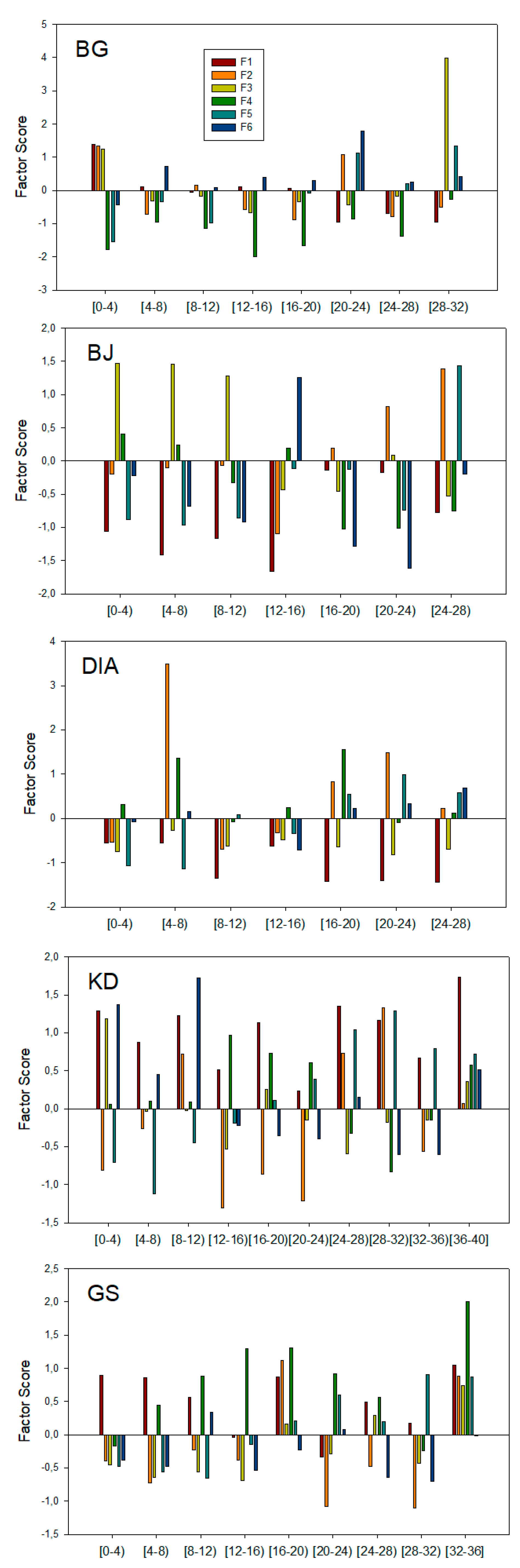
	F1	F2	F3	F4	F5	F6
%Variance	30.54	19.02	11.83	7.98	4.93	2.94
Depth	0.076	0.048	0.006	0.030	0.851	−0.084
Ni	−0.212	0.903	−0.171	0.364	0.204	0.094
Co	0.309	0.359	−0.039	0.899	−0.004	−0.045
Zn	0.452	0.772	0.086	0.005	−0.302	−0.246
Cd	0.045	−0.073	0.238	−0.490	−0.265	0.626
Pb	0.952	0.075	0.008	0.043	−0.005	−0.158
Cu	0.874	−0.045	0.092	0.308	0.024	0.168
Hg	0.098	−0.131	0.928	−0.034	0.024	0.119
TOC	0.656	−0.050	−0.641	0.122	0.116	0.226

) to group variables into factors. Unluckily, we do not have grain size characterization data available to corroborate the fluxes and hydrodynamic conditions in the studied area as pointed out by previous studies, therefore, due to the correlation established by TOC and the finest fractions of the sediments, it is assumed this longitudinal motion can be corroborated by the results using factor analysis.

There were six main factors identified that explain 77.24% of the total variance in the studied area (Table 4). The first principal factor (F1) accounted for 30.54% of the total variance. It accounts for the relationship between the metal distribution of Co, Zn, Pb, and Cu associated with the concentration of TOC. This grouping informs about a potential urban and hydrocarbon spillage process. In this sense, metals Cu and Zn are concentrated in the organic fraction of the sediments as supported for previous studies [22]. The vertical distribution of Zn and Pb in the different layers of the profiles from the Hügli Estuary was previously observed [19] and attributed to river input sediment properties and dredging [23]. In addition, Pb may be adsorbed over clay suspended particles and then deposited where it might be adsorbed preferentially over Zn²⁺ [13].

Factor 2 (F2), accounting for the 19.02% of the variance, represents the relationship between the Ni, Zn, and Co, as substitutes of Pb and Cu in the combustion of other types of hydrocarbon. It could be defined as representative of a combustion process related to distribution of these metals in the area studied. They are neither in relation to TOC nor depth. Moreover, the factor is in agreement with the relation Ni–Co and Ni–Zn as colloidal aggregation that was previously observed in the river [7]

The third factor (F3) accounts for 11.83% of the total variance. This factor is related to the distribution of Hg in a less approached Cd, clearly showing agricultural and industrial contamination processes and including old batteries as contamination sources. There is no geochemical relation to the depth, but it is an inverse relationship, greatly significant with the values of TOC measured in this study. This is a normal result because these elements do not keep usually a direct association with organic carbon.

Regarding factor 4 (F4), it accounts for the 7.98% of the variance and hosts the distribution of Co against the inverse concentration of Cd and is less significant with Ni and Cu. These associations are not related to depth and TOC. These metals’ relationship could be associated with the processes of antifouling paints for short and medium size boats in the area. The origin of the distribution of these metals could be related to this process.

The fifth factor (F5, 4.93% variance) represents sediment depth; it significantly informs about the absence of any relationship between the measured metal(loid)s, the organic carbon, and the depth. It is a process that informs that there is no vertical tendency in the distribution of metal(loid)s and TOC. This justifies the high hydrodynamic and high heterogeneity of samples. Furthermore, sediments up to 30 cm depth might be considered as superficial due to the lack of variability with depth (positive values in factor in Table 2).

Finally, the sixth factor (F6), accounting for 3.42% of the total variance, explains the Cd distribution with a slight correlation with TOC. This is a factor of individual distribution of metal Cd that includes a slight relation with TOC. The miscorrelation of Cd with the rest of the metal ions was also previously reported [7].

To confirm these associations and to identify the geochemical and contamination processes in each studied station, a representation of the factor scores previously defined and related to geochemical and contamination processes in each case study (stations) is showed in Figure 2. In the light of the analysis, it was found that BG, the most internal sampling site located closer to Calcutta, is a station with predominance of different processes (associated with the prevalence of the first three factors) in the most superficial layers: Urban discharges, agricultural-industrial contamination, and combustion of hydrocarbons. The sediments in this station are characterized by the heterogeneity of the sample and a complex distribution of metals not related to the depth. In the absence of a gradient of depth (F5 < 0), it can be confirmed there is no vertical variability. Due to the proximity to Calcutta, the association of some measured metals with TOC and strongly mixture of contamination sources is easily explained.

At station BJ, there is significant predominance of the distribution of metals (Hg and Cd) related to industrial activities, defined by F3. These contamination processes have been also identified by other authors in former studies [9]. There were not observed connections with TOC nor depth, reporting a high influence of the hydrodynamic (flood events) and marine tidal influence [19].

In the sediment in the area of the harbor (DIA), there is a complex mixture of geochemical and contamination processes as defined by the factor scores. There is a slight predominance of urban discharges defined by the predominance of factor 2 and the negative values of the industrial sources. Based on the location of this station, it is expected the mixture of processes measured that all are present there, confirming the high hydrodynamic and heterogeneity of the studied area.

There is a low and no-significant prevalence of urban contamination processes in sediments located in station BG, as informed by the low score values of F1 in Figure 2 for this station. Meanwhile, downstream there is a complex and significant prevalence of different geochemical and contamination processes in sediments collected in KD station. Different sources of pollution were identified (urban, agricultural, industrial) and there are geochemical associations based on the prevalence of factors in Figure 2. This fact can be related to the high hydrodynamic transporting influences from all other stations on these sediments. This is affected by all of them receiving sediments from all the upper stations, including tidal influence.

The lowest part of the estuary (sediments at station GS) is dominated by the prevalence of processes related to human activities, including urban discharges, represented by the positive prevalence of factors 1, 2, and 4 and by negative values in factors related to industrial sources of contamination (F3 and F6). Again, there is not a positive prevalence of the depth distribution that confirms the results obtained in this study and that is related to the heterogeneity of the vertical distribution of metals and TOC measured.

Anthropogenic inputs and natural processes may cause variation of metal concentration with the sediment depth. Anthropogenic inputs could increase or decrease with the time because transport of sediments in India and in tropical systems in general may vary irregularly with the weather (river floods, monsoon, etc.), as natural dynamic conditions. In addition, a migration of metal may occur in response to changes in the redox potential of sediments. Furthermore, it must be taken into account that benthic organisms may have a pronounced effect on metal vertical profiles due to bioturbation [24].

By comparing with previous studies in the area in the last four decades (

Table 5. A comparative account of metal concentration (in mg/Kg) measured in previous studies using sediments located in the same area than that showed in the current study.

Study	Ni	Co	Zn	Cd	Pb	Cu	Hg
This study	10.32	4.41	27.71	0.15	10.89	14.87	0.04
2018 [28]	1.65–68.35 a		11.04–127.98 a	0.06–0.29 a	1.62–58.29 a	2.37–59.47 a
2009 [19]		15.1 b	108 b	0.209 b	16.8 b	58.5 b
1999 [27]	16.8–58.3 b	4.5–15.5 b	27.2–95.1 b	0.11–0.69 b	6.83–14.2 b
1990 [22]	4–49 a		15–101 a			8–62 a
1987 [25]	20 a–32 b	22 a–36 b	46 a–71 b			21 a–26 b

^a Ganges River, ^b Hügli Estuary, ^c Bay of Bengal.

), element concentration results of the current study are below the range of element concentration in the Ganges River (Table 4). Subramanian et al. [25] determined the flux of metals from the estuary into the Bay of Bengal corresponds to freshwater supply. De et al. [26] also considered additional likely inputs from other smaller rivers draining from the petrochemical and metallurgical industrial belt of the hinterland. Ramesh et al. [27] found greater levels of Cd in the Hügli Estuary in association with rare earth elements (light and high) Pb and Ag with detrital material brought by the river and presence of V, Cr, Co, Ni, and Zn as estuarine processes and human input, as shown by F2 in the current study (Table 2). The results reported by Chatterjee et al. [19] a decade ago determined the concentration, distribution, and possible sources of trace elements in sediments at the confluence of the Ganges River and the Bay of Bengal. They reported mean values lower than other coastal regions in India in the Hügli Estuary, which bears severe anthropogenic stresses from commercial activities as also pointed out in the current study (F3 and F6 scores, Figure 2). Accordingly, in such research Cu, Ni, and Cr (Table 5) exceeded the effect range low concentration (ERL). Low Cd concentration values in sediments from the Ganges River were also found in the middle segment of the river by Jaiswal and Pandey [28]. Their study also found low values in sediment metal concentrations, but in contrast to current findings, they determined a low to moderate risk associated with different stations in the upper part of the river.

4. Conclusions

Element deposition follows natural processes especially associated with sediments with high concentration of organic carbon content. However, in coastal environments strongly impacted by human activity, industrialization, and urban sewages, such as the Hügli Estuary, metal concentrations in sediments can be elevated in the upper part. Nevertheless, the current study showed that in spite of the potential anthropogenic activities, natural processes such as flooding promote the dispersion of metal concentrations towards the sea, including the total absence of vertical profiles even for the organic carbon content. The metal(loid) association among them and with organic carbon significantly informs about heterogeneity in the sediment as a function of depth and about the absence of a vertical trend in their distribution. Moreover, these associations made possible to identify different sources of contamination mainly related to urban activities (metal association with the organic carbon content) and industrial activities (the distribution and association between Cd and Hg in the studied sediments). Only the Kakdwip area registered a potential environmental risk due to historical accumulation of Cu with levels above the threshold effect level proposed by the USEPA [16].

References

- Hakanson, L. Sediment variability. Sediment Toxicity Assessment; Lewis Publishers: Boca Raton, FL, USA, 1992; pp. 19–36. [Google Scholar]
- Chapman, P.M.; Wang, F. Assessing sediment contamination in estuaries. Environ. Toxicol. Chem. 2001, 20, 3–22. [Google Scholar] [CrossRef] [PubMed]
- Munksgaard, N.C.; Parry, D.L. Metals, arsenic and lead isotopes in near pristine estuarine and marine coastal sediments from northern Australia. Mar. Fresh Res. 2002, 53, 719–729. [Google Scholar] [CrossRef]
- Moore, J.W.; Ramamoorthy, S. Heavy Metals in Natural Waters: Applied Monitoring and Impact Assessment; Springer: New York, NY, USA; Berlin, Germany, 1983; 270p. [Google Scholar]
- Foster, I.D.L.; Charlesworth, S.M. Heavy metals in the hydrological cycle: Trends and explanations. Hydrol. Process. 1996, 10, 227–261. [Google Scholar] [CrossRef]
- Coleman, J.M. Brahmaputra River: Channel processes and sedimentation. Sediment Geol. 1969, 3, 129–239. [Google Scholar] [CrossRef]
- Sharma, Y.C.; Prasad, G.; Rupainwar, D.C. Heavy metal pollution of river Ganga in Mirzapur, India. Int. J. Environ. Stud. 1992, 40, 41–53. [Google Scholar] [CrossRef]
- Paul, D. Research on heavy metal pollution of river Ganga: A review. Ann. Agrar. Sci. 2017, 15, 278–288. [Google Scholar] [CrossRef]
- Sankla, M.S.; Kumari, M.; Sharma, K.; Kushwah, R.S.; Kumar, R. Heavy metal pollution of Holy River Ganga: A review. Int. J. Res. 2018, 5, 424–436. [Google Scholar]
- Guzzella, L.; Roscioli, C.; Vigano, L.; Saha, M.; Sarkar, S.K.; Bhattacharya, A. Evaluation of the concentration of HCH, DDT, HCB, PCB and PAH in the sediments along the lower stretch of Hugli estuary, West Bengal, northeast India. Environ. Int. 2005, 31, 523–534. [Google Scholar] [CrossRef] [PubMed]
- Sarkar, S.K.; Frančišković-Bilinsk, S.; Bhattacharya, A.; Sahaa, M.; Bilinsk, H. Levels of elements in the surficial estuarine sediments of the Hugli River, northeast India and their environmental implications. Environ. Int. 2004, 30, 1089–1098. [Google Scholar] [CrossRef]
- Ray, P. Aquaculture in Sunderban Delta—Its Perspective (An Assessment); International Books & Periodical Supply Service: Delhi, India, 1993; 197p. [Google Scholar]
- Guhathakurta, H.; Kaviraj, A. Effects of salinity and mangrove detritus on desorption of metals from brackish water desorption of metals from brackish water and shrimp. Acta Hydrochim. Hydrobiol. Banner 2004, 32, 411–418. [Google Scholar] [CrossRef]
- Walkley, A.; Black, I.A. An Examination of Degtjareff method for determining soil organic matter and a proposed modification of the chromic acid titration method. Soil Sci. 1934, 37, 29–37. [Google Scholar] [CrossRef]
- Caetano, M.; Fonseca, N.; Cesário, R.; Vale, C. Mobility of Pb in salt-marshes recorded by total content and stable isotopic signature. Sci. Total Environ. 2007, 380, 84–92. [Google Scholar] [CrossRef] [PubMed]
- MacDonald, D.D.; Carr, R.S.; Calder, F.D.; Long, E.R.; Ingersoll, C.G. Development and evaluation of sediment quality guidelines for Florida coastal waters. Ecotoxicol 1996, 5, 253–278. [Google Scholar] [CrossRef]
- DelValls, T.A.; Forja, J.M.; Gomez-Parra, A. The use of multivariate analysis to link sediment contamination and toxicity data to establish sediment quality guidelines: An example in the Gulf of Cadiz (Spain). Cienc. Mar. 1998, 24, 127–154. [Google Scholar] [CrossRef]
- Tanner, P.A.; James, J.W.C.; Chan, K.; Leong, L.S. Variations in trace metal and total organic carbon concentrations in marine sediments from Hong Kong. Environ. Technol. 1993, 14, 501–516. [Google Scholar] [CrossRef]
- Chatterjee, M.; Massolo, S.; Sarkar, S.K.; Bhattacharya, A.S.; Bhattacharya, B.D.; Satpathy, K.K.; Saha, S. An assessment of trace element contamination in intertidal sediment cores of Sunderban mangrove wetland, India for evaluating sediment quality guidelines. Environ. Monit. Assess. 2009, 150, 307. [Google Scholar] [CrossRef]
- Abbas, N.; Subramanian, V. Erosion and sediment transport in the Ganges river basin (India). J. Hydrol. 1984, 69, 173–182. [Google Scholar] [CrossRef]
- Subramanian, V.; Ramanathan, A.L. Nature of sediment load in the Ganges-Brahmaputra river systems in India. Sea-Level Rise and Coastal Subsidence; Springer: Dordrecht, The Netherlands, 1996; pp. 151–168. [Google Scholar]
- Jha, P.K.; Subramanian, V.; Sitasawad, R.; Van Grieken, R. Heavy metals in water and sediments of the Yamuna river (a tributary of the Ganga). Sci. Total Environ. 1990, 95, 7–27. [Google Scholar] [CrossRef]
- Singh, M.; Singh, I.B.; Müller, G. Sediment characteristics and transportation dynamics of the Ganga River. Geomorphology 2007, 86, 144–175. [Google Scholar] [CrossRef]
- Katz, A.; Kaplan, I.R. Heavy metals behavior in coastal sediments of southern California: A critical review and synthesis. Mar. Chem. 1981, 10, 261–299. [Google Scholar] [CrossRef]
- Subramanian, V.; Jha, P.K.; Van Grieken, R. Heavy metals in the Ganges estuary. Mar. Pollut. Bullet. 1988, 19, 290–293. [Google Scholar] [CrossRef]
- De, A.K.; Sen, A.K.; Karim, M.R.; Stockton, R.A. Pollution profile of the Damodar river sediments. Environ. Int. 1985, 11, 453–457. [Google Scholar] [CrossRef]
- Ramesh, R.; Ramanathan, A.L.; James, R.A.; Subramanian, V.; Jacobsen, S.B.; Holland, H.D. Rare earth elements and heavy metal distribution in estuarine sediments of east coast of India. Hydrobiologia 1999, 397, 89. [Google Scholar] [CrossRef]
- Jaiswal, D.; Pandey, J. Impact of heavy metals on activity of some microbial enzymes in the river bed sediments: Ecological implications in the Ganga river (India). Ecotoxicol. Environ. Saf. 2018, 150, 104–115. [Google Scholar] [CrossRef] [PubMed]