Article

A Spatially Explicit Comparison of Quantitative and Categorical Modelling Approaches for Mapping Seabed Sediments Using Random Forest

1
Department of Geography, Memorial University of Newfoundland, St. John’s, NL A1C 5S7, Canada
2
Geological Survey of Norway (NGU), Postal Box 6315 Torgarden, 7491 Trondheim, Norway
3
Department of Geography & Planning, 117 Science Place, University of Saskatchewan, Saskatoon, SK S7N 5C8, Canada
4
Ivany Campus, Nova Scotia Community College, 80 Mawiomi Place, Dartmouth, NS B2Y 0A5, Canada
*
Author to whom correspondence should be addressed.
Geosciences 2019, 9(6), 254; https://doi.org/10.3390/geosciences9060254
Submission received: 31 March 2019 / Revised: 24 May 2019 / Accepted: 3 June 2019 / Published: 6 June 2019
(This article belongs to the Special Issue Geological Seafloor Mapping)

Abstract

:
Seabed sediment composition is an important component of benthic habitat and there are many approaches for producing maps that convey sediment information to marine managers. Random Forest is a popular statistical method for thematic seabed sediment mapping using both categorical and quantitative supervised modelling approaches. This study compares the performance and qualities of these Random Forest approaches to predict the distribution of fine-grained sediments from grab samples as one component of a multi-model map of sediment classes in Frobisher Bay, Nunavut, Canada. The second component predicts the presence of coarse substrates from underwater video. Spatial and non-spatial cross-validations were conducted to evaluate the performance of categorical and quantitative Random Forest models and maps were compared to determine differences in predictions. While both approaches seemed highly accurate, the non-spatial cross-validation suggested greater accuracy using the categorical approach. Using a spatial cross-validation, there was little difference between approaches—both showed poor extrapolative performance. Spatial cross-validation methods also suggested evidence of overfitting in the coarse sediment model caused by the spatial dependence of transect samples. The quantitative modelling approach was able to predict rare and unsampled sediment classes but the flexibility of probabilistic predictions from the categorical approach allowed for tuning to maximize extrapolative performance. Results demonstrate that the apparent accuracies of these models failed to convey important differences between map predictions and that spatially explicit evaluation strategies may be necessary for evaluating extrapolative performance. Differentiating extrapolative from interpolative prediction can aid in selecting appropriate modelling methods.

1. Introduction

There is growing pressure on marine ecosystems due to human use, especially near coasts where interactions between terrestrial and marine drivers have the potential to generate large cumulative impacts [1]. Coastal ecosystems provide many important goods and services to both coastal and inland inhabitants [2,3,4]. Therefore, it is often necessary to balance competing demands from stakeholders with the sustainable management of marine resources and ecology [5]. Marine spatial planning (MSP) is a framework by which this can be accomplished [6]. Using MSP, local maps of ecology are analyzed alongside those of human use to identify overlaps and conflicts. This spatial information is used to implement management plans for the current and future use of the marine system [6]. Maps are, therefore, key components to such management initiatives as the primary means of conveying spatial information.
Seafloor substrate maps are particularly useful for determining the distribution of coastal marine biota. Substrate composition can be a strong predictor of benthic biodiversity [7]. The presence of hard substrata, for example, can provide attachment surfaces for sessile animals, marine algae, and the grazers that feed on them, while soft sediments provide habitat for many infaunal invertebrates [7]. Substrate composition also determines seabed complexity by providing structure and shelter for marine fauna—factors that correlate with biodiversity [8]. Substrate maps can therefore inform on the distributions of single species or biodiversity—both of which may be important components of a given management framework.
A variety of methods for producing seabed sediment maps have been explored (e.g., [9,10,11]). Surficial sediment maps were traditionally produced by manual interpretation of ground-truth data in the context of local geomorphology and often, sonar data (e.g., Todd et al. [12]) but modern methods increasingly rely on automated objective approaches [13]. These have recently become feasible thanks to the widespread accessibility of digital data, powerful geographic information system (GIS) tools and high-performance computing – they allow for mapping a range of substrate characteristics. Grab sample and core data, for example, have been used to predict sediment grain size [10,14] and particulate organic carbon content in unconsolidated sediments [15], while the presence of rock or hard substrates has been predicted from underwater video [16,17]. There are now a variety of approaches to choose from for a given mapping application and it is important to select those that fit the given geographic and dataset characteristics.
Coupled with high-resolution acoustic mapping, automated statistical methods are among the most promising recent approaches to mapping seabed sediments. They perform well compared to other methods [9,18] and are objective—providing several advantages over manual or subjective approaches [19]. In supervised modelling, ground-truth sediment samples (e.g., grabs, cores, video observations) are used to train a statistical model based on environmental data (e.g., depth, seabed morphology, acoustic seabed properties). Statistical relationships between sediment samples (response variable) and environmental data at the sample location (explanatory variables) are used to predict sediment characteristics at unsampled locations. With spatially continuous remotely sensed environmental data, it is therefore possible to produce full-coverage seabed sediment maps from relatively sparse sediment samples.
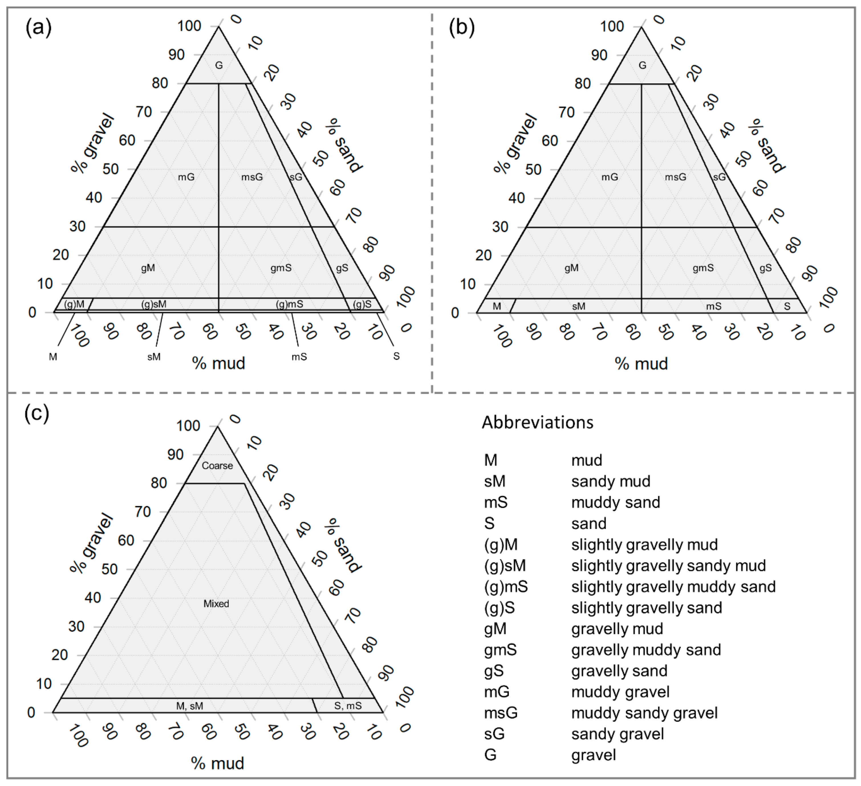
For producing classified (thematic) maps of sediment grain size, several common textural classification schemes, such as Folk [20], place grain size samples on a ternary diagram according to the ratio of sand:mud and the percentage of gravel (Figure 1a). Similar textural schemes coarsen the thematic resolution of Folk’s by aggregating to fewer classes, such as the British Geological Survey (BGS) modification for small-scale (1:1,000,000) maps, which eliminates the “slightly gravelly” classes (Figure 1b; [21]). To account for substrate types used in the European Nature Information System (EUNIS) habitat classification, a further simplified version of Folk’s classification with only four classes has been suggested and is widely used [21,22] (Figure 1c). Among other criteria, the selection of a classification scheme may be for compatibility with regional management systems (e.g., EUNIS [23,24]), for alignment with existing literature [25] or for matching with ground-truth data.
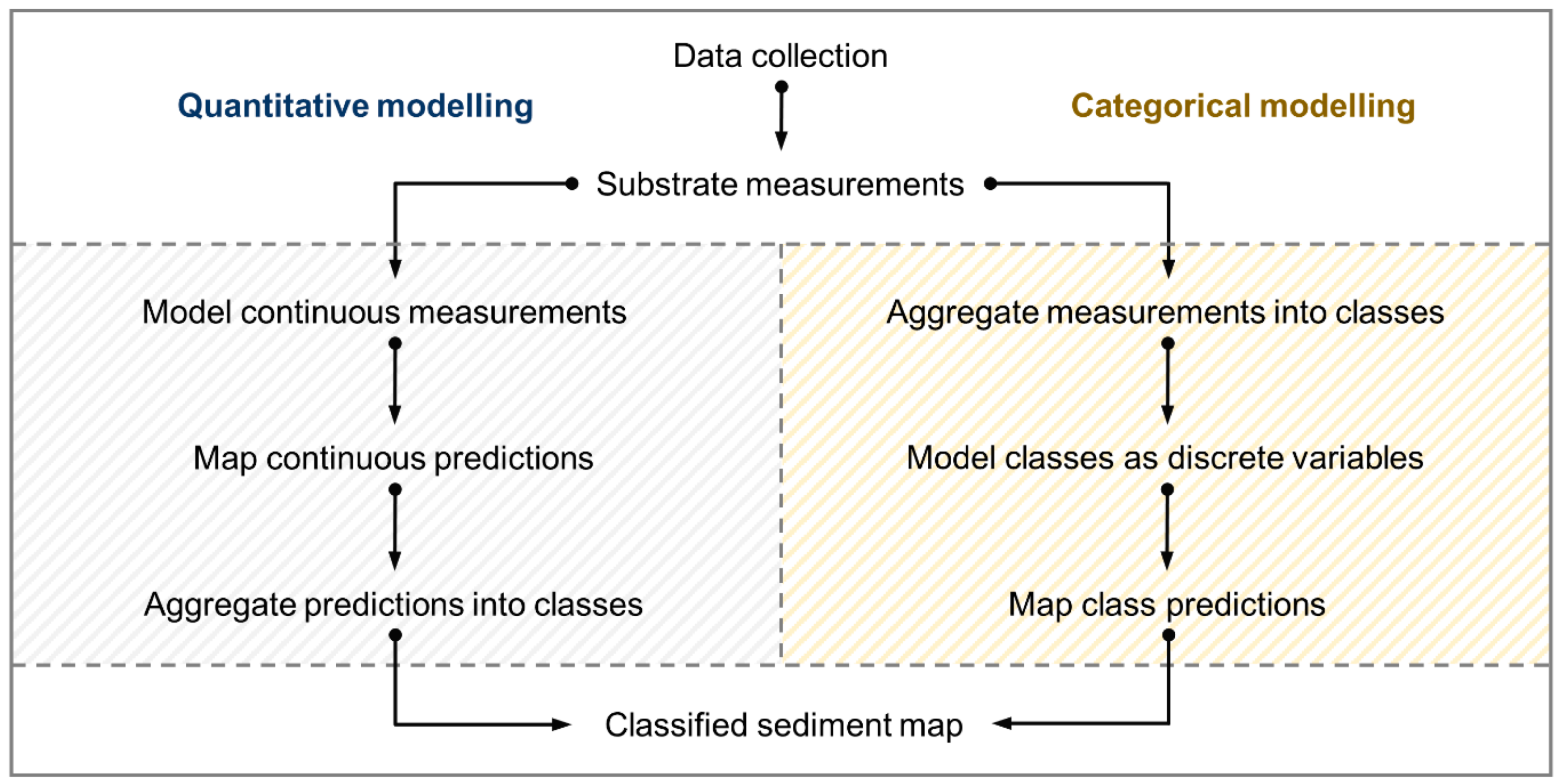
Using a supervised modelling approach, ground-truth sediment data are commonly treated in two ways to produce classified maps of seabed sediment according to schemes such as those described in Figure 1:
1. Quantitative measures of a substrate property, such as grain size fraction (e.g., percent mud, sand, and gravel), are used to predict quantitative gradational values across the full environmental data coverage (e.g., [26]). These predictions are useful for management or further modelling but some applications require classified or thematic maps, which can be produced by classifying the quantitative predictions according to some scheme (e.g., Figure 1). This is useful for summarizing sediment composition in a single map or for ensuring compatibility with regional management plans or similar research (see Strong et al. [25] for discussion of classification and compatibility).
2. Ground-truth data are aggregated according to a classification scheme prior to modelling, thereby treating them as categorical variables (e.g., [27]). It may also be the case that inherited data (e.g., from the literature, online databases, legacy data) are already classified and the quantitative data are unavailable or that datasets consist of sediment classes derived from visual assessment. In these cases, the options available to the modeler are limited and the categorical classification approach may be the logical choice. Using this approach, a model can predict the occurrence of the observed classes over the full extent of the environmental data.
Here we will refer to these as “quantitative” and “categorical” modelling approaches. While the quantitative approach is also known as “continuous” or “regression” modelling and categorical is commonly referred to as “classification,” we use the terms “quantitative” and “categorical” to reduce confusion, since the other terms also have other meanings that are relevant here (e.g., “classified” maps can be produced from either approach and all predictions are “spatially continuous”).
Each of these broad approaches contain numerous individual modelling techniques with their own intricacies, many of which have been compared in the ecological and conservation management literature (e.g., presence-absence models [28], regression models [29], machine learning [30], geostatistical and hybrid methods [18,31]). Among machine learning techniques, Random Forest [32] is a particularly flexible and accurate method that is capable of both quantitative and categorical modelling. This flexibility, coupled with widespread availability via popular statistical and GIS software (e.g., R, ArcGIS), has made Random Forest popular for seabed mapping. Given the goal of producing a classified (i.e., “thematic”) seabed map using continuous sediment data, Random Forest could be applied using either quantitative or categorical approaches (Figure 2) at the discretion of the user.
There are apparent advantages and disadvantages to both quantitative and categorical sediment modelling approaches for producing classified maps. Unclassified quantitative predictions on their own constitute a useful result for further modelling and mapping and are flexible once produced—it is easy to classify and reclassify quantitative values as necessary. The modelling process can be complex though, potentially involving data transformations such as additive log-ratios for compositional data [33], multiple models for different log-ratios [26] and multiple corresponding tuning and variable selection procedures. On the other hand, the categorical modelling procedure can be more straightforward, requiring little data manipulation once ground-truth measurements have been aggregated into classes and explanatory variables have been selected. Class labels can be predicted to new data relatively easily. Once produced though, classes are more static compared to quantitative predictions. It may be possible to simply aggregate mapped classes to a more general scheme (e.g., Folk to simplified Folk; Figure 1) but it may also be necessary to re-classify the ground-truth, select new variables and re-tune model parameters for a new classification, especially if the original scheme is a poor match for the data.
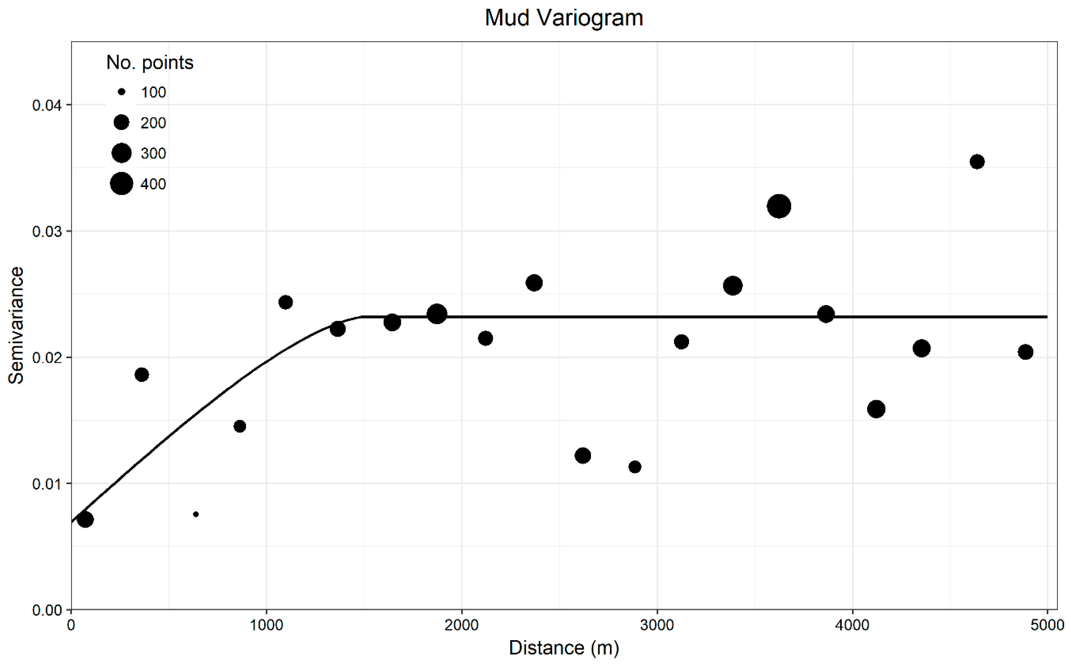
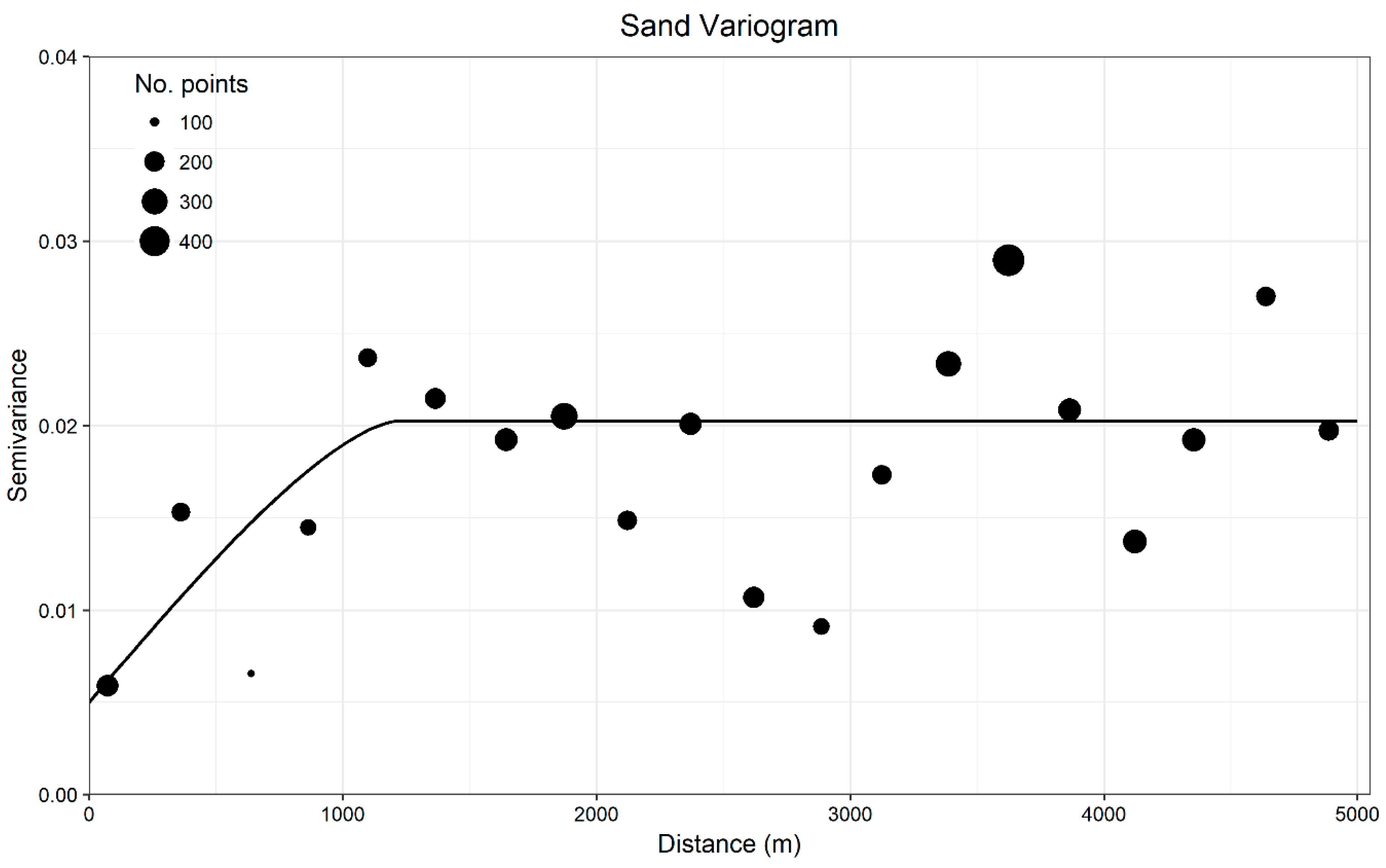
Otherwise, characteristics of the ground-truth data and the type of prediction required by the models may be important qualities for determining the suitability of modelling approaches. For example, sample size, distribution and bias, class prevalence and spatial dependence are known to have profound effects on the performance of distribution models [29,34,35] and particularly Random Forest [36]. These and other dataset characteristics might influence the appropriateness of the approach selected for producing classified maps. For instance, rare classes may be difficult to model using a categorical approach when they have been sampled few times but may cause less of an issue when modelled as quantitative variables. In some cases, clustered or uneven sampling may create spatial dependence in the response data [37], violating assumptions of independence [38]. This could have unintended consequences for prediction and apparent model accuracy, especially when extrapolating to new locations [37,39] and these could depend partly on the modelling approach. Here we refer to extrapolation in a spatial sense as predictions outside of the sampled area, whereas interpolation occurs between sample locations. An implicit assumption then, is that interpolation operates within the sampled environmental conditions, while extrapolation may predict outside of them.
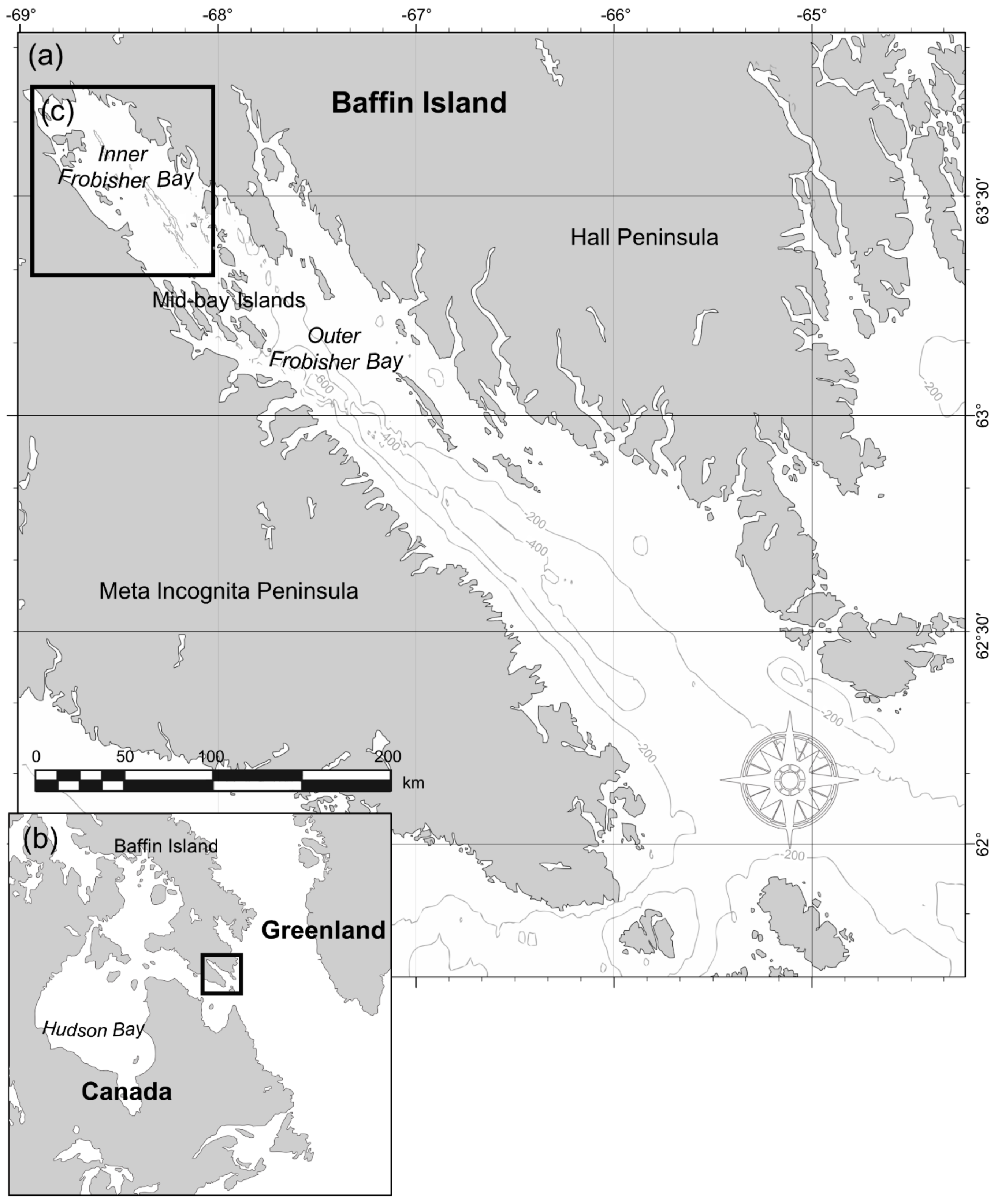
The primary goal of this study was to create a classified seabed sediment map for inner Frobisher Bay, Nunavut, Canada from grab samples and underwater video using the Random Forest statistical modelling algorithm. Ground-truth characteristics, however, suggested that spatial dependence might be an issue when extrapolating seabed sediment characteristics to unsampled locations and evaluating these predictions. We therefore undertook a spatially explicit investigation of the qualities of the two modelling approaches—quantitative and categorical (Figure 2) —for predicting sediment grain size classes from grab samples using Random Forest. Coarse substrates that were not adequately represented in grab samples were modelled separately using underwater video data and the two predictions were subsequently combined to produce a single map of surficial sediment distribution.
Specifically, when evaluating the quantitative and categorical Random Forest models for producing classified maps, we investigated: (1) their performance when extrapolating grain size predictions to new locations and if this was affected by spatial autocorrelation; (2) the appropriateness of three levels of classification based on the relative proportions of grain size measurements; and (3) if the two approaches produced similar maps. Because the observations of coarse sediment from video transects were likely to be spatially autocorrelated, we investigated if the proximity of these samples: (1) inflated the apparent accuracy of coarse substrate predictions; and (2) caused overfitting in model training. The results of these investigations informed the selection of modelling approach, while also providing spatially explicit accuracy estimates. Based on the results, we provide recommendations on the utility and potential pitfalls of these approaches in a spatial context.

2. Materials and Methods

2.1. Study Area

Frobisher Bay is a long (~265 km), northwest-southeast-oriented macrotidal fjord located in southeastern Baffin Island, Nunavut, Canada (Figure 3). It can be partitioned into two morphologically distinct sections. The inner part spans from the northwest head of the bay to the mid-bay islands, with a maximum depth of approximately 350 m. Much of this section is shallow (< 100 m) with extreme tides (> 10 m) resulting in extensive tidal flats. The mid-bay islands separate the predominantly muddy shallow inner bay from the coarse and bedrock-dominated outer bay, which deepens to over 800 m and opens to the North Atlantic. The southwest coast of the outer bay is the fault boundary of a half-graben and is characterized by steep rock cliffs.
This study focuses on inner Frobisher Bay. The morphology and orientation of submarine features here are a product of repeated Quaternary glaciations, the most recent of which receded between 9-7 ka BP [40,41]. These have produced a complex, heterogeneous seabed, with erosional and depositional glacial features such as scour troughs and moraines indicative of northwest-southeast ice flow. Currently, seabed sediments are re-mobilized by several non-glacial processes, including tidal currents, submarine slope failures and iceberg and sea-ice scour [42].

2.2. Environmental Data

Multibeam echosounder (MBES) bathymetry and backscatter data (Figure 4 and Figure 5) were collected between 2006 and 2017 to characterize the seabed as part of the ArcticNet project “Integrated Marine Geoscience to Guide Environmental Impact Assessment and Sustainable Development in Frobisher Bay, Nunavut” [42]. The CCGS Amundsen collected opportunistic MBES data during transit to and from Iqaluit between the years 2006–2008 with a Kongsberg EM300 30 kHz echosounder and between 2009-2017 with an EM302 (30 kHz). The RV Nuliajuk completed targeted surveys in the bay between 2012–2013 with an EM3002 (300 kHz) and between 2014–2016 with an EM2040C (200–400 kHz). Details on MBES data processing are included in Appendix A.

2.3. Ground-Truth

Ideally, a sediment model would rely on a single consistent source of ground-truth data, yet grab samples commonly fail to accurately represent coarser sediments [45,46], while it can be difficult to consistently distinguish mud from sand in underwater video [47]. To overcome these limitations, we modelled finer grain sizes (< 4000 μm) using grab sample data and coarse substrates (≥ 4000 μm; that is, pebble, cobble, boulder) from video observations.
Grab samples (n = 239) and underwater video (n = 78) were collected in 2015 and 2016 to provide substrate ground-truth for the MBES data (Figure 4 and Figure 5). Ground-truth sites were selected from the area of MBES coverage prior to each field season using a random approach, stratified by water depth up to 200 m and seabed slope. Because sampling and mapping occurred simultaneously, only part of the final mapped area was available for sample site selection each year, resulting in unsampled areas.
A live-feed Deep Blue Pro underwater camera with a GoPro Hero4 was deployed at each selected site to collect high-definition video for a four-minute drift. Two lights were attached to the camera mount to illuminate the seabed and two green lasers, spaced 5 cm apart, were attached for scale. Positioning was obtained using a Garmin 18x PC GPS with video overlay, providing coordinates at the surface for the duration of the recording. GPS accuracy was rated at < 3 m and though efforts were made to keep the location of the GPS above the camera during drifts, it is likely that the locational error was greater under windy or high-current conditions due to horizontal drift of the camera from the vessel, especially at the greatest depths. Positional error potentially exceeded 10 m under high-drift conditions; if this was suspected, the drift was cut short. Still frames were extracted for analysis every 10 s for the duration of the video. If coarse substrates (pebble, cobble, boulder) were visible in a frame, they were labelled as “present.” All observations were aggregated so that coarse substrates were labelled as “present” or “absent” for each 10 m raster cell that was sampled.
Up to three sediment samples were collected from the area near each site using either a 24-l Van Veen or a 2.4-l Petite Ponar grab and individually georeferenced from the surface using the ship’s GPS location. Each grab sample was sub-sampled for ~100 g of sediment, which was considered sufficient for measuring grain size composition up to 4000 μm. These were stored in a sample jar and frozen for transport. In the lab, samples were thawed and dried at low heat in an oven. Samples were dry-sieved for 5 min in a mechanical sieve shaker to separate mud (< 63 μm), sand (63–2000 μm) and gravel (2000–4000 μm) fractions. Many samples had a high proportion of flocculant mud that failed to disperse during dry sieving. To obtain an accurate measure of the mud fraction, samples were gently spray-rinsed through a 63 μm sieve and agitated by hand, washing away the mud fraction. The remaining sediments coarser than 63 μm were re-dried and weighed to estimate the proportion of mud that was lost. The weights of each fraction were divided by the total weight to obtain percent mud, sand and gravel composition.

2.4. Statistical Modelling

The Random Forest machine learning algorithm was used to model both sediment grain size and presence of coarse substrates. Random Forest is an ensemble modelling method that uses bagging [48] to combine the results of many individual classification or regression trees, whereby many bootstrap samples of the modelling dataset are drawn and a decision tree is fit to each [32]. A random set of predictor variables is selected to partition the data at each decision tree node and the data not selected for a given bootstrap sample (termed “out-of-bag” observations) are predicted by the decision tree. This provides several useful metrics, such as (1) a predicted class or value for each observation based on majority vote, (2) estimates of accuracy that are comparable to cross-validation and (3) estimates of variable importance (see Cutler et al. [49] for explanation in an ecological context) and these can be used to evaluate the quality of the model.
Because Random Forest is an ensemble of decisions trees, it is generally considered robust to noisy or unimportant predictors [32,50]. Large numbers of quantitative and categorical variables can therefore be included in the model and non-linear responses are automatically modeled with interaction (a quality of decision trees). Furthermore, it can perform both quantitative and categorical modelling (e.g., Figure 2). These qualities have made Random Forest popular for environmental modelling, yet the resulting ensemble of trees is complex, making it difficult to understand exactly how model predictions are derived. Ways in which variables interact in the model, for example, is difficult to know given that interactions can be multiple levels deep for each decision tree, of which there are hundreds or thousands. Though this complexity makes Random Forest a powerful predictor in the range of sampled conditions, it may be less effective at extrapolation [51,52], especially for rare classes. This is sometimes alleviated by subsampling the sample dataset to ensure equal class observations, yet this method can potentially cause rare classes to be overpredicted [36]. These qualities must be considered when evaluating the suitability of Random Forest for a given modelling application.
For the categorical grain size modelling approach, samples were assigned class labels according to three ternary schemes prior to modelling to test different levels of data aggregation. The Folk [20] and simplified Folk schemes were used according to Long [21]. Here, the “slightly gravelly” boundary for the Folk classification is at 1% rather than “trace,” as in Folk [20]. The third classification was simply “muddy” or “sandy” if there was a majority of either size fraction. This was used instead of the EUNIS simplification to the Folk classification (Figure 1c), which was not appropriate given the data – most samples were muddy and < 5% gravel. The EUNIS simplification would aggregate nearly all the samples into the class “mud and sandy mud.”
For the quantitative approach, percent mud, sand, and gravel measurements were transformed to an unbound additive log-ratio (ALR) scale [33] with respect to the mud fraction:
A L R s m = log 10 ( S M )
A L R g m = log 10 ( G M )
where ALRsm and ALRgm are the additive log-ratios of sand to mud and gravel to mud and M, S, and G are the proportions of mud, sand, and gravel size fractions measured in a grab sample, respectively. Note that the results are unaffected by the choice of size fraction to serve as the denominator [53]. Model predictions were then back-transformed to a compositional scale bound between 0 and 1, corresponding to the relative percentage of each size fraction and summing to 1 for each sample [54]:
S = 10 ( A L R s m ) 10 ( A L R s m ) +   10 ( A L R g m ) + 1
G = 10 ( A L R g m ) 10 ( A L R s m ) +   10 ( A L R g m ) + 1
M = 1 ( S + G )
To produce a classified map from the quantitative output, predictions were classified according to the three ternary schemes above.
The presence or absence of coarse substrates was recorded for each underwater video still frame to produce binary presence-absence data. These were used to train a categorical Random Forest model, essentially treating the presence or absence of coarse substrates as a two-class categorical response. Random Forest can output class probabilities rather than the class of majority vote, which allows the presence threshold to be tuned according to the classification goal, rather than the arbitrary default value of 0.5. Though tuning this threshold cannot solve the problem of poor model fit, it can potentially increase the efficiency of meeting explicit predictive goals for a binary classifier (such as balancing correctly classified presences and absences or accurately predicting a certain sediment class), especially when model prediction and performance are highly sensitive to class prevalence [55].

2.5. Explanatory Variables

In addition to the primary MBES data (bathymetry and backscatter), 11 secondary variables were tested for inclusion in each of quantitative and categorical grain size models and the coarse substrate model using a multiscale approach ([56]; Appendix B). Five bathymetric derivatives that describe most of the topographic structure of a surface suggested by Lecours et al. [57] were calculated using their toolbox for ArcGIS (the eastness and northness of seabed slope aspect, relative difference to the mean bathymetric value, slope, local bathymetric standard deviation; [58]). Local bathymetric standard deviation was omitted because it was highly correlated with seabed slope but did not perform as well. Three measures of surface curvature (total, plan, profile) were derived using the “Curvature” tool in ArcGIS Pro v.2.2.3 and two measures of surface complexity (surface area:planar area [SA:PA], vector ruggedness measure [VRM]) were derived using the Benthic Terrain Modeler toolbox [59] for their potential as topographic surrogates that influence bottom currents and potentially sediment transport. The range of backscatter values in a circular neighborhood and their standard deviation (SD) in a 3 x 3-pixel neighborhood were derived for each spatial scale as potential surrogates for local substrate variability. The Euclidean distance to the nearest coast was calculated as a potential predictor of sediment grain size based on transport distance from terrestrial sources.
Random Forest is generally considered robust to noise, ignoring unimportant predictors, yet there are benefits to variable reduction such as decreased variability between model runs and more accurate estimates of error [36]. We simplified the predictor set by removing variables that had Spearman’s ρ ≥ 0.70—a common threshold for reducing correlated variables (e.g., [60,61,62]; Appendix B).

2.6. Evaluating Model Performance

All predictions were first tested using a leave-one-out cross validation (LOO CV). Using this approach, a single sample is removed from the dataset and all other samples (N-1) are used to train the model. The class of the withheld sample is then predicted using the N-1 model. This is repeated for every sample in the dataset, producing observed and predicted classes at every sample location, which are used to estimate predictive performance. Error matrices were computed to observe the success in predicting the observed classes. From this we derived the percent correctly classified and the kappa coefficient [63]. Percent correctly classified is simply the proportion of test samples that were assigned the correct label. Kappa is a statistic that reflects whether the model achieved better results than to be expected at random and is calculated from
κ = p o p e 1 p e
where κ is the value of kappa between −1 and 1 (with 0 describing predictions that are no better than random), p o is the proportion correctly classified and p e is the proportion correctly classified due to chance, based on the frequency of observations and predictions of each class. Because the performance of the coarse presence-absence model depends on the probability threshold, the threshold-independent area under the receiver operating characteristic curve (AUC), which is the plot of sensitivity against 1-specificity [64] and the maximum kappa values at all thresholds (e.g., [28]) were used to compare candidate models.
Spatial autocorrelation is known to inflate estimates of predictive performance [36,65]. To determine its effects on the modelling approaches tested here and whether models were able to extrapolate to unsampled locations, we also conducted a spatial leave-one-out cross-validation (S-LOO CV) [66]. This procedure is identical to LOO CV, except that a spatial buffer is placed around the withheld test point and training data from within this buffer are omitted from both model training and testing so that there are no training data proximal to the test. This aims to eliminate spatial bias in accuracy assessment by removing points that are spatially autocorrelated with the test site up to the specified buffer distance.
We calculated empirical variograms for the observed grain size values and coarse substrate observations to determine a suitable buffer distance. We used the variogram model range to estimate the distance beyond which the effects of autocorrelation are negligible. This distance has been suggested as adequate for S-LOO CV [67]. Variograms were calculated up to 5000 m and multiple models were tested for characterizing the major range using the Geostatistical Wizard in ArcGIS Pro v.2.2.3.
The coarse substrate model was trained using image frames from video transects and these were expected to be highly autocorrelated due to their proximity. Therefore, in addition to the above two assessment procedures, we conducted a spatially resampled leave-one-out cross-validation (SR-LOO CV) to determine whether this spatial dependence affected model fitting in addition to performance estimation. Because Random Forest is an “embarrassingly parallel” algorithm [50], separate “forests” can be combined and treated as a single model to make predictions. The SR-LOO CV builds on S-LOO CV by using the same spatial buffering procedure (i.e., the withheld test sample is spatially buffered; points within the buffer are excluded from training and testing), except that each training point for each “leave-one-out” iteration is also spatially buffered, so that no adjacent points are used for model fitting or testing (similar to the algorithm in Holland et al. [68]). Because this severely limits the number of samples available for training each iteration of Random Forest, we can randomly subsample each “leave-one-out” training dataset many times (100 here) to acquire different subsets of spatially independent training data. By producing only a small number of trees (ntree) from each of the 100 spatially independent data subsets, it is possible to achieve the same number of trees in a forest that are desirable in a full “leave-one-out” iteration (e.g., ntree = 2000 here). This effectively creates the same number of trees as in a normal Random Forest run but produces the “forest” using the combination of many small, spatially independent subsets, rather than the full dataset.
The results of these cross-validations were analyzed to address the goals of this study. For grain size predictions, we first investigated the performance of the quantitative and categorical approaches to determine if these models could successfully extrapolate sediment grain sizes at unsampled locations and whether spatial autocorrelation interfered with assessing map accuracy. Performance was assessed using multiple classification schemes at different levels of grain size detail (i.e., aggregation) to select one that fit the data. We then compared maps produced using both approaches to determine if and how any differences in model performance manifested in the mapped predictions and if the maps agreed. For predicting the presence of coarse substrates, we tested whether the proximity of sample points within video transects inflated estimates of predictive performance and also whether their proximity caused overfitting of Random Forest models.

2.7. Map Prediction

Predictions of sediment grain size and the presence of coarse substrates were combined to produce a single map of seabed sediment distribution. The results from the accuracy assessments and map comparison, and also the qualities inherent in the two modelling approaches, were used to select a suitable model for predicting sediment grain size classes. The probability of coarse substrate presence was predicted for the entire study area. To combine these predictions with those of grain size, an occurrence threshold was set to maximize the sum of sensitivity and specificity, which aims to balance the class accuracy of predictions [60] and which has been demonstrated to perform well compared to other threshold selection criteria [55]. Thus, the combined map predicts the sediment grain size class and whether coarse substrates are present for each pixel throughout the study area (e.g., “muddy with coarse substrate”).

3. Results

3.1. Grain Size Data

The sampled substrates were primarily muddy, with some sandy sediments (Figure 6). When classified according to Folk [20], the most common class was (g)sM (40.72%), followed by sM (38.14%) and (g)mS (13.40%). The simplified Folk scheme eliminates the “slightly gravelly” modifier, aggregating the classes (g)sM and (g)mS with sM and mS, increasing these class proportions to 78.87% and 18.04%, respectively. In the “muddy/sandy” classification, 79.38% of samples fall into the “muddy” class, with the remaining 20.62% in “sandy.” Coarse substrates were observed in 20.06% of raster cells containing underwater video observations (e.g., Figure 7; Table 1).

3.2. Spatial Autocorrelation

Estimates of major range from the Geostatistical Wizard variogram models were used to determine a buffer distance for the spatial leave-one-out cross-validations. Circular variogram models provided a distinct major range compared to the more asymptotic models (e.g., exponential, Gaussian, Bessel), were relatively stable with varying input parameters and fit the data comparatively well. The major ranges of the circular mud and sand variogram models were 1497 m and 1210 m, respectively, when calculated at a maximum distance of 5000 m (see Appendix C). There appeared to be little change in gravel measurement variance with increasing distance and they did not yield a useable variogram model. We selected a buffer distance of 1500 m for the S-LOO CV based on the mud and sand major range estimates. The major range of the circular coarse substrate model was 199 m; we selected a buffer distance of 200 m for S-LOO CV and SR-LOO CV methods based on this model.

3.3. Variable Selection

Different sets of scale-dependent variables were selected for modelling ALRsm, ALRgm, grain size classes, and the presence of coarse substrates (Table 2 and Table 3). Backscatter range was commonly correlated with the backscatter standard deviation (SD) (ρ ≥ 0.70) and only one of these two variables was generally selected, except in the classification model where the correlation between backscatter range at 250 m scale and backscatter SD at 100 m scale was below this threshold. The different curvature measures were often correlated at similar scales and also to RDMV. Total curvature was correlated with one of these variables at every scale tested and consistently had a weaker relationship with the response—it was therefore removed from all models. The two measures of complexity, SA:PA and VRM, were also correlated at similar scales.

3.4. Grain Size Model Evaluation and Comparison

The LOO CV suggested that the simplified Folk and muddy/sandy classes were predicted accurately, with predictions from the categorical approach generally more accurate than the quantitative, while Folk classes were not predicted accurately using either approach (Table 4). The error matrix shows that this poorer performance was the result of several uncommon Folk classes that were not successfully predicted (Appendix D); the categorical Folk predictions had a percent correctly classified of 54.64% and predictions that were only marginally better than random ( κ = 0.25). The greater accuracies of the simplified Folk and muddy/sandy schemes is a product of rare classes being aggregated into broader ones, reducing their misclassification. Though the quantitative approach was generally less accurate than the categorical using LOO CV with all schemes, it was similar in that the simplified schemes were predicted more successfully than the Folk. Again, this was a result of aggregating rare Folk classes into broader ones, making them easier to predict.
In contrast to the LOO CV results, there was little difference in performance between the two approaches when evaluated using S-LOO CV – both demonstrated poor predictive performance. All performance metrics were lower using the S-LOO CV, except for the quantitative Folk predictions (Table 4). The percent correctly classified was reduced only marginally—by 7.92% to not at all—yet kappa values all indicate that the performance of these models is hardly better than by random chance based on class prevalence. The disparity between percent correctly classified and kappa scores in the S-LOO CV assessments is the result of an increased inability to predict the rarer classes (see error matrices in Appendix D). Results of the unclassified mud, sand, and gravel quantitative predictions are presented in Appendix E.
Despite similarities in predictive performance when evaluated using S-LOO CV, there were obvious differences in map predictions between categorical and quantitative Random Forest model predictions. The quantitative approach predicted the occurrence of classes that were not observed in ground-truth samples, such as the Folk class gM in the deep channels in the southeast part of the bay (Figure 8b), which was the third most commonly predicted class and was only predicted in unsampled areas. Conversely, the categorical approach generally predicted the most common class (sM) in these areas. (g)sM was the most commonly predicted Folk class in the classified quantitative map, occurring in 65.36% of raster cells, while it was only the second most common for the categorical map, occurring in 44.04% of cells. sM was the most common for the categorical map, occurring in 52.83% of cells, while it was the second most common in the classified quantitative map, occurring in only 27.79% of cells. The prediction of unsampled classes using the quantitative approach accounted for much of the disagreement between maps but they also disagreed on the extent of the most common classes throughout the study area.
The primary differences between categorical and quantitative Random Forest approaches for the simplified Folk classified maps (Figure 9) was the prediction of unsampled classes. Again, the quantitative approach predicted extensive areas of gM in the deep southeast channel that were not predicted using the categorical approach. In all other areas the two map predictions were similar, with 93.15% and 96.37% of quantitative and categorical maps classified as sM, respectively. Both approaches predicted similar distributions of mS, primarily near Iqaluit, in the northernmost mapped area and near the southwestern coast. “Muddy/sandy” maps (Figure 10) were highly similar between the two approaches with nearly 97% agreement, having eliminated all unsampled classes. “Sandy” sediment was primarily predicted where mS occurred in the simplified Folk maps. Predicted class proportions between the approaches were similar, with “sandy” sediment predicted in 3.61% of cells in the classified quantitative map and 4.60% in the categorical map – the remaining being “muddy.”

3.5. Coarse Model Assessment

The LOO CV suggested that the presence of coarse substrates was predicted accurately but the S-LOO CV did not (Table 5). The maximum kappa value obtained using LOO CV ( κ = 0.62; Table 5) suggested that the model had potential to predict much better than expected by chance (depending on the threshold selected). The threshold-independent AUC value (0.86) also suggested strong predictive performance. Conversely, S-LOO CV yielded lower maximum kappa and AUC values. Accuracy of the SR-LOO CV, however, was higher than the S-LOO CV with the same spatial constraints (200 m buffer), suggesting potential model overfitting caused by the proximity of the training data that may have been alleviated when training data were forced to be independent.
The map of coarse substrates shows the probability of occurrence for each pixel (Figure 11). Coarse substrates were predicted to occur throughout the bay but primarily on the flanks of topographic highs and on several coasts (see the northern and westernmost mapped areas; Figure 11). Coarse substrates were also predicted in the southeast section of the bay on the flanks of deep channels and near the islands to the east, where backscatter return was high (Figure 5).

3.6. Combined Map and Model Tuning

The two-class categorical muddy/sandy predictions were selected to combine with coarse substrate predictions to produce a single map of surficial sediments (Figure 12). Because the grain size scheme is binary, the categorical Random Forest predictions have the distinct advantage of a flexible threshold of occurrence, which can be readily optimized. Setting the threshold to maximize the sum of sensitivity and specificity (0.18; [55]) for predicting “sandy” sediments using S-LOO CV yielded κ = 0.27. Having selected this model, the performance was tested after dropping further unimportant predictors identified from estimates of variable importance. Maintaining only the top six variables (bathymetry, backscatter, 300 m profile curvature, 10 m and 450 m slopes, 10 m VRM) resulted in more accurate and more stable grain size predictions using S-LOO CV. At the 0.18 threshold, predictions were classified correctly ~70% of the time, with κ = 0.34 (Table 6).
The presence or absence of coarse substrates was dichotomized using a 0.27 threshold of occurrence to maximize the sum of sensitivity and specificity [55]. These predictions were 75.34% accurate with κ = 0.40 using the SR-LOO CV method (Table 6). The final seabed sediment class was determined by specifying the predicted grain size class (“muddy” or “sandy”) and whether coarse substrates are present (Figure 12).

4. Discussion

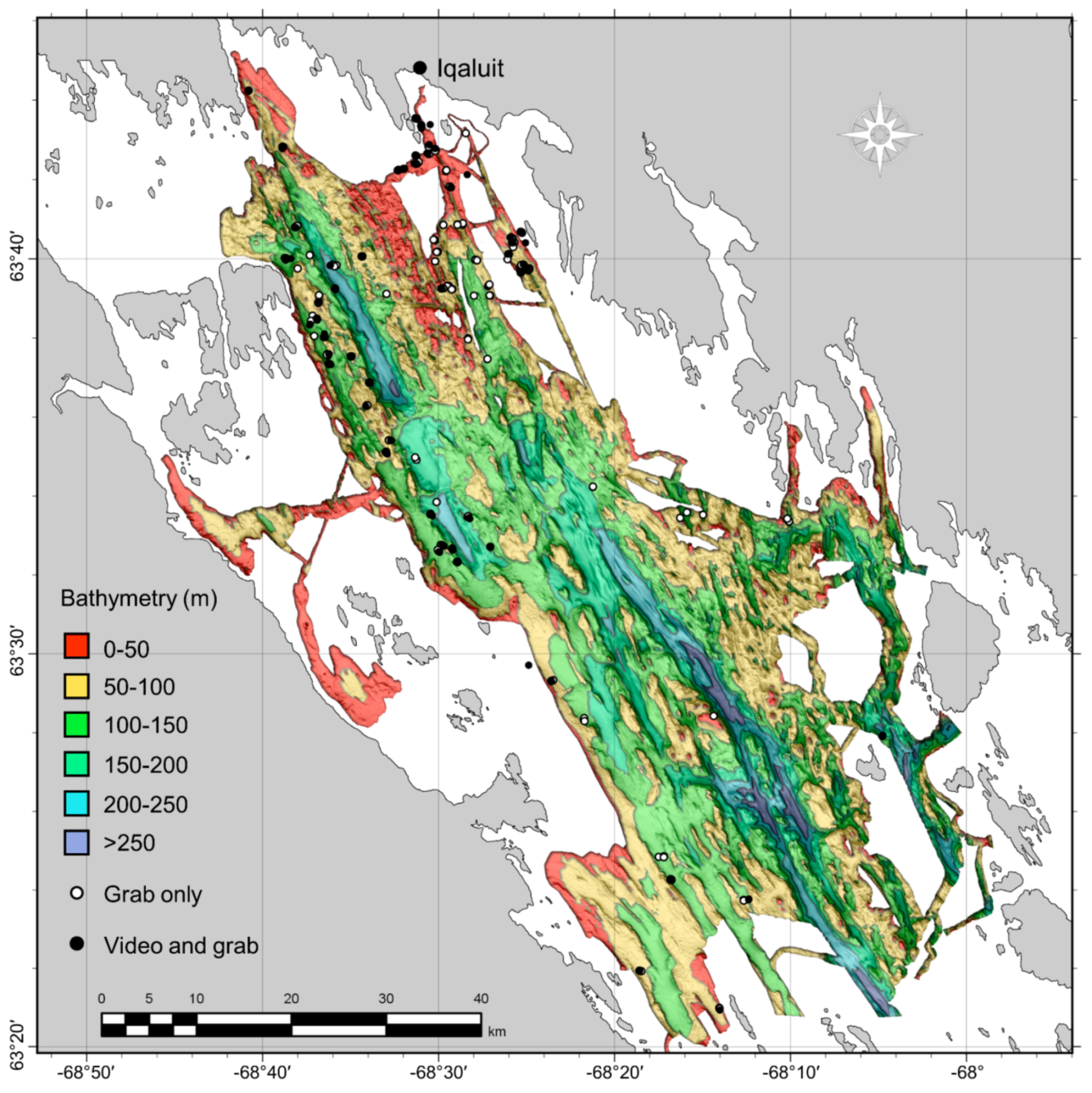
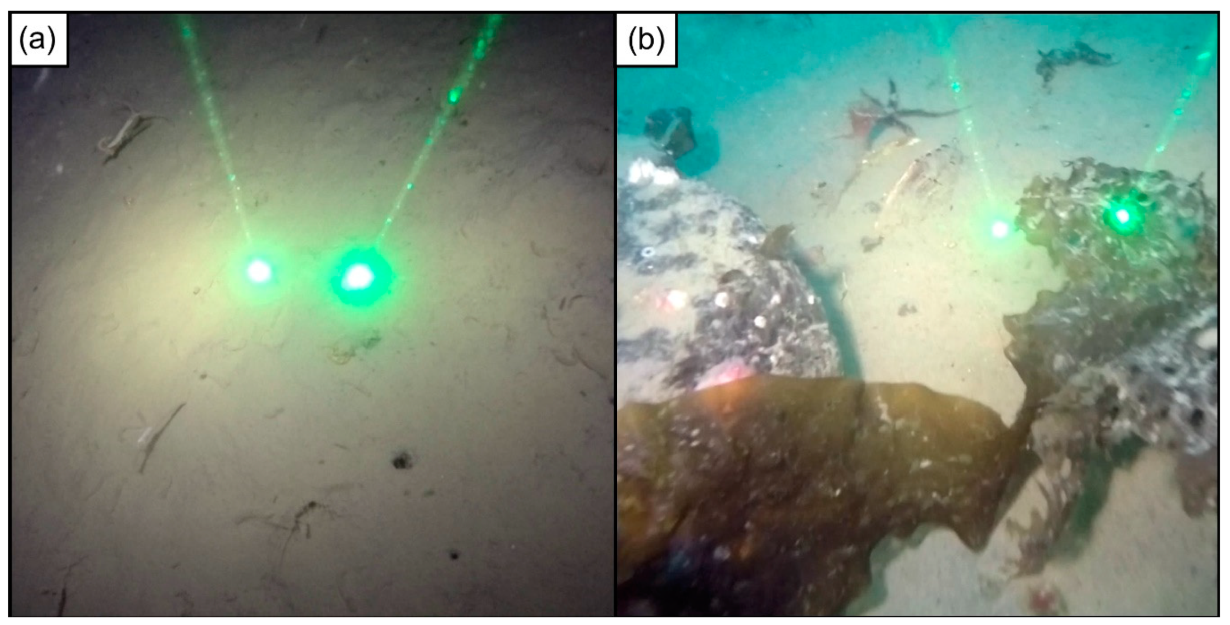
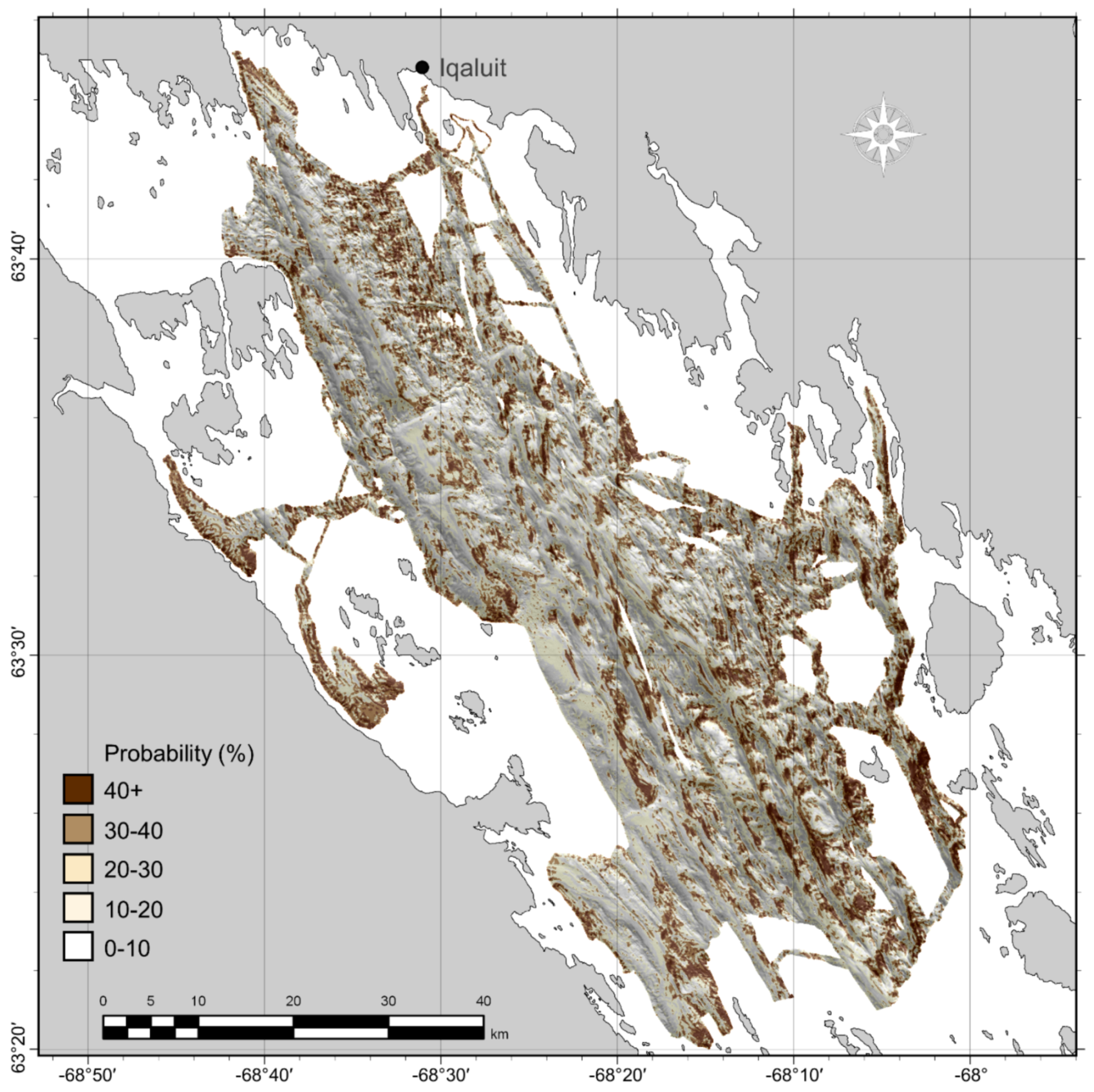
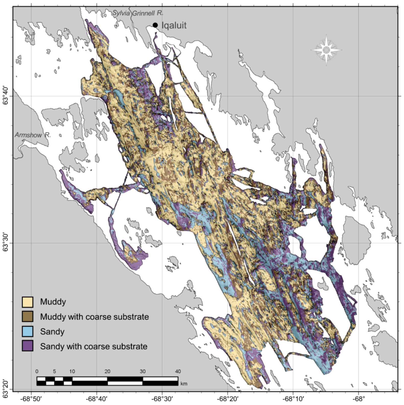
The predicted seabed sediment classes generally agreed with expectation given the geomorphology of the bay, yet particular locations without ground-truth data require further investigation. The majority of the low-relief seabed was classified as “muddy,” which is not surprising given what was observed in grab samples and underwater video (e.g., Figure 6 and Figure 7a). Sandy sediments predicted south and southwest of Iqaluit may be partially attributable to sediment input from the Sylvia Grinnell River, directly west of the city. This is also an area of distinct sea-ice scouring [
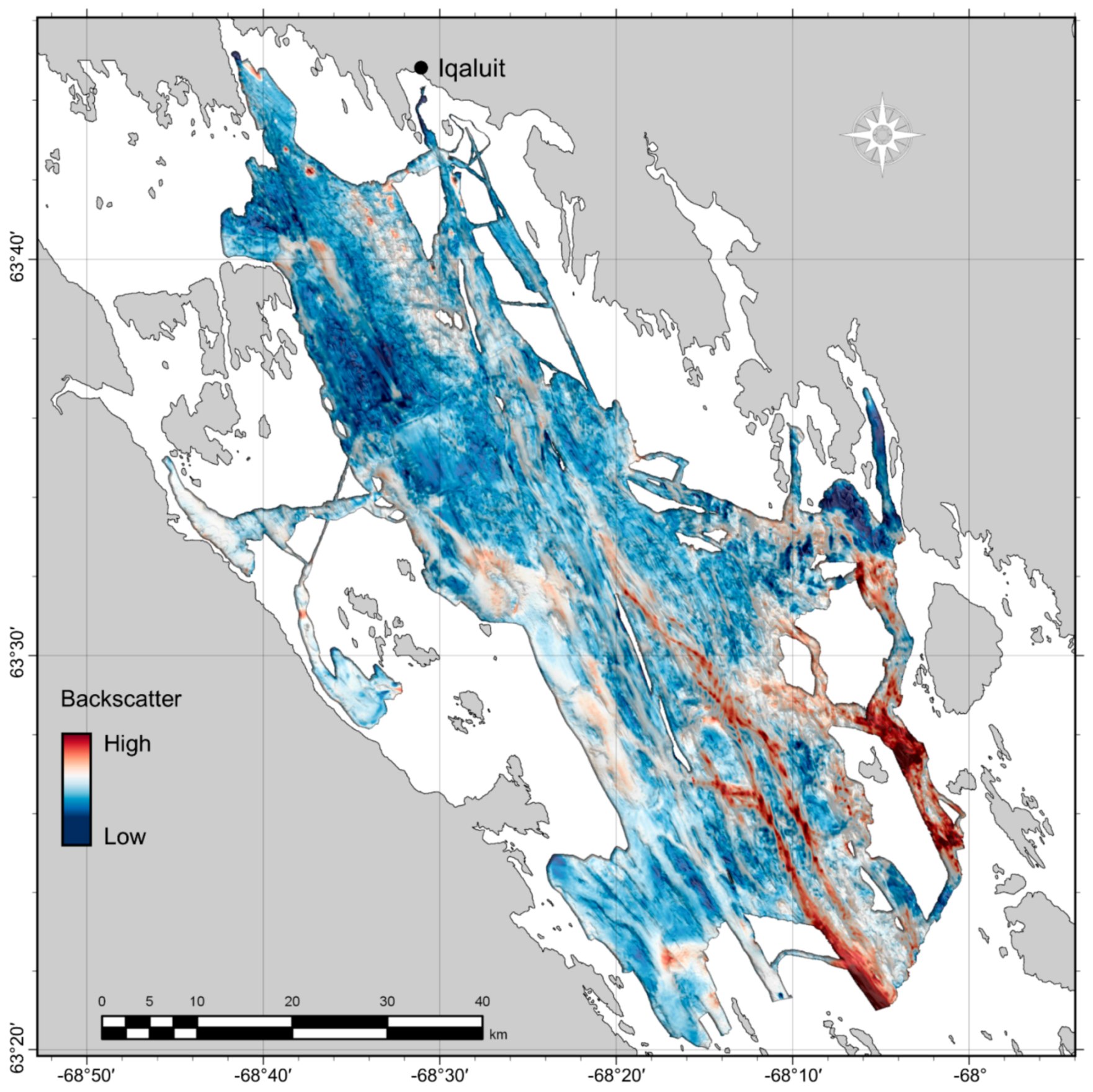
42] with higher acoustic backscatter than the surrounding seabed (Figure 5) and several distinctly reflective features that were classified as “sandy with coarse substrate.” This class was also predicted at several locations along the coast, fining to muddier grain sizes with increasing distance and depth. Otherwise, exposed coarse substrates predicted along the flanks of steep topographic features may be attributable to current winnowing of unstable fine sediments [
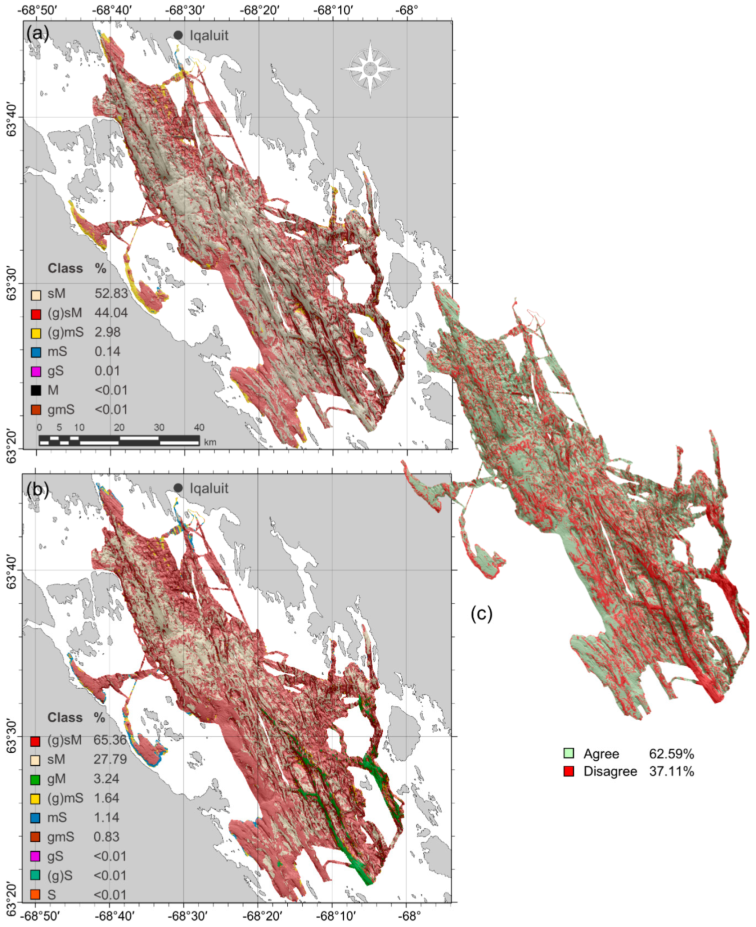
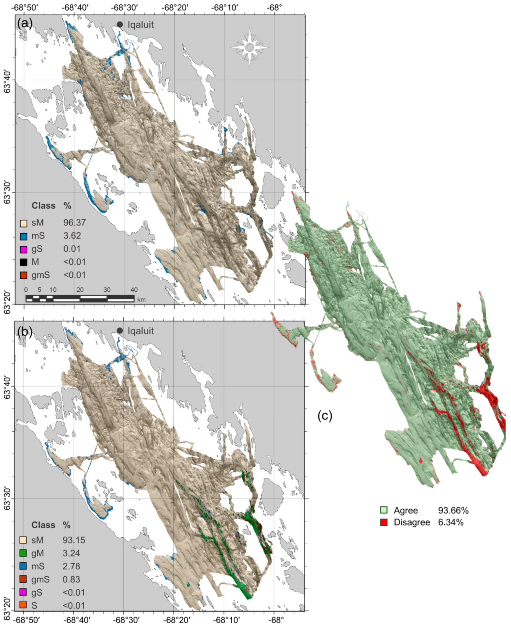
69]. This is likely the case in the high-relief, deep southeastern channels, where coarse substrates were predicted extensively. Further investigation is necessary in these deep channels though—this was an unsampled area of high disagreement between the categorical and quantitative models (Figure 8 and Figure 9). One might expect a muddier composition at the bottoms of these deep channels, yet sandier grain sizes were predicted, likely as a product of the high backscatter response (Figure 5).

4.1. Model Comparison

There was little difference in accuracy between quantitative and categorical Random Forest approaches when using spatially explicit cross-validation methods but their maps differed substantially. Using a two-class scheme, it was possible to tune the threshold of occurrence for the probabilistic output of the categorical model to obtain a higher accuracy than the quantitative model and this was selected for the final map. The most noticeable difference between maps was that the quantitative approach predicted extensive patches of sediment classes that were not observed in the ground-truth data, where the categorical approach predicted the most commonly observed classes. The predicted proportions and distributions of the classes also differed between approaches.
Although the quantitative Random Forest approach failed at extrapolation in this study, it has several characteristics that may be otherwise desirable. Because classification of quantitative predictions is done post hoc, this method might avoid some of the difficulty associated with predicting unbalanced classes—one of the major shortcomings of the categorical approach. Furthermore, as demonstrated here, predictions are not constrained to the classes that were sampled. Thus, if the model were fit well, it may be possible to predict rare and unsampled classes at new locations, while this is not feasible with the categorical approach. This may be a particularly useful quality if unsampled areas are expected to contain different sediment characteristics than the sample sites, yet it requires a high degree of confidence in the modelled relationships between grain size composition and the explanatory variables. The spatial leave-one-out CV error matrices for classified quantitative predictions (Appendix D) failed to indicate that the model could successfully predict rare classes in this study and we did not have the confidence to adopt predictions of unobserved classes in unsampled areas. It is quite possible that these areas do actually contain different sedimentary characteristics though, as their morphology and backscatter characteristics were unique but there is no way to confirm this. Sampling these areas would be a priority in future work.
It is also worth considering characteristics of the unclassified quantitative predictions of mud, sand, and gravel, which may offer some advantages over classification. These predictions represent gradational changes in sediment composition, which are more realistic and potentially more desirable than discrete classes. If classes are required, quantitative predictions are completely flexible with regards to classification scheme. Because the quantitative values remain the same, it is not necessary to run through the model fitting procedure to test different classifications – the class boundaries simply need to be adjusted. Other methods could also be used to optimize the classification of quantitative predictions to produce relevant and distinct classes, such as multivariate clustering. This way, it is possible to define an appropriate number of classes with boundaries that are most relevant to a given study area.
The qualities of the categorical Random Forest approach ultimately made it more suitable for this study but one major difficulty was assessing whether rare classes were predicted correctly. Because the data were spatially autocorrelated, samples of rare classes were likely to occur close to one another. Using a spatial CV approach, in which samples proximal to the test data are omitted from model training (as in S-LOO CV) or proximal samples are not allowed for either training or testing (as in SR-LOO CV), can potentially remove most or all other samples of a rare class, making it impossible to assess if it was predicted accurately. Selecting a classification scheme that matches the data facilitates the estimation of accuracy by ensuring an adequate number of samples for training and testing each class. Here, the Folk and simplified Folk schemes each contained several classes with very few observations (< 5) and the success in predicting these could not be confidently determined. The muddy/sandy classification better fit the data, providing adequate samples of each class to evaluate predictive success.
Though the muddy/sandy classification was a good fit given these data (Figure 6), the class prevalence was still unbalanced. Another solution afforded by the categorical approach is that the threshold of occurrence can be optimized. Setting this threshold to maximize the sum of sensitivity + specificity equally weights the success in predicting each class and this produced higher extrapolative (i.e., S-LOO CV) accuracy than the quantitative approach, especially after removing superfluous variables. Another common approach used to predict rare classes is to subsample the dataset to ensure equal class representation but that requires enough samples of the rarest class to allow a reasonable subsample size. Furthermore, some research has suggested that the proportions of classes in the training data should be representative of the actual proportions of these classes [36].

4.2. Spatial Assessment

Spatial autocorrelation inflated estimates of predictive accuracy regardless of the modelling approach or classification scheme for both grain size and coarse substrate models, hindering the ability to determine whether the models could successfully extrapolate grain size classes at unsampled locations. Similar to LOO CV, many common model validation techniques (e.g., sample partitioning, k-fold CV) have no spatial component. For this study, non-spatial techniques failed to correctly estimate the model’s ability to extrapolate. If LOO CV were used in isolation to evaluate the categorical simplified Folk predictions for example, the percent correctly classified and κ values (85.50%; 0.52) would suggest the model is highly accurate and reliable. In reality though, it fails to extrapolate beyond the sphere of spatial autocorrelation influence, with predictions no better than random.
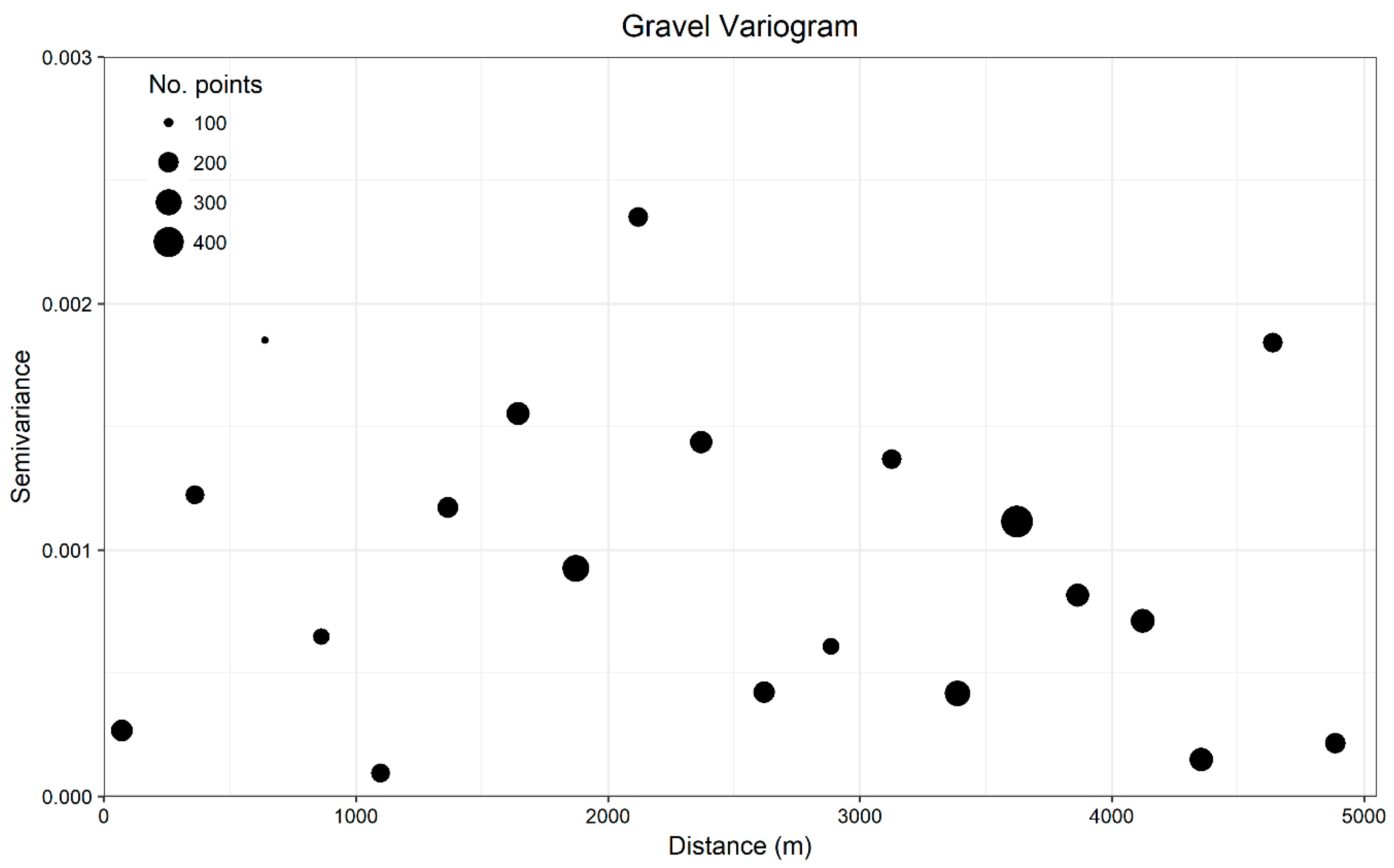
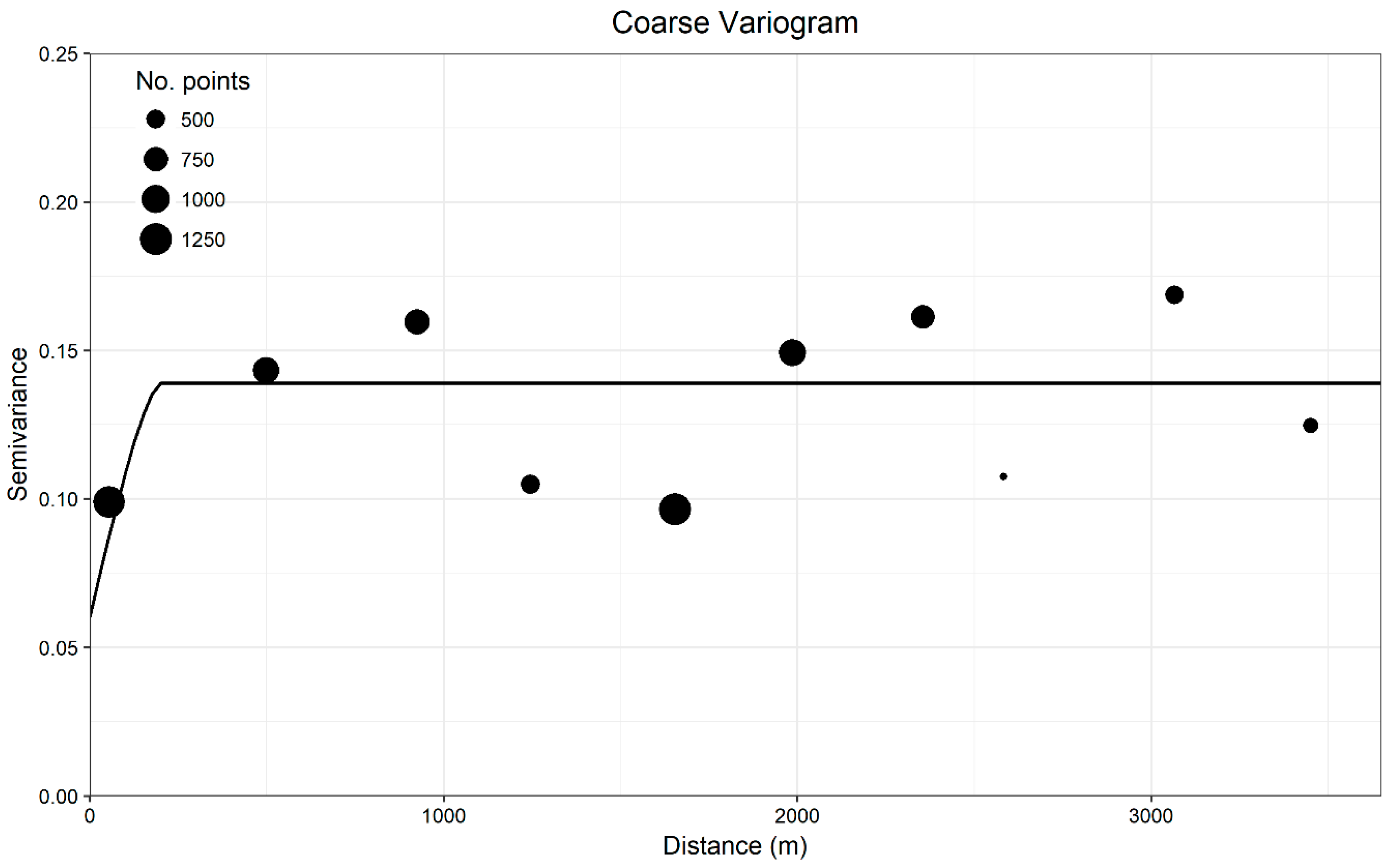
The SR-LOO CV for the coarse substrate model suggested not only that spatial autocorrelation inflated estimates of accuracy but also that Random Forest was spatially overfitting, hindering extrapolation. This is an important issue for severely autocorrelated datasets that is not necessarily solved by other spatial validation approaches that allow for proximal training samples such as S-LOO CV or spatial blocking. Though SR-LOO CV shows promise for reducing overfitting and providing non-biased estimates of accuracy, we note that the computational effort may not always be realistic. One hundred random samples of each spatially-buffered leave-one-out sample set (n = 324) yielded 32,400 sub-samples and corresponding Random Forest models for one SR-LOO CV run. Furthermore, the “embarrassingly parallel” qualities of Random Forest were leveraged to implement SR-LOO CV here, which is not characteristic of most other modelling methods. Simpler alternatives could involve aggregating sample transects to a single point and adjusting the raster resolution, yet this may be less attractive if a high resolution is desired. How such methods compare with the SR-LOO CV remains to be explored.

4.3. Spatial Prediction

It is important to distinguish between interpolating a well-sampled area and extrapolating to unsampled locations [67]. Though it is becoming standard practice to report predictive accuracy, it is less common to differentiate between these predictive spatial qualities, which are partly determined by sample distribution and intensity. Again, if interpolation is the goal, with somewhat uniform and well-distributed sampling, then standard non-spatial model evaluation methods may be appropriate (e.g., LOO CV, k-fold CV, partitioning). If samples are clustered, with parts of the study area unsampled, then it is necessary to evaluate for extrapolation, which may require a spatially explicit approach, as was the case here. This also may affect the appropriateness of categorical and quantitative approaches – if extrapolating to a potentially new sedimentary environment is the goal and if there is confidence in the modelled relationships between sediment and explanatory variables, then a quantitative approach may be useful for identifying unsampled or rare sediment classes. Here, we found that the flexibility of the threshold of occurrence using a categorical Random Forest approach resulted in superior extrapolative performance compared to a quantitative approach for a binary classification scheme. Given a set of classification requirements (e.g., regional compatibility) and a desire to maximize predictive accuracy of predetermined classes, it may be desirable to test both approaches where feasible – our results do not suggest the consistent superiority of one method over the other.
Recently there have been calls for greater transparency in reporting map quality, including uncertainty and error, to determine whether thematic maps are fit for purpose (e.g., [70,71]). This becomes especially important when providing maps as tools for management, where end-users may lack the technical understanding to critically evaluate a map [72]. The spatial component of distribution modelling is a potential source of data error [71] that is commonly neglected [52], yet which can be exacerbated due to marine sampling constraints. Here we have demonstrated the necessity of spatially explicit analysis for comparing the error and predictions between two seabed sediment mapping approaches and the potential pitfalls of neglecting to do so. Though many approaches have been tested and compared in the seabed mapping literature, these qualities are often ignored. The SR-LOO CV approach used here to model the presence of coarse substrates is similar to the variable scale selection procedure used by Holland et al. [68] but uses “embarrassingly parallel” Random Forests so that no samples are fully omitted. This is the first application of the approach in this context to our knowledge. Though the SR-LOO CV method was well-suited to modelling video transect data in this study, we acknowledge several other useful strategies [67] and tools [73] that are worth considering to address spatial sampling bias. Geostatistical methods may also be a preferable alternative for handling spatially dependent data depending on the modelling goals. The focus of this study was on modelling seabed sediments but the findings are relevant to other similar benthic distribution models including those of species and biotopes.

5. Conclusions

Neither categorical nor quantitative Random Forests performed consistently better between the classification schemes tested but the mapped predictions and the qualities of the models differed substantially, ultimately informing on the suitability of these methods. The ability of the quantitative approach to predict rare and unsampled classes may be an important quality depending on sample distribution and mapping goals, yet we found the probabilistic threshold qualities of the categorical approach with a binary scheme (i.e., “muddy/sandy”) made it more suitable for extrapolation in this study. Extrapolation was a necessary quality for these models because sample sites were clustered, with some areas not sampled.
There was evidence that the proximity of transect video observations caused both inflated estimates of accuracy and overfitting in the Random Forest models of coarse substrate. We conclude therefore that it should not be taken for granted that Random Forest will not overfit amidst autocorrelated data and spatially explicit methods may be necessary to ensure spatial independence, regardless of the modelling algorithm used. This is especially relevant for seabed mapping given the prevalence of transect data in this field.
From the results of this study we recommend that seabed map producers be specific about their predictive goals – especially whether the models are required to extrapolate to new environments and locations or whether they will “fill in the gaps” between sample sites (i.e., interpolate). This distinction can determine the appropriateness of modelling approaches and evaluation methods. We found it necessary to use spatially explicit strategies to evaluate whether the models in this study were able to extrapolate and that modelling highly autocorrelated data required both model fitting and testing in a spatially independent context.

Author Contributions

The authors of this paper contributed as follows: conceptualization, B.M. and M.D.; methodology, B.M. and M.D.; software, B.M.; validation, B.M.; formal analysis, B.M.; investigation, B.M. and A.A.; resources, E.E., A.A., T.B. and C.B.; data curation, B.M.; writing—original draft preparation, B.M.; writing—review and editing, M.D., C.B., T.B., A.A. and E.E.; visualization, B.M.; supervision, T.B. and E.E.; project administration, E.E. and T.B.; funding acquisition, E.E., T.B. and A.A.

Funding

This research was funded by ArcticNet as part of the project “Integrated Marine Geoscience to Guide Environmental Impact Assessment and Sustainable Development in Frobisher Bay, Nunavut.”

Acknowledgments

Thanks to the captain and crew of the RV Nuliajuk for assisting with data collection, to Drs. Alvin Simms and David Schneider for feedback on statistical methodology and to Kirsten Costello for assisting with data processing. Thanks to the community of Iqaluit and the Government of Nunavut Department of Environment Fisheries and Sealing Division for supporting this project.

Conflicts of Interest

The authors declare no conflict of interest. The funders had no role in the design of the study; in the collection, analyses or interpretation of data; in the writing of the manuscript or in the decision to publish the results.

Appendix A

Multibeam Echosounder Data Processing

Bathymetry data were imported to Qimera version 1.7; erroneous values were removed manually or using conservative spline filters. The data were corrected for tides using the Arctic9 tide model [74]. Data acquired in each survey year and system were processed separately, exported as a 10 m floating point geoTIFF grid and mosaicked in ESRI ArcGIS Pro v.2.1 to a single raster (Figure 4).
Uncalibrated MBES backscatter data from each survey year and system were processed using the Fledermaus Geocoder Toolbox (FMGT) and exported separately as floating point geoTIFF grid files. Focal statistics were used in ESRI ArcGIS Pro to smooth the data over a 5 x 5-cell neighborhood to reduce noise. The use of multisource backscatter datasets presents several difficulties as relative dB values partially depend on the acquisition parameters of individual MBES systems (e.g., operating frequency; [75]). If each survey has been adequately ground-truthed, disparate datasets can be analyzed separately and their results combined [76]. Here, some of the datasets had few or no ground truth samples. We therefore adopted a normalization approach by which separate datasets were harmonized using a “bulk shift” methodology [56,77]. This standardizes each survey using the most extensive as reference, operating under the assumption that relative backscatter strength is a function of substrate properties and is relatively stable throughout a given survey. All surveys were thus mosaicked to a single raster at 10 m resolution and a low pass filter was applied to smooth out remaining data noise (Figure 5).

Appendix B

Variable Scale Selection

For the quantitative models, we calculated Spearman’s correlation coefficient for each scale of each predictor variable with grain size composition (ALRsm and ALRgm) to test for non-parametric monotonic relationships. We attempted to determine up to two appropriate scales (i.e., “intrinsic scales”; [78]) for each predictor by identifying local peaks in the plot of correlation versus variable scale. Because calculating correlation coefficients between a multi-level categorical response (viz., grain size classes) and quantitative predictors is not as straightforward, we used univariate multinomial logistic regressions to test the ability of each predictor at each scale to explain the grain size sediment class. The residual deviance of the univariate models was plotted against variable scale and up to two local minima were identified in each graph as intrinsic scales. All correlation scores and multinomial logistic regressions were calculated in R using the cor() and multinom() functions within the “stats” and “nnet” packages [79,80].
We tested whether selected scales of a given variable were correlated with each other and removed the weakest variable (based on relationship with the response) if Spearman’s ρ ≥ 0.70 between predictors [60,61,62]. We then tested the correlation between all remaining scales of all variables and removed weaker variables in cases where Spearman’s ρ ≥ 0.70.

Appendix C

Variogram Analysis

Variograms were calculated for measurements of each grain size fraction and the presence of coarse sediments. The following model fits were obtained from the ArcGIS Geostatistical Wizard.
Figure A1. Mud fraction variogram circular model with 250 m lags; nugget = 0.0069, partial sill = 0.0162, major range = 1496.63 m.
Geosciences 09 00254 g0a1
Figure A2. Sand fraction variogram circular model with 250 m lags; nugget = 0.0050, partial sill = 0.0152, major range = 1210.05 m.
Geosciences 09 00254 g0a2
Figure A3. Gravel fraction variogram with 250 m lags.
Geosciences 09 00254 g0a3
Figure A4. Coarse substrate variogram circular model with 360 m lags; nugget = 0.0603, partial sill = 0.0786, major range = 199.12 m.
Geosciences 09 00254 g0a4

Appendix D

Error Matrices

Because the leave-one-out cross-validations (including spatial leave-one-out) produce a prediction for each sample point in the dataset, error matrices can be calculated between observed and predicted sediment classes for each sample. Note a slight difference in observed grain size classes caused by the complete absence of gravel from some samples. Quantitative samples were transformed to additive log-ratios, which do not allow zero values. The following tables (A1–A14) correspond to those discussed and compared in results Section 3.4 (“Grain Size Model Evaluation and Comparison”). Error matrices were also calculated to estimate the predictive performance of the categorical grain size and coarse substrate models after optimizing the threshold of occurrence to maximize the sum of sensitivity + specificity. Table A13 and Table A14 correspond to results Section 3.6 (“Combined Map and Model Tuning”).
Table A1. Categorical Folk LOO CV error matrix.
Observed
(g)mS(g)sMgmSgSMmSsM
Predicted(g)mS10400022
(g)sM943101029
gmS0000000
gS0002000
M0000000
mS1000042
sM530200339
Table A2. Categorical Folk S-LOO CV error matrix.
Observed
(g)mS(g)sMgmSgSMmSsM
Predicted(g)mS0102002
(g)sM1846000723
gmS0000000
gS0000000
M0000000
mS0100000
sM729301246
Table A3. Quantitative Folk LOO CV error matrix.
Observed
(g)mS(g)sMgmSgSmSsM
Predicted(g)mS430000
(g)sM165620437
gmS200200
gS000000
mS200020
sM11910018
Table A4. Quantitative Folk S-LOO CV error matrix.
Observed
(g)mS(g)sMgmSgSmSsM
Predicted(g)mS010200
(g)sM216630639
gmS100000
gS000000
mS000000
sM31100016
Table A5. Categorical simplified Folk LOO CV error matrix.
Observed
gmSgSMmSsM
PredictedgmS00000
gS02000
M00000
mS000187
sM30116142
Table A6. Categorical simplified Folk S-LOO CV error matrix.
Observed
gmSgSMmSsM
PredictedgmS00000
gS00000
M00000
mS02012
sM30133147
Table A7. Quantitative simplified Folk LOO CV error matrix.
Observed
gmSgSmSsM
PredictedgmS0220
gS0000
mS0083
sM3021130
Table A8. Quantitative simplified Folk S-LOO CV error matrix.
Observed
gmSgSmSsM
PredictedgmS0010
gS0000
mS0201
sM3030132
Table A9. Categorical muddy/sandy LOO CV error matrix.
Predicted Observed
MuddySandy
Muddy14219
Sandy820
Table A10. Categorical muddy/sandy S-LOO CV error matrix.
Predicted Observed
MuddySandy
Muddy14536
Sandy53
Table A11. Quantitative muddy/sandy LOO CV error matrix.
Predicted Observed
MuddySandy
Muddy13124
Sandy212
Table A12. Quantitative muddy/sandy S-LOO CV error matrix.
Predicted Observed
MuddySandy
Muddy13233
Sandy13
Table A13. Categorical muddy/sandy S-LOO CV error matrix with threshold of occurrence set to 0.18.
Observed
Predicted PresentAbsent
Present3047
Absent9103
Table A14. Coarse substrate SR-LOO CV error matrix with threshold of occurrence set to 0.27.
Observed
Predicted PresentAbsent
Present4457
Absent15176

Appendix E

Continuous Quantitative Model Performance

The predictive performance of continuous quantitative model predictions was estimated using:
1. Pearson’s and Spearman’s coefficients to determine the strength of linear and non-linear correlation between predicted the observed values;
2. mean absolute error (MAE) to determine, on average, the error in predicted percentages of mud, sand and gravel; and
3. the percent variance explained (%VE), to quantify the accuracy of the model standardized to the variance of the observed grain size fraction values.
Nearly all continuous quantitative predictions of sediment grain size seemed accurate using leave-one-out cross-validation (LOO CV) yet were less accurate using spatial (buffered) leave-one-out cross-validation S-LOO CV (Table A15). The LOO CV %VE suggested that the relative error of these predictions was less than the variance in the observed values but S-LOO CV %VE values were lower and negative, indicating a high amount of error relative to the measurements of each size class. Similarly, the non-relative error between predicted and observed values (i.e., the MAE) was higher in S-LOO CV predictions than LOO. With the exception of gravel predictions, all Pearson and Spearman correlation scores were lower in S-LOO predictions than LOO C
Table A15. Accuracies of unclassified quantitative grain size predictions using spatial and non-spatial cross-validations.
LOO CVS-LOO CV (1500 m)
Mud%VE60.96−6.42
MAE (%)8.2813.51
Pearson0.780.13
Spearman0.680.06
Sand%VE60.05−10.99
MAE (%)8.0112.91
Pearson0.780.06
Spearman0.670.03
Gravel%VE29.66−2.06
MAE (%)1.131.58
Pearson0.610.13
Spearman0.400.32

References

  1. Halpern, B.S.; Walbridge, S.; Selkoe, K.A.; Kappel, C.V.; Micheli, F.; D’Agrosa, C.; Bruno, J.F.; Casey, K.S.; Ebert, C.; Fox, H.E.; et al. A global map of human impact on marine ecosystems. Science 2008, 319, 948–952. [Google Scholar] [CrossRef] [PubMed]
  2. Costanza, R.; d’Arge, R.; de Groot, R.; Farber, S.; Grasso, M.; Hannon, B.; Limburg, K.; Naeem, S.; O’Neill, R.V.; Paruelo, J.; et al. The value of the world’s ecosystem services and natural capital. Nature 1997, 387, 253–260. [Google Scholar] [CrossRef]
  3. Ghermandi, A.; Nunes, P.A.L.D.; Portela, R.; Nalini, R.; Teelucksingh, S.S. Recreational, Cultural and Aesthetic Services from Estuarine and Coastal Ecosystems; FEEM Working Paper No. 121.2009; Fondazione Eni Enrico Mattei: Milan, Italy, 2010. [Google Scholar]
  4. Galparsoro, I.; Borja, A.; Uyarra, M.C. Mapping ecosystem services provided by benthic habitats in the European North Atlantic Ocean. Front. Mar. Sci. 2014, 1, 23. [Google Scholar] [CrossRef]
  5. Baker, E.K.; Harris, P.T. Habitat mapping and marine management. In Seafloor Geomorphology as Benthic Habitat: Geohab Atlas of Seafloor Geomorphic Features and Benthic Habitats; Harris, P.T., Baker, E.K., Eds.; Elsevier: Amsterdam, The Netherlands, 2012; pp. 23–38. [Google Scholar]
  6. Ehler, C.; Douvere, F. Marine Spatial Planning: A Step-by-Step Approach toward Ecosystem-Based Management; Intergovernmental Oceanographic Commission and Man and the Biosphere Programme; UNESCO: Paris, France, 2009. [Google Scholar]
  7. McArthur, M.A.; Brooke, B.P.; Przeslawski, R.; Ryan, D.A.; Lucieer, V.L.; Nichol, S.; McCallum, A.W.; Mellin, C.; Cresswell, I.D.; Radke, L.C. On the use of abiotic surrogates to describe marine benthic biodiversity. Estuar. Coast. Shelf Sci. 2010, 88, 21–32. [Google Scholar] [CrossRef]
  8. Beaman, R.J.; Daniell, J.J.; Harris, P.T. Geology-benthos relationships on a temperate rocky bank, eastern Bass Strait, Australia. Mar. Freshw. Res. 2005, 56, 943–958. [Google Scholar] [CrossRef]
  9. Diesing, M.; Green, S.L.; Stephens, D.; Lark, R.M.; Stewart, H.A.; Dove, D. Mapping seabed sediments: Comparison of manual, geostatistical, object-based image analysis and machine learning approaches. Cont. Shelf Res. 2014, 84, 107–119. [Google Scholar] [CrossRef] [Green Version]
  10. Stephens, D.; Diesing, M. A comparison of supervised classification methods for the prediction of substrate type using acoustic and legacy grain-size data. PLoS ONE 2014, 9, e93950. [Google Scholar] [CrossRef]
  11. Che Hasan, R.; Ierodiaconou, D.; Monk, J. Evaluation of four supervised learning methods for benthic habitat mapping using backscatter from multi-beam sonar. Remote Sens. 2012, 4, 3427–3443. [Google Scholar] [CrossRef]
  12. Todd, B.J.; Fader, G.B.J.; Courtney, R.C.; Pickrill, R.A. Quaternary geology and surficial sediment processes, Browns Bank, Scotian Shelf, based on multibeam bathymetry. Mar. Geol. 1999, 162, 165–214. [Google Scholar] [CrossRef]
  13. Brown, C.J.; Smith, S.J.; Lawton, P.; Anderson, J.T. Benthic habitat mapping: A review of progress towards improved understanding of the spatial ecology of the seafloor using acoustic techniques. Estuar. Coast. Shelf Sci. 2011, 92, 502–520. [Google Scholar] [CrossRef]
  14. Galparsoro, I.; Agrafojo, X.; Roche, M.; Degrendele, K. Comparison of supervised and unsupervised automatic classification methods for sediment types mapping using multibeam echosounder and grab sampling. Ital. J. Geosci. 2015, 134, 41–49. [Google Scholar] [CrossRef] [Green Version]
  15. Diesing, M.; Kröger, S.; Parker, R.; Jenkins, C.; Mason, C.; Weston, K. Predicting the standing stock of organic carbon in surface sediments of the North–West European continental shelf. Biogeochemistry 2017, 135, 183–200. [Google Scholar] [CrossRef]
  16. Siwabessy, P.J.W.; Tran, M.; Picard, K.; Brooke, B.P.; Huang, Z.; Smit, N.; Williams, D.K.; Nicholas, W.A.; Nichol, S.L.; Atkinson, I. Modelling the distribution of hard seabed using calibrated multibeam acoustic backscatter data in a tropical, macrotidal embayment: Darwin Harbour, Australia. Mar. Geophys. Res. 2018, 39, 249–269. [Google Scholar] [CrossRef]
  17. Li, J.; Tran, M.; Siwabessy, J. Selecting optimal random Forest predictive models: A case study on predicting the spatial distribution of seabed hardness. PLoS ONE 2016, 11, e0149089. [Google Scholar] [CrossRef] [PubMed]
  18. Li, J.; Potter, A.; Huang, Z.; Daniell, J.J.; Heap, A.D. Predicting Seabed Mud Content across the Australian Margin: Comparison of Statistical and Mathematical Techniques Using a Simulation Experiment; Geoscience Australia: Canberra, Australia, 2010. [Google Scholar]
  19. Ierodiaconou, D.; Monk, J.; Rattray, A.; Laurenson, L.; Versace, V.L. Comparison of automated classification techniques for predicting benthic biological communities using hydroacoustics and video observations. Cont. Shelf Res. 2011, 31, S28–S38. [Google Scholar] [CrossRef]
  20. Folk, R.L. The distinction between grain size and mineral composition in sedimentary-rock nomenclature. J. Geol. 1954, 62, 344–359. [Google Scholar] [CrossRef]
  21. Long, D. BGS Detailed Explanation of Seabed Sediment Modified Folk Classification; British Geological Survey: Nottingham, UK, 2006. [Google Scholar]
  22. Connor, D.W.; Gilliland, P.M.; Golding, N.; Robinson, P.; Todd, D.; Verling, E. UKSeaMap: The Mapping of Seabed and Water Column Features of UK Seas; Joint Nature Conservation Committee: Peterborough, UK, 2006. [Google Scholar]
  23. European Environment Agency. EUNIS Habitat Classification; European Environment Agency: Copenhagen, Denmark, 2006. [Google Scholar]
  24. Davies, C.E.; Moss, D.; Hill, M.O. EUNIS Habitat Classification Revised; European Environment Agency: Copenhagen, Denmark, 2004. [Google Scholar]
  25. Strong, J.A.; Clements, A.; Lillis, H.; Galparsoro, I.; Bildstein, T.; Pesch, R. A review of the influence of marine habitat classification schemes on mapping studies: Inherent assumptions, influence on end products and suggestions for future developments. ICES J. Mar. Sci. 2018, 76, 10–22. [Google Scholar] [CrossRef]
  26. Stephens, D.; Diesing, M. Towards quantitative spatial models of seabed sediment composition. PLoS ONE 2015, 10, e0142502. [Google Scholar] [CrossRef]
  27. Diesing, M.; Stephens, D. A multi-model ensemble approach to seabed mapping. J. Sea Res. 2015, 100, 62–69. [Google Scholar] [CrossRef]
  28. Elith, J.; Graham, C.H.; Anderson, R.P.; Dudík, M.; Ferrier, S.; Guisan, A.; Hijmans, R.J.; Huettmann, F.; Leathwick, J.R.; Lehmann, A.; et al. Novel methods improve prediction of species’ distributions from occurrence data. Ecography 2006, 29, 129–151. [Google Scholar] [CrossRef]
  29. Hernandez, P.A.; Graham, C.H.; Master, L.L.; Albert, D.L. The effect of sample size and species characteristics on performance of different species distribution modeling methods. Ecography 2006, 29, 773–785. [Google Scholar] [CrossRef]
  30. Olden, J.D.; Lawler, J.J.; Poff, N.L. Machine learning methods without tears: A primer for ecologists. Q. Rev. Biol. 2008, 83, 171–193. [Google Scholar] [CrossRef] [PubMed]
  31. Li, J.; Alvarez, B.; Siwabessy, J.; Tran, M.; Huang, Z.; Przeslawski, R.; Radke, L.; Howard, F.; Nichol, S. Application of random forest, generalised linear model and their hybrid methods with geostatistical techniques to count data: Predicting sponge species richness. Environ. Model. Softw. 2017, 97, 112–129. [Google Scholar] [CrossRef]
  32. Breiman, L. Random forests. Mach. Learn. 2001, 45, 5–32. [Google Scholar] [CrossRef]
  33. Aitchison, J. The statistical analysis of compositional data. J. R. Stat. Soc. 1982, 44, 139–177. [Google Scholar] [CrossRef]
  34. Araújo, M.B.; Guisan, A. Five (or so) challenges for species distribution modelling. J. Biogeogr. 2006, 33, 1677–1688. [Google Scholar] [CrossRef]
  35. Hirzel, A.; Guisan, A. Which is the optimal sampling strategy for habitat suitability modelling. Ecol. Model. 2002, 157, 331–341. [Google Scholar] [CrossRef]
  36. Millard, K.; Richardson, M. On the importance of training data sample selection in random forest image classification: A case study in peatland ecosystem mapping. Remote Sens. 2015, 7, 8489–8515. [Google Scholar] [CrossRef]
  37. Hammond, T.O.; Verbyla, D.L. Optimistic bias in classification accuracy assessment. Int. J. Remote Sens. 1996, 17, 1261–1266. [Google Scholar] [CrossRef]
  38. Legendre, P. Spatial autocorrelation: Trouble or new paradigm? Ecology 1993, 74, 1659–1673. [Google Scholar] [CrossRef]
  39. Segurado, P.; Araújo, M.B.; Kunin, W.E. Consequences of spatial autocorrelation for niche-based models. J. Appl. Ecol. 2006, 43, 433–444. [Google Scholar] [CrossRef]
  40. Hodgson, D.A. Quaternary Geology of Western Meta Incognita Peninsula and Iqaluit area, Baffin Island, Nunavut; Bulletin 582; Geological Survey of Canada: Ottawa, ON, Canada, 2005. [Google Scholar]
  41. Tremblay, T.; Day, S.; McNeil, R.; Smith, K.; Richardson, M.; Shirley, J. Overview of Surficial Geology Mapping and Geochemistry in the Sylvia Grinnell Lake Area, Baffin Island, Nunavut; Summary of Activities 2015; Canada-Nunavut Geoscience Office: Iqaluit, Canada, 2015; pp. 107–120.
  42. Deering, R.; Misiuk, B.; Bell, T.; Forbes, D.L.; Edinger, E.; Tremblay, T.; Telka, A.; Aitken, A.; Campbell, C. Characterization of the Seabed and Postglacial Sediments of Inner Frobisher Bay, Baffin Island, Nunavut; Summary of Activities 2018; Canada-Nunavut Geoscience Office: Iqaluit, Canada, 2018; pp. 139–152.
  43. Weatherall, P.; Marks, K.M.; Jakobsson, M.; Schmitt, T.; Tani, S.; Arndt, J.E.; Rovere, M.; Chayes, D.; Ferrini, V.; Wigley, R. A new digital bathymetric model of the world’s oceans. Earth Space Sci. 2015, 2, 331–345. [Google Scholar] [CrossRef]
  44. ESRI. World Light Gray Canvas [Basemap]. 2011. Available online: https://www.arcgis.com/home/item.html?id=ed712cb1db3e4bae9e85329040fb9a49 (accessed on 29 March 2019).
  45. Eleftheriou, A.; Moore, D.C. Macrofauna techniques. In Methods for the Study of Marine Benthos; Eleftheriou, A., Ed.; Wiley-Blackwell: Chichester, UK, 2013; pp. 175–251. [Google Scholar]
  46. Rees, H.L. (Ed.) Guidelines for the Study of the Epibenthos of Subtidal Environments; ICES Techniques in Marine Environmental Sciences; International Council for the Exploration of the Sea: Copenhagen, Denmark, 2009. [Google Scholar]
  47. Whitmire, C.E.; Embley, R.W.; Wakefield, W.W.; Merle, S.G.; Tissot, B.N. A quantitative approach for using multibeam sonar data to map benthic habitats. In Mapping the Seafloor for Habitat Characterization: Geological Association of Canada, Special Paper 47; Geological Association of Canada: St. John’s, NL, Canada, 2007; pp. 111–126. [Google Scholar]
  48. Breiman, L. Bagging predictors. Mach. Learn. 1996, 24, 123–140. [Google Scholar] [CrossRef] [Green Version]
  49. Cutler, D.R.; Edwards, T.C.; Beard, K.H.; Cutler, A.; Hess, K.T.; Gibson, J.; Lawler, J.J. Random Forests for classification in ecology. Ecology 2007, 88, 2783–2792. [Google Scholar] [CrossRef] [PubMed]
  50. Liaw, A.; Wiener, M. Classification and regression by randomForest. R News 2002, 2, 18–22. [Google Scholar]
  51. Heikkinen, R.K.; Marmion, M.; Luoto, M. Does the interpolation accuracy of species distribution models come at the expense of transferability? Ecography 2012, 35, 276–288. [Google Scholar] [CrossRef]
  52. Bell, D.M.; Schlaepfer, D.R. On the dangers of model complexity without ecological justification in species distribution modeling. Ecol. Model. 2016, 330, 50–59. [Google Scholar] [CrossRef] [Green Version]
  53. Pawlowsky-Glahn, V.; Olea, R.A. Geostatistical Analysis of Compositional Data; Studies in Mathematical Geology; Oxford University Press: New York, NY, USA, 2004. [Google Scholar]
  54. Diesing, M. Quantitative Spatial Prediction of Seabed Sediment Composition; Centre for Environment Fisheries and Aquaculture: Suffolk, UK, 2015.
  55. Liu, C.; Berry, P.M.; Dawson, T.P.; Pearson, R.G. Selecting thresholds of occurrence in the prediction of species distributions. Ecography 2005, 28, 385–393. [Google Scholar] [CrossRef]
  56. Misiuk, B.; Lecours, V.; Bell, T. A multiscale approach to mapping seabed sediments. PLoS ONE 2018, 13, e0193647. [Google Scholar] [CrossRef]
  57. Lecours, V.; Devillers, R.; Simms, A.E.; Lucieer, V.L.; Brown, C.J. Towards a framework for terrain attribute selection in environmental studies. Environ. Model. Softw. 2017, 89, 19–30. [Google Scholar] [CrossRef]
  58. Lecours, V. Terrain Attribute Selection for Spatial Ecology (TASSE). Version 1.0. 2015. Available online: https://doi.org/10.13140/RG.2.2.35147.18728 (accessed on 29 March 2019).
  59. Walbridge, S.; Slocum, N.; Pobuda, M.; Wright, D.J. Unified geomorphological analysis workflows with Benthic Terrain Modeler. Geosciences 2018, 8, 94. [Google Scholar] [CrossRef]
  60. Downie, A.-L.; Dove, D.; Westhead, K.; Diesing, M.; Green, S.L.; Cooper, R. Semi-Automated Mapping of Rock in the North Sea; JNCC: Peterborough, UK, 2016. [Google Scholar]
  61. Gottschalk, T.K.; Aue, B.; Hotes, S.; Ekschmitt, K. Influence of grain size on species–habitat models. Ecol. Model. 2011, 222, 3403–3412. [Google Scholar] [CrossRef]
  62. Dormann, C.F.; Elith, J.; Bacher, S.; Buchmann, C.; Carl, G.; Carré, G.; Marquéz, J.R.G.; Gruber, B.; Lafourcade, B.; Leitão, P.J.; et al. Collinearity: A review of methods to deal with it and a simulation study evaluating their performance. Ecography 2013, 36, 27–46. [Google Scholar] [CrossRef]
  63. Cohen, J. A coefficient of agreement for nominal scales. Educ. Psychol. Meas. 1960, 20, 37–46. [Google Scholar] [CrossRef]
  64. Fielding, A.H.; Bell, J.F. A review of methods for the assessment of prediction errors in conservation presence/absence models. Environ. Conserv. 1997, 24, 38–49. [Google Scholar] [CrossRef]
  65. Bahn, V.; McGill, B.J. Testing the predictive performance of distribution models. Oikos 2013, 122, 321–331. [Google Scholar] [CrossRef]
  66. Le Rest, K.; Pinaud, D.; Monestiez, P.; Chadoeuf, J.; Bretagnolle, V. Spatial leave-one-out cross-validation for variable selection in the presence of spatial autocorrelation. Glob. Ecol. Biogeogr. 2014, 23, 811–820. [Google Scholar] [CrossRef] [Green Version]
  67. Roberts, D.R.; Bahn, V.; Ciuti, S.; Boyce, M.S.; Elith, J.; Guillera-Arroita, G.; Hauenstein, S.; Lahoz-Monfort, J.J.; Schröder, B.; Thuiller, W.; et al. Cross-validation strategies for data with temporal, spatial, hierarchical or phylogenetic structure. Ecography 2017, 40, 913–929. [Google Scholar] [CrossRef]
  68. Holland, J.D.; Bert, D.G.; Fahrig, L. Determining the spatial scale of species’ response to habitat. BioScience 2004, 54, 227–233. [Google Scholar] [CrossRef]
  69. Syvitski, J.P.M. On the deposition of sediment within glacier-influenced fjords: Oceanographic controls. Mar. Geol. 1989, 85, 301–329. [Google Scholar] [CrossRef]
  70. Mitchell, P.J.; Downie, A.-L.; Diesing, M. How good is my map? A tool for semi-automated thematic mapping and spatially explicit confidence assessment. Environ. Model. Softw. 2018, 108, 111–122. [Google Scholar] [CrossRef]
  71. Barry, S.; Elith, J. Error and uncertainty in habitat models. J. Appl. Ecol. 2006, 43, 413–423. [Google Scholar] [CrossRef]
  72. Lecours, V. On the use of maps and models in conservation and resource management (warning: Results may vary). Front. Mar. Sci. 2017, 4, 288. [Google Scholar] [CrossRef]
  73. Valavi, R.; Elith, J.; Lahoz-Monfort, J.J.; Guillera-Arroita, G. BLOCKCV: An R package for generating spatially or environmentally separated folds for k-fold cross-validation of species distribution models. Methods Ecol. Evol. 2018, 10, 225–232. [Google Scholar] [CrossRef]
  74. Collins, A.K.; Hannah, C.G.; Greenberg, D. Validation of a High Resolution Modelling System for Tides in the Canadian Arctic Archipelago; Bedford Institute of Oceanography: Dartmouth, NS, Canada, 2011. [Google Scholar]
  75. Lurton, X.; Lamarche, G. Backscatter Measurements by Seafloor-Mapping Sonars. Guidelines and Recommendations, reported by GeoHab Backscatter Working Group. 2015. Available online: http://geohab.org/wp-content/uploads/2013/02/BWSG-REPORT-MAY2015.pdf (accessed on 31 March 2019).
  76. Lacharité, M.; Brown, C.J.; Gazzola, V. Multisource multibeam backscatter data: Developing a strategy for the production of benthic habitat maps using semi-automated seafloor classification methods. Mar. Geophys. Res. 2018, 39, 307–322. [Google Scholar] [CrossRef]
  77. Hughes Clarke, J.E.; Iwanowska, K.K.; Parrott, R.; Duffy, G.; Lamplugh, M.; Griffin, J. Inter-calibrating multi-source, multi-platform backscatter data sets to assist in compiling regional sediment type maps: Bay of Fundy. In Proceedings of the Canadian Hydrographic Conference and National Surveyors Conference 2008, Victoria, BC, Canada, 8 May 2008; Volume 8–2, p. 22. [Google Scholar]
  78. Lechner, A.M.; Langford, W.T.; Jones, S.D.; Bekessy, S.A.; Gordon, A. Investigating species–environment relationships at multiple scales: Differentiating between intrinsic scale and the modifiable areal unit problem. Ecol. Complex. 2012, 11, 91–102. [Google Scholar] [CrossRef]
  79. R Core Team. R: A Language and Environment for Statistical Computing; R Foundation for Statistical Computing: Vienna, Austria, 2018. [Google Scholar]
  80. Venables, W.N.; Ripley, B.D. Modern Applied Statistics with S, 4th ed.; Springer: New York, NY, USA, 2002. [Google Scholar]
Figure 1. Ternary diagrams with (a) Folk, (b) simplified Folk and (c) European nature information system (EUNIS) classes.
Geosciences 09 00254 g001
Figure 2. Two common supervised workflows for producing objective classified seabed sediment maps.
Geosciences 09 00254 g002
Figure 3. (a) Frobisher Bay, Nunavut, Canada with 200 m bathymetric contours from the GEBCO_2014 grid (The General Bathymetric Chart of the Oceans; [43]) and coastline reproduced from ESRI [44], with (b) location on southeastern Baffin Island and (c) the study area – inner Frobisher Bay.
Geosciences 09 00254 g003
Figure 4. Inner Frobisher Bay multibeam echosounder (MBES) bathymetry contoured at 50 m with shaded terrain and sample sites.
Geosciences 09 00254 g004
Figure 5. Inner Frobisher Bay relative MBES backscatter.
Geosciences 09 00254 g005
Figure 6. Grain size composition of sediment samples with class membership for the three schemes.
Geosciences 09 00254 g006
Figure 7. Examples of coarse sediment (a) absence and (b) presence in underwater video.
Geosciences 09 00254 g007
Figure 8. Predicted Folk grain size classes for (a) categorical and (b) quantitative models, with (c) agreement between predictions.
Geosciences 09 00254 g008
Figure 9. Predicted simplified Folk grain size classes for (a) categorical and (b) quantitative models, with (c) agreement between predictions.
Geosciences 09 00254 g009
Figure 10. Predicted “muddy/sandy” grain size classes for (a) categorical and (b) quantitative Random Forest models, with (c) agreement between predictions.
Geosciences 09 00254 g010
Figure 11. Predicted probability of coarse substrates using the spatially resampled leave-one-out cross validation (SR-LOO CV) (200 m) model.
Geosciences 09 00254 g011
Figure 12. Combined map of grain size classification and coarse substrate predictions.
Geosciences 09 00254 g012
Table 1. Coarse substrate observations from underwater video frames.
Coarse SubstratesRaster Cells
Present65
Absent259
Table 2. Scale-specific variables selected for sediment grain size models.
ALRsmALRgmClassification
VariableSpatial Scale (m)VariableSpatial Scale (m)VariableSpatial Scale (m)
Backscatter-Bathymetry-Bathymetry-
Bathymetry-Backscatter-Backscatter-
Distance from coast-Distance from coast-Distance from coast-
Backscatter range200Backscatter SD100Backscatter range250
Eastness50Eastness100Backscatter SD100
Eastness500Eastness400Eastness10
Northness10Northness250Eastness450
Plan curvature50Plan curvature50Northness10
Plan curvature350Plan curvature300Plan curvature150
Profile curvature450Profile curvature300Plan curvature300
RDMV300Profile curvature450Profile curvature300
SA:PA10Slope10RDMV200
Slope10Slope450RDMV350
Slope500VRM 200Slope10
VRM400VRM 400Slope450
VRM 10
Table 3. Variables selected for coarse substrate model.
Coarse Substrates
VariableScale (m)
Bathymetry-
Backscatter-
Distance from coast-
Backscatter SD100
Eastness100
Eastness500
Northness250
Plan curvature 100
Plan curvature 350
Profile curvature10
RDMV100
RDMV300
Slope200
VRM100
VRM350
Table 4. Performance of quantitative and categorical grain size predictions using three schemes with spatial and non-spatial cross-validations.
LOO CVS-LOO CV (1500 m)
CategoricalQuantitativeCategoricalQuantitative
Folk% correctly classified54.6448.4646.7248.58
Kappa0.250.140.120.10
Simplified Folk% correctly classified85.5082.2578.7978.11
Kappa0.520.340.050.04
Muddy/Sandy% correctly classified86.2984.6278.3679.88
Kappa0.530.410.060.11
Table 5. Threshold-independent accuracy of coarse substrate model using spatial and non-spatial cross validation (CV) approaches and with spatially independent training data.
LOO CVS-LOO CV (200 m)SR-LOO CV (200 m)
AUC0.860.670.76
Max kappa0.620.240.40
Table 6. Accuracies of grain size and coarse substrate components of combined seabed sediment predictions.
Muddy/Sandy (Variables Reduced)Coarse Presence-Absence
% correctly classified70.3775.64
Kappa0.340.40

