Evaluation of the Gas Content in Archived Shale Samples: A Carbon Isotope Study

Abstract

We examined 14 archived samples of shale for the chemical and ¹³C isotopic composition of residual gases produced as part of rock-crushing operations at a hammer mill. Results were compared with data on maturity from Rock-Eval pyrolysis and vitrinite reflectance measurements. The samples originated from three different formations (Mikulov Marls, Ostrava Formation, and Liteň Formation) located in the Czech Republic. For comparison, we examined a gas-prone shale sample from the Polish Silurian. We used changes in the chemical and isotopic composition of released gases to evaluate the isotope fractionation during gas loss and retroactively calculated the initial content of gas in the shale samples. The gas content estimates (in L of gas per ton of rock) correspond with the maturity parameters of the shales. Calculated isotope fractionation for the gas release was −3‰ for both methane and ethane. The archived samples primarily lost methane (up to 90%), with subsequent changes in the content of ethane and higher hydrocarbon levels.

1. Introduction

Shales were long considered to be seals rather than hydrocarbon source rocks. The significant technological improvement in hydraulic stimulation led to the exploitation of natural gas from unconventional deposits that include gas shales, among others. Initially, shale gas was defined as gas that is recovered from organic-rich shale with low rates of porosity and permeability [1,2]. Unlike conventional gas deposits where migrating hydrocarbons are accumulated in stratigraphic/structural traps, shale gas is a self-stored, self-generated gas, stored within pores/fractures or adsorbed onto the surface of organic components found within the shale [1].

Parameters such as total organic carbon (TOC), kerogen type, and thermal maturity of organic matter are routinely used to evaluate the source rock potential of strata [3,4] and to estimate the hydrocarbon potential of rock. The TOC represents residual organic carbon that includes both soluble bitumen and insoluble kerogen. The degree of organic matter conversion is given by thermal maturity and can be predicted from the results of pyrolysis (Rock-Eval, RE), random vitrinite reflectance (R_r), and bitumen characteristics [4]. The type and quality of organic matter is essential to estimate the amount and composition of generated hydrocarbons [5].

For natural gas, carbon and hydrogen isotope compositions of hydrocarbon gases are the principal geochemical characteristics; these parameters are influenced by isotope composition of organic precursors and by kinetic isotope effects during the generation of oil and gas [5,6]. Another process of isotope fractionation is underway during gas desorption and migration [7,8], when changes in the carbon—as well as hydrogen—isotope composition can be measured and modeled with success [7,8,9,10,11].

Isotope desorption experiments are frequently used for the study of gas migration from rocks [8,9] and gas production from coal bed [6], such as the canister method, which is a well-established standard method of production studies [12]. Sample crushing is an additional improvement of desorption studies to minimize the effects of in situ processes on the gas isotope composition [13].

Archived samples lose the gas they contain via desorption and diffusion during storage. Since this process resembles the late period of shale gas generation, we realize that the evaluation of changes in the isotopic and chemical composition of released gases facilitates an estimate of the unknown initial gas content and composition.

The objectives of the present study were (i) to evaluate the gas content in archived samples of shale, as well as changes in the chemical and isotopic composition of the samples, and (ii) to estimate the initial gas content and its relationship with the properties of the source rock.

2. Materials and Methods

To achieve the aim of the work, 14 samples of shale were selected, representing three potential shale gas formations within the Czech Republic; they were analyzed for gas content, chemical composition, and carbon isotope composition of light hydrocarbons including methane to butane. For comparison, gas-prone shale from Poland was evaluated using the same procedures.

2.1. Shale Samples

The selected formations represent good potential source rocks in the Czech Republic [14,15,16,17]. Shale samples from the Mikulov Marls (type A) and the Ostrava Formation (type B) were archived as rock chips for about 20 years. Samples from Liteň Formation (type C) were collected from a fresh section two years before the study (Table 1).

The Upper Jurassic Mikulov Marls represent the autochthonous cover of the Bohemian Massif with known thickness of up to 1500 m [17]. The marls contain colonial planktonic/benthonic algae with a minor portion of re-worked and oxidized terrestrial plant debris; they represent kerogen type II and belong to an immature to oil window range based on Rock-Eval pyrolysis and biomarkers [12]. In terms of mineralogical composition, this is a highly homogenous formation with the predominance of carbonates (37.0–74.8%), clays (16–60%), and quartz (6.7–28.8%), and it is classified as argillaceous marlstone [18].

The Ostrava Formation (Namurian A) represents a marginal foreland basin deposited in a wide spectrum of sedimentary environments ranging from purely continental settings to zones of transition into marine settings [17]. The thermal maturity of the known Ostrava Formation ranges from 0.46% to 2.32% R_r and samples are assigned to immature to wet gas. The organic matter is composed of coalified plant residues and products of its incomplete combustion and decarboxylation, with a small amount of alginite, representing type III kerogen [15].

The Lower Silurian Liteň Formation was deposited during marine transgression and consists mainly of dark shales interbedded with claystones; it is influenced by volcanic activity. Silurian dark shales of the Barrandian Basin contain fragments of graptolites and chitinozoans. The occurrence of bitumen in the Liteň Formation was also described [16]. The reflectance of graptolite and chitinozoa re-calculated to a vitrinite reflectance equivalent ranges from approximately 0.7% to 1.0% R_r, corresponding to the oil window [16].

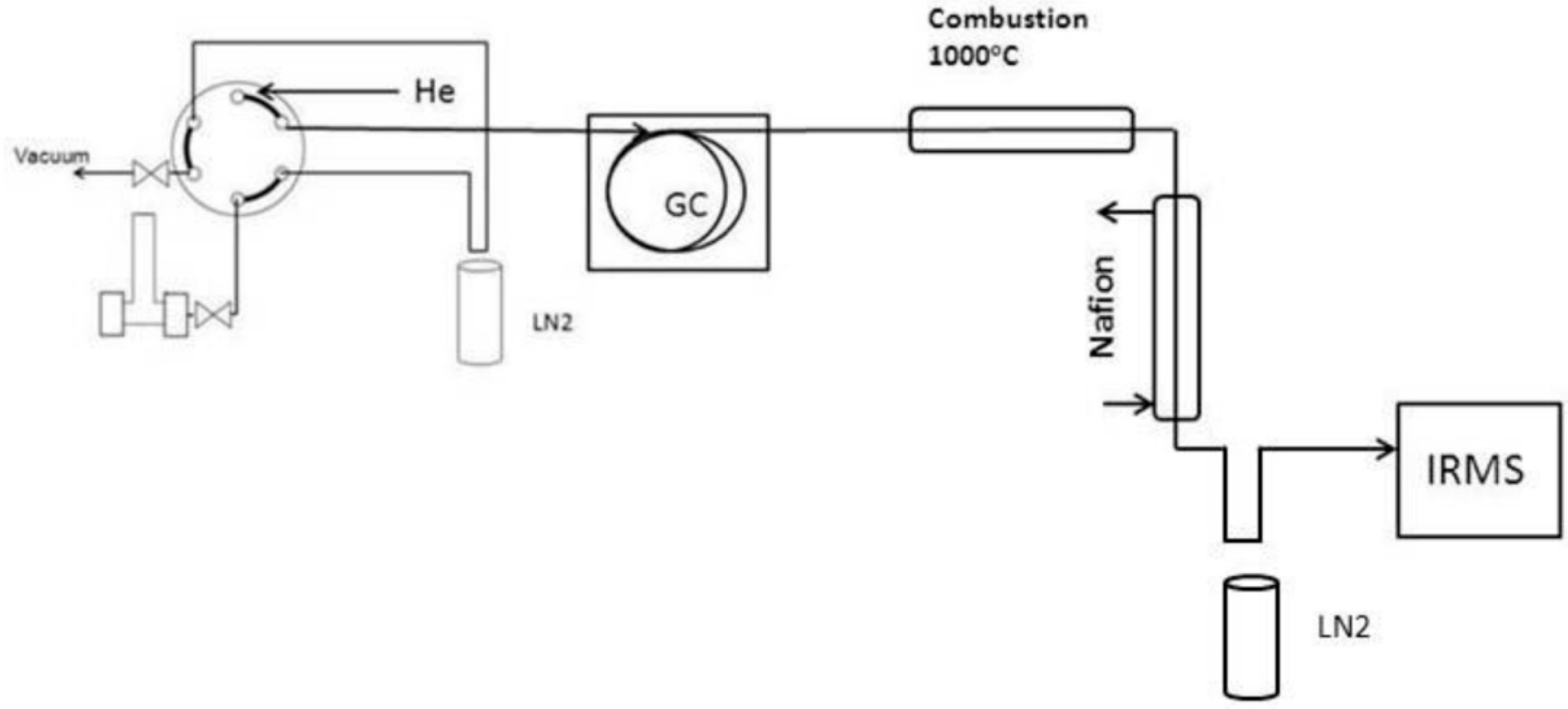
2.2. Analytical Methods

The original core samples were homogenized and pyrolyzed using Rock-Eval 6 to obtain the following data: TOC (%), T_max (°C), S₁, S₂ (mg HC/g rock), S₃ (mg CO₂/g rock), and derived parameters HI (mg HC/g TOC) and OI (mg CO₂/g TOC). Polished surfaces were prepared from rock chips for the random reflectance (R_r) measurement. This was carried out in oil under non-polarized light using the Opton Zeiss microscope photometer with 50× and 100× objectives and optical standards of 0.58%, 0.89%, 1.71%, and 3.12%.

Samples for the measurement of elemental and carbon isotope composition were homogenized to 60 μm and acidified by 10% hydrochloric acid to remove carbonates; then, they were washed repeatedly with distilled water and dried. The samples so treated were measured for the content of organic C and δ¹³C using flash combustion in a Fisons 1108 elemental analyzer coupled with a Delta V isotope ratio mass spectrometer (both products were from Thermo Scientific) in a continuous flow regime with NBS 22 (for δ¹³C measurement) and acetanilide (for elemental analysis) as reference materials. The standard error of carbon content measurement is about 3% from the measured value; the external reproducibility of δ¹³C measurement was less than 0.1‰.

Samples for gas measurement were firstly crushed to obtain particles less than 2 mm in size; the dust was removed. Particles were further used for chemical and isotopic analysis. The volume, as well as the chemical composition, was determined by gas chromatography with a flame ionization detector (FID; GC 96, Labio). An internally constructed hammer mill (Figure 1) was filled with rock particles (0.6 to 0.8 g), closed, and washed out with helium as a carrier gas; then, the rock was crushed using a handheld hammer. After the rock was crushed, the mill was installed in the loop of a six-way valve (Valco P Series) and all of the gas content was introduced into a column (PoraPlot Q 0.53 mm inner diameter (ID), 30 m) with helium as a carrier gas (gas flow 4 mL/min). The chromatograph oven was maintained at 35 °C for 3 min and heated up to 120 °C with a gradient of 15 °C per min. The chromatograph was calibrated by a standard gas mixture (1% of methane, ethane, and propane in air, Linde Gas) with known FID reference factors for higher hydrocarbons. The inner volume of the hammer mill was about 2 mL. To transfer all the gas content from the mill to chromatograph, more than 1 min of loop elution was necessary, which resulted in peak splitting of separated hydrocarbons.

Each sample was crushed and measured twice—once for the gas content and, consequently, a second time for ¹³C isotope measurement. For isotope analysis, we only used a part of the mill volume to maintain a good peak resolution on Trace GC (PoraPlot Q capillary 0.3 mm ID, 30 m with 1.8 mL/min flow rate). The chromatograph oven was maintained at 35 °C for 3 min and heated up to 120 °C with a gradient of 15 °C per min. The six-way valve (Valco P Series) was installed on the Trace GC inlet with a sampling loop (200–300 μL). The loop was evacuated, and part of the mill gas content (from 10–15%) was transferred to the loop. After loop change, the gas content was introduced to a GC inlet, Isolink combustion unit, and Delta V isotope mass spectrometer (all Thermo Scientific). Reference methane mixtures (T iso2, L iso1 produced by Isometric Instruments, Victoria, Canada) were used for calibration. Limited loop volume reduced the sample size, but the δ¹³C measurement was well reproducible (repeated sample crushing with following isotope analysis differed in δ¹³C by 0.5‰, Figure 2).

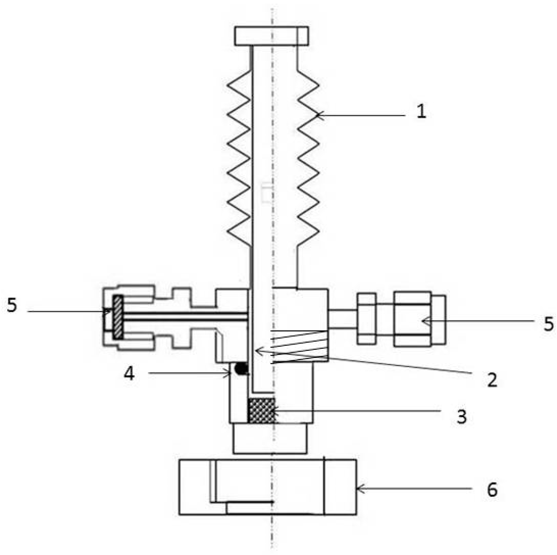
2.3. The Mechanism of Gas Release

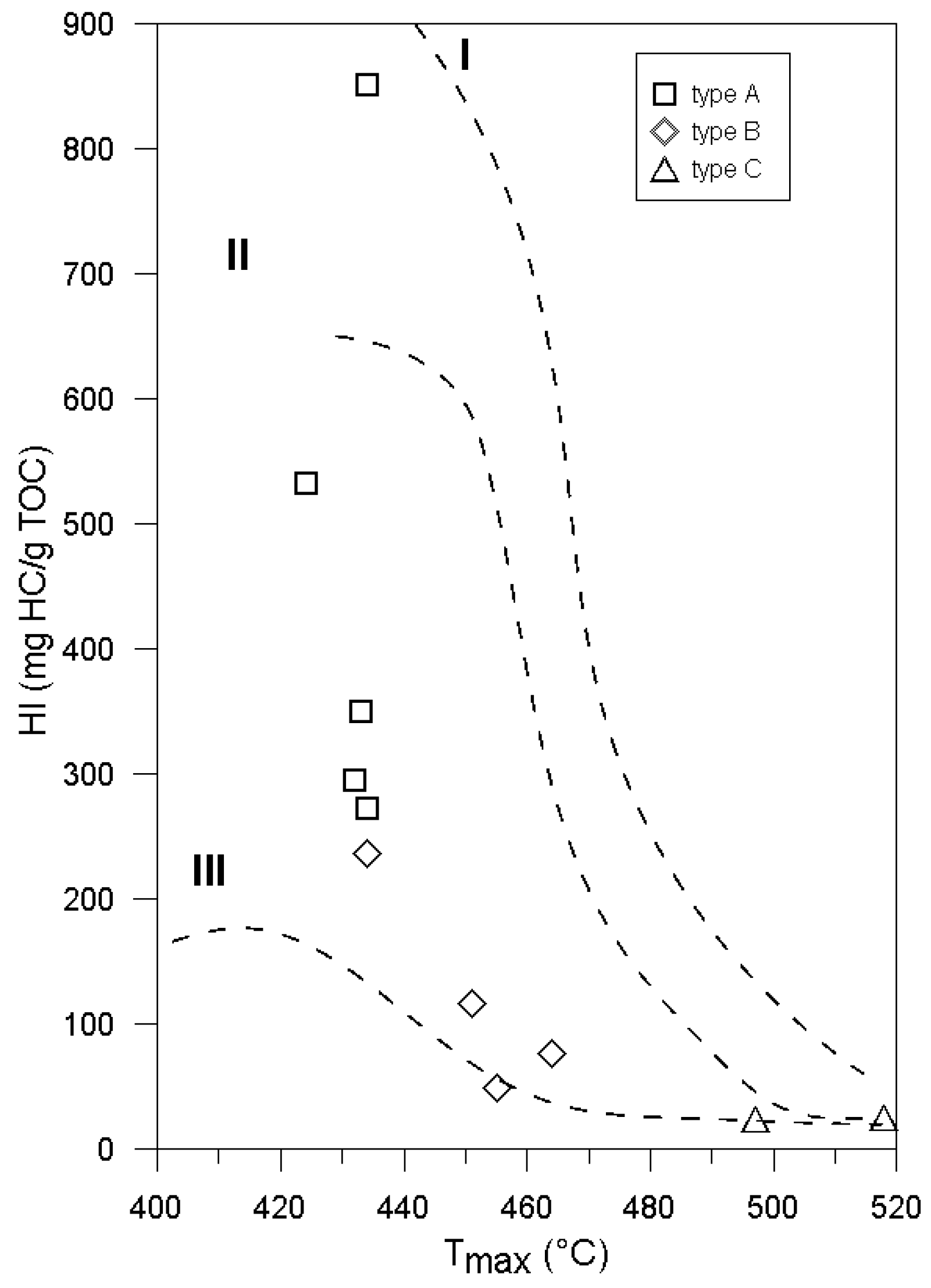
Stored shale samples lost part of the available gas via desorption and diffusion. Diffusion flux N_i is given by Fick’s first law, which only depends on the interaction of the solute substance i within the solvent environment [19]. The diffusion coefficient D_i defines the molar flux through a surface per unit concentration gradient out of plane.

N_i = −D_i grad c_i

(1)

For methane, the air diffusion coefficient is 1.6 10⁻⁵ m²∙s⁻¹ [20]. Diffusion coefficients of higher hydrocarbons are lower according to their higher molecular mass and molecular size. Values can be derived from the methane diffusion coefficient D_AM and molecular masses according to Graham’s law [20].

D_AM/D₂ = √(M₂/M_CH4)

(2)

The corresponding diffusion coefficients for ethane, propane, and butane would be 1.6.10⁻⁵ m²∙s⁻¹ divided by 1.15, 1.4, and 1.6. The diffusion of gases in porous media is directed by effective diffusion coefficients D_eff, which are many orders of magnitude less than the diffusion coefficient D_AM for methane in pure air [19], because of the tortuosity of porous media and retardation.

D_eff = D_AM × R × τ

(3)

where τ is the tortuosity factor (τ < 1), and R is the retardation coefficient (R >> 1). The diffusing substance can adsorb onto the internal surface of the porous medium. The adsorption/desorption process has a complicated effect on the degassing rate due to the delay of mass transport [11]. Hydrocarbon mobility through the rock is strongly reduced by organic matter content [8,9]. Considering a low adsorption affinity of methane to organic matter in comparison with higher hydrocarbons [9], higher hydrocarbons would be significantly retarded in diffusion compared to methane. In this way adsorption/desorption processes further enlarge the retardation of the diffusion of higher hydrocarbons vs. methane in comparison with Graham’s law [20].

The actual isotopic ratio R = ¹³C/¹²C changes during a single unidirectional process of diffusion by a fractionation factor α = D_m^H/D_m^L (where D_m is the diffusion coefficient of substance m with heavy H and light L isotopes, α < 1). The experimental isotope enrichment factor ε during kinetic fractionation can be determined using the Rayleigh equation [21].

1000 × ln R/R₀ = 1000 × ln (δ¹³C/1000 + 1)/(δ¹³C₀/1000 + 1) = ε × ln C/C₀

(4)

where R refers to the ratio ¹³C/¹²C, δ¹³C₀ and δ¹³C refer to the initial isotope ratio of a compound and the isotope ratio at time t, respectively, and C₀ and C are the initial concentration and the concentration at time t, respectively. Ratio C/C₀ is the fraction of an unreacted (or not released in this case) compound from the surface, frequently assigned as f. In analogy with the ‰ notation of δ, the enrichment factor ε is evaluated as the enrichment of the residual compound against the initial composition in ‰ units; ε = (α − 1) × 1000. During kinetic fractionation, the light isotopes are preferentially released from the rock surface, which is progressively enriched in heavy isotopes.

To express changes in the chemical composition of the residual gas during migration, we used a simplified heuristic approach. In gas mixtures, methane is the most abundant component, forming about 90 vol.% or more [1]. Higher gaseous hydrocarbons (ethane, propane, and butane) contribute only in units of percentage. Moreover, methane is less retarded by adsorption/desorption phenomena in pore transport, in comparison with higher hydrocarbons [9,22]. As the first approximation in the calculation of the gas loss, we suppose that methane is the only gas lost from the rock. The proceeding methane loss generates changes in the chemical composition of remaining gas components (see Figure 3).

To find a common solution for the entire sample subset (i.e., for the formations A, B, and C), we assume that we analyzed one sample in a different stage of the gas loss. For the modeling of the changes in gas composition with proceeding methane loss, an estimation of the initial gas composition was necessary. We approximated the gas composition by the actual gas composition from a similar rock formation or by composition from existing drilling mud. We used a model initial composition No. 1 (90% of C1, 4% of C2, 3% of C3, 2% of C4, and 1% of C5) for set A and B, and mixture No. 2 (95% of C1, 2.5% of C2, 1% of C3, 1% of C4, and 0.5% of C5) for set C. The chemical composition of mixtures after modeled methane losses was compared with the chemical composition of gases released from samples to estimate their methane loss.

For example, the loss of 50% of initial methane from mixture No.1 develops a new mixture with the composition of 81.8% C1, 7.3% C2, 5.5% C3, 3.6% C4, etc. Such a mixture would have a C/C₀ ratio (Equation (4)) equal to 0.5. When we plot the modeled composition data together with measured data, we can estimate probable methane loss and residual methane concentration C for the samples (Figure 3). The initial methane concentration C₀ is substituted by the initial value of models, i.e., 90% or 95%. Finally, we can calculate the ratio of C/C₀ and isotope fractionation for gas loss according to Equation (4). Measured gas content data (Table 2) were plotted against C/C₀ and extrapolated to 1 to get the initial gas content V₀ in Table 3.

3. Results

Data from Rock-Eval (T_max, TOC, S₁, S₂, HI, OI) and reflectance measurements (R_r) were complemented with those obtained from the elemental analysis (organic carbon content and δ¹³C of organic carbon). According to the S₁ and S₂ values, samples of Mikulov Marls were just on the immature/mature border of the source rock classification (S₁ < 0.07–0.23 mg of HC/g rock, S₂ = 3.8–8.2 mg HC/g rock) with a production index (PI) less than 0.10, which corresponded to the low maturity of organic matter [3].

Samples of Ostrava Formation had lower values of S₁ (0.04–0.12 mg of HC/g rock) and S₂ (0.5–3.5 mg HC/g rock) parameters, but a slightly higher production index (PI) compared with Mikulov Marls. This was due to the higher maturity of Ostrava Formation samples (0.64–1.20% R_r, T_max = 434–464 °C) compared with 0.62–0.72% R_r and T_max not over 434 °C in Mikulov Marls. Samples from Liteň Formation with T_max 497 and 519 °C were those most thermally mature. Higher thermal maturity was also reflected in increased graptolite reflectance (1.79% R_r). The different kerogen types presented in each of the studied formations were evident in the HI versus T_max graph (Figure 4). A comparison of the bulk parameters proved the highest hydrogen index and the lowest maturity for Mikulov Formation, low HI for Ostrava and Liteň Formations, and the highest maturity for Liteň Formation.

Due to the high homogeneity of the depositional environment, the samples within the sub-groups A, B, and C were considered as representative of the same thermal maturity level and the same original organic matter (δ¹³C), despite the fact they originated from different depths (

Table 1. Geochemical parameters of the studied shales. Source rock (SR) classification based on measured total organic carbon (TOC) calculation values according to Reference [23]. HI—hydrogen index; SR—source rock; PI—production index; R_r—random reflectance.

Sample	Corg (%)	δ13C (‰)	TOC Calculated (%)	Tmax (°C)	S2 (mg HC/g Rock)	S1 (mg HC/g Rock)	HI (mg HC/g TOC)	OI (mg CO2/g TOC)	SR Type	PI = S1/(S1 + S2)	Rr (%)
A	2.56	−26.7	1.46	432	4.31	0.11	295	47	Very good	0.02	0.69
A	2.44	−27.2	1.39	434	3.78	0.09	272	22	Very good	0.02	0.72
A	2.47	−26.8	1.23	433	4.30	0.07	350	33	Very good	0.02	0.68
A	3.57	−26.7	0.96	434	8.17	0.23	851	90	Very good	0.03	0.65
A	0.74	−24.3	2.4	424	12.79	0.23	533	29	Fair	0.02	0.66
B	1.08	−23.1	1.09	455	0.52	0.04	48	26	Good	0.07	1.20
B	4.57	−24.2	1.48	434	3.50	0.12	236	13	Very good	0.03	0.64
B	1.45	−24	1.44	451	1.60	0.08	117		Good	0.05	1.00
B	0.98	−24.5	1.67	464	1.20	0.08	77		Good	0.06	1.05
C	3.18	−31.5	3.89	501	1.00	0.05	27	1	Very good	0.05	1.79
C	3.18	−30.4	3.89	518	0.90	0.06	25	1	Very good	0.06
C	5.69	−29.8	6.32	504	1.35	0.07	22	1	Very good	0.05
C	3.26	−30	5.07	497	1.10	0.09	23	1	Very good	0.08
Ex	6.43	−29	2.59	455	1.65	0.44	24	0	Very good	0.21

).

We tested samples for the gas content, as well as chemical and ¹³C isotope composition (see

Table 2. Chemical and δ¹³C isotopic composition of gases extracted from the crushed archived shales.

Sample	Depth (m)	Gas Volume (m3∙t−1)	C1 (%)	δ13C1 (‰)	C2 (%)	δ13C2 (‰)	C3 (%)	δ13C3 (‰)	C4 (%)	δ13C4 (‰)
A	3342	0.00050	48.5	−19.6	14.8	−20.6	24.4		10.9
A	3491	0.00065	74.1	−22.4	9.6	−21.4	7.2	−21	6.3
A	2997	0.00045	48.4	−18.8	17.8	−17.9	20.7		10.3
A	3411	0.00055	55.5	−18.4	12.6	−16.9	18.3		10.1
A	2546	0.00090	81.3	−26.5	10.4	−24.6	4.6		1.8
B	4575	0.00040	55.5	−23.7	14.1	−22.3	17.3	−23	10
B	4034	0.00017	38.0	−18.8	20.0	−19.8	24.4		14
B	1374	0.00015	29.2	−14.6	29.2	−21.5	35.3		6.3
B	4760	0.00030	32.3	−16.0	13.9	−20	13		22.8
C		0.0014	58.2	−22.0	8.6	−19.4	10		10
C		0.0006	67.0	−21.3	9.2	−21	10.5	−23	7.8
C		0.0125	95.0	−27.9	2.0	−22	1		0.8
C		0.0078	86.0	−26.0	8.9		1.5		1.8
Ex		0.0239	44	−24.2	26	−25.2	12	−25	10	−24

). The volume of the gas released from the sample in the mill was calculated as a sum of volumes from C1 to C4. The volume of the released gas was very variable, as was the chemical composition of gases. The C1 content of samples was lower than C1 of model mixtures (from 80% to 20%); the content of C2–C4 was higher (from 2 to 29%). Generally, the gas composition of released gases follows the effect of the methane loss on the composition of the gas mixture; increasing methane loss increases the contribution of higher hydrocarbons up to tens of percent (Figure 3). Experimental data were close to modeled gas composition with a few exceptions. One sample from B and one sample from C had a significantly higher concentration of C2 and C3 than the model (Figure 3). Considering the chemical composition of the model for the initial gas composition (90% of C1, 4% of C2, 3% of C3, 2% of C4, and 1% of C5 for B; 95% C1 for C), an initial composition of such a sample would probably be more abundant in methane than the model supposed. Unexpected were the values of the C3 concentration, which were generally higher than the C2 values (Table 2). This resulted from the simplified assumption of methane loss only. Obviously, samples also lost ethane, which resulted in the suppression of C2 concentration and an increase in C3 content.

From the measured δ¹³C, we calculated ¹³C fractionation during methane release (diffusion accompanied by desorption, according to Equation (4); see Figure 5). The necessary C and C₀ values for methane were calculated directly from the difference of the initial model concentration (C₀) and estimated methane loss (C = C₀ − loss). The evident loss of ethane was in contradiction with the assumption of methane loss only. The isotopic composition of ethane changed with the changes in chemical composition, and we clearly observed a similar process to methane loss. To keep the assumption of methane loss valid, we assumed that methane released first, and ethane released successively. In this case, we could use the calculated ethane content after methane loss as the initial C20 concentration before ethane loss. Measured concentrations of C2 were nearly always lower than model values (with two or three exceptions, which are visible in Figure 3, highlighting the calculated changes in composition). The difference between the model value (i.e., C20) and measured C2 content was the estimate of the ethane loss. In this way, we could evaluate the C/C₀ ratio and calculate the fractionation for ethane release (Figure 5).

The apparent fractionation enrichment ε is related to the gas loss via diffusion (and desorption); the intercept assigns the initial autochthonous isotope composition of methane and ethane. Isotope fractionation data and the estimates of initial δ¹³C₀ are summarized in

Table 3. Apparent diffusion fractionation ε for C1 and C2 with calculated estimates of the initial isotope composition δ¹³C₀.

Formation	δ13C Rock (‰)	δ13C10 (‰)	ε C1 (‰)	δ13C20 (‰)	ε C2 (‰)	V0 Gas (m3∙t−1)
B	−24.1	−25.7	−2.9	−22	−3.7	0.00165
A	−26.9	−25.5	−3	−21.6	−2.7	0.0017
C	−30.6	−28.3	−2.7	−22.5	−3.1	0.0132
Ex *	−29	−31	−3	−26.8		0.200

* An arbitrary value of −3‰ was used for the calculation of δ¹³C₀.

.

The initial gas volume V₀ (in m³ of gas per ton of rock) was estimated from the extrapolated chromatography data to C/C₀ = 1. The gas content of formation C was approximately 10 times higher than for formations A and B. The comparative gas-prone sample from Poland contained significantly more gas than samples from formation C despite the uncertainty of the estimate. We tested only one sample of comparative shale Ex; thus, methane loss was estimated from the gas composition (Table 2).

The initial isotope composition δ¹³C₀ derived for methane and ethane (together with some measured δ¹³C values for propane) can be associated with the source rock (Figure 6).

The data found in Figure 6A indicate a close relationship between the source organic and gaseous products with a small isotopic separation between successive n-alkane homologues. The relationship between alkanes (Figure 6B) is linear for Ostrava Formation and the comparative sample from Poland. Samples from Mikulov and Liten Formations present so-called isotopic reversal, where the δ¹³C value of propane is less negative than the ethane value [25]. Isotopic reversal is interpreted by mixing of different sources [26], by water–hydrocarbon reactions [25], or by mixing of primary and secondary generated hydrocarbons [10].

Figure 6. The relationship between δ¹³C of the source rock and the shale gas components estimated from extrapolation of ¹³C fractionation to initial δ¹³C values (A). Diagram of 1/Cn versus δ¹³C for the same initial values according to Reference [26] (B).

Figure 6. The relationship between δ¹³C of the source rock and the shale gas components estimated from extrapolation of ¹³C fractionation to initial δ¹³C values (A). Diagram of 1/Cn versus δ¹³C for the same initial values according to Reference [26] (B).

4. Discussion

4.1. Estimate of Gas at the Site

We do not know the initial volumes of the gas at the site; thus, our estimates (Table 3) can be confronted only with other independent geochemical data (Table 1). According to References [3,4], studied shale samples have a potential for hydrocarbon production. The organic matter content was higher than a minimum of 0.5%; Rock-Eval index S₂ (thermal kerogen cracking) was within the range of units. In addition, methane δ¹³C values corresponded to the maturity of samples [27].

However, the S₁ index (volatile organic compounds) and production index PI = S₁/(S₁ + S₂), were low, which corresponded to a minimal degree of hydrocarbon production. In this way, it was consistent with a small volume of the gas released (in L per ton of rock). The organic matter in shales (A and B) was immature (T_max < 430 °C, 450 °C) and could not produce measurable amounts of hydrocarbons. Shales from Liteň (type C) had a higher T_max, which corresponded to higher maturity and the possibility of higher gas production (Table 3).

For comparison, we included a gas-prone sample from Poland. While this sample was comparable with group B in terms of thermal maturity, its PI index was higher (Table 1). This was also consistent with the content of gas released, which was well above the samples of group B.

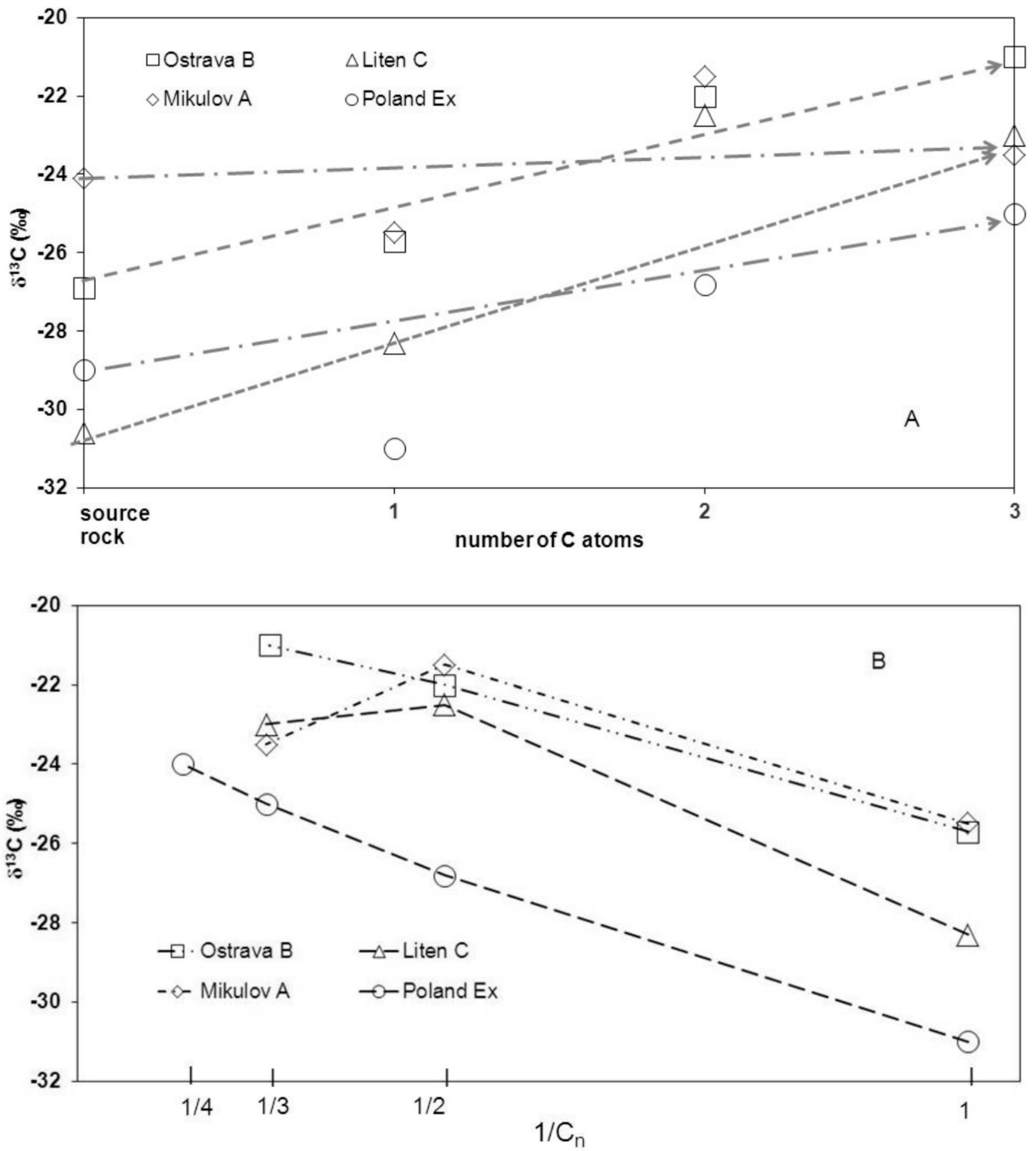
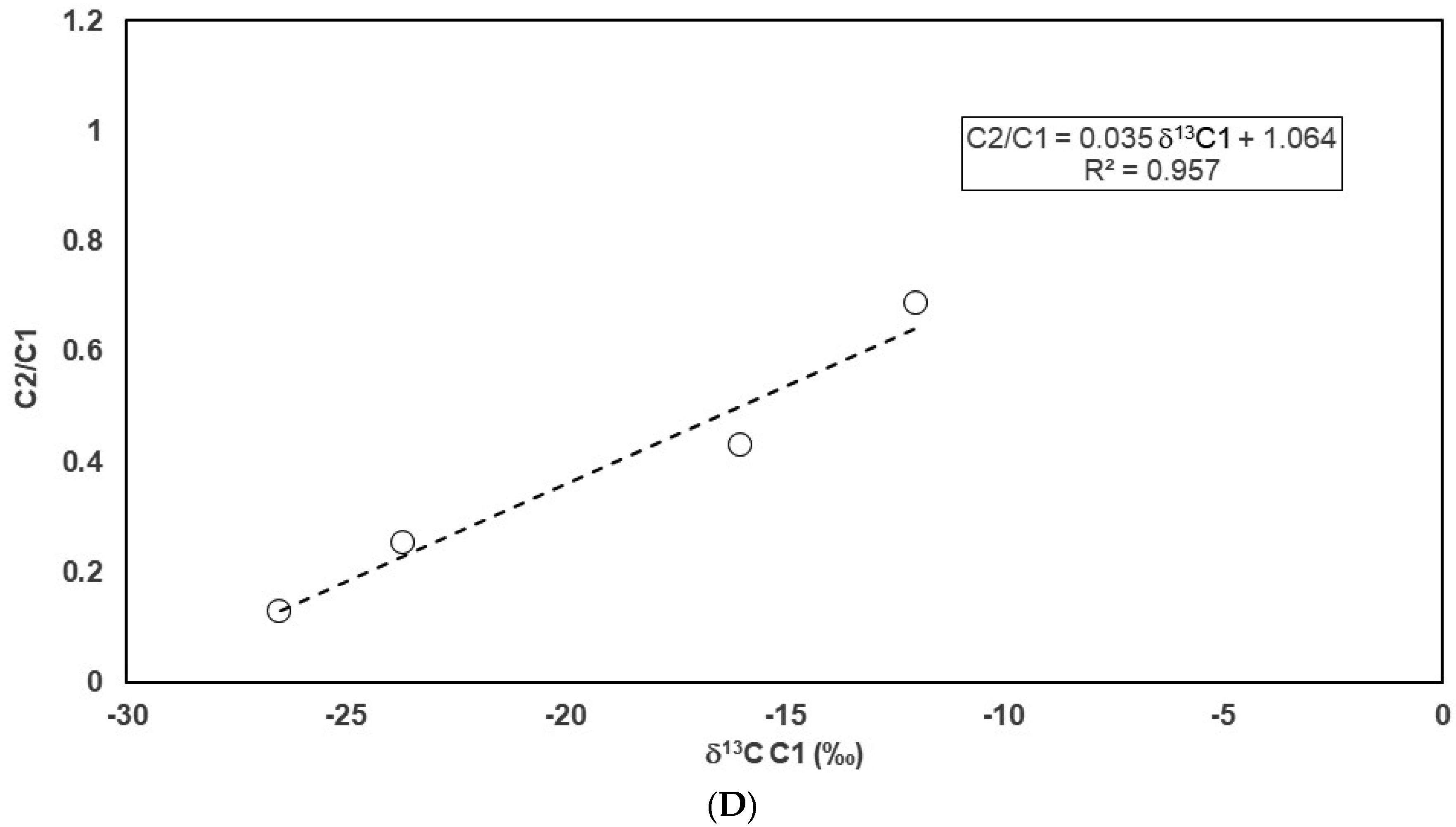
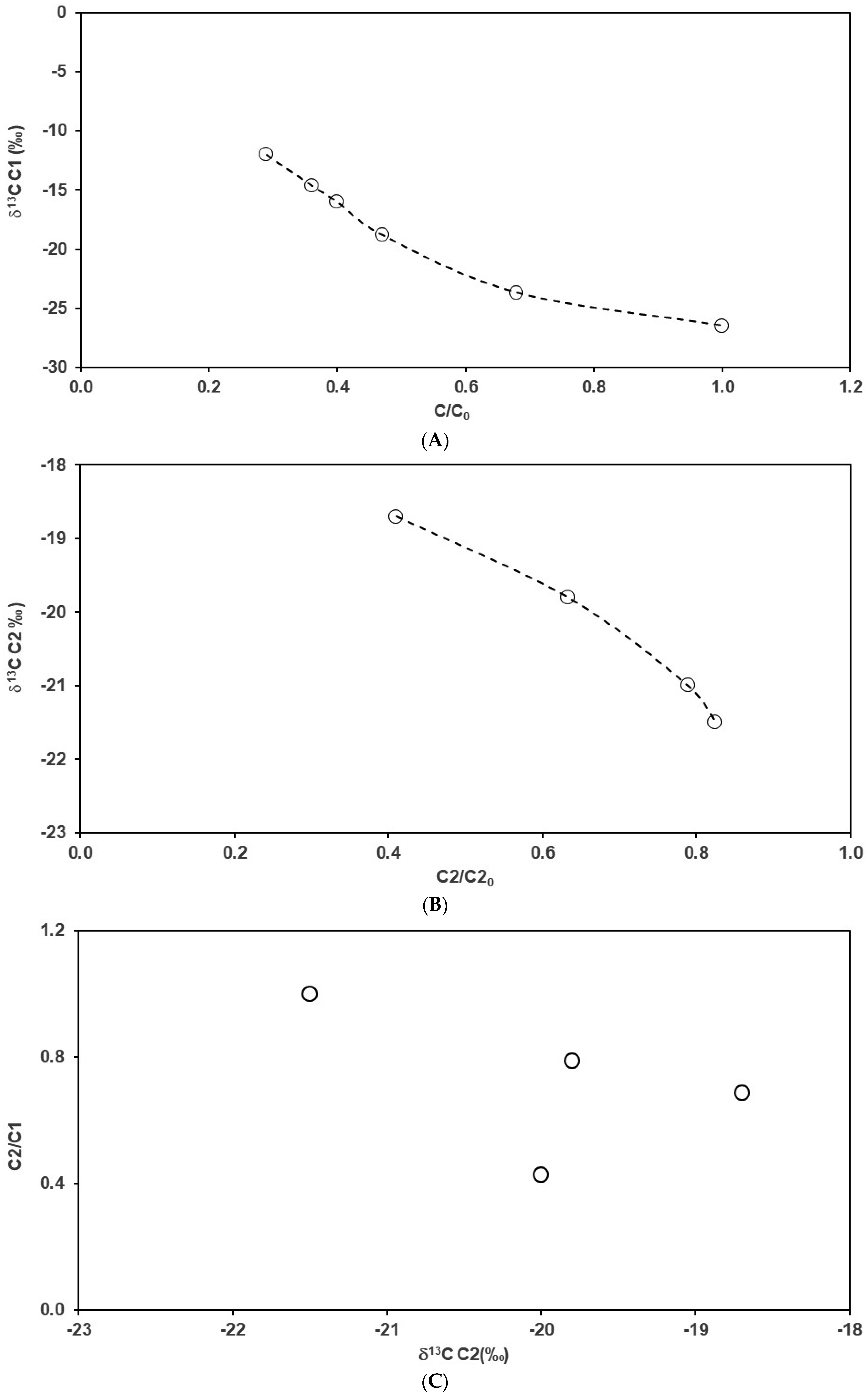
4.2. Carbon Isotope Fractionation during the Sample Degassing

We assumed that, for a given set of shales (A, B, or C), the hydrocarbon production proceeded to the same extent according to geochemical conditions, and the single samples differed by degassing loss only. The collected samples released gas based on their porosity, organic content, and duration of diffusion; sample size would also be important. As we could not evaluate samples separately with so many variables, we considered the entire set as a single sample with different degrees of degassing. In this way, the calculated isotope fractionation was similar to the results of the coal canister method [12]. Determined isotope enrichment ε = −3‰ for the methane release neared the −2‰ value for the methane desorption from coal [12,22] and the experimental values from Reference [9] (−1.6 to −2.8‰). The study referred to in Reference [8] reported values from −3.3 to −1.3 ‰ (−4 ‰ as a maximum for coal and mudstone).

The isotope enrichment determined for ethane release ε = −2.7 to −3.7‰ was larger than that measured for rock experiments (−0.8 to −1.6‰) [9]. Although quite different isotope fractionation values for both methane (−9.2‰) and ethane (−2.8‰) were reported in the experimental study in Reference [28], it is generally accepted that carbon isotope fractionation should decrease with increasing carbon number [9,29]. Results from diffusion modeling in Reference [11] were also similar. However, the secondary process as desorption could have had a significant effect on isotope fractionation, as was observed during coal bed gas production experiments [22]. We supposed that such secondary processes modified our ethane isotope fractionation, which was higher than literature values.

The observed isotopic reversal for propane ¹³C (Figure 6B) had no simple explanation. Considering the low maturity of measured samples, we could not suppose the formation of ethane/propane rollover, as it proceeds during gas production from highly mature shales [30], or by mixing of primary and secondary generated gases [10]. We have only few data on δ¹³C of propane available (Table 2), and solutions as admixtures of another gas or possible effects of preferential adsorption of ¹²C against ¹³C as reported in Reference [29] cannot be differentiated.

Propane isotopic reversal can also arise from the formation of the “heavy” ethane as we observed for the samples from Liten Formation (subset C). These samples had the highest TOC content (Table 1), which affected both the adsorption properties of shales and the carbon isotope fractionation during desorption. Isotope fractionation decreases during desorption with a decreasing content of TOC in the sample [8], while increasing the adsorption capacity increases isotope fractionation during methane desorption [11]. Desorption affects the isotopic composition of the expelled gas because the light isotopologue is preferentially desorbed. Finally, the gas residuum (which is released after rock crushing) is isotopically enriched.

5. Conclusions

Diffusion and adsorption/desorption processes affect the chemical and isotopic composition of residual gases in shale samples. We attempted to reconstruct the original gas content of shales from the gas residuum released from archived crushed-rock samples. Samples from the same formation, i.e., with the same geochemical parameters, differ in their gas content and composition because of different rock properties and sample history. To find a common solution for the entire set, we assume that we analyzed one sample in a different stage of gas loss. The main findings of the study were as follows: the ¹³C isotope fractionation ε for diffusion ranged between −2.7‰ and −3‰ for methane and between −2.7‰ and −3.7‰ for ethane. Estimated δ¹³C values of indigenous gas components (methane, ethane, and propane) were very near to the source rock value. The dominant processes influenced the estimates of δ¹³C values as follows: (i) the gas-abundant sample had a more negative δ¹³C of methane than the source rock because of diffusion, and (ii) the organic-rich rocks desorbed ethane slowly, which shifted the δ¹³C value of ethane to a value that was less negative than that for the source rock. Estimates of the original gas volume produced in situ were consistent with the maturity parameters of shales. Most of the shales were immature, and the gas volume ranged between 1 and 200 L per ton of rock. Methane was the dominant component of any lost gas. Archived shales lost 20% to 95% of the original methane. This resulted in an unusual chemical composition of the residual gases, which contained mostly higher hydrocarbons, with a quantity of tens of vol.%.

References

1. Chaelrs, B.; John, L.; Reberto, S.-R.; Richard, E.L.; George, W. Producing Gas from Its Source. Oilfield Rev. 2006, 18, 36–49. [Google Scholar]
2. John, B.C. Fractured shale-gas systems. AAPG Bull. 2002, 86, 1921–1938. [Google Scholar]
3. Petroleum Formation and Occurrence; Tissot, B.P.; Welte, D.H. (Eds.) Springer: Heidelberg, Germany, 1984. [Google Scholar]
4. Peters, K.E. Guidelines for Evaluating Petroleum Source Rock Using Programmed Pyrolysis. AAPG Bull. 1986, 70, 318–329. [Google Scholar]
5. Schoell, M. Genetic Characterization of Natural Gases. AAPG Bull. 1983, 67, 2225–2238. [Google Scholar]
6. Tang, Y.; Jenden, P.D.; Nigrini, A.; Teerman, S.C. Modeling Early Methane Generation in Coal. Energy Fuels 1996, 10, 659–671. [Google Scholar] [CrossRef]
7. Tang, Y.; Perry, J.K.; Jenden, P.D.; Schoell, M. Mathematical modeling of stable carbon isotope ratios in natural gases. Geochim. Cosmochim Acta 2000, 64, 2673–2687. [Google Scholar] [CrossRef]
8. Zhang, T.; Krooss, B.M. Experimental investigation of the carbon isotope fractionation of methane during gas migration by diffusion through sedimentary rocks at elevated temperature and pressure. Geochim. Cosmochim. Acta 2001, 65, 2723–2742. [Google Scholar] [CrossRef]
9. Schloemer, S.; Krooss, B.M. Molecular transport of methane, ethane and nitrogen and the influence of diffusion on the chemical and isotopic composition of natural gas accumulations. Geofluids 2004, 4, 81–108. [Google Scholar] [CrossRef]
10. Goddard, W.A., III; Tang, Y.; Wu, S.; Deev, A.; Ma, Q.; Li, G. Novel Gas Isotope Interpretation Tools to Optimize Gas Shale Production; Report Number 08122.15; Californian Institute of Technology: Pasadena, CA, USA, 2013. [Google Scholar]
11. Xia, X.; Tang, Y. Isotope fractionation of methane during natural gas flow with coupled diffusion and adsorption/desorption. Geochim. Cosmochim. Acta 2012, 77, 489–503. [Google Scholar] [CrossRef]
12. Strąpoć, D.; Schimmelmann, A.; Mastalerz, M. Carbon isotopic fractionation of CH4 and CO2 during canister desorption of coal. Org. Geochem. 2006, 37, 152–164. [Google Scholar] [CrossRef]
13. Zhang, T.; Yang, R.; Milliken, K.L.; Ruppel, S.C.; Pottorf, R.J.; Sun, X. Chemical and isotopic composition of gases released by crush methods from organic rich mudrocks. Org. Geochem. 2014, 73, 16–28. [Google Scholar] [CrossRef]
14. Geršlova, E.; Opletal, V.; Sýkorová, I.; Sedláková, I.; Geršl, M. A geochemical and petrographical characterization of organic matter in the Jurassic Mikulov Marls from the Czech Republic. Int. J. Coal Geol. 2015, 141, 42–50. [Google Scholar] [CrossRef]
15. Geršlová, E.; Goldbach, M.; Geršl, M.; Skupien, P. Heat flow evolution, subsidence and erosion in Upper Silesian Coal Basin, Czech Republic. Int. J. Coal Geol. 2016, 154, 30–42. [Google Scholar] [CrossRef]
16. Suchy, V.; Sýkorová, I.; Stejskal, M.; Safanda, J.; Machovič, V.; Novotná, M. Dispersed organic matter from Silurian shales of the Barrandian Basin, Czech Republic: Optical properties, chemical composition and thermal maturity. Int. J. Coal Geol. 2002, 53, 1–25. [Google Scholar] [CrossRef]
17. Picha, J.F.; Stranik, Z.; Krejci, O. Geology and hydrocarbon resources of the outer West Carpathians and their foreland, Czech Republic. In The Carpathians and Their Foreland: Geology and Hydrocarbon Resources; Golonka, J., Picha, J.F., Eds.; American Association of Petroleum Geologists (AAPG) Memoirs: Tulsa, OK, USA, 2006. [Google Scholar]
18. Sedláková, I.; Geršlová, E.; Uhlík, P.; Opletal, V. Mineralogical characteristics of upper Jurassic Mikulov Marls, the Czech Republic, in relation to their thermal maturity. Geochemie der Erde 2017, 77, 159–167. [Google Scholar] [CrossRef]
19. Transport Modeling for Environmental Engineers and Scientists; Clark, M.M. (Ed.) Wiley: Hoboken, NJ, USA, 2009. [Google Scholar]
20. Chemodynamics: Environmental Movement of Chemicals in Air, Water, and Soil; Louis, J.T. (Ed.) Wiley: Hoboken, NJ, USA, 1979. [Google Scholar]
21. Handbook of Environmental Isotope Geochemistry, vol. 1 a, Terrestrial Environment; Fritz, P.; Fontes, J.C. (Eds.) Elsevier: Amsterdam, The Netherlands, 1980. [Google Scholar]
22. Niemann, M.; Whiticar, M.J. Stable Isotope Systematics of Coalbed Gas during Desorption and Production. Geoscience 2017, 7, 43. [Google Scholar] [CrossRef]
23. Bacon, C.A.; Calver, C.R.; Boreham, C.J.; Leaman, D.E.; Morrison, K.C.; Revill, A.T.; Volkman, J.K. The petroleum potential of onshore Tasmania: A review. Geol Survey Bull. 2000, 71, 1–93. [Google Scholar]
24. Prinzhofer, A.; Pernaton, E. Isotopically light methane in natural gas: Bacterial imprint or diffusive fractionation? Chem. Geol. 1997, 142, 193–200. [Google Scholar] [CrossRef]
25. John, Z.; Kevin, F.; Stephen, B. Isotopic reversal (“rollover”) in shale gases produced from the Mississipian Barnett and Fayetteville formations. Mar. Petrol. Geol. 2012, 31, 43–52. [Google Scholar]
26. Chung, H.; Gormly, J.; Squires, R. Origin of gaseous hydrocarbons in subsurface environments: Theoretical considerations of carbon isotope distribution. Chem. Geol. 1988, 71, 97–104. [Google Scholar] [CrossRef]
27. Berner, U.; Faber, E. Empirical carbon isotope/maturity relationships for gases from algal kerogens and terrigenous organic matter, based on dry, open-system pyrolysis. Org. Geochem. 1996, 24, 947–955. [Google Scholar] [CrossRef]
28. Meng, Q.; Wang, X.; Wang, X.; Zhang, L.; Jiang, C.; Li, X.; Shi, B. Variation in the carbon isotopic composition of alkanes during shale gas desorption process and its geological significance. J. Nat. Gas Geosci. 2016, 1, 139–146. [Google Scholar] [CrossRef]
29. Strapozc, D.; Michael, G.E.; Roper, J.; Maguire, M. Insight into shale gas production & storage from gas chemistry—what is it telling us? In Proceedings of the AAPG Hedberg Conference, Austin, TX, USA, 5–10 December 2010. [Google Scholar]
30. Hao, F.; Zou, H. Cause of shale gas geochemical anomalies and mechanisms for gas enrichment and depletion in high-maturity shales. Mar. Petrol. Geol. 2013, 44, 1–12. [Google Scholar] [CrossRef]
Figure 1. Sketched hammer mill. Below (1), the mill has an inner diameter of 8 mm. There is a mill hammer (2) inside. A sample of the rock (3) is placed in the lower part of the mill, sealed with an O-ring (4). The tubes (inner diameter: 1/16 inch) end with Swagelok tube fittings with septa (5). The mill is complete with a sealing nut (6).
Geosciences 09 00481 g001
Figure 2. Hydrocarbon combustion line. The sample loop is evacuated and connected to the hammer mill, and part of the mill content is transferred to the loop. The gas from the loop is injected into the gas chromatograph. The loop can be immersed in liquid nitrogen to concentrate higher hydrocarbons. Hydrocarbons are separated inside Trace GC.
Geosciences 09 00481 g002
Figure 3. Calculated changes in the chemical composition of the residual gas with increasing methane loss for the model gas mixture No. 1 and experimental data of Mikulov and Ostrava formations (A), and for model gas mixture No. 2 and data of the Liten formation (B).
Geosciences 09 00481 g003
Figure 4. The modified van Krevelen plot with hydrogen index (HI) versus thermal maturity (Tmax), which enables discerning the prevailing kerogen type of the studied source rocks.
Geosciences 09 00481 g004
Figure 5. (A) Plot of methane C/C0 ratio versus δ13C1. Initial C0 concentration corresponds with the initial methane content of the model gas composition No.1; (B) Plot of ethane C/C0 ratio versus δ13C2. Initial C0 concentration originates from the initial ethane content of the model gas mixture No.1; (C) Diagram C2/C1 versus δ13C1 according to [24]. Plot corresponds to linear mixing rather than diffusion loss. Possible two mixing members have δ13C1 −30 and −5‰ (Ostrava Formation—subset B); (D) Diagram C2/C1 versus δ13C2. Linear mixing is not positive, significant loss of methane overlap possible relationship (subset B).
Geosciences 09 00481 g005aGeosciences 09 00481 g005b