Tilting and Flexural Stresses in Basins Due to Glaciations—An Example from the Barents Sea

Abstract
1. Introduction
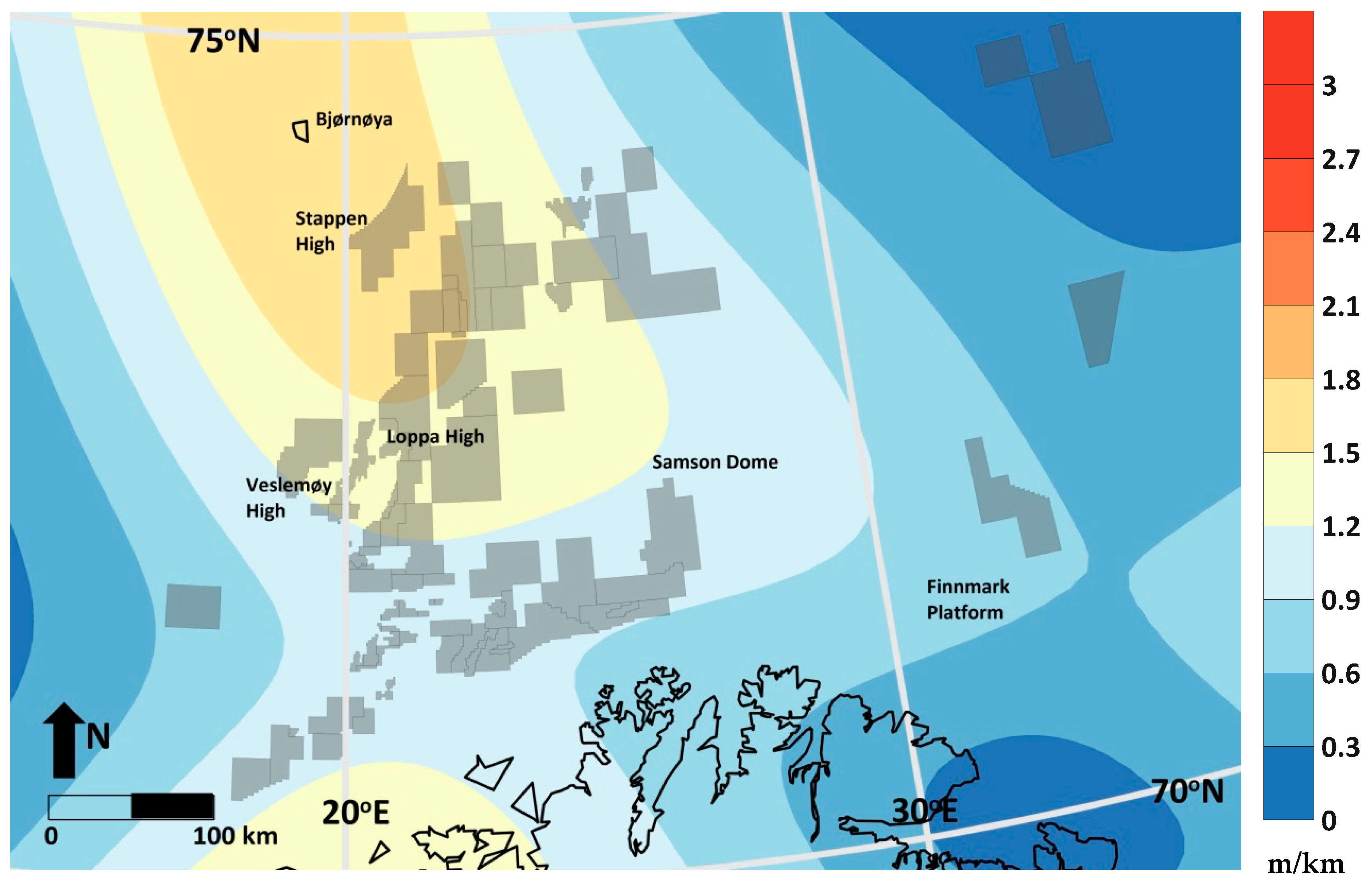
- Possible glacially induced tilting of reservoirs. Here, we calculate the glacially induced tilting of the Norwegian Continental Shelf due to the last ice age, with particular focus on the SW Barents Sea.
- Assessment of the flexural stresses induced by the lithospheric flexure related to glacial isostasy and tilt, and their effect on faults during glaciations and interglacials, here illustrated by an example from the SW Barents Sea where the stress modelling is limited to the flexural stress effects of deglaciation after LGM. The stress effects of vertical ice load and related stress migration are not calculated here.
2. Glaciations
2.1. Ice Thickness
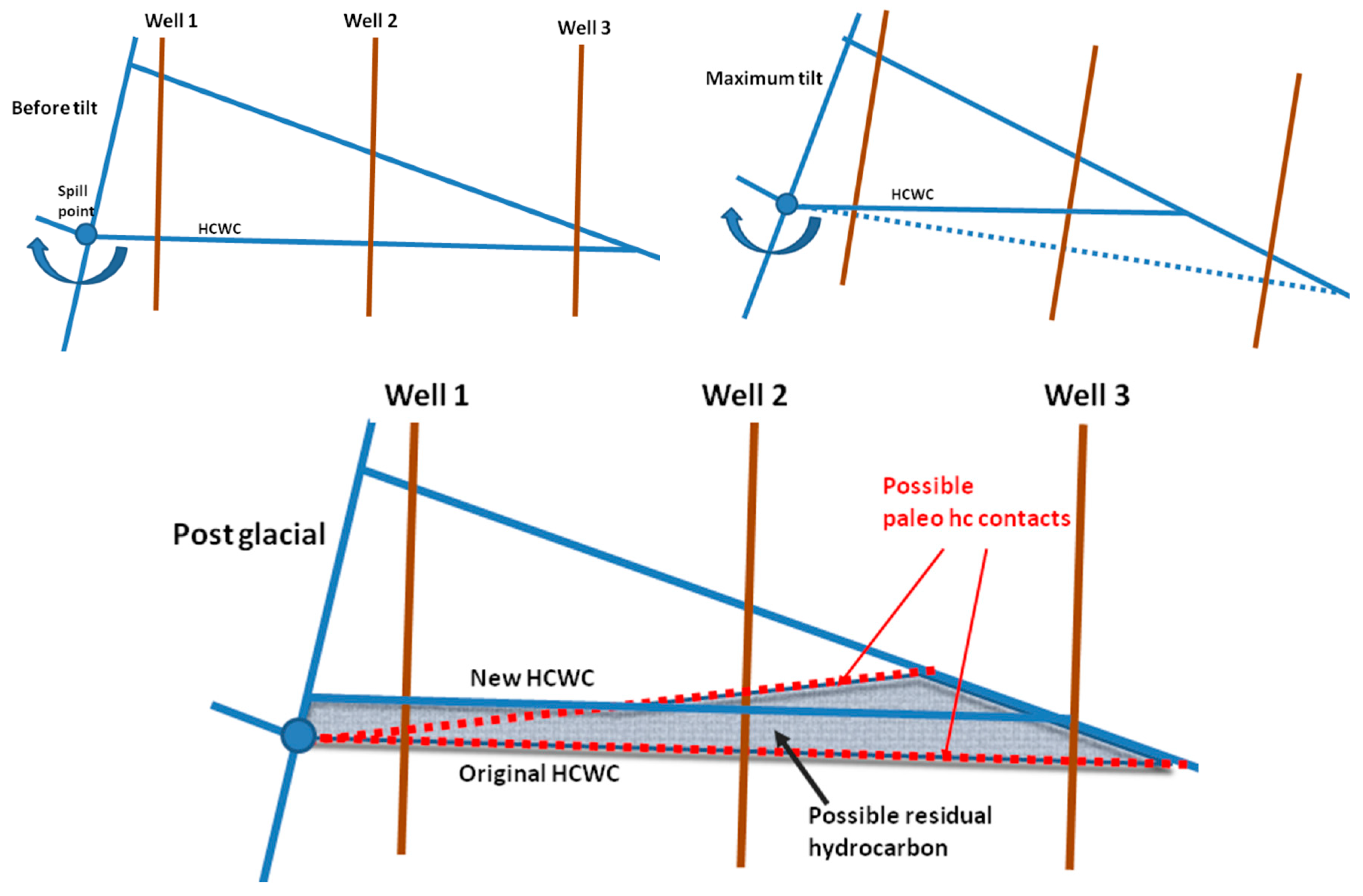
2.2. Glacial Isostasy and Tilting of Reservoirs
- The number of glacial events. Tilting will result from each isostatic event. A number of glacial events will create chaotic patterns of paleo contacts and residual oil which will be very difficult to interpret.
- The geometry of the receiving area. If a saddle area is opened, the fluids can migrate into higher lying traps or be lost to the surface. A surrounding flat area, on the other hand, can become part of the trap during the subsidence, and fluid can migrate back into the trap under uplift.
- Additional potential factors that determine the migration effect are: i) the geometry of the deformation, ii) the geometry of the hydrocarbon filled structures, iii) the initial fill of the trap, and iv) the spill point location and orientation of the structure.
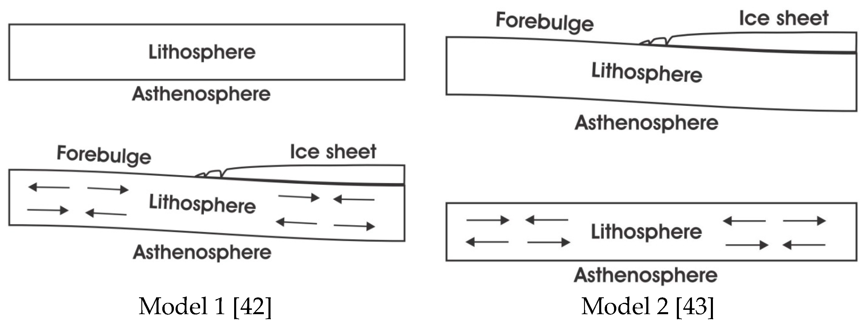
3. Flexure-Related Stress Effects
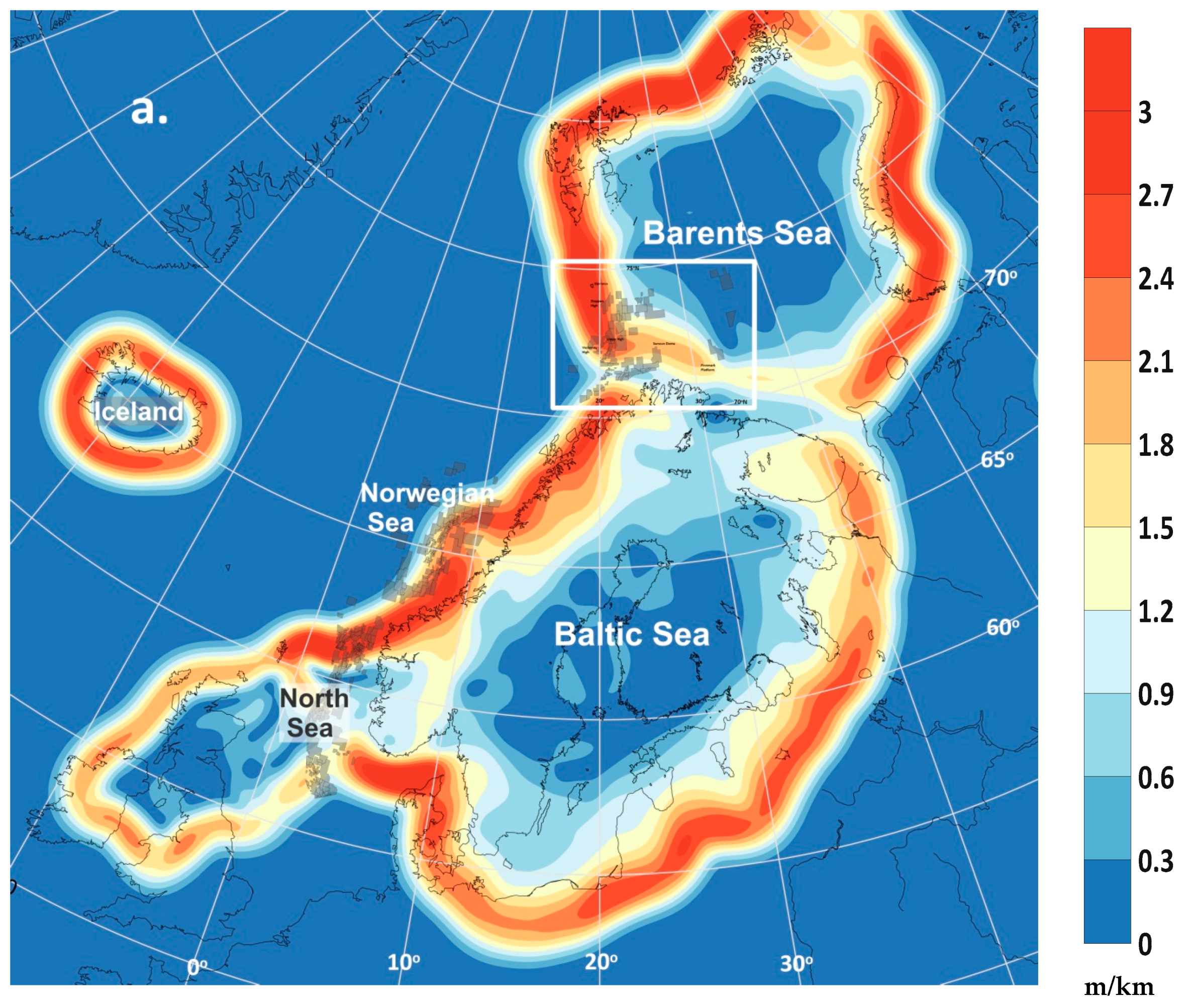
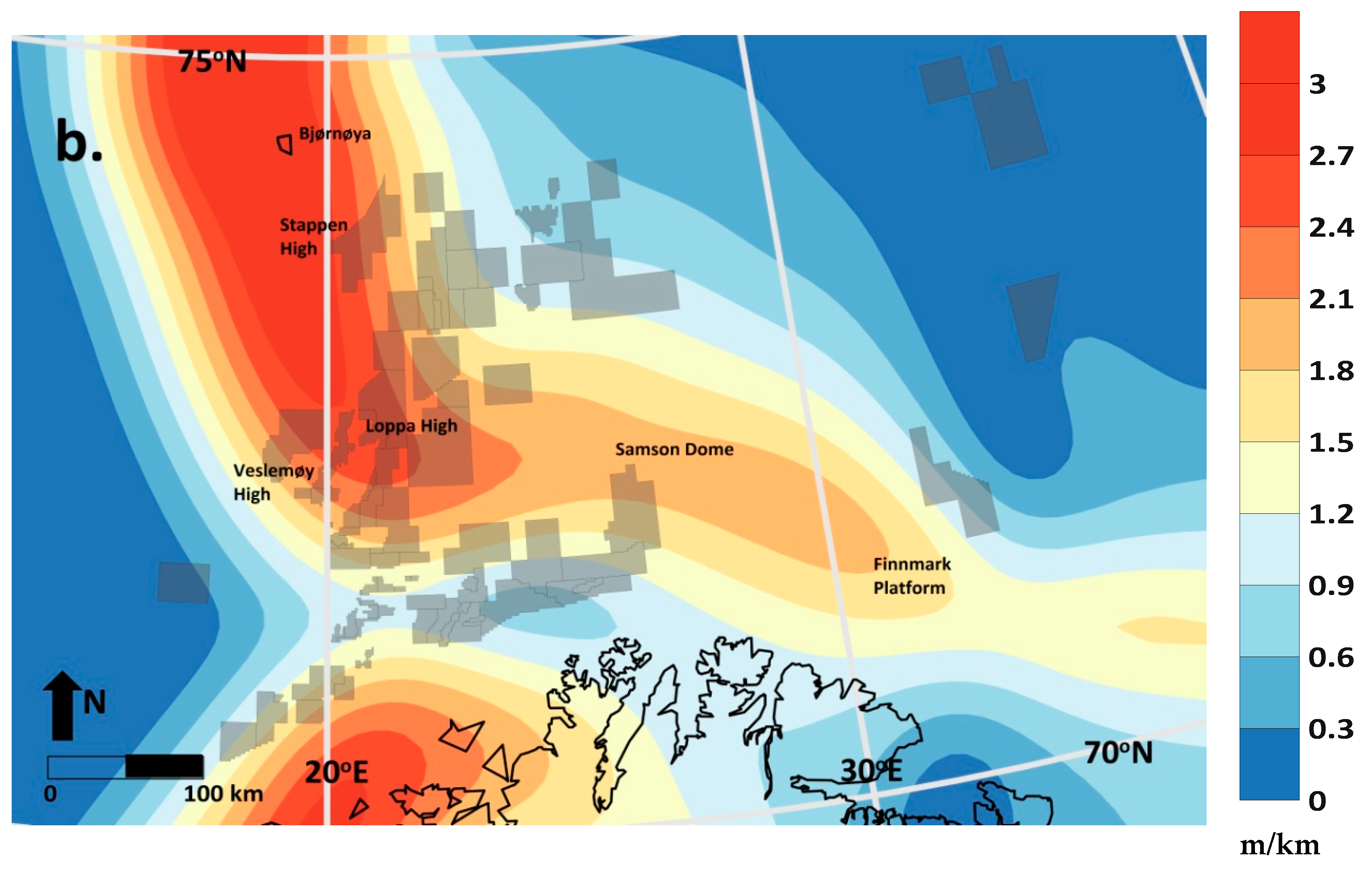
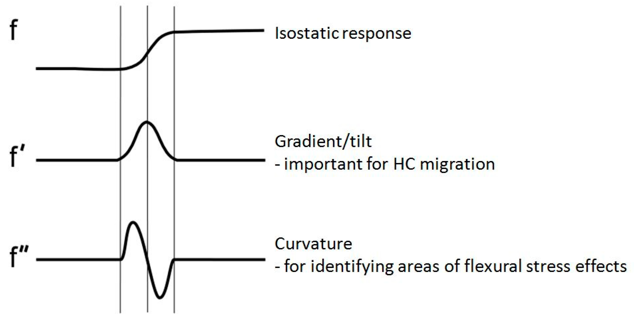
3.1. Identification of Glacially Flexured Areas
3.2. Model Setup
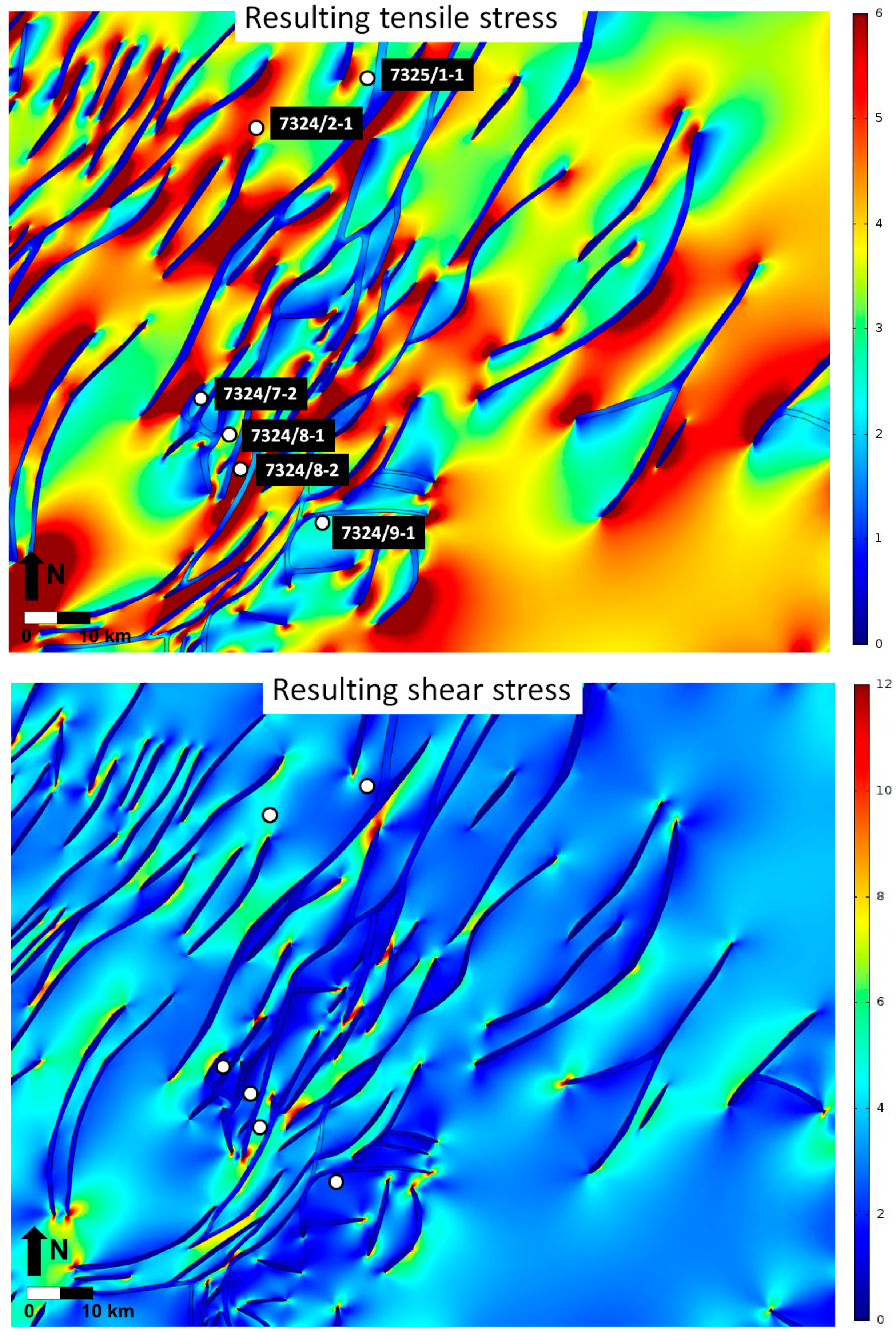
3.3. Results
4. Discussion
4.1. Glaciation Model
4.2. Earth Model
4.3. Stress Models
4.4. Implications for Basin Modeling
Author Contributions
Funding
Acknowledgments
Conflicts of Interest
Appendix A
Glacial Isostatic Model
References
- Gibbard, P.L.; Head, M.J.; Walker, M.J.C. Formal ratification of the quaternary system/period and the pleistocene series/Epoch with a base at 2.58 Ma. J. Quat. Sci. 2009, 25, 96–102. [Google Scholar] [CrossRef]
- Mangerud, J.; Gyllencreutz, R.; Lohne, Ø.; Svendsen, J.I. Glacial history of Norway. In Developments in Quaternary Science; Ehlers, J., Gibbard, P.L., Hughes, P.D., Eds.; Elsevier: Amsterdam, The Netherlands, 2011; Volume 15, pp. 279–298. ISBN 978-0-444-53447-7. [Google Scholar]
- Fjeldskaar, W.; Amantov, A. Effects of glaciations on sedimentary basins. J. Geodyn. 2018, 118, 66–81. [Google Scholar] [CrossRef]
- Argus, D.F.; Drummond, R.; Peltier, W.R. Space geodesy constrains ice age terminal deglaciation: The global ICE-6G_C (VM5a) model. J. Geophys. Res. Solid Earth 2015, 120, 450–487. [Google Scholar] [CrossRef]
- Kjemperud, A.; Fjeldskaar, W. Pleistocene glacial isostasy-implications for petroleum geology. In Structural and Tectonic Modelling and its Application to Petroleum Geology; Larsen, R.M., Brekke, H., Larsen, B.T., Talleraas, E., Eds.; Elsevier: Amsterdam, The Netherlands, 1992; pp. 187–195. [Google Scholar]
- Grunnaleite, I.; Fjeldskaar, W.; Wilson, J.; Faleide, J.; Zweigel, J. Effect of local variations of vertical and horizontal stresses on the Cenozoic structuring of the mid-Norwegian shelf. Tectonophysics 2009, 470, 267–283. [Google Scholar] [CrossRef]
- Vadakkepuliyambatta, S.; Bünz, S.; Mienert, J.; Chand, S. Distribution of subsurface fluid-flow systems in the SW Barents Sea. Mar. Pet. Geol. 2013, 43, 208–221. [Google Scholar] [CrossRef]
- Cavanagh, A.J.; Di Primio, R.; Scheck-Wenderoth, M.; Horsfield, B. Severity and timing of Cenozoic exhumation in the southwestern Barents Sea. J. Geol. Soc. 2006, 163, 761–774. [Google Scholar] [CrossRef]
- Doré, A.G.; Jensen, L.N. The impact of late Cenozoic uplift and erosion on hydrocarbon exploration: offshore Norway and some other uplifted basins. Glob. Planet. Change 1996, 12, 415–436. [Google Scholar] [CrossRef]
- Duran, E.R.; Di Primio, R.; Anka, Z.; Stoddart, D.; Horsfield, B. 3D-basin modelling of the Hammerfest Basin (southwestern Barents Sea): A quantitative assessment of petroleum generation, migration and leakage. Mar. Pet. Geol. 2013, 45, 281–303. [Google Scholar] [CrossRef]
- Zieba, K.J.; Grøver, A. Isostatic response to glacial erosion, deposition and ice loading. Impact on hydrocarbon traps of the southwestern Barents Sea. Mar. Pet. Geol. 2016, 78, 168–183. [Google Scholar] [CrossRef]
- Lerche, I.; Yu, Z.; Tørudbakken, B.; Thomsen, R. Ice loading effects in sedimentary basins with reference to the Barents sea. Mar. Pet. Geol. 1997, 14, 277–338. [Google Scholar] [CrossRef]
- Stoddart, D.; Jørstad, A.; Rønnevik, H.-C.; Fjeldskaar, W.; Løtveit, I.F. Recent glacial events in the Norwegian North Sea-implications towards a better understanding of charging/leakage of oil fields and its impact oil exploration. In Proceedings of the IMOG 2015—27th International Meeting on Organic Geochemistry, Prague, Czech Republic, 13–18 September 2015. [Google Scholar] [CrossRef]
- Medvedev, S.; Hartz, E.H.; Schmid, D.W.; Zakariassen, E.; Varhaug, P. Influence of Glaciations on North Sea Petroleum Systems; Geological Society: London, UK, Special Publications; 2019; Volume 494, p. SP494-2018-2183. [Google Scholar] [CrossRef]
- Mikko, H.; Smith, C.A.; Lund, B.; Ask, M.V.; Munier, R. LiDAR-derived inventory of post-glacial fault scarps in Sweden. GFF 2015, 137, 334–338. [Google Scholar] [CrossRef]
- Dehls, J.F.; Olesen, O.; Olsen, L.; Blikra, L.H. Neotectonic faulting in northern Norway; the Stuoragurra and Nordmannvikdalen postglacial faults. Quat. Sci. Rev. 2000, 19, 1447–1460. [Google Scholar] [CrossRef]
- Lagerbäck, R. Neotectonic structures in northern Sweden. Geol. Foren. Stockh. Förh. 1979, 100, 271–278. [Google Scholar] [CrossRef]
- Brandes, C.; Winsemann, J.; Roskosch, J.; Meinsen, J.; Tanner, D.C.; Frechen, M.; Steffen, H.; Wu, P. Activity along the Osning Thrust in Central Europe during the Lateglacial: Ice-sheet and lithosphere interactions. Quat. Sci. Rev. 2012, 38, 49–62. [Google Scholar] [CrossRef]
- Sandersen, P.B.E.; Jørgensen, F. Neotectonic deformation of a Late Weichselian outwash plain by deglaciation-induced fault reactivation of a deep-seated graben structure. Boreas 2015, 44, 413–431. [Google Scholar] [CrossRef]
- Grube, A. Palaeoseismic structures in Quaternary sediments, related to an assumed fault zone north of the Permian Peissen-Gnutz salt structure (NW Germany)—Neotectonic activity and earthquakes from the Saalian to the Holocene. Geomorphology 2019, 328, 15–27. [Google Scholar] [CrossRef]
- Hoffmann, G.; Reicherter, K. Soft-sediment deformation of late Pleistocene sediments along the southwestern coast of the Baltic Sea. Intern. J. Earth Sci. 2012, 101, 351–363. [Google Scholar] [CrossRef]
- Van Loon, A. (Tom); Pisarska-Jamroży, M. Sedimentological evidence of Pleistocene earthquakes in NW Poland induced by glacio-isostatic rebound. Sediment. Geol. 2014, 300, 1–10. [Google Scholar] [CrossRef]
- Stewart, I.S.; Firth, C.R.; Rust, D.J.; Collins, P.E.; Firth, J.A. Postglacial fault movement and palaeoseismicity in western Scotland: A reappraisal of the Kinloch Hourn fault, Kintail. J. Seism. 2001, 5, 307–328. [Google Scholar] [CrossRef]
- Fejerskov, M.; Lindholm, C. Crustal stress in and around Norway: an evaluation of stress-generating mechanisms. Geol. Soc. London Spéc. Publ. 2000, 167, 451–467. [Google Scholar] [CrossRef]
- Druzhinina, O.; Bitinas, A.; Molodkov, A.; Kolesnik, T. Palaeoseismic deformations in the Eastern Baltic region (Kaliningrad District of Russia). Estonian J. Earth Sci. 2017, 66, 119–129. [Google Scholar] [CrossRef]
- Antonovskaya, G.; Konechnaya, Y.; Kremenetskaya, E.O.; Asming, V.; Kvaerna, T.; Schweitzer, J.; Ringdal, F. Enhanced earthquake monitoring in the European Arctic. Polar Sci. 2015, 9, 158–167. [Google Scholar] [CrossRef]
- Gibbons, S.J.; Antonovskaya, G.; Asming, V.; Konechnaya, Y.V.; Kremenetskaya, E.; Kværna, T.; Schweitzer, J.; Vaganova, N.V. The 11 October 2010 Novaya Zemlya Earthquake: Implications for Velocity Models and Regional Event Location. Bull. Seismol. Soc. Am. 2016, 106, 1470–1481. [Google Scholar] [CrossRef]
- Neuzil, C.E. Hydromechanical effects of continental glaciation on groundwater systems. Geofluids 2012, 12, 22–37. [Google Scholar] [CrossRef]
- Steffen, R.; Steffen, H.; Wu, P.; Eaton, D.W. Reply to comment by Hampel et al. on “Stress and fault parameters affecting fault slip magnitude and activation time during a glacial cycle.”. Tectonics 2015, 34, 2359–2366. [Google Scholar]
- Grollimund, B.; Zoback, M.D. Post glacial lithospheric flexure and induced stresses and pore pressure changes in the northern North Sea. Tectonophysics 2000, 327, 61–81. [Google Scholar] [CrossRef]
- Johnston, A.C. Suppression of earthquakes by large continental ice sheets. Nature 1987, 330, 467–469. [Google Scholar] [CrossRef]
- Turpeinen, H.; Hampel, A.; Karow, T.; Maniatis, G. Effect of ice sheet growth and melting on the slip evolution of thrust faults. Earth Planet. Sci. Lett. 2008, 269, 230–241. [Google Scholar] [CrossRef]
- Steffen, R.; Steffen, H.; Wu, P.; Eaton, D.W. Stress and fault parameters affecting fault slip magnitude and activation time during a glacial cycle. Tectonics 2014, 33, 1461–1476. [Google Scholar] [CrossRef]
- Fjeldskaar, W.; Amantov, A. Tilted Norwegian post-glacial shorelines require a low viscosity asthenosphere and a weak lithosphere. Reg. Geol. Metallogeny 2017, 70, 48–59. [Google Scholar]
- Larsen, E.; Fredin, O.; Lyså, A.; Amantov, A.; Fjeldskaar, W.; Ottesen, D. Causes of time-transgressive glacial maxima positions of the last Scandinavian Ice Sheet. Nor. J. Geol. 2016, 96. [Google Scholar]
- Hughes, A.L.C.; Gyllencreutz, R.; Lohne, Ø.S.; Mangerud, J.; Svendsen, J.I. The last Eurasian ice sheets—A chronological database and time-slice reconstruction, DATED-1. Boreas 2016, 45, 1–45. [Google Scholar] [CrossRef]
- Zweck, C.; Huybrechts, P. Modeling of the northern hemisphere ice sheets during the last glacial cycle and glaciological sensitivity. J. Geophys. Res. Space Phys. 2005, 110, 1984–2012. [Google Scholar] [CrossRef]
- Auriac, A.; Whitehouse, P.L.; Bentley, M.J. Glacial isostatic adjustment associated with the Barents Sea ice sheet: A modeling inter-comparison. Quat. Sci. Rev. 2016, 147, 122–135. [Google Scholar] [CrossRef]
- Steffen, H.; Wu, P. Glacial isostatic adjustment in Fennoscandia—A review of data and modeling. J. Geodyn. 2011, 52, 169–204. [Google Scholar] [CrossRef]
- Amantov, A.; Fjeldskaar, W. Meso-Cenozoic exhumation and relevant isostatic process: The Barents and Kara shelves. J. Geodyn. 2018, 118, 118–139. [Google Scholar] [CrossRef]
- Fjeldskaar, W. The flexural rigidity of Fennoscandia inferred from the post-glacial uplift. Tectonics 1997, 16, 596–608. [Google Scholar] [CrossRef]
- Stephansson, O. Stress Measurements And Modelling of Crustal Rock Mechanics in Fennoscandia; In Earthquakes at North-Atlantic Passive Margins: Neotectonics and Postglacial, Rebound, Gregersen, S., Basham, P.W., Eds.; Springer: Dordrecht, The Netherlands, 1989; pp. 213–229. [Google Scholar]
- Stein, S.; Cloetingh, S.; Sleep, N.H.; Wortel, R.; Gregersen, S.; Basham, P.W. Passive Margin Earthquakes, Stresses and Rheology. In Earthquakes at North-Atlantic Passive Margins: Neotectonics and Postglacial Rebound; Springer: Dordrecht, The Netherlands, 1989; pp. 231–259. [Google Scholar]
- Cathles, L.M. The Viscosity of the Earth´s Mantle; Princeton University Press: Princeton, NJ, USA, 1975; p. 386. [Google Scholar]
- Brekke, H.; Kalheim, J.E.; Riis, F.; Egeland, B.; Blystad, P.; Johnsen, S.; Ragnhildstveit, J. Two-Way Time-Map of the Unconformity at the Base of Top Jurassic (North of 69° N) and the Unconformity at the Base of Cretaceous (South of 69°N), Offshore Norway, Including the Main Geological Trends Onshore. NPD Continental Shelf Map No. 1; The Norwegian Petroleum Directorate/The Geological Survey of Norway: Stavanger/Trondheim, Norway, 1992. [Google Scholar]
- Gudmundsson, A. Rock Fractures in Geological Processes, 1st ed.; Cambridge University Press: New York, NY, USA, 2011. [Google Scholar]
- Gudmundsson, A.; Simmenes, T.H.; Larsen, B.; Philipp, S.L. Effects of internal structure and local stresses on fracture propagation, deflection, and arrest in fault zones. J. Struct. Geol. 2009, 32, 1643–1655. [Google Scholar] [CrossRef]
- Paterson, M.S.; Paterson, D.M.S. Experimental Rock Deformation—The Brittle Field; Springer: Berlin, Germany, 1978; Volume 13. [Google Scholar]
- Farmer, I. Engineering Behaviour of Rocks; Chapman and Hal: London, UK, 1983. [Google Scholar]
- Amadei, B.; Stephansson, O. Rock Stress and its Measurement; Chapman and Hall: London, UK, 1997; p. 490. [Google Scholar]
- Jaeger, J.C.; Cook, N.G.W.; Zimmerman, R.W. Fundamentals of Rock Mechanics, 2nd ed.; Chapman and Hall: London, UK, 2007. [Google Scholar]
- Fjeldskaar, W.; Bondevik, S.; Amantov, A. Glaciers on Svalbard survived the Holocene thermal optimum. Quat. Sci. Rev. 2018, 199, 18–29. [Google Scholar] [CrossRef]
- Fjeldskaar, W.; Bondevik, S. The Early-Mid-Holocene transgression (Tapes) at the Norwegian coast–comparing observations with numerical modelling. Quat. Sci. Rev. (submitted).
- Medvedev, S.; Hartz, E.H.; Faleide, J.I. Erosion-driven vertical motions of the circum Arctic: Comparative analysis of modern topography. J. Geodyn. 2018, 119, 62–81. [Google Scholar] [CrossRef]
- Fjeldskaar, W.; Cathles, L. Rheology of Mantle and Lithosphere Inferred from Post-Glacial Uplift in Fennoscandia. In Glacial Isostasy, Sea-Level and Mantle Rheology; Springer: Berlin, Germany, 1991; pp. 1–19. [Google Scholar]


© 2019 by the authors. Licensee MDPI, Basel, Switzerland. This article is an open access article distributed under the terms and conditions of the Creative Commons Attribution (CC BY) license (http://creativecommons.org/licenses/by/4.0/).
Share and Cite
Løtveit, I.F.; Fjeldskaar, W.; Sydnes, M. Tilting and Flexural Stresses in Basins Due to Glaciations—An Example from the Barents Sea. Geosciences 2019, 9, 474. https://doi.org/10.3390/geosciences9110474
Løtveit IF, Fjeldskaar W, Sydnes M. Tilting and Flexural Stresses in Basins Due to Glaciations—An Example from the Barents Sea. Geosciences. 2019; 9(11):474. https://doi.org/10.3390/geosciences9110474
Chicago/Turabian StyleLøtveit, Ingrid F., Willy Fjeldskaar, and Magnhild Sydnes. 2019. "Tilting and Flexural Stresses in Basins Due to Glaciations—An Example from the Barents Sea" Geosciences 9, no. 11: 474. https://doi.org/10.3390/geosciences9110474
APA StyleLøtveit, I. F., Fjeldskaar, W., & Sydnes, M. (2019). Tilting and Flexural Stresses in Basins Due to Glaciations—An Example from the Barents Sea. Geosciences, 9(11), 474. https://doi.org/10.3390/geosciences9110474