Multiscale Modeling of Glacial Loading by a 3D Thermo-Hydro-Mechanical Approach Including Erosion and Isostasy

Abstract

We present a computational framework that allows investigating the Thermo-Hydro- Mechanical response of a representative part of a sedimentary basin during a glaciation cycle. We tackle the complexity of the problem, arising by the mutual interaction among several phenomena, by means of a multi-physics, multi-scale model with respect to both space and time. Our contribution addresses both the generation of the computational grid and the algorithm for the numerical solution of the problem. In particular we present a multi-scale approach accounting for the global deformation field of the lithosphere coupled with the Thermo-Hydro-Mechanical feedback of the ice load on a representative part of the domain at a finer scale. In the fine scale model we also include the erosion possibly caused by the ice melting. This methodology allows investigating the evolution of the sedimentary basin as a response to glaciation cycle at a fine scale, taking also into account the large spatial scale movement of the lithosphere due to isostasy. The numerical experiments are based on the analysis of simple scenario, and show the emergence of effects due to the multi-physics nature of the problem that are barely captured by simpler approaches.

1. Introduction

Reconstructing the stress and deformation history of a sedimentary basin is a challenging and important problem in the geosciences and a variety of applications [1]. The mechanical response of a sedimentary basin is the consequence of complex multi-physics processes involving mechanical, geochemical, geophysical, geological and thermal aspects [2]. The strongly coupled nature of the deformation problem may be understood in terms of the feedbacks underlying crustal dynamics. The pore fluid pressure affects stress, stress changes can lead to fracturing, and fracturing can affect pore fluid pressure [3,4].

Basin scale compaction processes involve mechanical and chemically induced transformations that take place during the accumulation of sediments [2]. In this context a number of approaches have considered the geochemical and mechanical compaction problem from a one-dimensional perspective, i.e., by considering mass, momentum and energy balances along the vertical direction, applied to fluid and solid phases [3,4,5,6]. These simplified one-dimensional approaches may be effective in interpreting qualitatively well data (e.g., [7]), however, they cannot capture inherently three dimensional processes that may arise due to the coupling of mechanical deformations and fluid mechanics in geological bodies that play an important role in the presence of glaciations [8].

Hydro-mechanical effects of continental ice sheets are widely recognized to cause movements and stresses of overridden terrains by ice load. The effect of the ice load on top of the sedimentary basin can be represented by the combination of two effects. The first is a large scale effect where we consider the action of the ice load on the entire lithosphere. The second is a fine scale analysis where we take into account the thermo-hydro-mechano-chemical (THMC) effects of the ice load into a small portion of the crust, such as a sedimentary basin [8].

In the global large scale framework, the interaction between the lithosphere and the glaciation cycle is modeled by means of a viscoelastic model. This choice is based on significant previous efforts devoted to define a proper mathematical model for the description of glacial isostatic adjustment. Initially this problem has been considered by Rayleigh [9] which studied the problem of a pre-stressed elastic compressible layer as an approximation of a “flat” planet. After Rayleigh’s work other authors enriched his theory, including many other details, like the effect of viscosity or the stratified structure of the Earth. First of all, Love [10] gave a more detailed theory and defined the basic concepts which are included in more recent works. Peltier and his coauthors in a series of articles [11,12,13] gave a detailed description of a more realistic viscoelastic model of stratified Earth. The Peltier’s model is essentially an extension of Love’s model, where a viscoelastic rheology is used instead of an elastic one. All the mathematical details of this theory are contained in the works of Biot and, more recently, Ogden [14,15].

In this work we apply these models to describe the global deformation field of the lithosphere and to extract from it the information of the movement of a selected part of the sedimentary basin. Since the spatial scale of such region is very small compared to the global scale, we describe it as a rigid motion. More precisely, the rigid motion of the fine scale basin model is extrapolated from the lithosphere displacement fields and used at run time to move the computational grid in the simulations. In what follows we describe in more details this the workflow of this multiscale approach.

A number of numerical simulation tools have been presented to model THMC processes [16,17,18]. While considering a similar mathematical approach, our work introduces the following new features with respect to previous studies:

(i)

it combines the global deformation of the lithosphere with the local simulation of pressure and temperature fields;

(ii)

it is built on available geophysical and geological information on the whole sedimentary system and relying on information available at selected wells;

(iii)

it allows considering the effects of erosion induced by glaciation, which is often neglected in previous studies.

Our work focuses on the integration of THM simulation of a single glaciation cycle with larger scale information available on basin scale compaction and lithosphere dynamics, thus the proposed THM simulation of glaciations can be cast within a multi-scale geological simulation framework. A visual sketch of the multiscale model outline is provided in Figure 1.

2. Isostatic Glacial Rebound Model

From the mechanical point of view the interior of the Earth can be considered as composed of four main layers: the inner and outer core, the mantle and the lithosphere [19]. During the growth of a continental ice sheet, the lithosphere under the ice load is deformed into the mantle and the removal of the ice load during deglaciation initiates a rebound process. The uplift is well known in formerly glaciated areas, e.g., North America and Scandinavia, and in currently deglaciating areas, e.g., Alaska, Antarctica, and Greenland. Compared to water, the mantle viscosity is ${10}^{22}$–${10}^{25}$ times higher, therefore the uplifting will be slowed down and continue long time after the ice has gone. The entire process of subsidence during the glacial growth, followed by uplift during and after deglaciation, is referred to as glacial isostatic adjustment.

The glacial isostatic adjustment process is dependent on the viscosity structure of the mantle, as well as the elastic thickness of the lithosphere. Observations of this process can therefore be used to gain insight into these properties of the Earth and this is important for an understanding of the dynamics of the Earth’s interior.

A well established assumption for the computation of the solid Earth response to surface ice loads over glacial timescales is that the Earth can be considered as a viscoelastic body ([20]). In particular the lithosphere can be assumed to be elastic and the solid mantle beneath behaves as a viscous fluid.

A complete review of the state of the art concerning the modeling and simulation of the glacial rebound can be found in [21,22] whereas the importance of this phenomenon in the context of basin simulation is discussed in [23,24,25].

In the next section the physical model adopted for the simulation of the post-glacial rebound is presented; the details of the numerical method can be found in Appendix A.

A Viscoelastic Model for the Earth

In accordance with the previously cited works the Earth has been modeled has a linear viscoelastic spherical shell $\mathsf{\Omega }\subset {\mathbb{R}}^3$ since the dynamics due to the glacial isostatic adjustment does not involve the core of the planet. Following the approach presented in [26] we assume that the viscoelastic stress tensor is given $\sigma ={\sigma }^e-q$, where ${\sigma }^e$ is the elastic stress and tensor q is an internal variable used to model the effects of viscosity. Denoting with $\mathbf{u}$ the displacement field, the elastic stress tensor ${\sigma }^e$ is given by the sum of the deviatoric and the volumetric parts

$${\sigma }^e=2\mu e\left(\mathbf{u}\right)-pI,$$

where I denotes the identity matrix. The deviatoric part is the product between the shear modulus $\mu$ and the deviatoric strain $e\left(\mathbf{u}\right)$ defined as

$$e\left(\mathbf{u}\right)=\frac{1}{2}(\nabla \mathbf{u}+{\nabla \mathbf{u}}^t)-\frac{1}{3}(\nabla ·\mathbf{u})I.$$

The volumetric part depends on the pressure p which is defined by the equation

$$\nabla ·\mathbf{u}+\frac{3}{2\mu }\frac{1-2\nu }{1+\nu }p=0,$$

(1)

where $\nu$ is the Poisson ratio.

The internal variable q is defined by the evolution equation

$$\left\{\begin{array}{c}\dot{q}+{\displaystyle \frac{1}{\tau }}q={\displaystyle \frac{1}{\tau }}2\mu e\left(\mathbf{u}\right),\hfill \\ q\left(0\right)=0,\hfill \end{array}\right.$$

(2)

where $\dot{q}$ denotes the derivative of the quantity q with respect to time and $\tau$ is called relaxation time and it is related to the viscosity $\eta$ through the relation $\tau =\frac{\eta }{2\mu }$.

The Equation (2) can be rewritten in the integral form as:

$$q\left(t\right)={\int }_0^t\frac{1}{\tau }{e}^{-\frac{t-s}{\tau }}2\mu e\left(\mathbf{u}\left(s\right)\right)ds.$$

By means of the previous expressions the viscoelastic stress tensor $\sigma$ is evaluated through a convolution integral defined as

$$\sigma \left(t\right)=-pI+{\int }_0^t{e}^{-\frac{t-s}{\tau }}2\mu e\left(\dot{\mathbf{u}}\left(s\right)\right)ds.$$

This equation coupled with the Equation (1) and with the equation of conservation of linear momentum give us a system of partial differential equations that describe the motion of a viscoelastic body:

$$\left\{\begin{array}{cc}\nabla ·\sigma +\mathbf{f}=0\hfill & \mathrm{in}\mathsf{\Omega },\hfill \\ \nabla ·\mathbf{u}+{\displaystyle \frac{3}{2\mu }}{\displaystyle \frac{1-2\nu }{1+\nu }}p=0\hfill & \mathrm{in}\mathsf{\Omega },\hfill \\ {\displaystyle \sigma =-pI+{\int }_0^t{e}^{-\frac{t-s}{\tau }}2\mu e\left(\dot{\mathbf{u}}\left(s\right)\right)ds}\hfill & \mathrm{in}\mathsf{\Omega }.\hfill \end{array}\right.$$

(3)

The unknowns of this system of equations are the displacement field $\mathbf{u}$, the pressure field p and the stress tensor field $\sigma$. The volumetric force field $\mathbf{f}$ is the gravitational force field, how this term has been modeled will be discussed later.

Since our domain is a spherical shell its boundary is the union of two connected components: the inner and the outer surfaces of the shell. The outer surface ${\mathsf{\Gamma }}_{\mathrm{out}}$ is the surface of the Earth and on this portion of the boundary we assume to know the history of the load due to the presence of the ice or other type of loads, like sediments. According to these data the following boundary condition is assumed: $\sigma \mathbf{n}={\mathbf{s}}_{\mathrm{load}}$ on ${\mathsf{\Gamma }}_{\mathrm{out}}$, where $\mathbf{n}$ denotes the outer normal defined on the boundary. The inner surface ${\mathsf{\Gamma }}_{\mathrm{in}}$ of the shell is chosen in such a way it corresponds to the core-mantle boundary (about 2900 $\mathrm{k}$$\mathrm{m}$ of depth). On this portion of the boundary the displacement $\mathbf{u}$ is assumed to be equal to zero, since the deformation due to the glacial isostatic adjustment involves only the shallow part of the mantle, until few hundreds of kilometer, namely $\mathbf{u}=0$ on ${\mathsf{\Gamma }}_{\mathrm{in}}$.

The force field $\mathbf{f}$ is given by the product between the density field $\rho$ and the acceleration gravity $\mathbf{g}$. Since we are dealing with a model of the whole Earth we cannot assume a constant value for the gravity and its value must be computed in accordance with the density field using the Gauss’s law for the gravity

$$\left\{\begin{array}{c}\mathbf{g}=-\nabla \varphi ,\hfill \\ \nabla ·\mathbf{g}+4\pi G\rho =0,\hfill \end{array}\right.$$

(4)

where G is the universal gravitational constant and the boundary conditions are $\mathbf{g}=-g_{\mathrm{surface}}\mathbf{n}$ on ${\mathsf{\Gamma }}_{\mathrm{out}}$ and $\varphi =0$ on ${\mathsf{\Gamma }}_{\mathrm{in}}$. Even though the displacement $\mathbf{u}$ is small if compared to the characteristic length of problem ( 1 $\mathrm{k}$$\mathrm{m}$ vs. 6371 $\mathrm{k}$$\mathrm{m}$) the gravity acceleration acting on the point change in accordance with the displacement field, so the force field $\mathbf{f}$ is given by $\rho \mathbf{g}(\mathbf{x}+\mathbf{u})\approx \rho \mathbf{g}\left(\mathbf{x}\right)+\rho \left({\nabla }_{\mathbf{x}}\mathbf{g}\right)\mathbf{u}$. From a physical point of view the first term $\rho \mathbf{g}\left(\mathbf{x}\right)$ is a static component, it does not change in time, on the other side the second term $\rho \left({\nabla }_{\mathbf{x}}\mathbf{g}\right)\mathbf{u}$ is the buoyancy term that determine the uplift and subsidence processes. This physical interpretation can be justified from a mathematical point of view. Exploiting the linearity of the problem the stress tensor $\sigma$ is decomposed as a sum of two components: a static stress term ${\sigma }^0$ (which is not important for our purposes) and a dynamic term ${\sigma }^d$ which is the solution of Problem Equation (3) with $\mathbf{f}=\rho \left({\nabla }_{\mathbf{x}}\mathbf{g}\right)\mathbf{u}$ and the boundary conditions.

3. The Thermo-Hydro-Mechanical Model Including Erosion

In this section we focus the attention on the mathematical framework describing the mechanical and thermal evolution of the basin. First, we show how the basin model is built and how we basin tilting is extracted from the large scale isostasy model. Second, we use mathematical models to describe the thermal and mechanical evolution of the basin under the effect of a glaciation cycle. The combination of these models consist in the multiscale modeling of glacial loading illustrated in Figure 1.

In the next sections the THMC model is introduced; the details of the numerical method can be found in Appendix B.

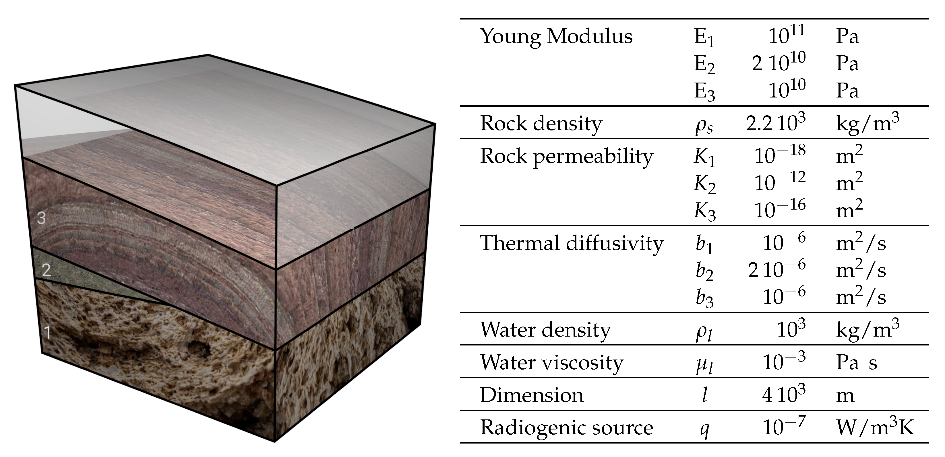
3.1. The Geological Model of a Sedimentary Basin

We assume that information about sedimentary units thicknesses, porosity and/or mineral composition are available at selected locations across a sedimentary system, typically from well logs, i.e., along the vertical direction (as sketched in Figure 1). In this framework we employ the stochastic inverse modelling procedure implemented in [7] to interpret vertical distributions of system properties with a one-dimensional model, which was developed in [5] starting from classical approaches to vertical compaction modeling (e.g., [2]). At each location such one-dimensional model provides an approximation of layers interface locations, whose characterization under uncertainty is investigated in detail in [27]. These interface locations can then be approximated in the whole domain starting from these data. This task is here performed using an interpolation based on ordinary kriging [28]. Our procedure assumes a smooth spatial variation of the sedimentary unit thicknesses. While this hypothesis can be restrictive in practical cases (e.g., in the presence of fault zones), our procedure is still able to handle geological settings of interest such as the occurrence of pinch out layers.

3.2. Extraction of the Basin Tilting From the Isostasy Model

The isostatic movement of the basin is taken into account as a rigid motion. In particular, we locate the computational cell that embed the fine scale geometrical model from the isostatic adjustment simulation, as shown in Figure 3. From the displacement field of the selected cell we evaluate the deformation gradient and the vertical rigid motion. We then isolate the rotational part of the deformation gradient that is uniquely defined by the polar decomposition [29], $F=R·U$, where F is the deformation gradient, U is the symmetric stretch tensor and R, such that $det\left(R\right)=1$, is the rotation matrix that we want to determine. In particular, from the deformation gradient we evaluate the Right Cauchy-Green Deformation Tensor namely matrix $G:=F^T·F$. Using the definition of F, we obtain that $G={\left(RU\right)}^T·\left(RU\right)=\left(U^T·R^T\right)·\left(R·U\right)$, and using the orthogonality of the rotation matrix, namely $R^T=R^{-1}$, we obtain $G=U^T·U$. We recall that U is a diagonalizable matrix so can be represented by $U=Q^{-1}·\mathsf{\Lambda }·Q$, where Q is the square matrix in which the ith column is the eigenvector $q_i$ of U and $\mathsf{\Lambda }$ is the diagonal matrix composed by the corresponding eigenvalues, namely ${\mathsf{\Lambda }}_{ii}={\zeta }_i$. We recall that U is a symmetric matrix so $U^T·U=U·U$, so using the spectral decomposition we obtain that $G=\left(Q^{-1}·{\mathsf{\Lambda }}^2·Q\right)$ where ${\mathsf{\Lambda }}^2$ is a diagonal matrix defined by ${\mathsf{\Lambda }}_{ii}^2={\zeta }_i^2$. From the previous considerations, it follows that by computing the eigenvalues and the eigenvectors of G, which is a known matrix, we calculate the matrix Q, ${\mathsf{\Lambda }}^2$, and, as a consequence, $\mathsf{\Lambda }$. Using $U=Q^{-1}·\mathsf{\Lambda }·Q$ we compute the matrix U so that we finally retrieve the rotation matrix R using $R=F·U^{-1}$.

The collection of the rotation matrices together with the axial displacement evaluated at every time step of the isostatic adjustment simulation, defines the rigid motion that we consider in fine scale model. In particular we use a Lagrangian and an Eulearian approach for the mechanical and the thermal problems, respectively. More precisely, in the mechanical problem the imposed rigid motion does not causes any additional stress so that the calculation of stress and the strain can be performed in the reference (static) configuration, while the rotation matrix is used to change the orientation of the gravity vector. In this framework, we let pressure, flow and displacement evolve under the action of the weight of the basin and of the ice. Concerning the thermal evolution of the basin we account of the variation of the heat flux with the isostatic movement of the sedimentary basin by means of the Eulerian approach, that is we actually move the domain in the computational model. In this way, both the vertical displacement and the rotation matrix are taken into account in the evaluation of the thermal source, as it will be discussed later.

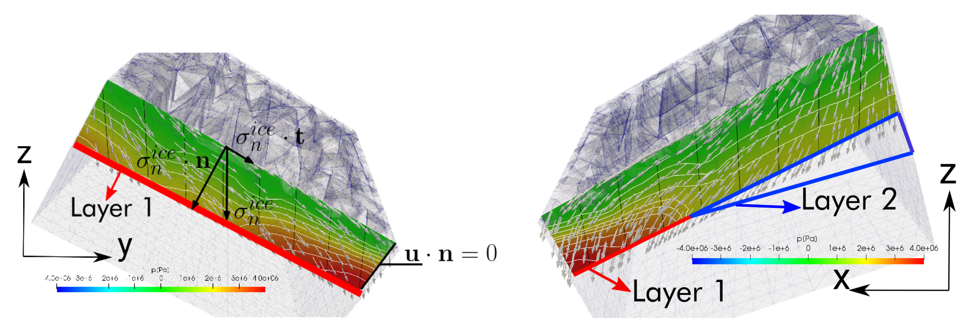
3.3. A Poromechanical Approach to Coupled Hydro-Mechanical Effects

For the mechanical evolution of the basin we rely on the theory of poroelasticity introduced by Biot in [30] under the quasi-static assumption for modeling a linearly elastic fully saturated porous medium. Such approach is widely used in literature, see [1,16,31,32] for a non exhaustive list of examples. Given a domain $\mathsf{\Omega }\in {\mathbb{R}}^d$, we consider for simplicity an isotropic material (named the skeleton) filled with an isothermal single-phase fluid. A sketch of a typical domain together with the frame of reference is shown in Figure A1. In this framework the momentum equation reads

$$\begin{array}{ccc}\hfill -\nabla ·\sigma \left(\mathbf{u}\right)+\alpha \nabla p& =\mathbf{f}\hfill & \hfill \mathrm{in}\mathsf{\Omega }\left(t\right),\end{array}$$

(5)

$$\begin{array}{ccc}\hfill {\partial }_t\left(\frac{p}{M}+\alpha \nabla ·\mathbf{u}\right)-\nabla ·K\nabla p& =0\hfill & \hfill \mathrm{in}\mathsf{\Omega }\left(t\right),\end{array}$$

(6)

where (with little abuse of notation with respect to the isostatic adjustment model) here $\mathbf{u}$ denotes the solid matrix displacement vector and p is the variation of pore pressure from the hydrostatic load. We notice that ${\partial }_t$ denotes the standard partial derivative with respect to time in the Eulerian framework. The parameters $\alpha$, M and K are the Biot coefficient, the Biot modulus and the hydraulic conductivity, respectively. We recall that the hydraulic conductivity is defined as the ratio between the permeability $k_s$ and the dynamic viscosity of the fluid ${\mu }_f$, namely $K=k_s/{\mu }_f$. Finally $\mathbf{f}$ is the gravity load of the porous material evaluated as $\mathbf{f}=({\rho }_s-{\rho }_f)\mathbf{g}$, where ${\rho }_s$, ${\rho }_f$ and $\mathbf{g}$ are the fluid density, the solid density and the gravity vector, respectively. We remark that in the mechanical model the isostasy movement coming from the isostatic adjustment simulation is taken into account by means of a Lagrangian approach. As a consequence, the gravity vector $\mathbf{g}$ varies during the simulation according to a prescribed profile. Such profile is defined by the angles evaluated from the polar decomposition of the deformation gradient of the computational cell, of the large scale simulation, that contains the portion of the sedimentary basin we consider. To complete the definition of the problem we recall the linear elasticity behavior for the skeleton. This implies that the stress tensor $\sigma$, appearing in (5), is defined by $\sigma \left(\mathbf{u}\right):=2\mu \epsilon \left(\mathbf{u}\right)+\lambda \nabla ·\mathbf{u},$ where $\mu$ and $\lambda$ are the Lamé coefficients and $\epsilon \left(\mathbf{u}\right)$ is the symmetric gradient of the skeleton displacement. For further details on poromechanical modeling, the interested reader is referred to e.g., [32,33].

For a well-posed problem we must complement the previous governing equations with appropriate boundary and initial conditions. Concerning the initial condition, the following constraints $\mathbf{u}=0$ and $p=0$ are considered at the initial time $t=t_0$. Let us label with $\mathsf{\Gamma }$ the top surface of the basin, while $\partial {\mathsf{\Omega }}_b$ and $\partial {\mathsf{\Omega }}_l$ are the bottom and the lateral boundary of the domain $\mathsf{\Omega }$, as show in Figure A1. According to this notation, we consider the following boundary conditions, $p=0,\sigma \left(\mathbf{u}\right)·\mathbf{n}={\sigma }_{ice}\left(t\right) \mathrm{on} \mathsf{\Gamma }\left(t\right),$ $\mathbf{u}=0,\nabla p·\mathbf{n}=0 \mathrm{on} \partial {\mathsf{\Omega }}_b\left(t\right),$ $\mathbf{u}·\mathbf{n}=0,\nabla p·\mathbf{n}=0 \mathrm{on} \partial {\mathsf{\Omega }}_l\left(t\right)$, where $\mathbf{n}$ is the unit outward normal to the boundary and ${\sigma }_{ice}\left(t\right)$ is the load resulting from the ice sheet on top of the basin. We further assume that the load relative to the solid component of the ice sheet transfers only to the solid matrix of the basin, while the fluid phase at the top surface is subject to the hydrostatic load.

3.4. Thermal Effects

The heat transfer is modeled through the following advection diffusion equation

$${\rho }_b{c}_b\frac{\partial T}{\partial t}+{\rho }_f{c}_f{\mathbf{v}}_D·\nabla T-\nabla ·(b\nabla T)=q_r,$$

(7)

where T is the temperature field, ${\rho }_f$ and $c_f$ are the fluid density and specific heat, respectively; ${\rho }_b$ and $c_b$ are the bulk density and the bulk specific heat defined as ${\rho }_b{c}_b=\varphi {\rho }_f{c}_f+(1-\varphi ){\rho }_s{c}_s$ with $\varphi$, ${\rho }_s$ and $c_s$ being the porosity, the solid density and specific heat capacity; ${\mathbf{v}}_D$ is the Darcy velocity defined as ${\mathbf{v}}_D=-K\nabla p$, b is the bulk thermal conductivity which is an average of the conductivity of the solid and the fluid phase and finally $q_r$ is the heat source. Concerning the initial condition, we consider an homogeneous temperature field, namely $T=0\forall \mathbf{x}\in \mathsf{\Omega }(t=t_0)$. According to the nomenclature shown in Figure A1, we consider the following boundary conditions, $T=T_{ice}\left(t\right) \mathrm{on} \mathsf{\Gamma }\left(t\right)$, $\nabla T·\mathbf{n}=0 \mathrm{on} \partial \mathsf{\Omega }\left(t\right)\backslash \mathsf{\Gamma }\left(t\right)$, where $\mathbf{n}$ is the unit outward normal to the boundary and $T_{ice}\left(t\right)$ is the basin top temperature. Following a widely used approach in literature, see for example [16,25], the presence of the ice on top of the basin is taken into account by means of a variation of the top temperature of the basin ($T_{ice}\left(t\right)$) during the glaciation cycle.

4. Results and Discussion

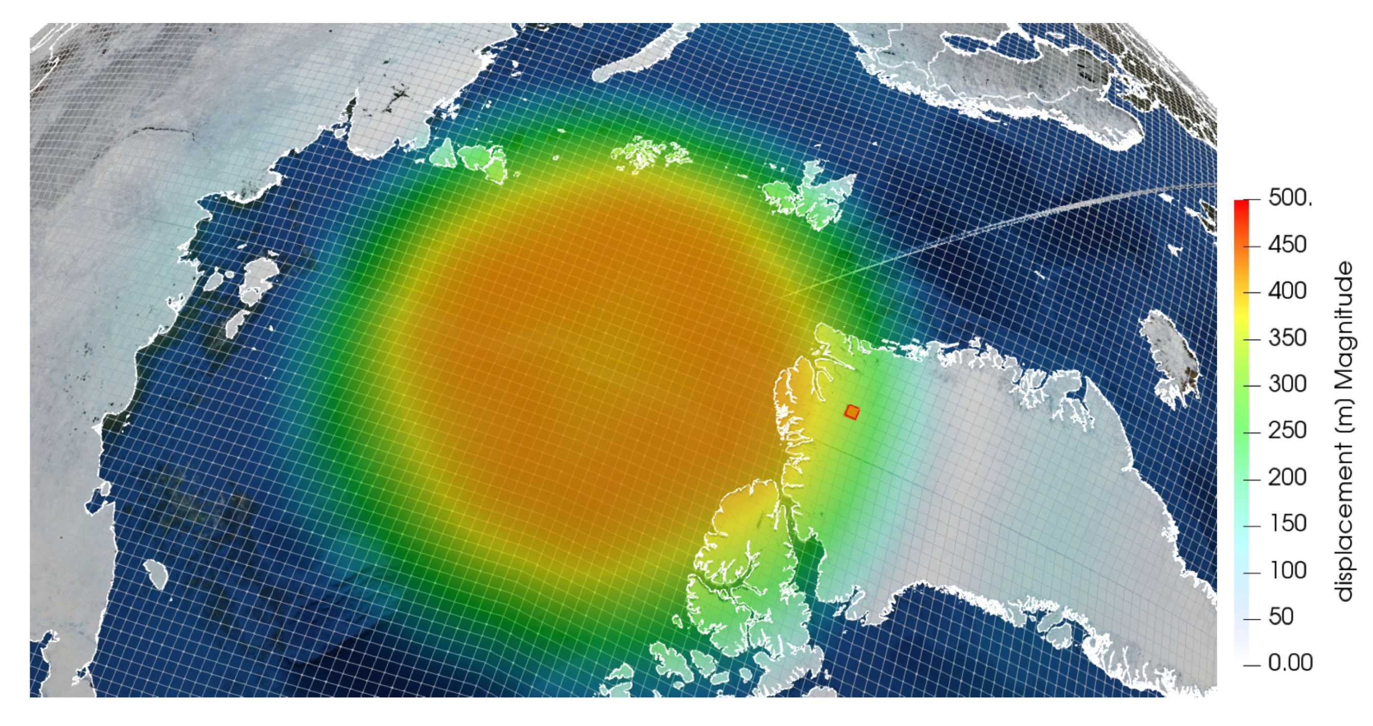
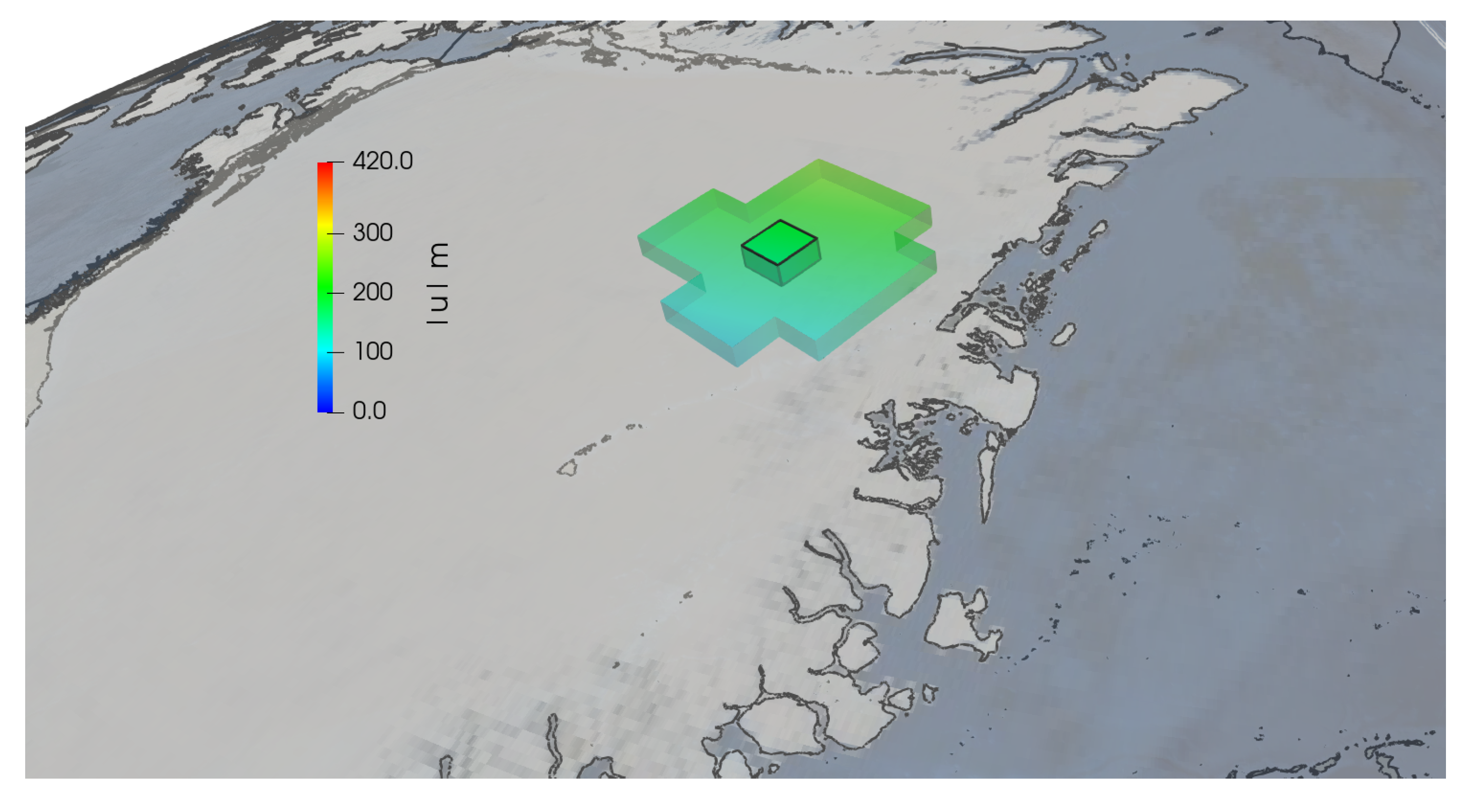
4.1. Results of the Glacial Rebound Model

The glacial rebound simulation addresses the deformation of the lithosphere of the whole Earth, based on a viscoelastic model. The forcing term of such simulation is the load of the ice sheet under a glaciation cycle.

The approach presented in this work is different from the one presented in the previously cited articles [11,12,13]. In these articles the authors describe a model for the deglaciation, the initial condition of their model is a glaciated Earth, the authors take into account the presence of this load at the initial condition defining a prestressed configuration. We rather simulate a full cycle of glaciation-deglaciation process to avoid the definition of a prestressed configuration, in our model the initial condition considered is a fully relaxed configuration, without enforced load.

In this case we consider a benchmark problem, where a circular sheet of radius $R=1111$ km (equivalent to an angular sector of ${10}^{\circ }$) centered at the North pole is formed and melt over a time window of 26 × 10${}^3$ years, according to the variable thickness profile shown in Figure 2. More precisely, we assume that the glaciation phase starts 26 × 10${}^3$ years ago and ends at present. We split this time window in three uniform intervals of 8.6 × 10${}^3$ years each. In the first one we assume formation of the ice sheet up to a maximal thickness of 4 km. In the central phase, we assume that the ice is static, while in the last term we model ice melting with a linearly decreasing profile of the ice thickness. The results of such simulation are reported in Figure 3. In Figure 4 we show a zoom of the computational cells on the crust layer of the glacial rebound simulations. The zoom is taken in correspondence of the computational cell used to calculate the deformation gradient F. More precisely, the numerical calculation of the deformation gradient involves the displacement field in the x, y and z direction at the nodal points of of the selected cell. The time history of the displacement at these time points is shown in Figure 5. Even if the presented test is just a synthetic example, the order of magnitude of the obtained vertical displacement is reasonable and in good agreement with the results reported in [24,25].

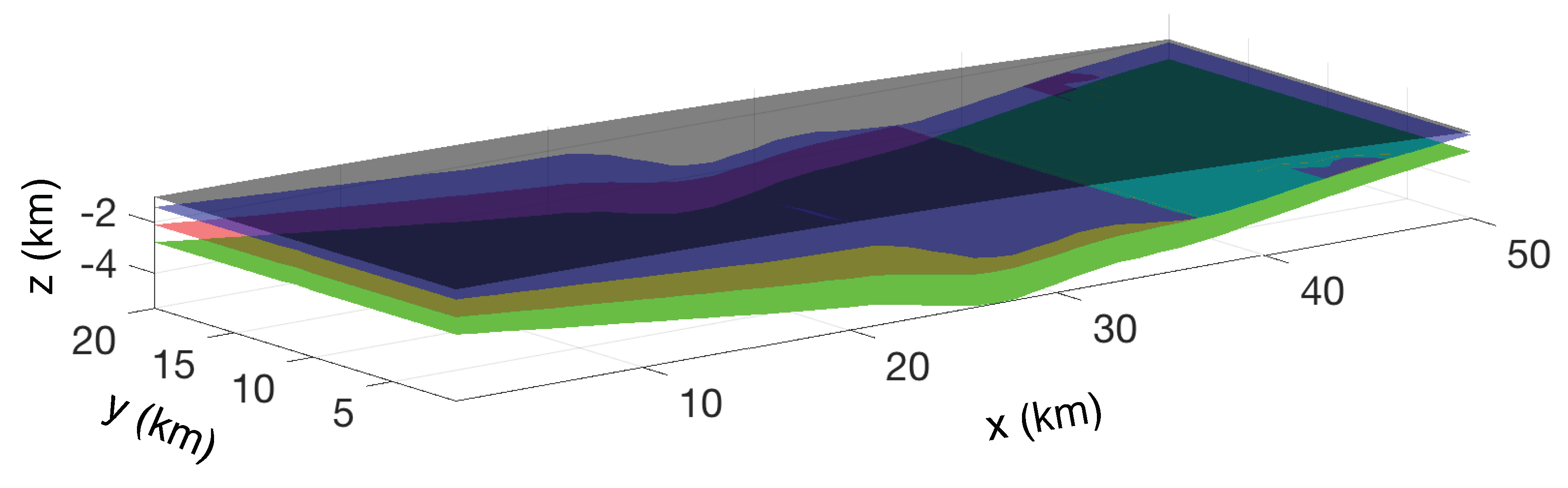
4.2. Results of the Kriging Algorithm for the Geological Basin Model Setup

An example of a simple reconstructed basin geometry is represented in Figure 6. These results are obtained on a synthetic example which considers a domain of 50 by 20 km in planar dimension. The one-dimensional simulations consider sediment deposition for a total period of time of 40 Ma. The sedimentation velocity is assumed to be fixed in time and is assigned at each $x,y$ location between a maximum value 90 m/Ma (at the domain center) and and a minimum of 40 m/Ma (at the domain boundaries, i.e., at $x=0$ and $x=50$ km). Interfaces between different layers are approximated in such a domain by applying ordinary kriging starting from interface depths calculated at 20 locations randomly placed in the computational domain. Four interfaces are considered in total, including the top and bottom surfaces. We assume that two interface collapse on each other, i.e., the second and third interface correspond for $x>35$ km. This means that one of the layers is not found at locations $x>35$ km, and that a layer pinch-out occurs.

Note that in the simulation approach presented in Section 3 the effects of chemical compaction processes, such as quartz precipitation and smectite to illite transformation [6,34,35], are not explicitly included. However, the effects of chemical processes are considered in the one-dimensional model employed to approximate the interfaces [5,36] at selected locations, and therefore are implicitly embedded in the system geometry. The geometrical reconstruction of the sedimentary system obtained in this way can then be further enriched by mapping mineral compositions, porosity, permeability or other properties which may be available at selected location, e.g., through compositional kriging. These data are not considered in the following for simplicity.

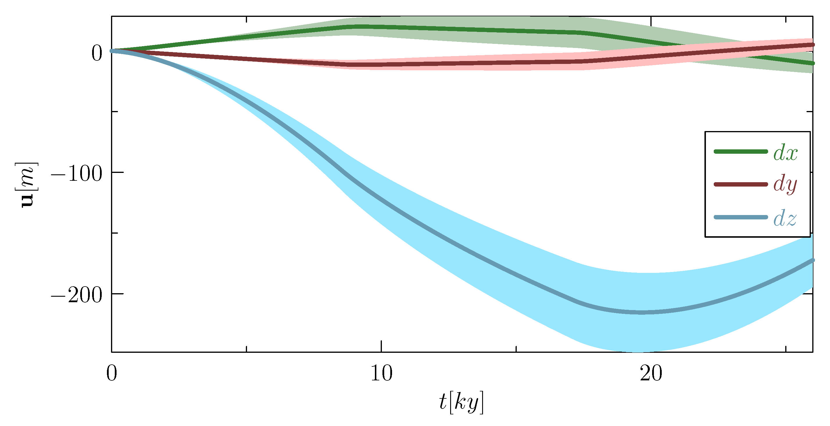
4.3. Results of the Thermo-Hydro-Mechanical Effects of Glaciation

In this section we consider the application of the solver described in Section 3. As introduced in Section 3.3, the mechanical effect of the glaciation is taken into account by means of a variable load. This load is related to the height of the ice accumulated on top of the basin and follows the curve shown in the left part of Figure 2. Concerning the thermal problem, adiabatic conditions are considered at the bottom and the lateral surfaces of the physical domain while a time-dependent temperature profile is imposed in the top boundary of the basin. This profile models the thermal effect of the ice and it is shown in the right panel of Figure 2.

The configuration of the basin simulated in this section and the physical parameters used to initialize the THM model are reported in Figure 7. More precisely, to perform the three-dimensional THM simulation, we consider a portion of the basin of $4\times 4$ km size with an average depth of of $2.8$ km located at the $x,y$ coordinates (32.5, 36.5) × (8, 12) km of the basin shown in Figure 6. The domain is split into three layers (numbered as 1,2 and 3 from bottom to top, as shown in the left part of Figure 7) and one of them is not continuous across the whole planar domain size resulting in a geological model with a pinch-out, consistent with the data in Figure 6. The material properties of all the different components of the basin are summarized in the right panel of Figure 7. We assume that the intermediate layer has a permeability that is significantly higher than the other ones and we consider the evolution of the basin during a time window of 26 ky with a time step of $0.14$ ky chosen to follow with enough detail glaciation evolution.

In the example of this section, the surface erosion on top of the basin is active during the last 8.7 ky of the simulation. It is modeled as the prescribed evolution of the upper part of the sedimentary basin. More precisely, we assume that during the last part of the simulation a certain amount of material is removed from the upper part of the basin. As a consequence the top surface of the physical domain evolves from $S_1$ to $S_2$, as shown in Figure 8. From the modeling standpoint, the motion of the top surface is described by means of a the level set function, that is defined in terms of spatial coordinates $x,y$ and time t,

$$\begin{array}{cc}\hfill & ls(x,z,t)=-(-0.285x+1.6z+12353)+400(1+a),\hfill \end{array}$$

(8)

$$\begin{array}{cc}\hfill & a=0\mathrm{if}t<-8.7Ky,\hfill \end{array}$$

(9)

$$\begin{array}{cc}\hfill & a=\frac{t+8.7Ky}{8.7ky}\mathrm{if}t\ge -8.7Ky.\hfill \end{array}$$

(10)

Finally, in the simulations presented in this section, we consider that the basin is exposed to a spatially dependent heat source $q_r$, determined by the heat flux from the mantle and by the internal radiogenic thermal source. The combination of these factors is accounted as a volumetric thermal source of this form $q_r\left(\mathbf{x}\right)=q_r\left(z\right)=q_{0}f\left(z\right)$. Following [37], the baseline source $q_0$ is determined by means of a heat balance equation that distributes over the basin volume the heat flux coming form the bottom surface (i.e., the one closer to the mantle) and the radiogenic source. Precisely, we set $q_0=\varphi S/V+q_{r,0}$ where $\varphi$ is the surface heat flux from the bottom surface, S, V is the basin volume and $q_{r,0}$ is the baseline radiogenic source. In this way we obtain $q_0=0.1$ $\mathsf{\mu }$W/m${}^3$. To account for the exponentially decreasing radioactivity with depth, this source is evaluated as a function of the actual position of the domain according to the following empirical formula $q=q_0{e}^{-z/D}$ where the parameter $D=5$ km.

The kriging-based horizon reconstruction addressed before approximates the interface locations on a user-defined spatially uniform grid (with uniform size equal to 0.5 km in our example), so that each interface is represented by a point cloud. Such point clouds are used to generate the internal surfaces of the basin as shown in the left panel of Figure 9. Then the boundaries of the horizons are used for the creation of the lateral surfaces of the geological model as shown in the middle panel. These operations result in the definition of a water tight geological model and are performed using the platform GOCAD. The geological model is then used as the input of the mesh generator RINGMesh [38] that produces the 3D a labeled computational grid shown in Figure 9, right panel.

For the analysis and the interpretation of the results we subdivide the simulation in three different phases: phase A (formation of the ice sheet) from $-26$ to $-17.4$ ky where the ice is growing, phase B (isostatic adjustment) from $-17.4$ to $-8.7$ ky where the ice load is steady and most of the isostatic motion takes place and the phase C (erosion) from $-8.7$ to 0 ky where the ice on top of the basin vanishes and the erosion takes place. A schematic of this temporal subdivision is reported in Figure 10. The current configuration of the domain $\mathsf{\Omega }\left(t\right)$, rotated according to the rigid motion coming from the isostatic adjustment simulation at different time steps, is shown in Figure 11.The evolution of displacement and pressure along the phases A, B and C of the simulation is shown in Figure 12. In the first phase (A), the action of the ice load generates the mechanical compaction of the basin. According to the Biot model the compaction leads to an increase in the pore pressure in the different layers of the basin. This effect is more evident in the top layers, 2 and 3, while layer 1 is almost unperturbed, because it is the most impermeable and it is subject to zero displacement conditions on the bottom surface. Moreover, we notice that the pressure field in the pinch out layer (layer 2) is almost uniform and equal to the value at the interface with the upper layer (layer 3). This effect is due to the fact that layer 2 is the most permeable. According to the Darcy law, this is the region where the smallest pressure gradients are observed.

In the second phase (B) we can observe the effect of the isostatic adjustment. The interaction between the isostatic motion end the poromechanical problem is illustrated in Figure 12 and Figure 13, where we show at $t_B=-13$ ky the pressure field in an internal slice of the domain, together with the displacement direction inside layer 3. We observe that the imposed rotation generates a tangential component of the load applied on the top of layer 3, namely ${\sigma }_n^{ice}·\mathbf{t}\ne 0$. This effect, combined with the boundary conditions enforcing zero normal displacement on the lateral surfaces of the basin, generates a mechanical compression effect along the tangential direction of the top and bottom surface planes of layer 3. Because of the poromechanic coupling, this tangent stress induces the pressure peak observed at the left corner of the basin. Furthermore, in the right part of Figure 13, an internal slice along the $xz$ plane is shown. From this view, the transition from layer 1 to layer 2 (at the pinch out) is visible. In this visualization, the effect of the permeability jump can be appreciated. More precisely, the pressure increases only along the interface between layers 1 and 3, while the pressure gradients are significantly smeared out along the contact line with layer 2 as a consequence of the high permeability of it. Finally, we notice that these effects are difficult to appreciate in the bottom layer, where the high young modulus limits the displacement field and the low permeability almost blocks the diffusion of the pressure peak occurring in the top layer.

To appreciate the impact of taking into account the isostatic response, we compare the pressure field in the top layer with the one obtained through a different numerical experiment in which we neglect the isostatic adjustment and the erosion. In the second scenario the basin model is completely static. In such case, because the load on top of the basin is constant, the general temporal trend of the pressure is to progressively reach a steady state in all the layers of the basin according to the characteristic temporal scale determined by the different permeability values.

The comparative study of the two scenarios described above is reported in Figure 14. In this Figure we compare the pressure field along two transversal lines $r_1$ and $r_2$, obtained switching on (first scenario, solid line) and off (second scenario, dashed line) the isostatic motion of the basin. As previously observed in the central panel of Figure 12, we notice that in the first scenario the pressure reaches a peak in the left corner of the layer 3 (as also illustrated in Figure 14). Such peak is not present in the second scenario, where we neglect the isostatic movement of the basin, as we can see from Figure 14 (dotted line). From that comparison we notice that limited spatial variations of the pressure are generate without taking into account the rigid motion of the basin, Conversely, the introduction of the isostatic rebound significantly increases the pressure variability, generating local peaks that depend on the morphology of the basin. Then, we conclude that the motion due to the isostatic adjustment simulation is the primary reason of the overpressure generation.

We now focus on the final phase (namely phase C) when the ice sheet is disappearing from the top of the basin and the erosion takes place. In this phase the mechanical load due to the ice weight goes to zero. The reduction of mechanical compaction is also augmented by the erosion of the top part of the basin. The combination of these effects leads to a general decrease of the pore pressure in all layers, as shown in the right panel of Figure 12, right column. More precisely, the lowest values of pressure (in terms of variations from the hydrostatic load) are located in the softest layer.

Concerning the temperature field, the model is initiated with a temperature field at thermal equilibrium and it evolves according to the (time dependent) heat equation under the action of a space dependent heat source. To analyze and validate the simulation of the thermal field we address two indicators: the overall thermal gradient from the top to the bottom of the basin and the temporal variations of the temperature from the steady state. Concerning the vertical temperature gradient, we observe from Figure 15 that a difference of $60 \mathrm{degC}$ along the vertical axis is established as a consequence of thermal balance between the thermal source and the imposed temperature at the top of the basin. This results is in good agreement with the thermal gradients expected in literature, see for example [37,39] for thermal properties and, in particular [37] for expected temperature profiles. For a more detailed analysis of the thermal variations from the initial equilibrium state, we report, in Figure 16, difference of the temperature field at time $t_A=-21.7ky$ $t_B=-13Ky$ from the one at $t_0=-26Ky$. We notice that at $t_A$ and $t_B$, the main temperature variations are driven by the increase of surface temperature from $-10 \mathrm{deg}C$ to $0 \mathrm{deg}C$ at the top of the basin, due to the protective effect of the ice cap, that is progressively forming in this phase. Comparing more in detail the profiles at $t_A$ and $t_B$, we observe that at time $t_B$ the temperature in the central part of the basin has slightly increased with respect to the one at $t_A$, by the effect of the thermal source. The profile at $t_C$ differs significantly form the others, because of the erosion, active in the time interval from $t_B$ to $t_C$. During erosion, the reference temperature of $0\mathrm{deg}C$ enforced at the contact interface with the ice, progressively shifts downwards, swiping a region of the basin that was previously hotter than $0\mathrm{deg}C$. For this reason, the temperature in the basin after erosion significantly decreases with respect to the initial time. Finally, in Figure 11 we report the variation of the total thermal source term, relative to the initial state, that is the spatial integral during the evolution of the domain $\mathsf{\Omega }\left(t\right)$ of the heat source ${\int }_{\mathsf{\Omega }\left(t\right)}q\left(\mathbf{x}\right)d\omega /{\int }_{\mathsf{\Omega }\left(t_0\right)}q\left(\mathbf{x}\right)d\omega$. These data suggest that variation of the basin volume due to erosion decreases the thermal source more significantly than the progressive increase of basin depth due to isostasy.

The analysis of the thermal field confirms that, in the short time window of one cycle of glaciation, the surface temperature, possibly modulated by erosion, is the main diving factor that determines temperature variations from the equilibrium state. This finding is in accordance with the detailed analysis of the effects of glaciations on sedimentary basins provided in [25]. It should also be observed that using a time dependent heat equation correctly models the natural inertia of the basin to change its equilibrium state. As a result, it is expected that the repetition of many glaciation cycles is required to significantly cool down the entire basin.

5. Conclusions

We have developed a fully coupled multiphysics and multiscale description of the evolution of a sedimentary basin under the effect of a glaciation cycle. To the best of our knowledge, thermo-hydro-mechanical effects are combined with isostatic adjustment and erosion within a fully time dependent three-dimensional simulation for the first time. Although the geological model that has been considered does not represent yet the complexity of a real sedimentary basin, we have described a pipeline of steps that could handle the most complex cases as well, thanks to a multiscale approach that decouples phenomena occurring at very different space and time scales. For example, our methodology establishes a quantitative framework to transfer information from the definition of a large scale geological architecture to local fluid displacement and deformation dynamics. Preliminary numerical results suggest that the combination of all these phenomena reveals the emergence of effects that were not expected or predictable using simpler approaches. In the considered synthetic test case we have quantified the effects of large scale isostatic displacement on local pressure and displacement field, in the presence of layer a pinch-out. Moreover, our results demonstrate the effect of erosion on the temperature dynamics of the sedimentary system. We believe that our results show the predictive potential of this holistic description of sedimentary basins subject to glaciations.

References

1. Tuncay, K.; Park, A.; Ortoleva, P. Sedimentary basin deformation: An incremental stress approach. Tectonophysics 2000, 323, 77–104. [Google Scholar] [CrossRef]
2. Wangen, M. Physical Principles of Sedimentary Basin Analysis; Cambridge University Press: Cambridge, UK, 2010. [Google Scholar]
3. Bethke, C. A numerical-model of compaction-driven groundwater-flow and heat-transfer and its application to the paleohydrology of intracratonic sedimentary basins. J. Geophys. Res. 1985, 90, 6817–6828. [Google Scholar] [CrossRef]
4. Tuncay, K.; Ortoleva, P. Quantitative basin modeling: Present state and future developments towards predictability. Geofluids 2004, 4, 23–39. [Google Scholar] [CrossRef]
5. Formaggia, L.; Guadagnini, A.; Imperiali, I.; Lever, V.; Porta, G.; Riva, M.; Scotti, A.; Tamellini, L. Global sensitivity analysis through polynomial chaos expansion of a basin-scale geochemical compaction model. Comput. Geosci. 2013, 17, 25–42. [Google Scholar] [CrossRef]
6. Giovanardi, B.; Scotti, A.; Formaggia, L.; Ruffo, P. A general framework for the simulation of geochemical compaction. Comput. Geosci. 2015, 19, 1027–1046. [Google Scholar] [CrossRef]
7. Colombo, I.; Porta, G.; Ruffo, P.; Guadagnini, A. Uncertainty quantification of overpressure buildup through inverse modeling of compaction processes in sedimentary basins. Hydrogeol. J. 2017, 25, 385–403. [Google Scholar] [CrossRef]
8. Neuzil, C.E. Hydromechanical effects of continental glaciation on groundwater systems. Geofluids 2012, 12, 22–37. [Google Scholar] [CrossRef]
9. Rayleigh, L. On the Dilatational Stability of the Earth. In Proceedings of the Royal Society of London. Series A, Containing Papers of a Mathematical and Physical Character; Royal Society: London, UK, 1906; Volume 77, pp. 486–499. [Google Scholar]
10. Love, A.E.H. Some Problems of Geodynamics; Cambridge University Press: Cambridge, UK, 1967. [Google Scholar]
11. Peltier, W.R.; Andrews, J.T. Glacial-Isostatic Adjustment—I. The Forward Problem. Geophys. J. Int. 1976, 46, 605–646. [Google Scholar] [CrossRef]
12. Peltier, W.R.; Wu, P.; Yuen, D.A. The Viscosities of the Earth’s Mantle. In Anelasticity in the Earth; American Geophysical Union: Washington, DC, USA, 1981; pp. 59–77. [Google Scholar] [CrossRef]
13. Wu, P.; Peltier, W.R. Viscous gravitational relaxation. Geophys. J. Int. 1982, 70, 435–485. [Google Scholar] [CrossRef] [Green Version]
14. Biot, M.A. Mechanics of Incremental Deformations. Theory of Elasticity and Viscoelasticity of Initially Stressed Solids and Fluids, Including Thermodynamic Foundations and Applications to Finite Strain; John Wiley & Sons, Inc.: New York, NY, USA; London, UK; Sydney, Australia, 1965; p. xvii+504. [Google Scholar]
15. Ogden, R.W. Incremental statics and dynamics of pre-stressed elastic materials. In Waves in Nonlinear Pre-Stressed Materials; Springer: Vienna, Austria, 2007; Volume 495, pp. 1–26. [Google Scholar] [CrossRef]
16. Nasir, O.; Fall, M.; Nguyen, S.; Evgin, E. Modeling of the thermo-hydro-mechanical-chemical response of sedimentary rocks to past glaciations. Int. J. Rock Mech. Min. Sci. 2013, 64, 160–174. [Google Scholar] [CrossRef]
17. Ruhaak, W.; Bense, V.; Sass, I. 3D hydro-mechanically coupled groundwater flow modelling of Pleistocene glaciation effects. Comput. Geosci. 2014, 67, 89–99. [Google Scholar] [CrossRef]
18. Sterckx, A.; Lemieux, J.M.; Vaikmäe, R. Representing glaciations and subglacial processes in hydrogeological models: A numerical investigation. Geofluids 2017, 2017. [Google Scholar] [CrossRef]
19. Turcotte, D.; Schubert, G. Geodynamics; Cambridge University Press: Cambridge, UK, 2002. [Google Scholar]
20. Peltier, W. Impulse response of a Maxwell Earth. Rev. Geophys. 1974, 12, 649–669. [Google Scholar] [CrossRef]
21. Whitehouse, P. Glacial Isostatic Adjustment and Sea-Level Change. State of the Art Report; Technical Report; Svensk Kärnbränslehantering AB Swedish Nuclear Fuel and Waste Management Co.: Solna, Sweden, 2009. [Google Scholar]
22. Whitehouse, P. Glacial isostatic adjustment modelling: Historical perspectives, recent advances and future directions. Earth Surf. Dynam. 2018, 6, 401–429. [Google Scholar] [CrossRef]
23. Kjemperud, A.; Fjeldskaar, W. Pleistocene glacial isostasy—implications for petroleum geology. In Structural and Tectonic Modelling and its Application to Petroleum Geology; Elsevier: Amsterdam, The Netherlands, 1992; pp. 187–195. [Google Scholar]
24. Zieba, K.; Grøver, A. Isostatic response to glacial erosion, deposition and ice loading. Impact on hydrocarbon traps of the southwestern Barents Sea. Mar. Pet. Geol. 2016, 78, 168–183. [Google Scholar] [CrossRef]
25. Fjeldskaar, W.; Amantov, A. Effects of glaciations on sedimentary basins. J. Geodyn. 2018, 118, 66–81. [Google Scholar] [CrossRef]
26. Simo, J.; Hughes, T. Computational Inelasticity. In Interdisciplinary Applied Mathematics; Springer: Berlin/Heidelberg, Germany, 1998. [Google Scholar]
27. Colombo, I.; Nobile, F.; Porta, G.; Scotti, A.; Tamellini, L. Uncertainty Quantification of geochemical and mechanical compaction in layered sedimentary basins. Comput. Methods Appl. Mech. Eng. 2018, 328, 122–146. [Google Scholar] [CrossRef] [Green Version]
28. Remy, N. S-GeMS: The Stanford Geostatistical Modeling Software: A Tool for New Algorithms Development. Geostat. Banff 2004 2005, 865–871. [Google Scholar] [CrossRef]
29. Gurtin, M. An Introduction to Continuum Mechanics; Elsevier Science: Amsterdam, The Netherlands, 1982. [Google Scholar]
30. Biot, M. General theory of three-dimensional consolidation. J. Appl. Phys. 1941, 12, 155–164. [Google Scholar] [CrossRef]
31. Both, J.; Borregales, M.; Nordbotten, J.; Kumar, K.; Radu, F. Robust fixed stress splitting for Biot’s equations in heterogeneous media. Appl. Math. Lett. 2017, 68, 101–108. [Google Scholar] [CrossRef]
32. Coussy, O. Poromechanics; John Wiley & Sons: Hoboken, NJ, USA, 2004. [Google Scholar]
33. Cheng, A.D. Poroelasticity; Springer: Berlin/Heidelberg, Germany, 2016; Volume 27. [Google Scholar]
34. Taylor, T.; Giles, M.; Hathon, L.; Diggs, T.; Braunsdorf, N.; Birbiglia, G.; Kittridge, M.; Macaulay, C.; Espejo, I. Sandstone diagenesis and reservoir quality prediction: Models, myths, and reality. AAPG Bull 2010, 94, 1093–1132. [Google Scholar] [CrossRef]
35. Fowler, A.; Yang, X.S. Dissolution/precipitation mechanisms for diagenesis in sedimentary basins. J. Geophys. Res. Solid Earth 2003, 108, EPM 13-1–EPM 13-14. [Google Scholar] [CrossRef]
36. Ruffo, P.; Porta, G.; Colombo, I.; Scotti, A.; Guadagnini, A. Global sensitivity analysis of geochemical compaction in a sedimentary Basin. In Proceedings of the 1st EAGE Basin and Petroleum Systems Modeling Workshop: Advances in Basin and Petroleum Systems Modeling in Risk and Resource Assessment, Dubai, UAE, 19–22 October 2014. [Google Scholar]
37. Čermák, V.; Laštovičková, M. Temperature profiles in the Earth of importance to deep electrical conductivity models. In Electrical Properties of the Earth’s Mantle; Springer: Berlin/Heidelberg, Germany, 1987; pp. 255–284. [Google Scholar]
38. Pellerin, J.; Botella, A.; Bonneau, F.; Mazuyer, A.; Chauvin, B.; Lévy, B.; Caumon, G. RINGMesh: A programming library for developing mesh-based geomodeling applications. Comput. Geosci. 2017, 104, 93–100. [Google Scholar] [CrossRef] [Green Version]
39. Gibert, B.; Seipold, U.; Tommasi, A.; Mainprice, D. Thermal diffusivity of upper mantle rocks: Influence of temperature, pressure, and the deformation fabric. J. Geophys. Res. Solid Earth 2003, 108. [Google Scholar] [CrossRef]
40. Alzetta, G.; Arndt, D.; Bangerth, W.; Boddu, V.; Brands, B.; Davydov, D.; Gassmoeller, R.; Heister, T.; Heltai, L.; Kormann, K.; et al. The deal.II Library, Version 9.0. J. Numer. Math. 2018, 26, 173–183. [Google Scholar] [CrossRef]
41. Bangerth, W.; Hartmann, R.; Kanschat, G. deal.II—A General Purpose Object Oriented Finite Element Library. ACM Trans. Math. Softw. 2007, 33, 1–27. [Google Scholar] [CrossRef]
42. Arnold, D.N.; Brezzi, F.; Cockburn, B.; Marini, L.D. Unified analysis of discontinuous Galerkin methods for elliptic problems. SIAM J. Numer. Anal. 2001, 39, 1749–1779. [Google Scholar] [CrossRef]
43. Kanschat, G. Multilevel methods for discontinuous Galerkin FEM on locally refined meshes. Comput. Struct. 2004, 82, 2437–2445. [Google Scholar] [CrossRef]
44. Rivière, B. Discontinuous Galerkin Methods for Solving Elliptic And Parabolic Equations; Frontiers in Applied Mathematics; Society for Industrial and Applied Mathematics (SIAM): Philadelphia, PA, USA, 2008; Volume 35, p. xxii+190. [Google Scholar] [CrossRef]
45. Carriero, S. Tidal Forces Influence on Earth’s Crust Deformation. A Massive Parallel Solver for the Solid Earth Tide Phenomenon. Master’s Thesis, Politecnico di Milano, Milan, Italy, 2018. [Google Scholar]
46. Burman, E.; Hansbo, P. Fictitious domain finite element methods using cut elements: II. A stabilized Nitsche method. Appl. Numer. Math. 2012, 62, 328–341. [Google Scholar] [CrossRef] [Green Version]
47. Bukač, M.; Yotov, I.; Zakerzadeh, R.; Zunino, P. Partitioning strategies for the interaction of a fluid with a poroelastic material based on a Nitsche’s coupling approach. Comput. Methods Appl. Mech. Eng. 2015, 292, 138–170. [Google Scholar] [CrossRef]
48. Lehrenfeld, C.; Reusken, A. Optimal preconditioners for Nitsche-XFEM discretizations of interface problems. Numer. Math. 2017, 135, 313–332. [Google Scholar] [CrossRef]
49. Hansbo, A.; Hansbo, P. An unfitted finite element method, based on Nitsche’s method, for elliptic interface problems. Comput. Methods Appl. Mech. Eng. 2002, 191, 5537–5552. [Google Scholar] [CrossRef]
50. Hansbo, P.; Larson, M.; Zahedi, S. A cut finite element method for a Stokes interface problem. Appl. Numer. Math. 2014, 85, 90–114. [Google Scholar] [CrossRef] [Green Version]
51. Mikelić, A.; Wheeler, M. Convergence of iterative coupling for coupled flow and geomechanics. Comput. Geosci. 2013, 17, 455–461. [Google Scholar] [CrossRef]
52. Cerroni, D.; Radu, F.A.; Zunino, P. Numerical solvers for a poromechanic problem with a moving boundary. Math. Eng. 2019, 1, 824. [Google Scholar] [CrossRef]
Figure 1. A visual sketch of the multiscale model outline.
Geosciences 09 00465 g001
Figure 2. The evolution of the height of the ice sheet is shown on the left and the prescribed temperature field on top on the basin is reported on the right.
Geosciences 09 00465 g002
Figure 3. The simulation of isostatic adjustment with visualization of the selection of the location where the deformation tensor is extracted.
Geosciences 09 00465 g003
Figure 4. A zoom of the computational cells on the crust layer of the glacial rebound simulations. The magnitude of the vertical displacement is shown (meters). The black edges highlight the computational cell used to calculate the deformation gradient F.
Geosciences 09 00465 g004
Figure 5. We show the average displacement field over time in the x, y and z direction at the nodal points of of the selected cell. Precisely, the light regions mark the minimum and the maximum displacement sampled at the nodes of the selected computational cell.
Geosciences 09 00465 g005
Figure 6. Kriging-based basin-scale reconstruction of layers interfaces.
Geosciences 09 00465 g006
Figure 7. On the left we show a sketch of the physical domain, ot top of which is superposed a layer visualizing the ice sheet. The labels 1 , 2 , 3 mark the different materials. On the right the list of materials properties is reported.
Geosciences 09 00465 g007
Figure 8. The evolution of the top surface of the basin due to erosion form configuration S 1 to S 2 is shown during the last part of the simulation, from 8.7 ky to the present.
Geosciences 09 00465 g008
Figure 9. A sketch of the pipeline to build the geological model and the mesh. On the left we show the point cloud and corresponding reconstruction of the horizons. In the middle we show the lateral surfaces together with the internal horizon. On the right we report the final Computational grid of the geological model.
Geosciences 09 00465 g009
Figure 10. Timeline of the simulation. On the top we show the height of the ice, on the bottom temperature profile (red) and the thickness of the eroded material (green).
Geosciences 09 00465 g010
Figure 11. Time variation of the relative total thermal source ( q r ) during the evolution of the domain because of isostasy and erosion.
Geosciences 09 00465 g011
Figure 12. Evolution of the isostatic adjustment, the displacement and the pressure fields along the different phases of the simulation. In particular, we show on the top we show an the imposed rigid motion. The displacement (middle row) and the pressure fields (the variation from the hydrostatic pressure profile is shown, bottom row) are reported at times t A = 21.7 k y t B = 13 K y and t C = 4.3 K y , from left to right.
Geosciences 09 00465 g012
Figure 13. Front (on the left) and lateral (on the right) view of the basin. The color marks the pressure field, the arrows shows the direction of the solid displacement (in the interior and on the boundary of the domain, that is u · n = 0 ) and the black lines show the direction of gravity. The configuration of the basin layers is also shown, to facilitate the interpretation of the results.
Geosciences 09 00465 g013
Figure 14. Pressure field on the lateral (on top) and front (on the bottom) lines r 1 and r 2 , respectively. Solid ( P i s o ) and dashed line ( P n o i s o ) mark the results obtained considering and neglecting the effect of erosion and of the isostasy movements, respectively.
Geosciences 09 00465 g014
Figure 15. Comparison of the initial ( t = 26 ky on the left) and final ( t = 0 ky on the right) temperature fields. It is observed, at the depth of 4 km, temperature gradient of approximately 60 °C as qualitatively expected in [37].
Geosciences 09 00465 g015
Figure 16. The difference of the temperature field at time t A = 21.7 ky, t B = 13 ky and t C = 4.3 ky from that at t 0 = 26 ky is shown from left to right.
Geosciences 09 00465 g016