On the Significance of Salt Modelling—Example from Modelling of Salt Tectonics, Temperature and Maturity Around Salt Structures in Southern North Sea


Abstract
:1. Introduction
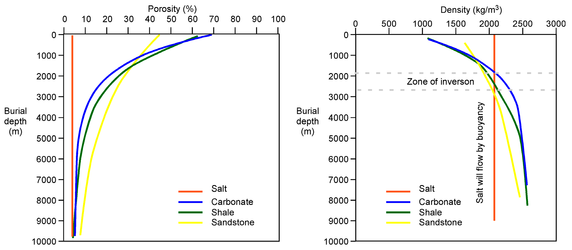
- It behaves as a plastic material under stress. If the applied stress is equal to or larger than a characteristic yield stress, it will flow or creep. Rock creep needs high temperatures, but salt can creep even at room temperature if it contains water [2].
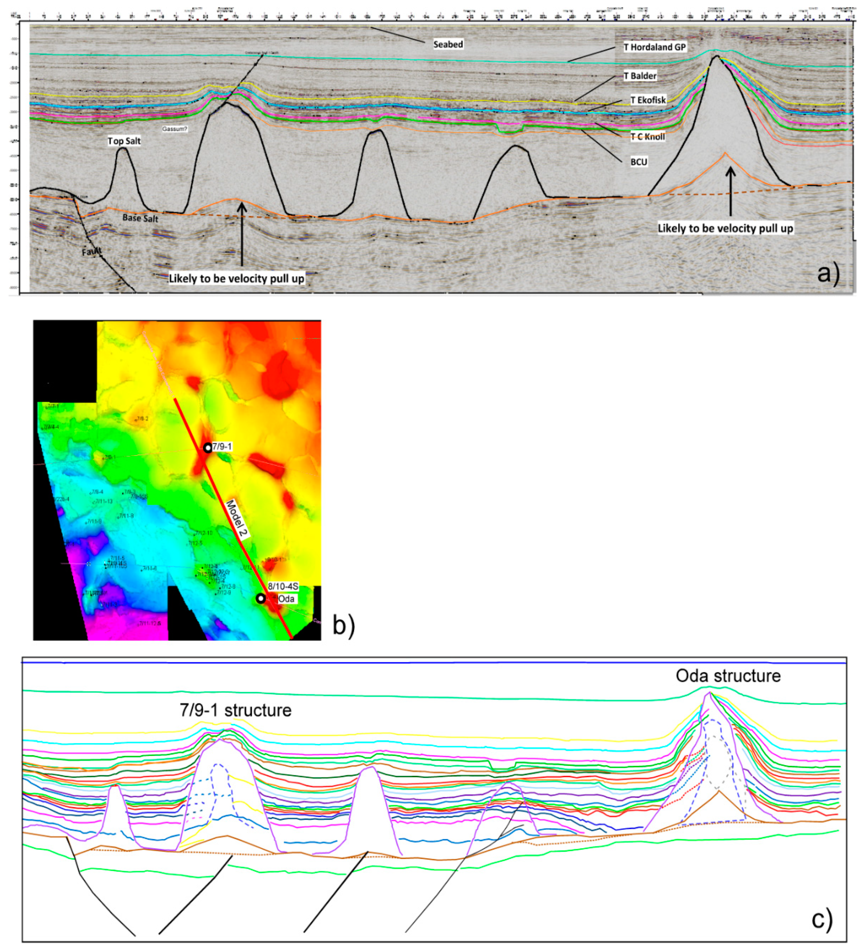
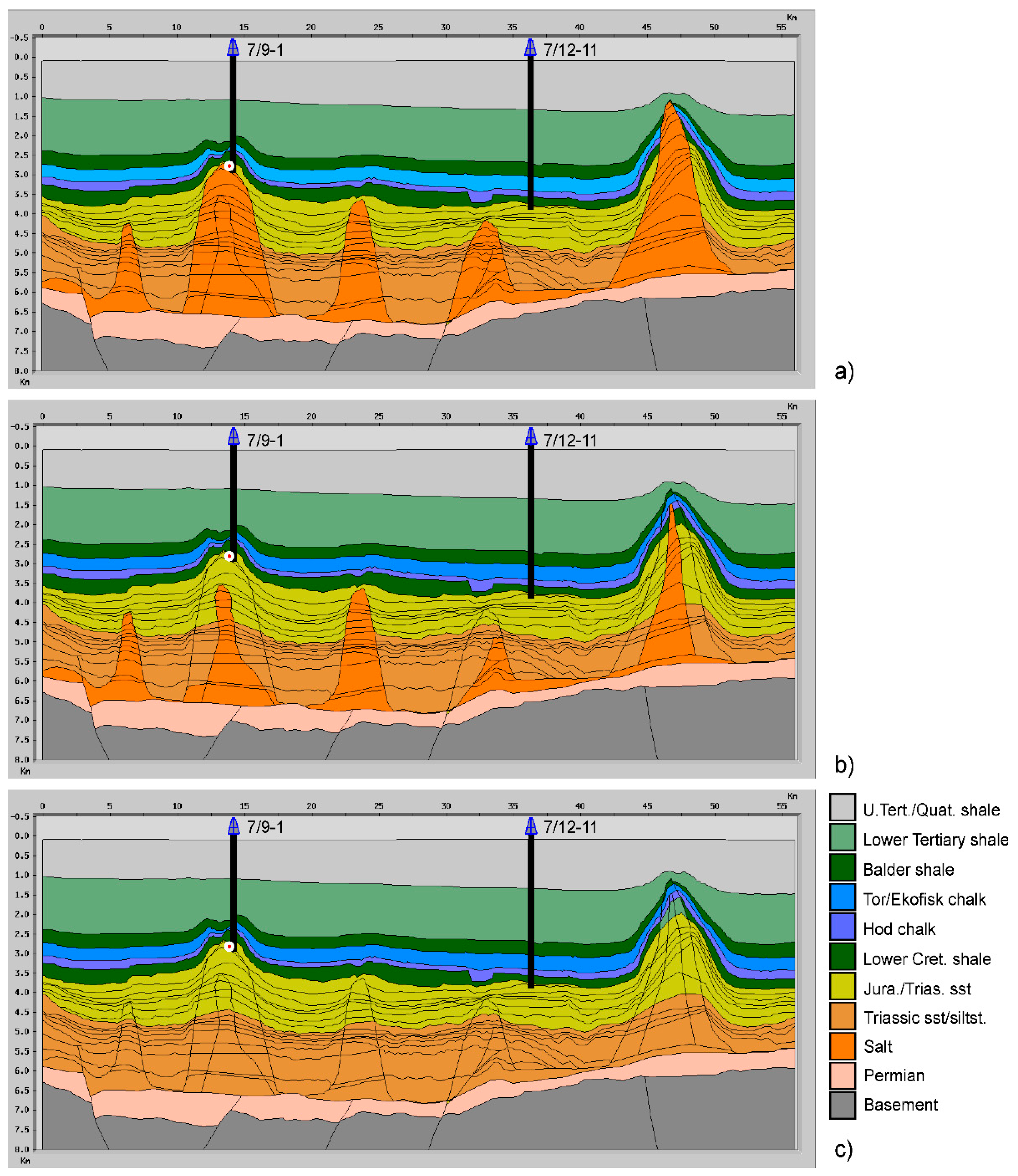
- Salt has high seismic velocity (~4500 m/sec. [6]) leading to unreal “velocity pull-up structures” beneath the salt in seismic time-sections.
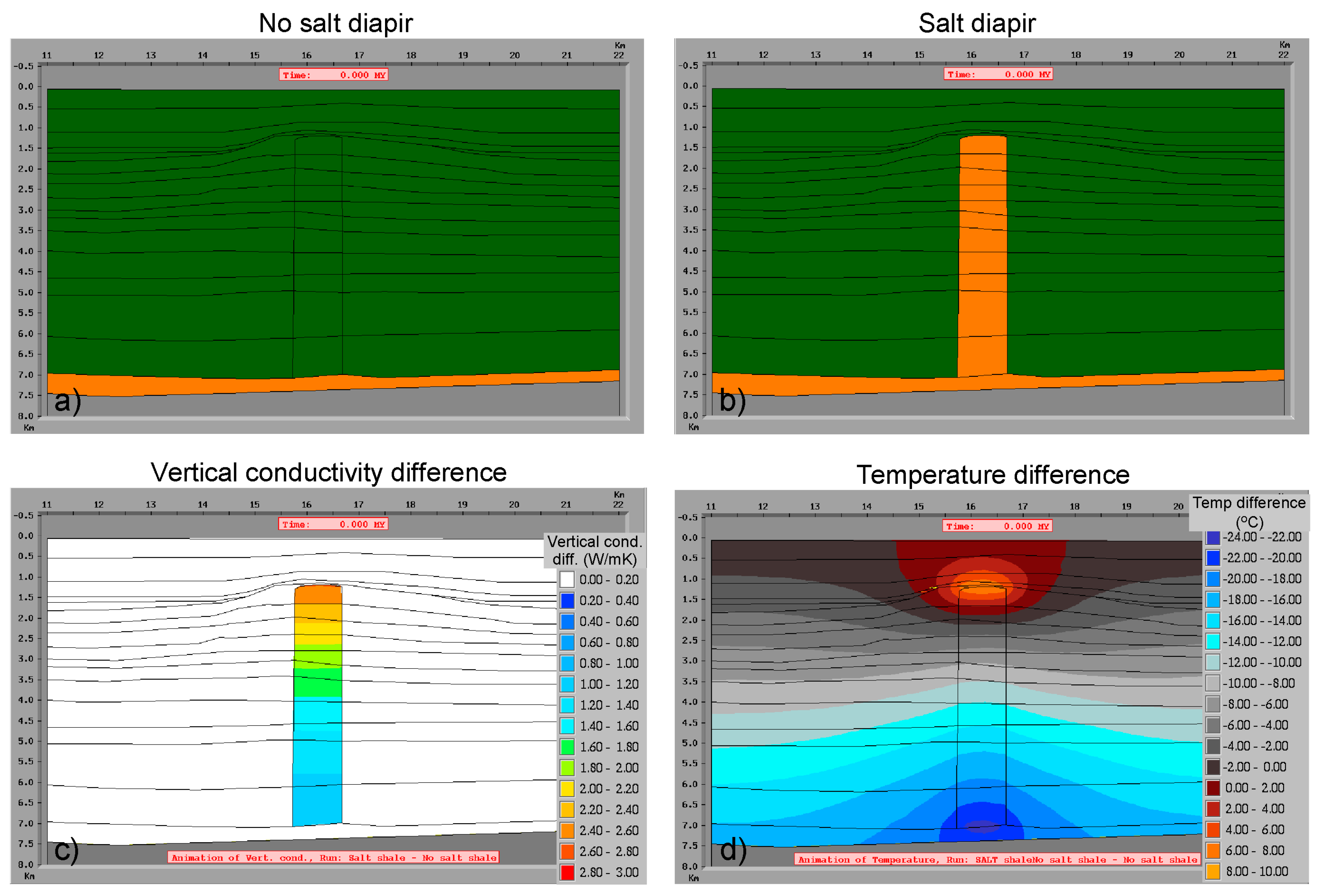
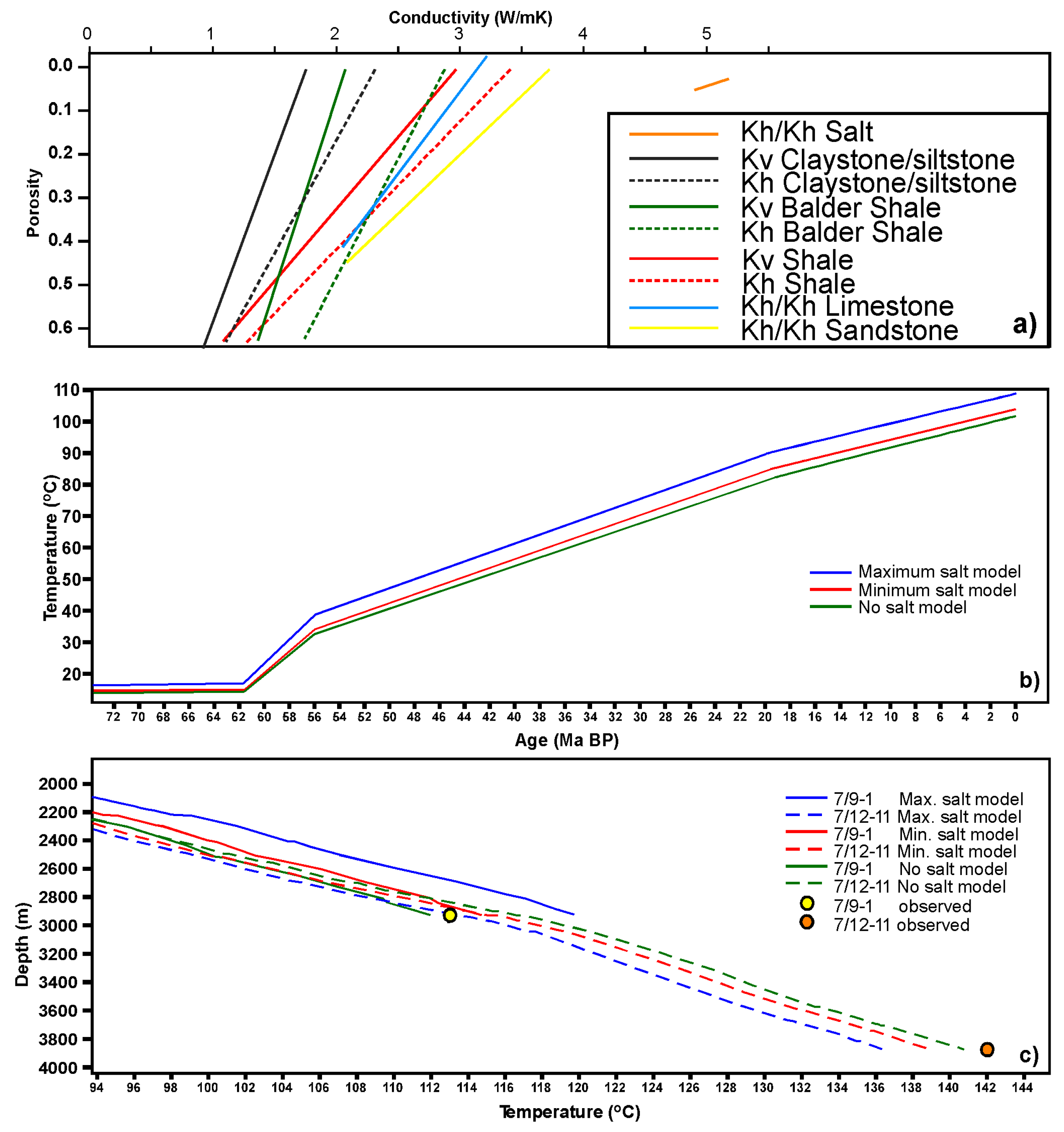
- The thermal conductivity of salt (K) is up to three times greater than the surrounding sediments [7].
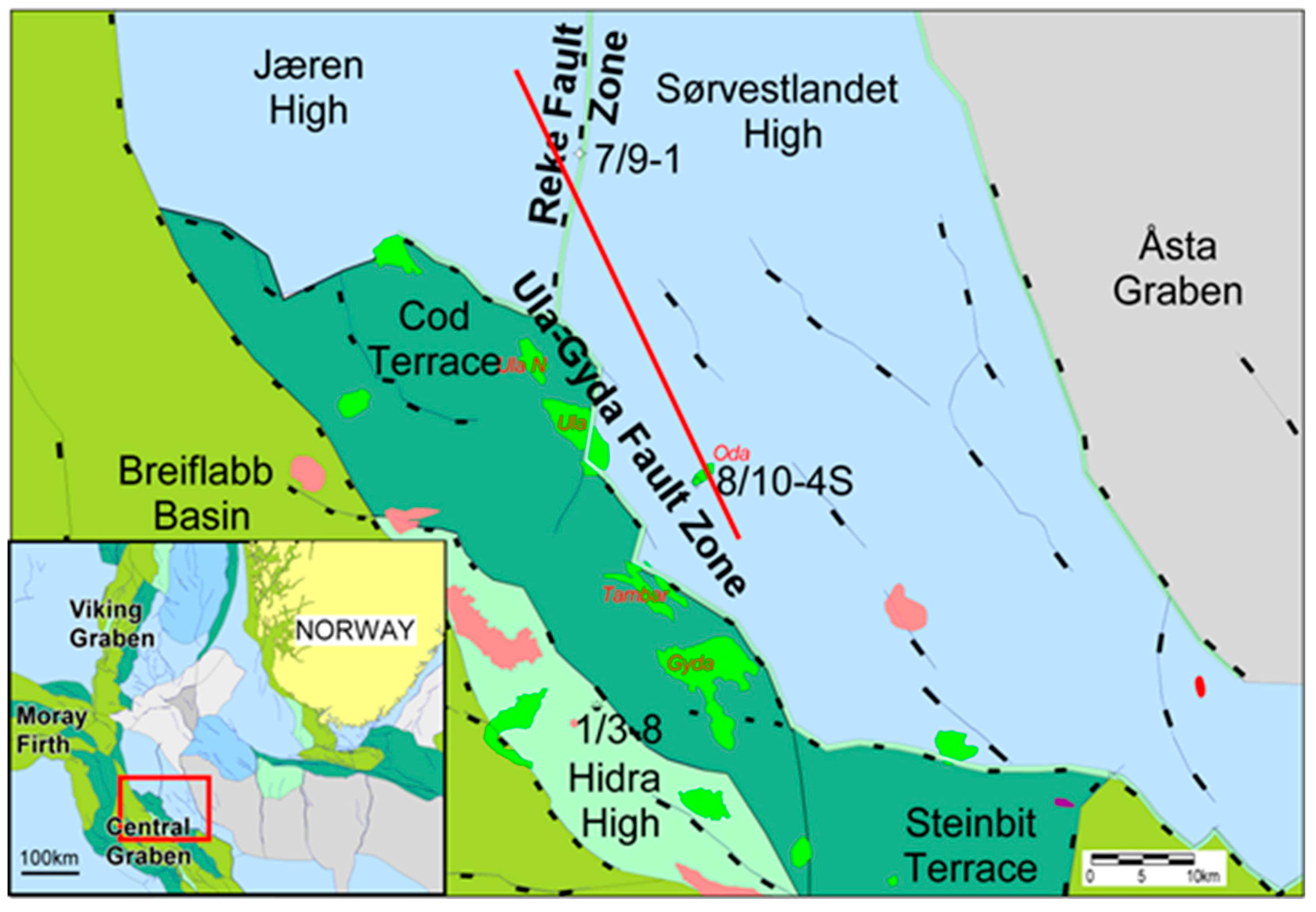
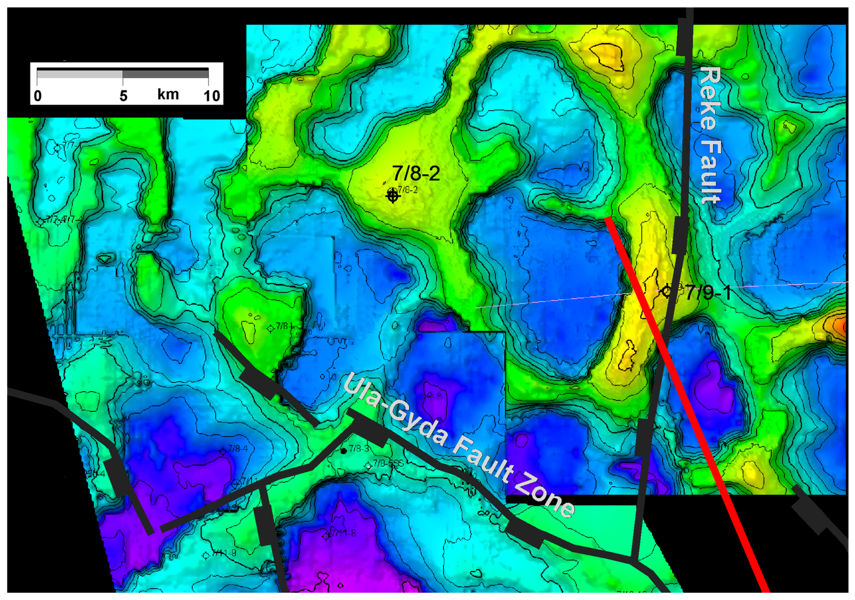
2. Study Area
3. Geology
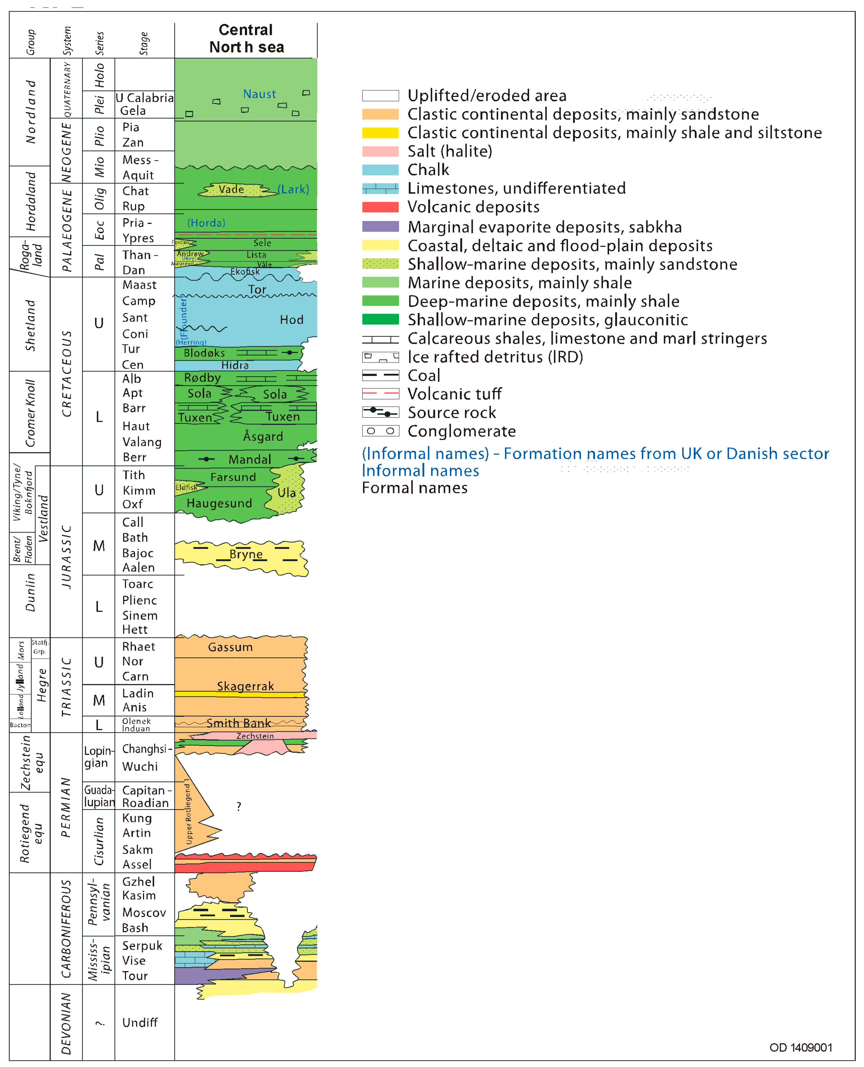
3.1. Stratigraphy
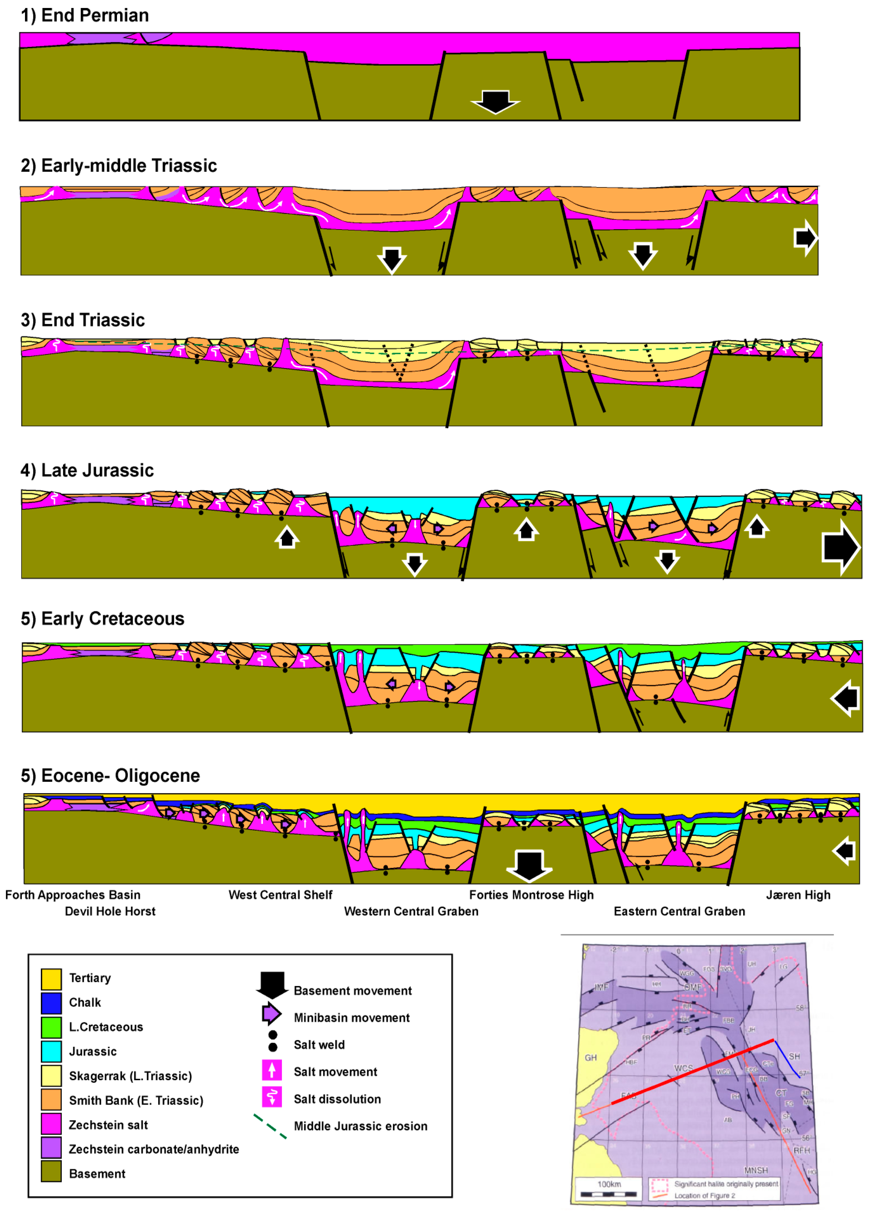
3.2. Triassic Pod Basins
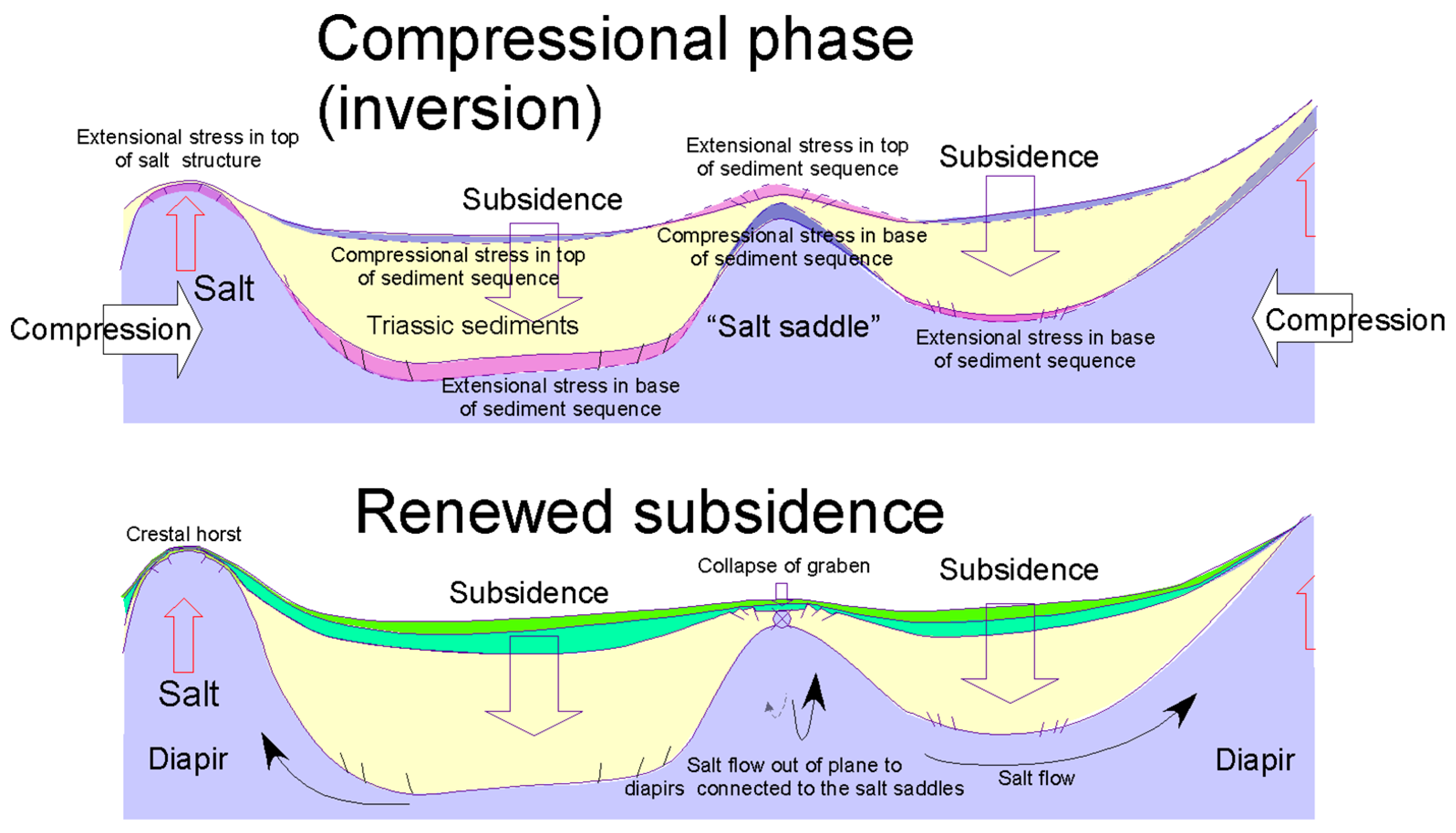
3.3. Cretaceous Collapse Grabens
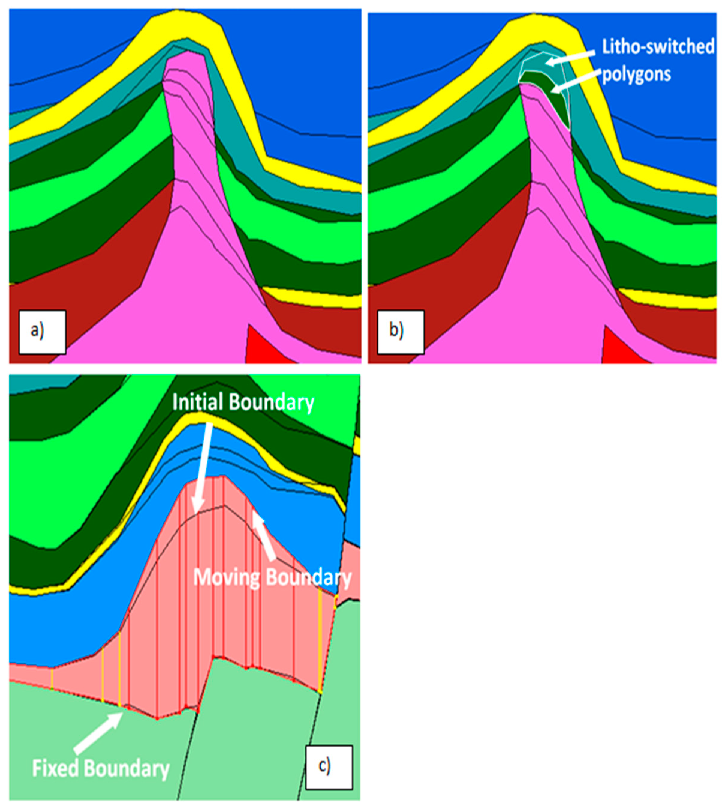
4. Salt Reconstruction Modelling
4.1. Methods
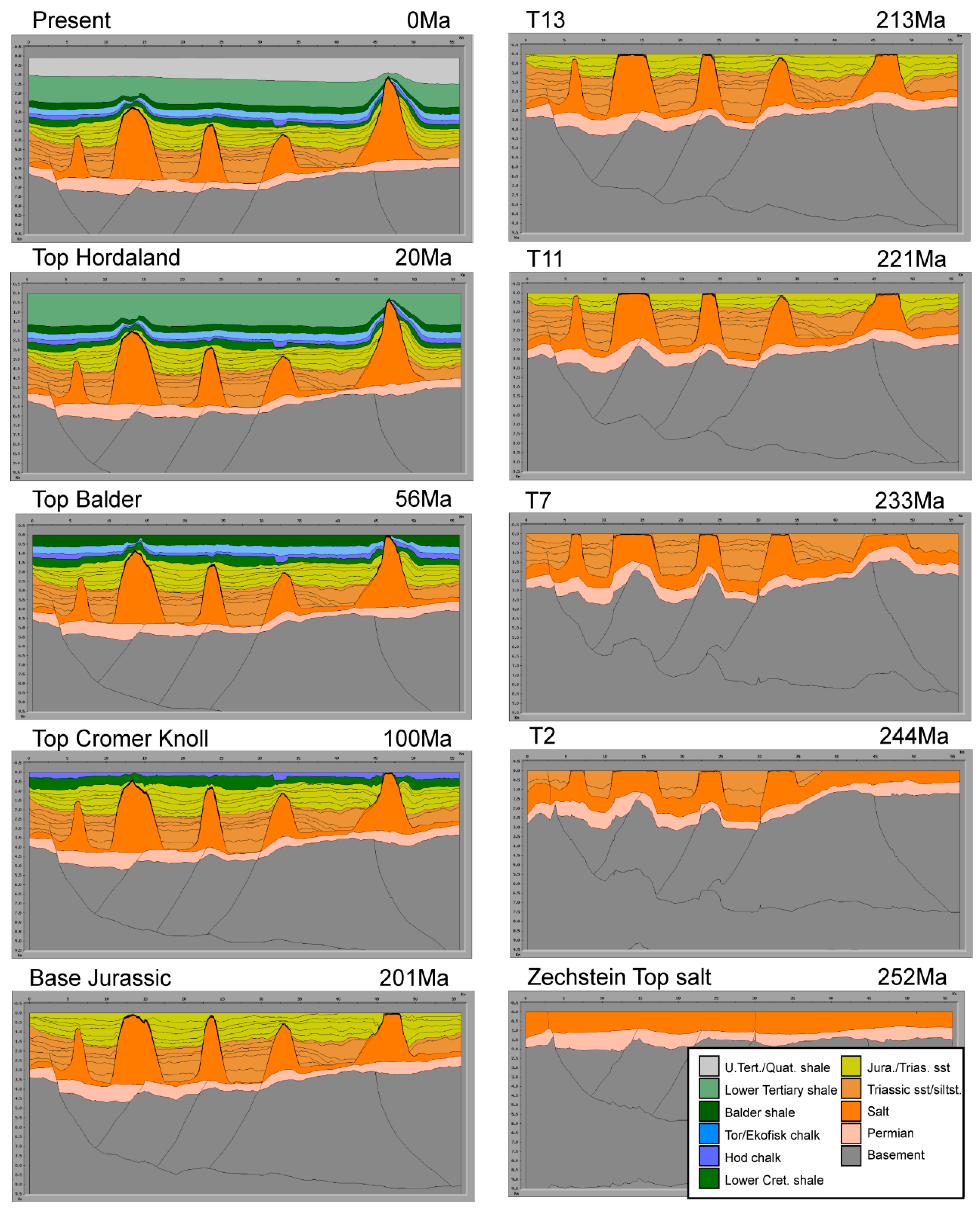
- Reconstruction of the geohistory. The geohistory reconstruction is carried out by a decompaction technique in which the layers are removed one-by-one and corrections are made for the present day compacted thicknesses. The decompaction technique (generally combined with fault-restoration) gives a number of 2D ‘time-slices’ of the basin development.
- Calculation of temperature and maturity history. The calculation is based on the reconstructed geohistory (in i.) using a finite-difference grid. Input for the modeling is paleo heat flow from the mantle, surface temperature history, thermal conductivities, and heat capacities of the sediments. The calculation of vitrinite reflectance is using EASY%RO model.
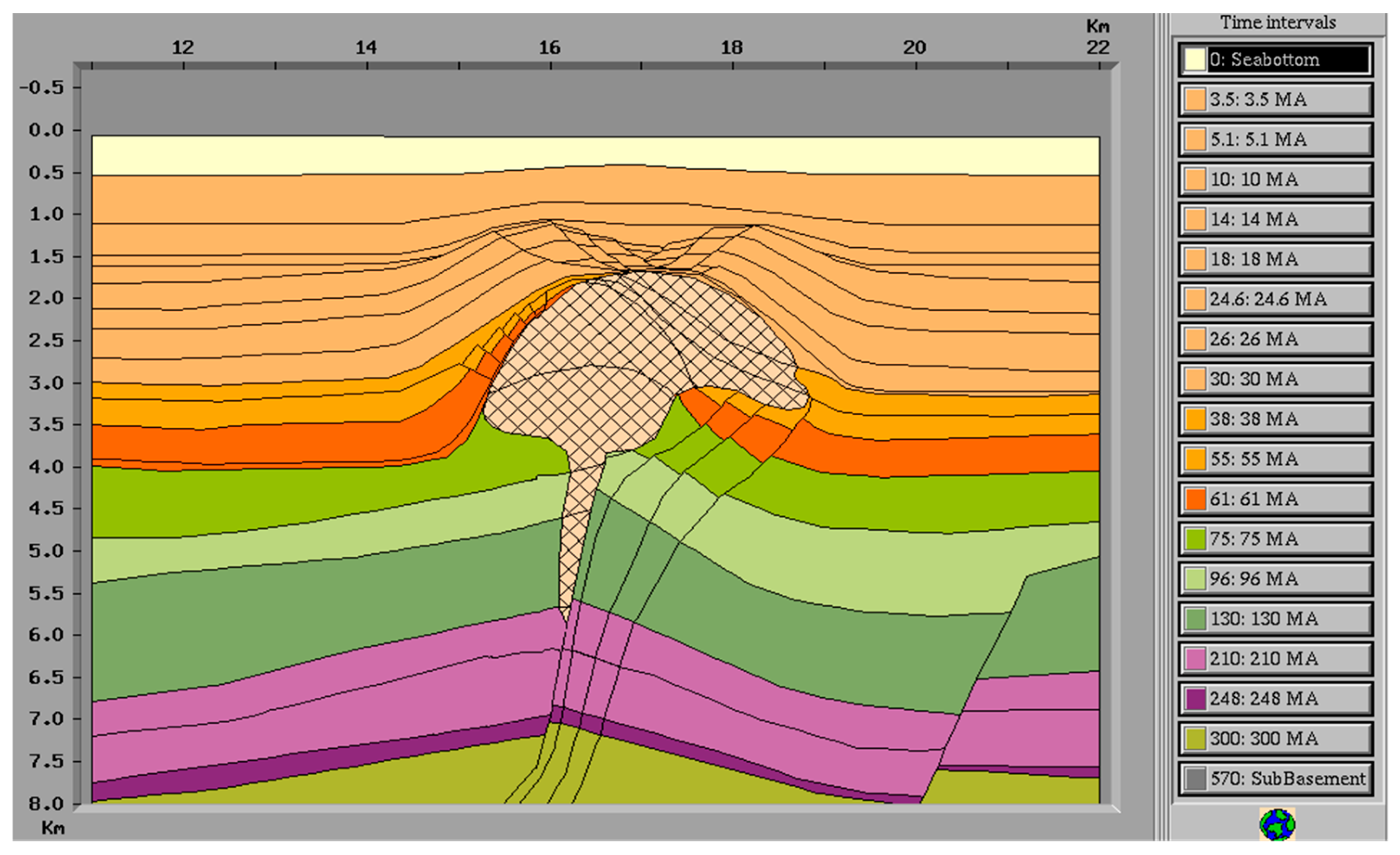
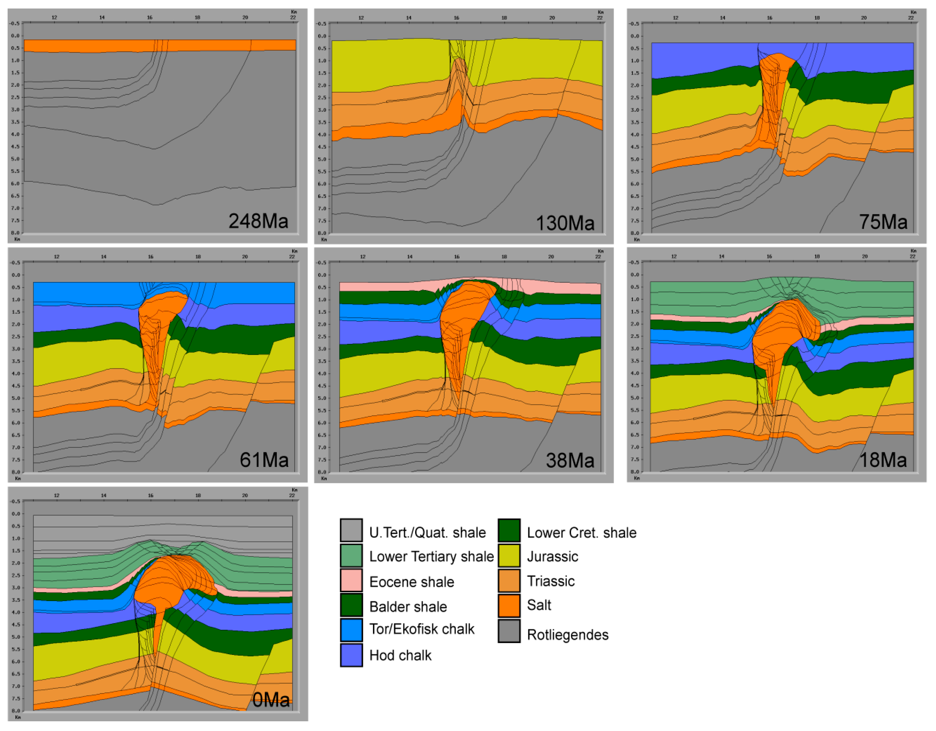
4.2. Geohistory Reconstruction
4.2.1. Model 1
4.2.2. Model 2
5. Modelling of Temperature History and Vitrinite Reflectance
5.1. Temperature Effects of Salt
5.1.1. Synthetic Case
- λ
- is the corrected thermal conductivity in W/m°C
- λref
- is the thermal conductivity calculated at the reference temperature in W/m°C.
- α
- is temperature correction factor in 1/°C, assumed here to be 5.0 10−3 °C
- T
- is the temperature in °C
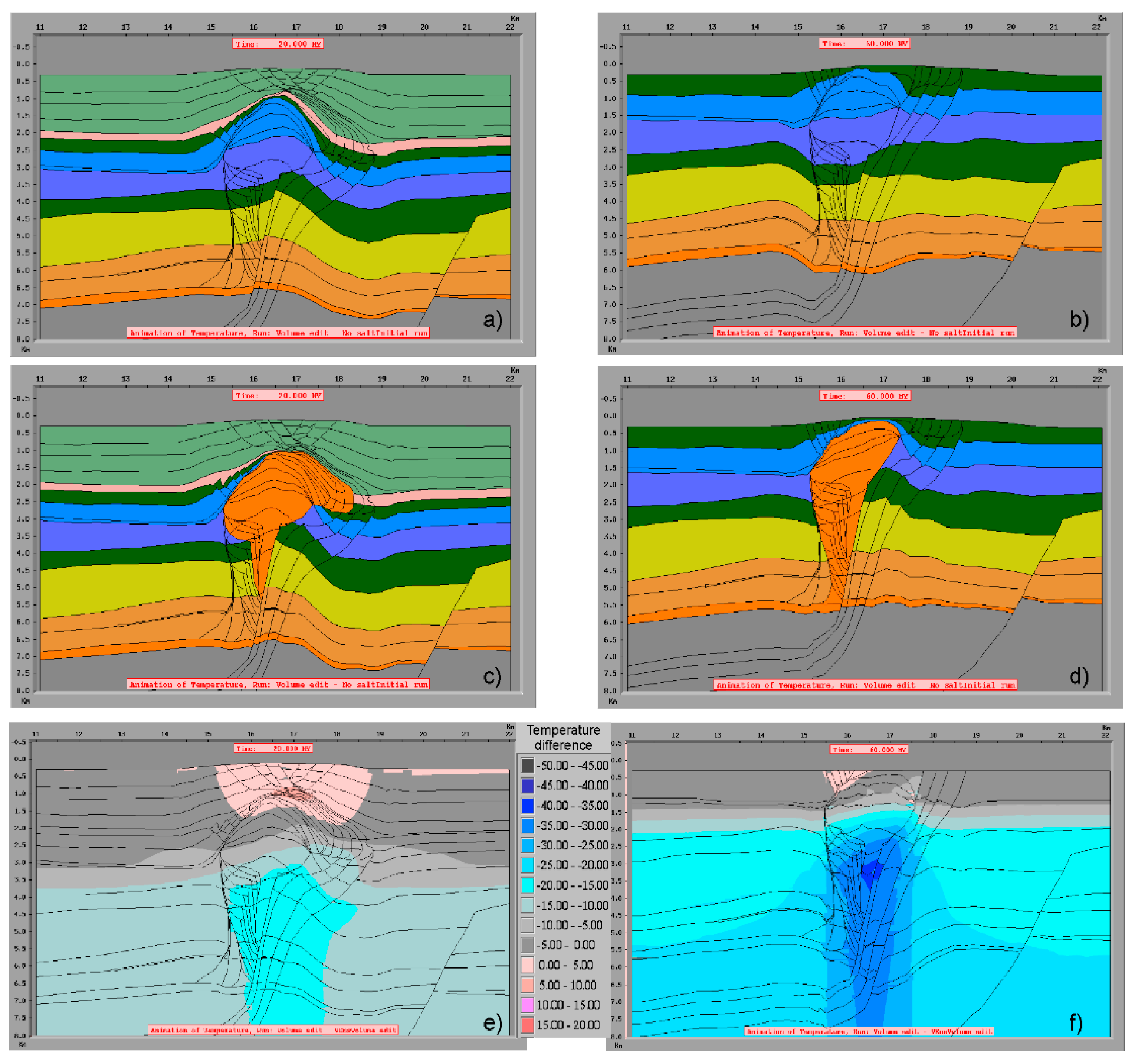
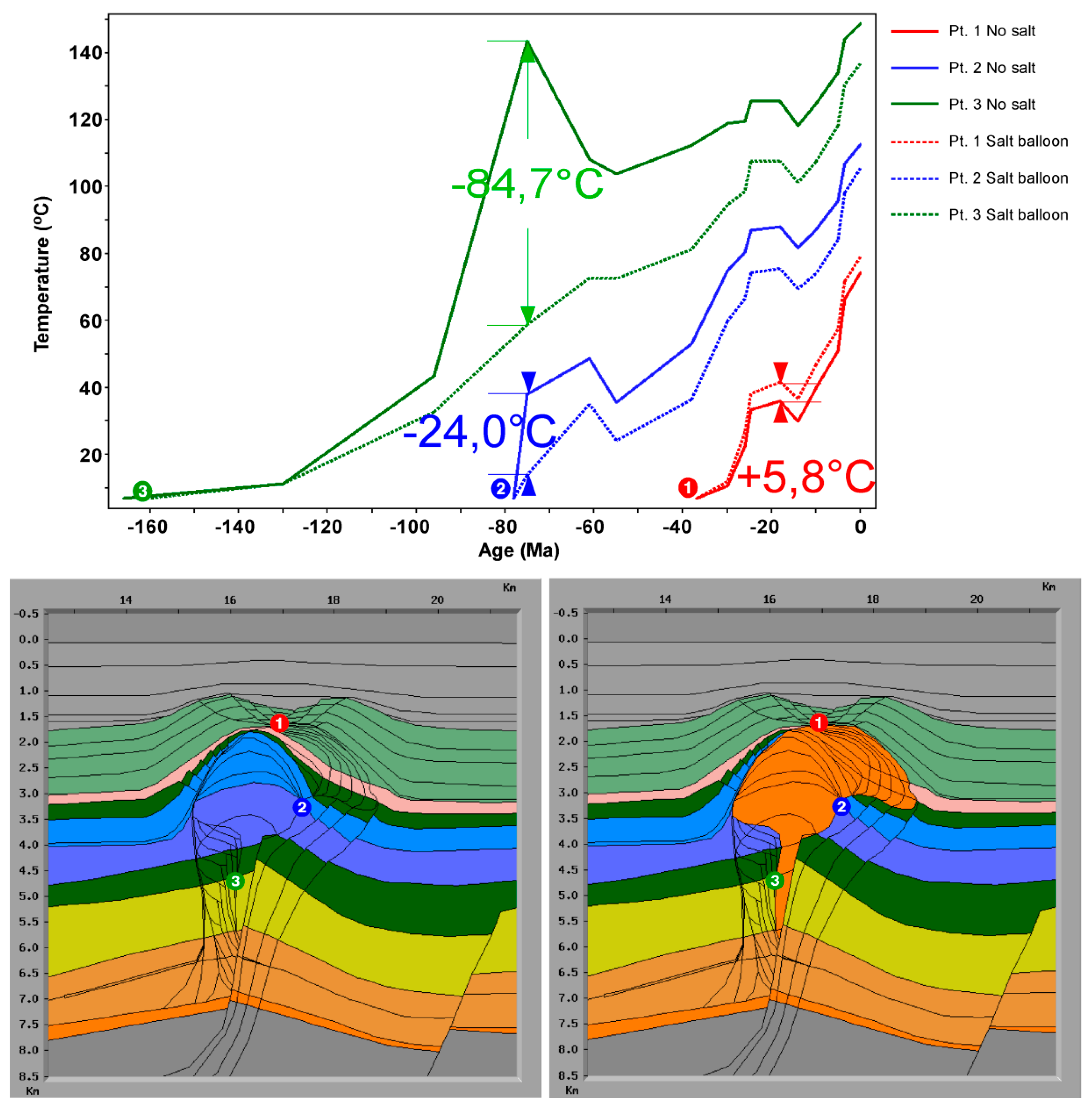
5.1.2. Temperature History of Model 1
5.1.3. Model 2
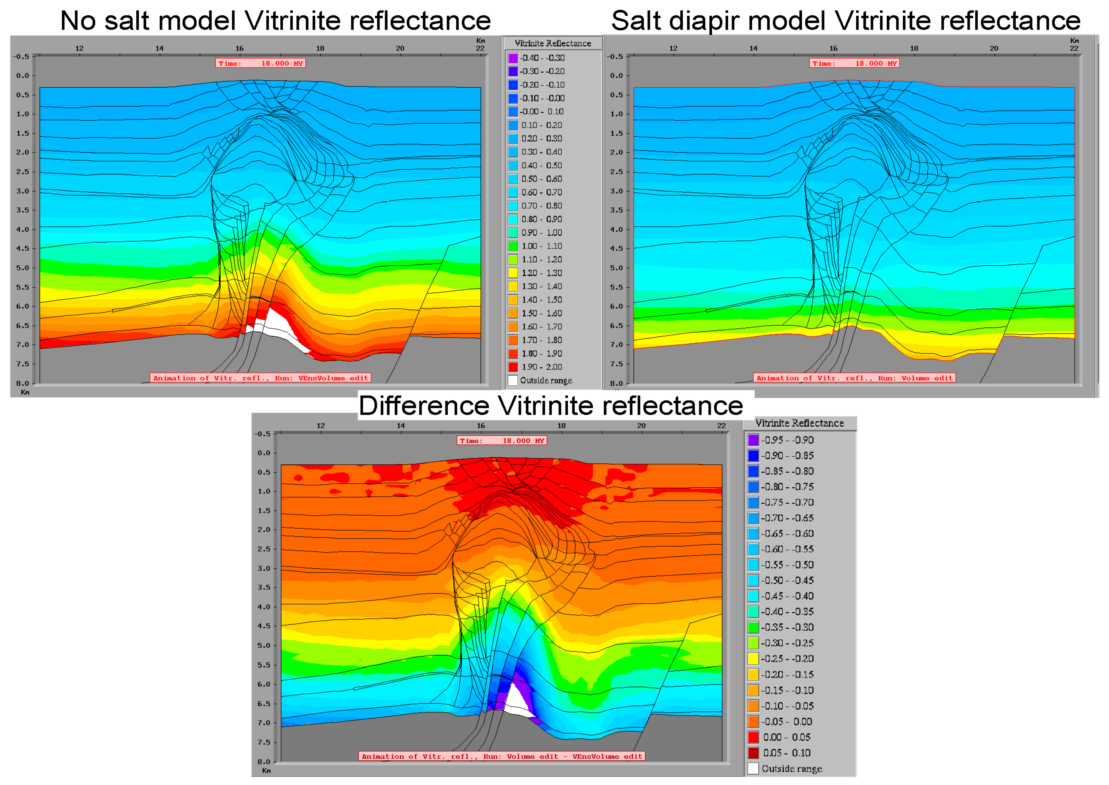
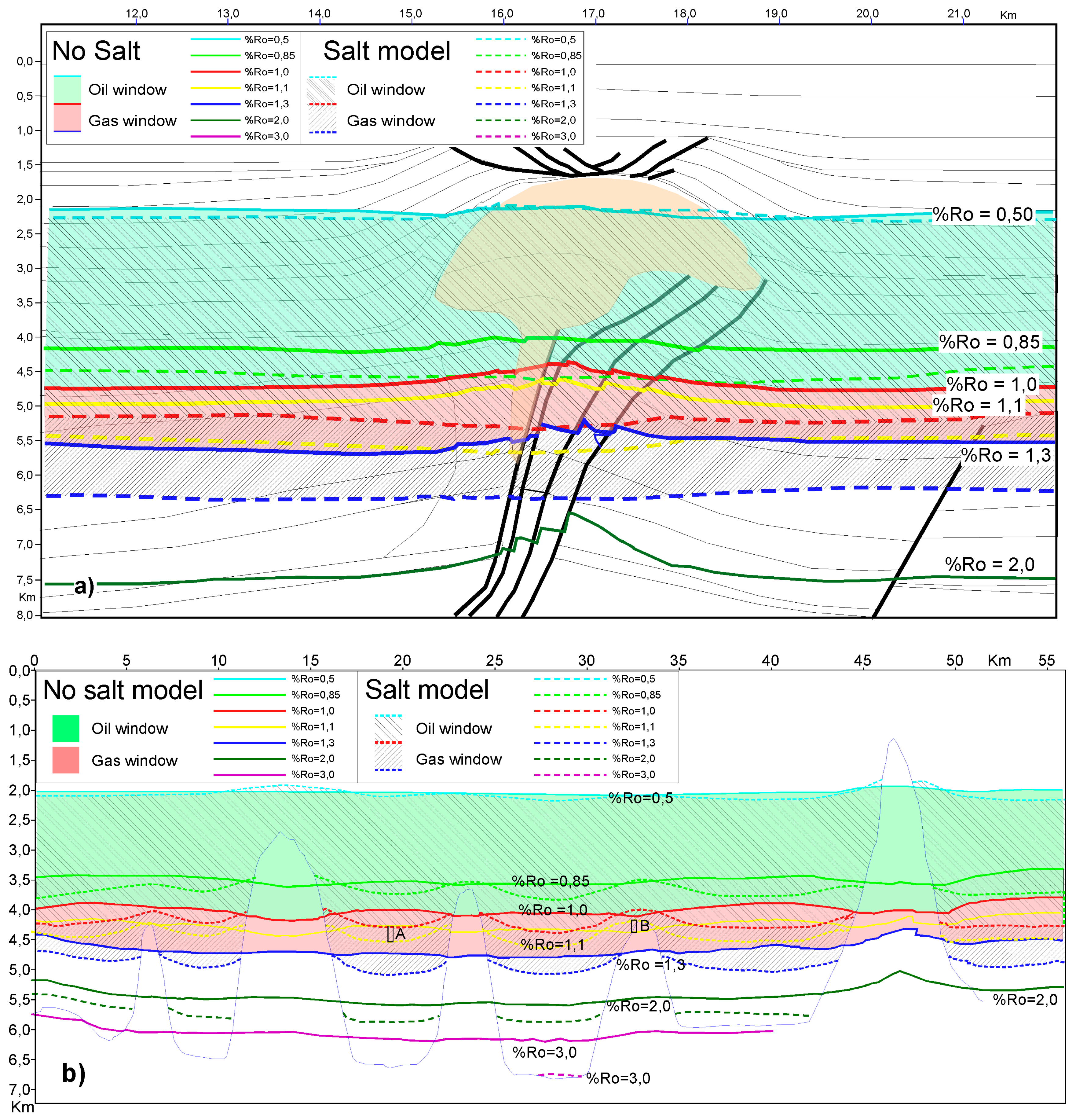
5.2. Vitrinite Reflectance
6. Discussion
7. Conclusions
Author Contributions
Funding
Acknowledgments
Conflicts of Interest
References
- Alsop, G.I.; Archer, S.G.; Hartley, A.J.; Grant, N.T.; Hodgkinson, R. Salt Tectonics, Sediments and Propectivity; Special Publication, Geological Society: London, UK, 2012; 632p. [Google Scholar]
- Jackson, M.P.A.; Hudec, M.R. Salt Tectonics: Principles and Practice; Cambridge University Press: Cambridge, UK, 2017; 510p. [Google Scholar]
- Stewart, S.A.; Clark, J. Impact of salt on the structure of the Central North Sea hydrocarbon fairways. In Petroleum Geology of Northwest Europe: Proceedings of the 5th Conference; Fleet, A.J., Boldy, S.A.R., Eds.; Geological Society: London, UK, 1999; pp. 179–200. [Google Scholar]
- Alsop, G.I.; Weinberger, R.; Marco, S.; Levi, T. Faults and fracture patterns around a strike-slip induced salt wall. J. Struct. Geol. 2018, 106, 103–124. [Google Scholar] [CrossRef]
- Trusheim, F. Mechanism of salt migration in Northern Germany. AAPG Bull. 1960, 44, 1519–1540. [Google Scholar]
- Zong, J.; Coskun, S.; Stewart, R.R.; Dyaur, N.; Myers, M.T. Salt densities and velocities with application to Gulf of Mexico salt domes. In Salt Challenges in Hydrocarbon Exploration SEG Annual Meeting Post-Convention Workshop; Society of Exploration Geophysicists: New Orleans, LA, USA, 2015; Available online: http://www.agl.uh.edu/pdf/jingjing-salt%20densities.pdf (accessed on 24 March 2019).
- Blackwell, D.D.; Steele, J.L. Thermal conductivity of sedimentary rocks: Measurements and significance. In Thermal History of Sedimentary Basins; Naeser, N.D., McColloh, T.H., Eds.; Springer: New York, NY, USA, 1989; pp. 13–37. [Google Scholar]
- Gussow, W.C. Salt diapirism: importance of temperature and energy source of emplacement. In Diapirism and Diapirs; Baraunstein, J., O’Brien, G.D., Eds.; AAPG Mem: Tulsa, OK, USA, 1968; Volume 8, pp. 16–52. [Google Scholar]
- Urai, J.L. Deformation of Wet Salt Rock. Ph.D. Thesis, University of Utrecht, Holland, The Netherlands, 1983. (Referred in Price and Cosgrove, 1990) Unpublished. [Google Scholar]
- Price, N.J.; Cosgrove, J.W. Analysis of Geological Structures; Cambridge University Press: Cambridge, UK, 1990; 502p. [Google Scholar]
- Jackson, M.P.A.; Talbot, C.J. External shapes, strain rates and dynamics of salt structures. Geol. Soc. Am. Bull. 1986, 97, 305–323. [Google Scholar] [CrossRef]
- Hudec, M.R.; Jackson, M.P.A. Terra infirma: Understanding salt tectonics. Earth-Sci. Rev. 2007, 82, 1–28. [Google Scholar] [CrossRef]
- Brun, J.-P.; Fort, X. Salt tectonics at passive margins: Geology versus models. Mar. Pet. Geol. 2011, 28, 1123–1145. [Google Scholar] [CrossRef]
- Mello, U.T.; Karner, G.D.; Anderson, R.N. Role of salt in restraining the maturation of subsalt source rocks. Mar. Pet. Geol. 1995, 12, 697–716. [Google Scholar] [CrossRef]
- Baniak, G.M.; Gingras, M.K.; Burns, B.A.; Pemberton, S.G. An example of a highly bioturbated, storm-influenced shoreface deposit: Uper Jurassic Ula Formation, Norwegian North Sea. Sedimentology 2014, 61, 1261–1285. [Google Scholar] [CrossRef]
- Hodgson, N.A.; Farnsworth, J.; Fraser, A.J. Salt-related tectonics, sedimentation and hydrocarbon plays in the Central Graben, North Sea, UKCS. Geol. Soc. Lond. Spec. Publ. 1992, 67, 31–63. [Google Scholar] [CrossRef]
- Karlo, J.F.; van Buchem, F.S.P.; Moen, J.; Milroy, K. Triassic-age salt tectonics of the Central North Sea. Interpretation 2014, 2, SM19–SM28. [Google Scholar] [CrossRef] [Green Version]
- Mannie, A.S.; Jackson, C.A.L.; Hampson, G.J. Shallow-marine reservoir development in extensional diapir-collapse minibasins: An integrated subsurface case study from the Upper Jurassic of the Cod terrace, Norwegian North Sea. AAPG Bull. 2014, 98, 2019–2055. [Google Scholar] [CrossRef]
- Mannie, A.S.; Jackson, C.A.L.; Hampson, G.J.; Fraser, A.J. Tectonic controls on the spatial distribution and stratigraphic architecture of net-transgressive shallow- marine synrift succession in a salt-influenced rift basin: Middle to Upper Jurassic, Norwegian Central North Sea. J. Geol. Soc. 2016, 173, 901–915. [Google Scholar] [CrossRef]
- Høiland, O.; Kristensen, J.; Monsen, T. Mesozoic evolution of the Jæren High area, Norwegian Central North Sea. In Petroleum Geology of Northwest Europe: Proceedings of the 4th Conference; Parker, J.R., Ed.; Geological Society: London, UK, 1993; pp. 1189–1195. [Google Scholar]
- Pegrum, R.M. Structural development of the south-western margin of the Russian-Fennoscandian Platform. In Petroleum Geology of the Northern European Margin; Spencer, A.M., Ed.; Graham & Trotman: London, UK, 1984; pp. 173–189. [Google Scholar]
- Fjeldskaar, W.; Ter Voorde, M.; Johansen, H.; Christiansson, H.P.; Faleide, J.I.; Cloetingh, S.A.P.L. Numerical simulation of rifting in the northern Viking Graben: the mutual effect of modelling parameters. Tectonophysics 2004, 382, 189–212. [Google Scholar] [CrossRef]
- Fjeldskaar, W.; Andersen, Å.; Johansen, H.; Lander, R.; Blomvik, V.; Skurve, O.; Michelsen, J.K.; Grunnaleite, I.; Mykkeltveit, J. Bridging the gap between basin modelling and structural geology. Reg. Geol. Metallog. 2017, 72, 65–77. [Google Scholar]
- Sclater, J.G.; Christie, P. Continental stretching: an explanation of the post-mid-Cretaceous subsidence of the Central North Sea basin. J. Geophys. Res. 1980, 85, 3711–3739. [Google Scholar] [CrossRef]
- Fernandez, N.; Jackson, C.A.L.; Hudec, M.; Dooley, T.P. The Competition for Salt and Kinematic Interactions between Minibasins during Density-Driven Subsidence Observations from Numerical Models. 2019. Available online: https://www.researchgate.net/publication/331904078_ (accessed on 4 August 2019).
- Burrus, J.; Audebert, F. Thermal and compaction processes in a young rifted basin containing evaporties: Gulf of Lions, France. AAPG Bull. 1990, 74, 1420–1440. [Google Scholar]
- Crelling, J.C.; Dutcher, R.R. Principles and Applications of Coal Petrology: SEPM Short; Course. Society of Economic Paleontologists Mineralogists: Tulsa, OK, USA, 1980; Volume 8, 127p. [Google Scholar]
- Sweeney, J.J.; Burnham, A.K. Evolution of a simple model of vitrinite reflectance based on chemical kinetics. AAPG Bull. 1990, 74, 1559–1570. [Google Scholar]
- Fjeldskaar, W.; Prestholm, E.; Guargena, C.; Gravdal, N. Isostatic and tectonic development of the Egersund Basin. In Basin Modelling: Advances and Applications; Doré, T., Augustson, J.H., Hermanrud, C., Stewart, D.J., Sylta, Ø., Eds.; Elsevier: Amsterdam, The Netherlands, 1993; pp. 549–562. [Google Scholar]
- Davison, I.; Alsop, G.I.; Evans, N.G.; Safarics, M. Overburden deformation patterns and mechanisms of salt diapir penetration in the Central Graben, North Sea. Mar. Pet. Geol. 2000, 17, 601–618. [Google Scholar] [CrossRef]


| Lithology | Surface Porosity Fo | Exponential Porosity Constant c | Thermal Conductivity (W/mK) | Specific Heat Capacity (J/kg K) |
|---|---|---|---|---|
| Claystone and siltstone | 0.63 | 0.51 | 1.7 (6% porosity) 1.0 (60% porosity) | 940 |
| Shale | 0.63 | 0.51 | 2.8 (6% porosity) 1.2 (60% porosity) | 1190 |
| Chalk | 0.70 | 0.71 | 2.04 (13% porosity) 1.23 (38% porosity) | 1090 |
| Sandstone Jurassic | 0.37 | 0.58 | 2.04 (13% porosity) 1.23 (36% porosity) | 1090 |
| Sandstone Triassic | 0.49 | 0.27 | 3.4 (6% porosity) 2.5 (40% porosity) | 1080 |
| Salt | 0.04 | 0.05 | 5.1 (3% porosity) 5.0 (4% porosity) | 1060 |
| Basement | 0.04 | 0.05 | 3.1 (3% porosity) 3.1 (4% porosity) | 1100 |
© 2019 by the authors. Licensee MDPI, Basel, Switzerland. This article is an open access article distributed under the terms and conditions of the Creative Commons Attribution (CC BY) license (http://creativecommons.org/licenses/by/4.0/).
Share and Cite
Grunnaleite, I.; Mosbron, A. On the Significance of Salt Modelling—Example from Modelling of Salt Tectonics, Temperature and Maturity Around Salt Structures in Southern North Sea. Geosciences 2019, 9, 363. https://doi.org/10.3390/geosciences9090363
Grunnaleite I, Mosbron A. On the Significance of Salt Modelling—Example from Modelling of Salt Tectonics, Temperature and Maturity Around Salt Structures in Southern North Sea. Geosciences. 2019; 9(9):363. https://doi.org/10.3390/geosciences9090363
Chicago/Turabian StyleGrunnaleite, Ivar, and Arve Mosbron. 2019. "On the Significance of Salt Modelling—Example from Modelling of Salt Tectonics, Temperature and Maturity Around Salt Structures in Southern North Sea" Geosciences 9, no. 9: 363. https://doi.org/10.3390/geosciences9090363
APA StyleGrunnaleite, I., & Mosbron, A. (2019). On the Significance of Salt Modelling—Example from Modelling of Salt Tectonics, Temperature and Maturity Around Salt Structures in Southern North Sea. Geosciences, 9(9), 363. https://doi.org/10.3390/geosciences9090363