Abstract
A model for the extraction and quantitative characterization of submarine landforms from high-resolution digital bathymetry is presented. The procedure is fully automated and comprises two parts. The first part consists of an analytical model which extracts quantitative information from a Digital Elevation Model in the form of objects with similar parametric characteristics (terrain objects). The second part is a rule-based model where the terrain objects are reclassified into distinct landforms with well-defined three dimensional characteristics. For the focus of this work, the quantitative characterization of isolated dunes (height greater than 2 m) is used to exemplify the process. The primary metrics used to extract terrain objects are the flatness threshold and the search radius, which are then used by the analytical model to identify the feature type. Once identified as dunes, a sequence of spatial analysis routines is applied to identify and compute metrics for each dune including length, height, width, ray of curvature, slope analysis for each stoss and lee side, and dune symmetry. Dividing the model into two parts, one scale-dependent and another centered around the shape of the landform, makes the model applicable to other submarine landforms like ripples, mega-ripples, and coral reefs, which also have well-defined three-dimensional characteristics.
1. Introduction
There is evidence that the shape of the earth, at many scales, directly affects the spatial distribution of life. This connection between landscapes and organisms is bidirectional, where “the land is shaped by life, [and] life is shaped by the landscapes it inhabits” [1,2]. This two-way interaction between species and environment, including geomorphology, is an important object of study in ecology and is at the basis of niche theory as well as the foundation of the concept of habitat [3].
Mapping of seafloor habitat is an essential element to understanding the ecology of the benthic zone. By acquiring knowledge of seafloor characteristics and benthic community structure, habitat mapping is a useful tool for many purposes ranging from the study of marine biodiversity, design of marine protected areas, and planning marine fishing reserves [4]. In particular, habitat mapping is crucial for the development of marine resource management plans maintaining a sustainable fishing industry and gauging the performance of existing management plans.
The linkage between abiotic and biotic components of a specific set of species in a well-defined environmental setting is what is used in ecology to identify a particular habitat (or biotope). Species distribution modeling is a complex and multidisciplinary scientific art that studies still poorly understood interactions. It involves multidimensional environmental analyses, where models built on top of “explanatory variables” (predictors) are tested against a few detailed and accurate observations (ground truth). Those observations can be species presence/absence, species abundance, species assemblage, etc.
Much work has been done to relate geomorphology and biological composition. A relationship between physical properties of the seafloor and the occurrence of certain species assemblages has been demonstrated in some studies (e.g., [5,6]), but such linkage is still poorly understood, and it is the object of ongoing research in marine ecology. Many studies (e.g., [4], Table 5.2) report seafloor morphology and sediment type as the most important variables explaining the spatial distribution of benthic species assemblages. Such habitat surrogates can be extracted from bathymetry and acoustic backscatter mosaics derived by Multibeam Echosounder (MBES) data [7,8]. Thus, depending on the scale of the analysis, MBES is one of the most valuable tools to study seafloor habitat.
This study focuses on the application of quantitative models of Digital Bathymetric Models (DBM) to characterize morphology by landform extraction. The quantitative approaches described are the theoretical foundation of Digital Terrain Analysis (DTA).
The quantitative description of a form, morphometry, applied to the Earth’s surface is what is known, in physical geography, as geomorphometry [9]. Geomorphometry can be divided into general geomorphometry, which analyzes the land surface as a ontinuous surface described by local attributes, and specific geomorphometry which relates to a specific surface’s features and deals with their quantitative description. Specific geomorphometry can then be defined as the process of subdivision of the terrain into landforms based on a segmentation process and then the characterization of each segment based on their relationship to one another [10]. DTA allows the partitioning of the landscape into objects with a distinct parametric representation resulting from a standard combination of processes, materials, and conditions. Such objects (or relief features) are often called landforms. Each landform exhibits a predictable range of visual and physical characteristics [11] and the analysis of such characteristics is the object of the study of specific geomorphometry.
Unfortunately, approaches for classifying and segmenting land surfaces into useful units are often tuned to model local processes with explicit assumptions and limitations that only apply to the local conditions [12]. Variables such as grid resolution and size of the neighborhood operators have a large influence on the terrain derivatives used by landform recognition models [13] affecting their ability to detect all the terrain features that characterize a landscape. Moreover, to correlate landforms with geological processes, a specific set of rules is usually implemented, which will work only for that particular process. Hence, a unique, generic terrain-classification framework that will work for any geological process is difficult, if not impossible, to achieve.
The objective of this paper is to develop an approach to analyzing digital bathymetric models in order to identify and quantitatively describe specific bedforms with the final goal of achieving a better understanding of the geological and physical settings of the area that can be used for habitat characterization and other studies.
Presented is an approach for detection, extraction and quantitative characterization of a particular seascape. The approach first makes use of specific morphometry techniques to extract terrain features including ridges, slopes, summits, spurs, etc. from high-resolution digital bathymetry and identify the feature. Then, it uses these terrain features to extract and quantitatively characterize specific submarine bedforms. We used large, isolated sand dunes as the example bedform in this paper.
This study is part of ongoing research which aims to characterize the benthic habitats of the Great South Channel (GSC) through the use of the Coastal and Marine Ecological Classification Standard (CMECS). The Great South Channel is characterized by the widespread presence of large sand dunes, varying in scale and type. One of the requirements of the CMECS is the characterization of major geomorphic and structural characteristics of the seafloor at various levels of detail, which are described in the CMECS geoform component [14], and which motivated the development of the present method. The seafloor characterization tool presented in this paper will be used to identify and quantitatively characterize these particular bedforms and their associated biotopes.
2. Methods
2.1. Area of Study
The analysis in this study focuses on an area located on the western boundary of Georges Bank, 50 nautical miles east of Nantucket Island in the proximity of the west side of the Great South Channel at the southern border of the Gulf of Maine (Figure 1). Georges Bank is a relatively shallow (less than 200 m) bank composed mostly of glacial debris transported from the continent in the late Pleistocene [15] and constantly reworked by strong M2 tidal currents [16]. Due to the interaction of a complex current system and its bathymetry, Georges Bank is considered one of the most productive shelf ecosystems in the world [16,17,18,19,20,21] with a primary production that reaches 400–500 gC yr [22].
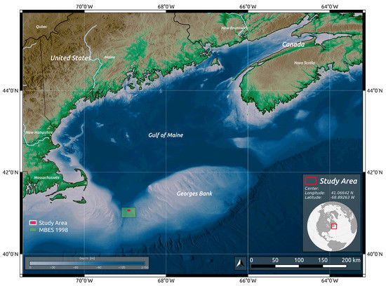
Figure 1.
Location of the area of study (red circle), USGS MBES survey (1998) [23] (green area). The shaded relief used as background is derived from the 3 arc second digital elevation model of the Gulf of Maine, source: United States Geological Survey (USGS)—Coastal and Marine program, Woods Hole (MA).
The area is characterized by major topographic features formed by glacial and postglacial processes [23]. The east side of the DBM presents a cluster of giant dunes in a sediment-rich area, whereas the west side is characterized by large and isolated dunes (Figure 2) in a sediment-starved area, with coarser sediments and presence of boulders probably resulting from ice-rafted debris. The whole area is subject to a strong tidal regime with a fast and strong southward outflow and a weaker but longer northward inflow. In addition, the area is occasionally affected by strong storm currents. All these processes maintain the seabed in a status of dynamic equilibrium with active sediment transport.
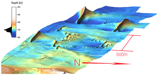
Figure 2.
Details of the morphology of the study area (elevation exaggeration ).
2.1.1. Survey Description
The study area covered approximately , with an average depth of 90 m, gently deepening towards the west with an absolute difference in depth of 30 m. Due to the strong tidal regime, all fine sediment in the area is washed away by currents, leaving the seabed covered by a surficial layer of coarse-grained sand and gravel. In such an environment, well-distinguished bedforms such as ripples, mega-ripples, and sand dunes are common (Figure 2).
The data included the acquisition of high-resolution multibeam bathymetry co-registered with a continuous ribbon of still stereographic photos of the seafloor along with the acquisition of a number of water column parameters and physical and biological samples.
2.1.2. Survey Methods
High-resolution multibeam sonar bathymetry and acoustic backscatter data were collected with a Reson Seabat 7125 SVP2 ( Teledyne Reson, Slangerup, Denmark). The multibeam echosounder was installed on one of the three drop keel frames of the University of Delaware research vessel, R/V Hugh R. Sharp. The sonar was operated at a frequency of 400 kHz and a swath width of 150 degrees. The system was integrated with an Applanix Pos-MV 320 V5 GPS Positioning System which provided accurate altitude, heading, heave, position and velocity of the vessel. This information was used to correct the data for motion artifacts. The survey consisted of eleven parallel track lines running in a east-west direction with a spacing of 20 m. Continuous high-resolution still photographic imagery of the seafloor was collected in the survey area with Prosilica Giga Ethernet stereo cameras mounted on the HabCam system [24]. The co-registration of images and acoustic data was possible by deploying an Ultra Short Baseline (USBL) underwater positioning system, which provided accurate tracking of the HabCam. The USBL Transducer was installed on the second drop down keel frame of the R/V Hugh R. Sharp, with a known offset from the POS/MV. The Beacon/Pinger was mounted on the top frame of the HabCam, in the proximity of the mounting hook of the fiber optic cable. The system was calibrated at the beginning of the cruise by deploying a beacon on the seafloor at a depth of 60 m and performing a static calibration using the four cardinal point scheme, which was possible thanks to the dynamic positioning (DP) capabilities of the R/V Hugh R. Sharp. The four cardinal point scheme calibration method was indicated by USBL manufacturer and is considered the most appropriate calibration method [25]. All the mapping and sampling equipment on the R/V Sharp were synchronized with a time server for accurate time-stamping of the data logs. The survey data also included sediment samples from three box-core stations and biological observations including species, number of individuals, as well as sex and size from a long dredge tow in proximity of the surveyed area. The imaging and physical samples were not used in this study.
2.2. Data Processing
The raw MBES data produced by a Reson Seabat 7125 were acquired with the Hypack software suite (version: 2016) and processed using QPS Qimera software (version: 1.5). The processing steps consisted of:
- Accounting for the refraction effects due to changes in sound speed in the water column. For this purpose, CTD vertical profiles were acquired by the HabCam every two hours, for a total of three sound speed profiles.
- Accounting for vertical offsets due to tide effect by referencing the dataset to the WGS84 ellipsoid and by using GPS and IMU navigation to reprocess the data.
- Removal of outliers by data filtering and manual cleaning.
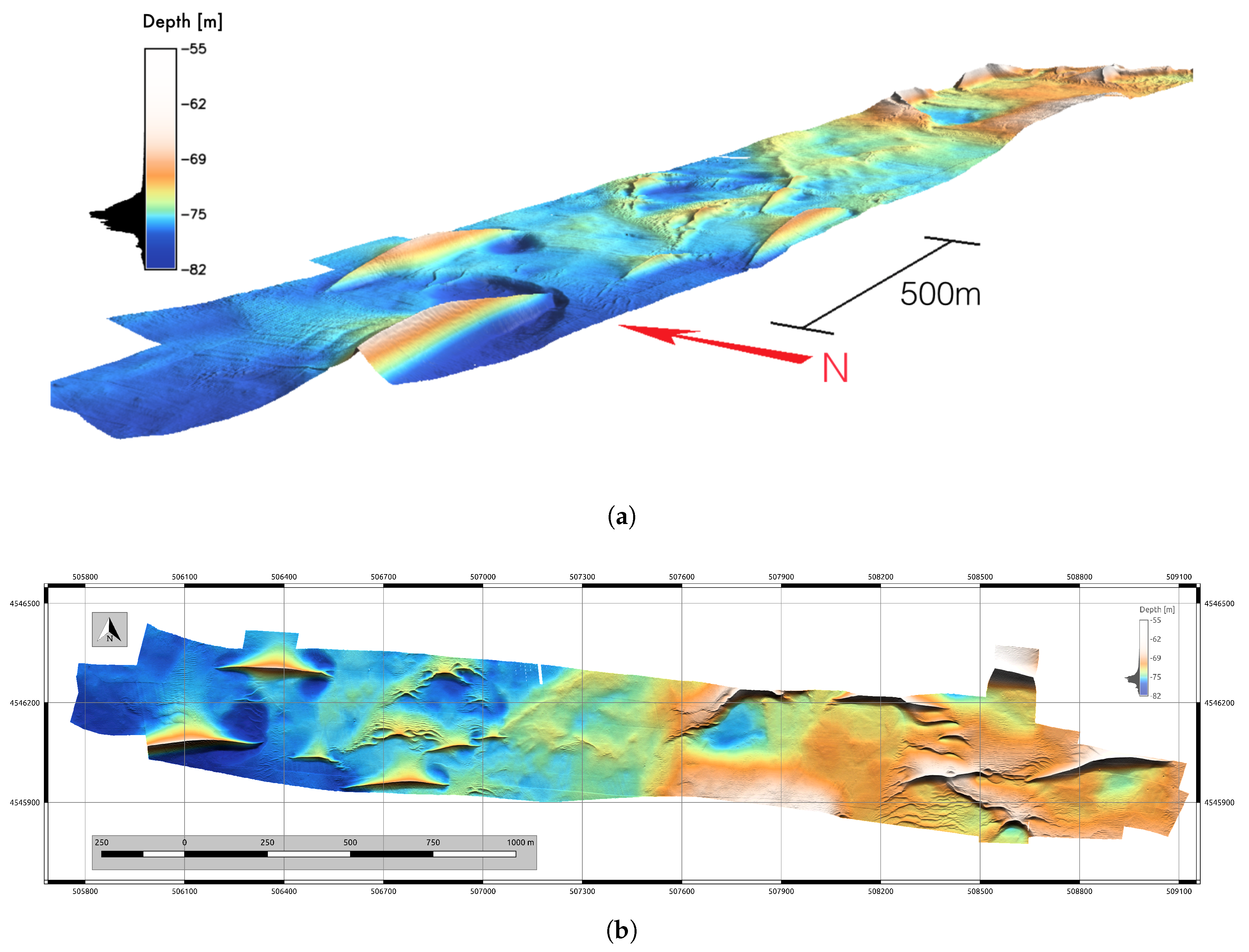
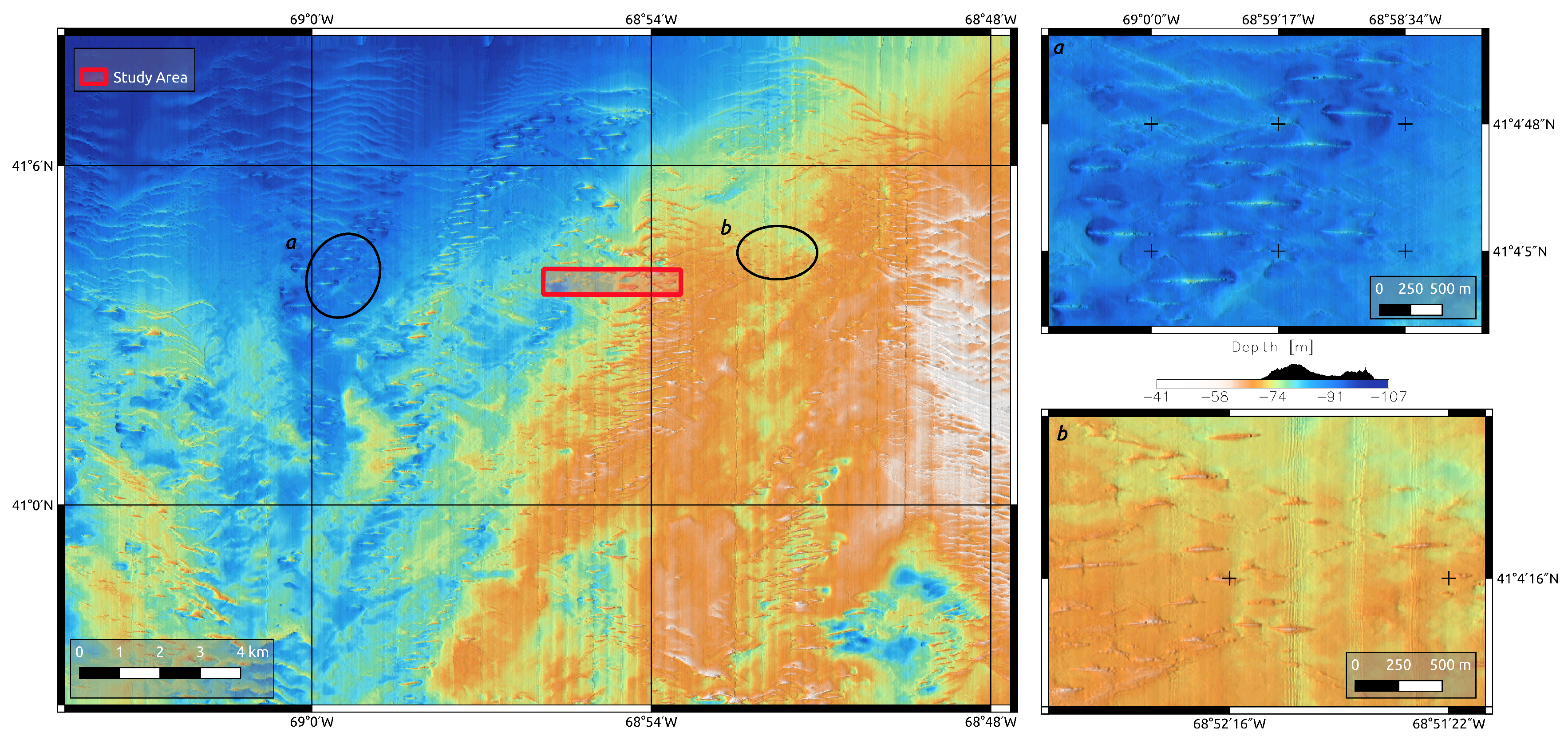
For gridding, the CUBE (Combined Uncertainty and Bathymetric Estimator) algorithm [26] was used. The CUBE settings were chosen by following the recommendations from the Field Procedures Manual, NOAA, Office of Coast Survey April 2010. The final product consisted of a bathymetric grid with a 1 m cell size (Figure 3).
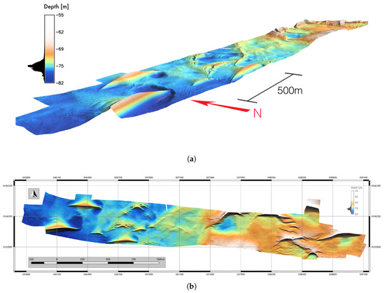
Figure 3.
Digital Bathymetry produced from the MBES data set., cell size 1 m. (a) Sout West 3D perspective, vertical exaggeration ; (b) Shaded relief, Azimuth of the sun in degrees to the east of north: , Altitude of the sun in degrees above the horizon: ; Factor for exaggerating relief: 3×.
2.3. Model Descriptions
The Spatial Analytic routine here proposed is composed of two main parts:
- Terrain Feature Extraction (TFE): Where a series of terrain parameters is computed from a digital terrain model
- Geospatial rule-based model (GRM): The identification and quantitative description of specific bedforms (e.g., sand dunes)
For the first part of the method (TFE), three different approaches for the automatic extraction of the main morphometric characteristics (terrain features) from the digital bathymetry (DBM) were compared. After evaluation of the different TFE models, the most suitable approach was determined and the outputs from this approach were used as input into the second part of the methodology (GRM).
2.3.1. Terrain Feature Extraction (TFE)
The first two approaches to feature extraction (Models Aand B) are both based on differential geometry principles [27,28,29]. In the first approach (Model A) terrain features are determined analyzing the slope and curvature of each DBM cell by running a fixed size focal window operator on the whole surface. Model A is implemented in the GRASS GIS (version: 7.3) [30] module r.param.scale which determines terrain features (namely, planar, pits, channels, pass, ridges and peaks) directly from a DBM by a single run of the model.
In the second approach, Model B, a series of terrain parameters (slope, elevation ratio and curvatures) are first extracted from the DBM and then terrain features are determined by a cell-wise unsupervised classification of these terrain parameters. The unsupervised clustering consists of two steps. First, a modified K-Means algorithm (i.cluster available in GRASS GIS) is used to group the terrain parameters into a user-specified number of clusters. Then cluster means and covariances are given as input to a maximum-likelihood discriminant analysis classifier to determine to which class each cell of the terrain has the highest probability of belonging (i.maxlik available in GRASS GIS).
A completely different approach is used in Model C which consists of applying the concept of geomorphologic phenotypes (geomorphon) [31] which is integrated into GRASS GIS. This model is based on pattern recognition principles and does not involve the derivation of terrain parameters. To determine and map landforms, the model first extracts and then labels areas characterized by a topographic pattern. Then, the pattern is compared (by matching) with a series of common landform descriptors: flat, peak, ridge, shoulder, spur, slope, hollow, foot-slope, valley, and pit [32]. For each cell, Model C performs an elevation difference between a focus pixel and pixels at a known distance (search radius) in eight principal directions (N, NE, E, SE, S, SW, W, NW). Starting from the east and proceeding counterclockwise, the algorithm produces a ternary operator which identifies a specific topographic pattern (geomorphons) that can be then associated with a particular landform element [32]. The ternary topographic pattern and associated idealized landforms are summarized in Figure 4 (e.g., example local ternary pattern is: [, 0, +1] = [lower, same height, higher]).
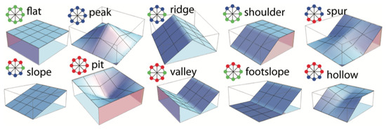
Figure 4.
Terrain features represented in r.geomorphon (J. Jasiewicz, T. Stępiński, 2012). The rose diagrams for each feature are colored based on the difference in height with the central cell as reference (green: same height, red: higher, blue: lower).
2.3.2. TFE Model Simulation
The three TFE models were evaluated and compared loosely following the evaluation framework described in “Treatise on Geomorphology: Quantitative Modeling of Geomorphology” [33]. All the models include a series of parameters that the operator can tune to control the behavior of their outputs. To investigate the scale-dependency of the TFE models and choose which model was more suitable for the detection of large-scale sand waves, a simulation experiment to analyze their sensitivity to variations in the input parameters was conducted. The list of parameters and the ranges used in the sensitivity analysis is presented in Table 1.

Table 1.
Parameters used in the sensitivity analysis of the TFE models.
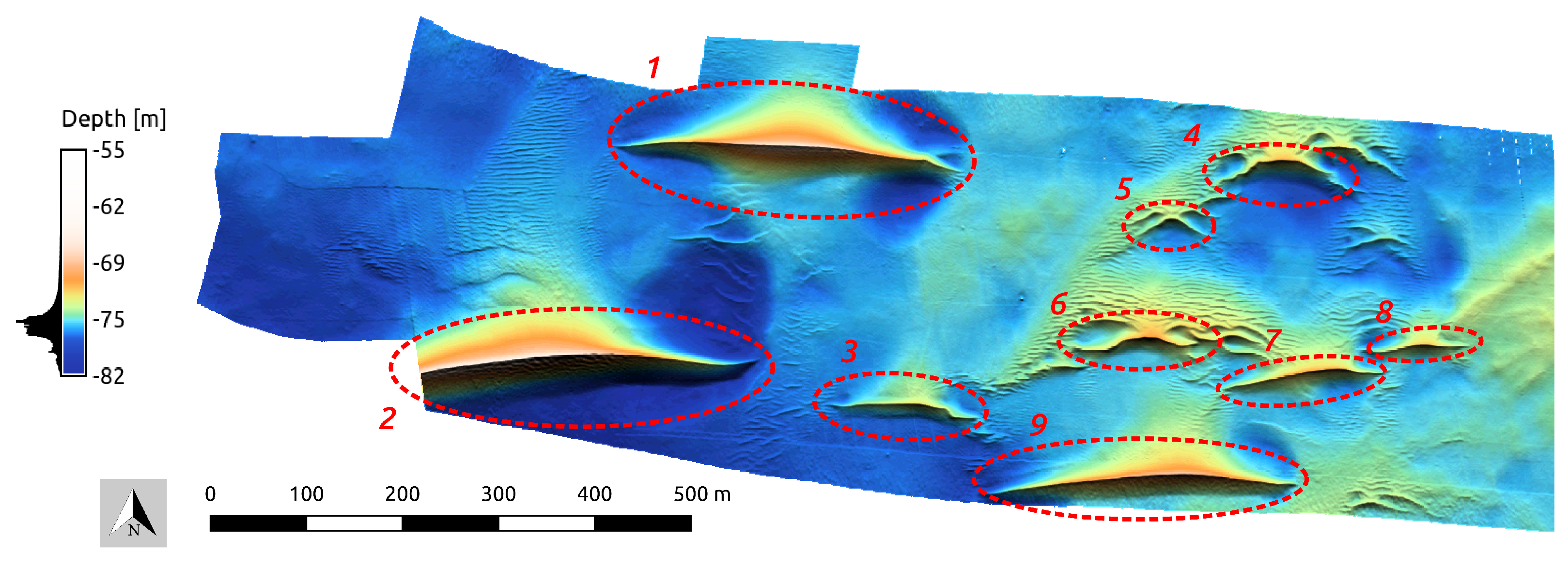
The simulation generated over 10,000 raster layers and was performed using standard consumer hardware by taking advantage of the multiprocessing capabilities of the Python programming language. It was not feasible to manually observe every single output, so a subset was selected for viewing that included the layers corresponding to the parameter combinations at the extreme and middle points of each interval. For the evaluation of the results, the outputs were compared with the desired terrain features (sand dunes) as identified visually from the DBM. When any one parameter combination returned a result that clearly matched the visually identified control features, Figure 5, the corresponding parameters were manually modified to vary around their initial values in order to see which parameter was responsible for detecting the pattern. Model C was selected as the most appropriate of the three; the reasons for this selection will be discussed in the Results section.

Figure 5.
Areas numbered 1–9 indicate visually identified sand waves with , used as control features for the selection of model outputs.
2.3.3. Geospatial Rule-Based Model-GRM
The second part of the approach is based on a Geospatial Rule-based Model (GRM) which consists of a series of geospatial processing operations, including map algebra, raster to vector conversion, topological cleaning, and, spatial filtering with the final objective of identifying and quantitatively describing a specific bedform feature, in this case large sand dunes (). The GRM is centered around the specific bedform and is applied on the output of Model C, the TFE approach that produced the best results.
The GRM rules consisted of a sequence of geospatial analysis operations implemented in two GRASS modules: r.dunes and r.dunes.metrics which are based on the output of the GRASS GIS module r.geomorphon; the entire work-flow is described in Figure 6.
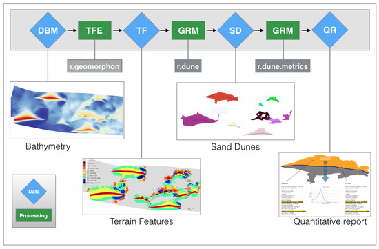
Figure 6.
Diagram describing the TFE + GRM approach for the quantitative characterization of sand dunes. The bathymetry used as input is first processed by r.geomorphon for the terrain feature extraction (TFE) and then the output is processed by the two GRASS GIS modules developed in this study: r.dune to identify sand dunes and and r.dune.metrics to produce its quantitative report.
The whole GRM workflow can be divided into three sections:
- Extract and vectorize sand wave crest (SWC).
- Extract and vectorize sand wave main body (SW).
- Identify lee and stoss side and compute sand wave’s metrics.
The sequence of each step are summarized and visually described below:
- Extract and vectorize sand wave crest for each bedform
- 1.1.
- Extraction of sand wave crest (SWC): From the TFE results (r.geomorphon), SWC are identified by extracted by reclassifying the cells with feature type equal to ridge and summit (feature type class: 2,3) into a new raster feature with category value 1 and setting the remaining cells to null (Figure 7).
 Figure 7. Extraction of sand wave crest (SWC).
 - 1.2.
- SWC thinning: SWC areas are thinned and reduced to a single pixel width (Figure 8).
 Figure 8. SWC thinning.
 - 1.3.
- SWC clumping: Each SWC is recategorized by grouping cells that form physically discrete areas into unique categories and assign a distinct color to each raster feature, different colors are assigned to each linear feature (Figure 9).
 Figure 9. SWC clumping.
 - 1.4.
- SWC filtering by length: Each feature with same category shorter than a given threshold is removed (Figure 10).
 Figure 10. SWC filtering by length.
 - 1.5.
- SWC vectorization: Conversion from raster to vector to obtain a vector feature of type line representing an approximate sand wave crest (Figure 11).
 Figure 11. SWC vectorization.
 - 1.6.
- SWC topological cleaning: Line features are cleaned by removing any dangle (Figure 12).
 Figure 12. SWC topological cleaning.
 - 1.7.
- SWC smoothing: A low pass filter is used to obtain a vectorized Sand Wave Crest (Figure 13).
 Figure 13. SWC smoothing.
- Identify areas covered by large scale bedforms
- 2.1.
- Sand wave (SW) extraction: From the TFE results (r.geomorphon), the entire landform is extracted by reclassifying the cells with feature type equal to summit, ridge, spur, and slope (feature type: class 2, 3, 5, 6) into a new raster feature with category value 1, and setting the remaining cells to null (Figure 14).
 Figure 14. Sand wave (SW) extraction.
 - 2.2.
- SW clumping: The SW raster map is recategorized by grouping cells that form physically discrete areas into unique categories and assign a distinct color to each raster feature (Figure 15).
 Figure 15. SW clumping.
 - 2.3.
- SW filtering by area: Each raster feature is reclassified based on its area, all the features having an area smaller than a given threshold are removed (Figure 16).
 Figure 16. SW filtering by area.
 - 2.4.
- SW filling: Null cells within the discrete areas are filled with the same category of the surrounding pixels (Figure 17).
 Figure 17. SW filling.
 - 2.5.
- SW vectorization: Conversion from raster to vector to obtain a vector feature of type polygon representing an approximate sand wave body (Figure 18).
 Figure 18. SW vectorization.
- Identify lee and stoss side and compute sand wave’s metrics
- 3.1.
- SW and SWC overlay: The vectorized sand wave crest is overlaid on top of the polygonal area representing the sand wave body (Figure 19).
 Figure 19. SW and SWC overlay.
 - 3.2.
- SWC clipping: The portion of the sand wave crest that is not included in the sand wave body is removed (Figure 20).
 Figure 20. SWC clipping.
 - 3.3.
- SWC buffering: A polygonal area is created by buffering the sand wave crest (buffer distance equal to the DBM cell size) (Figure 21).
 Figure 21. SWC buffering.
 - 3.4.
- SW splitting: The buffered sand wave crest is used to split the sand wave body into two parts (Figure 22).
 Figure 22. SW splitting.
 - 3.5.
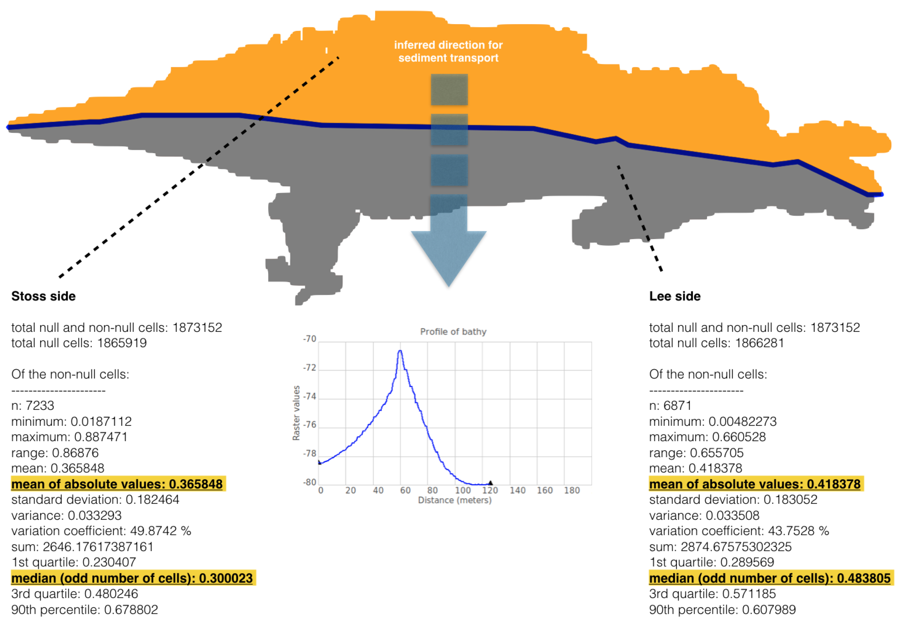
- Identification of stoss and lee side: the identification is achieved by performing an univariate statistical analysis on the DBM slope, using each sand wave side as a mask. The side with the higher values of the slope is assigned the label of lee side and is colored in grey, while the side with the lower values of the slope is assigned the label of stoss side (Figure 23).
 Figure 23. Identification of dune’s sides: stoss (colored in gray) and lee (colored in yellow).
 - 3.6.
- SW height: Derivation of SW height by generating a series of vertical profiles along several transects perpendicular to SWC. The spacing between the equidistant vertical profiles is given by an input parameter and set to as default value, the length of each profile is also variable by the user (by default is set to be the same length of the sand wave ridge) (Figure 24).
 Figure 24. SW height.
 - 3.7.
- SW width: Sand wave width (horn to horn) is obtained by calculating the distance between the endpoints of the sand wave crest.
- 3.8.
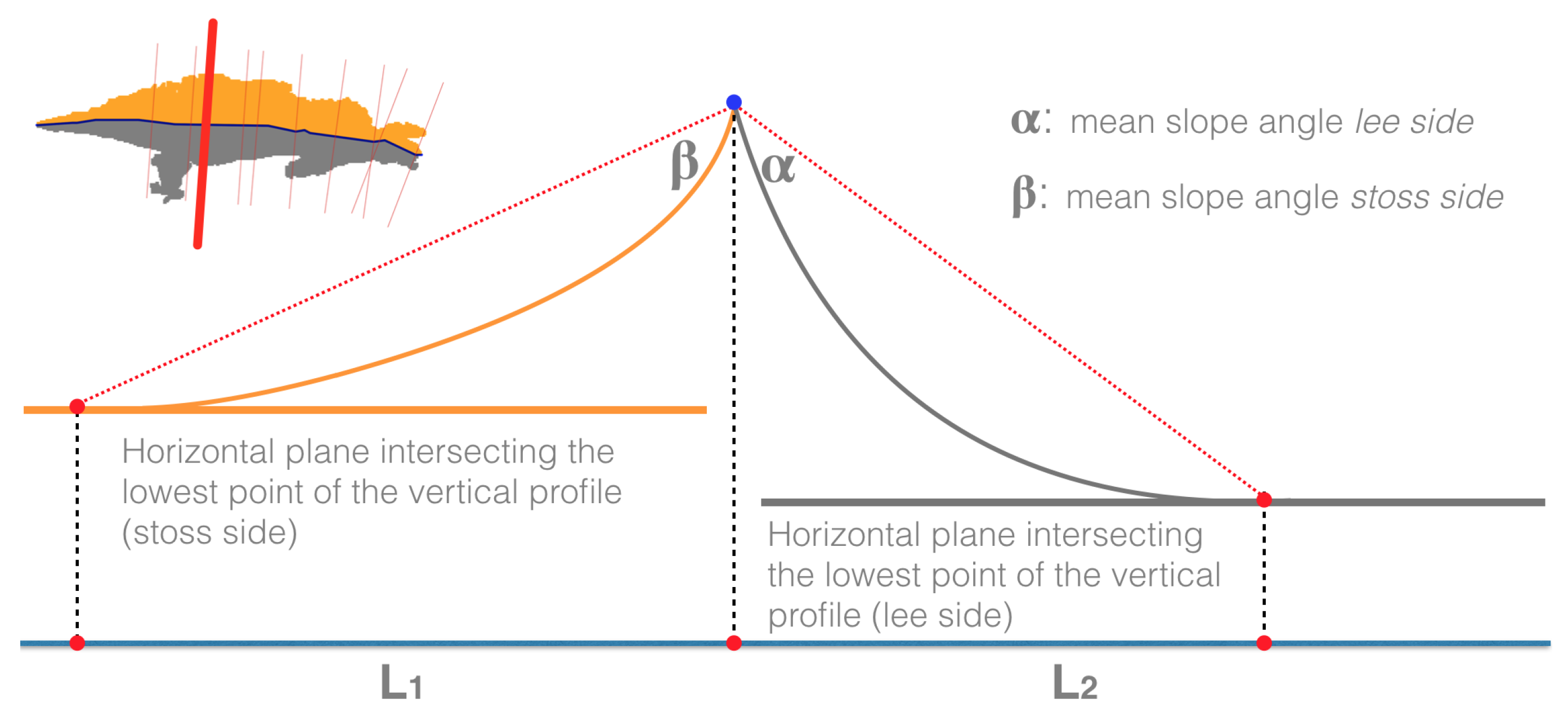
- Length: An approximate value for the length of the sand wave is obtained by following the schema in Figure 25.
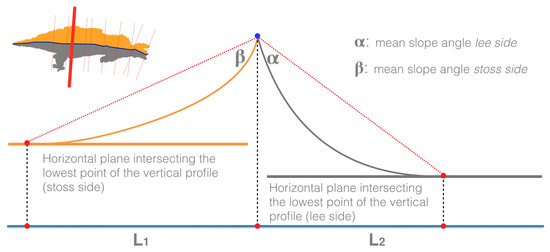 Figure 25. SW length.
Code and documentation to reproduce the whole GRM workflow are available as supplementary material.
3. Results
3.1. TFE Modeling
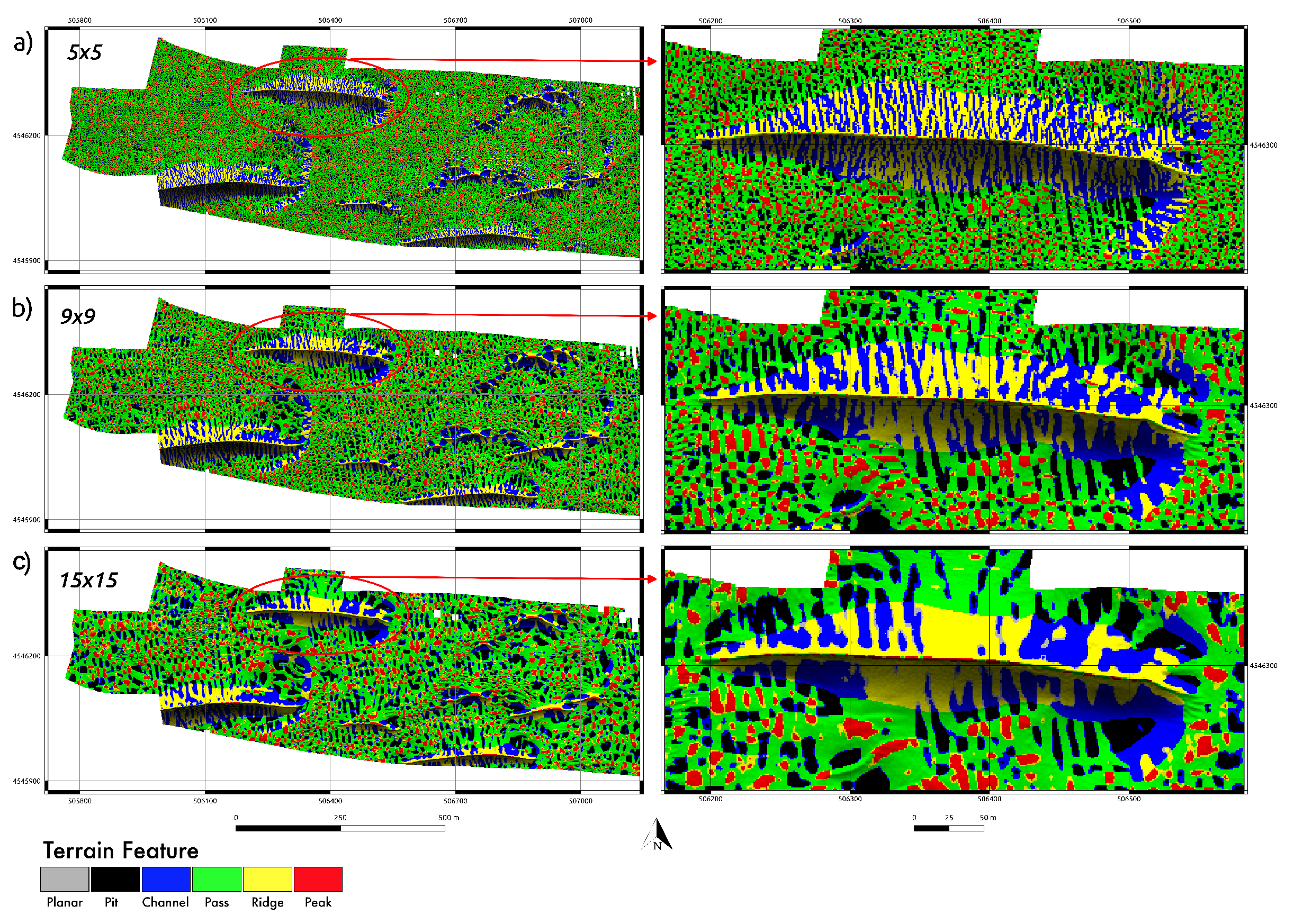
Using small values of curvature tolerance and with different window size operators, Model A easily isolated large scale features, but was not able to detect important elements of the feature like the sand wave crest (Figure 26).
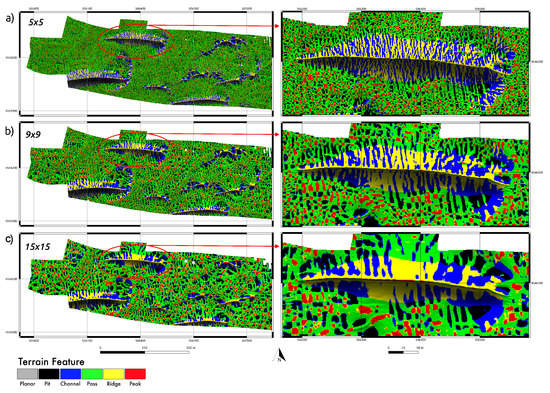
Figure 26.
Output details of Model A for small value of curvature tolerance () for different sizes (15 (a); 9 (b); and 5 (c)) of the window operator; the other parameters used were: exponent for distance weighting: 0.0; vertical scale factor: 0.5; and slope tolerance: 2.6. The zoomed areas on the right size of the image refer to the bedform labeled “1” in Figure 5.
Sand wave crests and rippled surfaces, on the other hand, could be isolated from the rest of the terrain by using relatively high values of the curvature and slope tolerance tolerance (, ), Figure 27a). Model A was also the most sensitive to artifacts in the DBM. The grid presented minor across-track artifacts (likely due to uncompensated vessel motion), which were detected as terrain features when a small () window operator were used in combination of relatively low values of curvature tolerance, () and slope tolerance, (), Figure 27b).
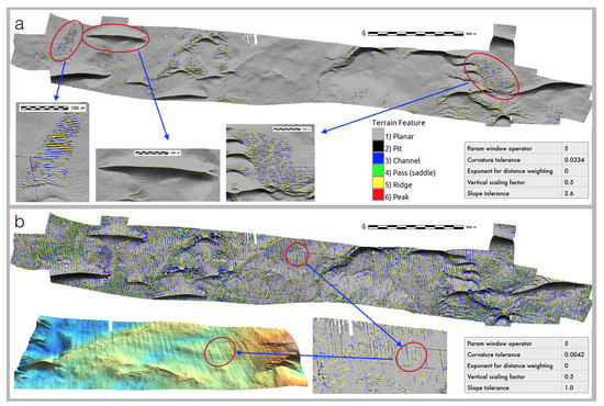
Figure 27.
Output details for Model A: (a) for high value of curvature and slope tolerance (), the model depicted rippled areas as well as dune crests; (b) for low value of curvature and slope tolerance (), the model depicted small artifact (). In (b), the 3D perspective view of the MBES dataset (vertical exaggeration: 3×) is illuminated with a light source directed from east to west (along track direction) to highlight the small () across-track artifacts likely due to uncompensated vessel motion
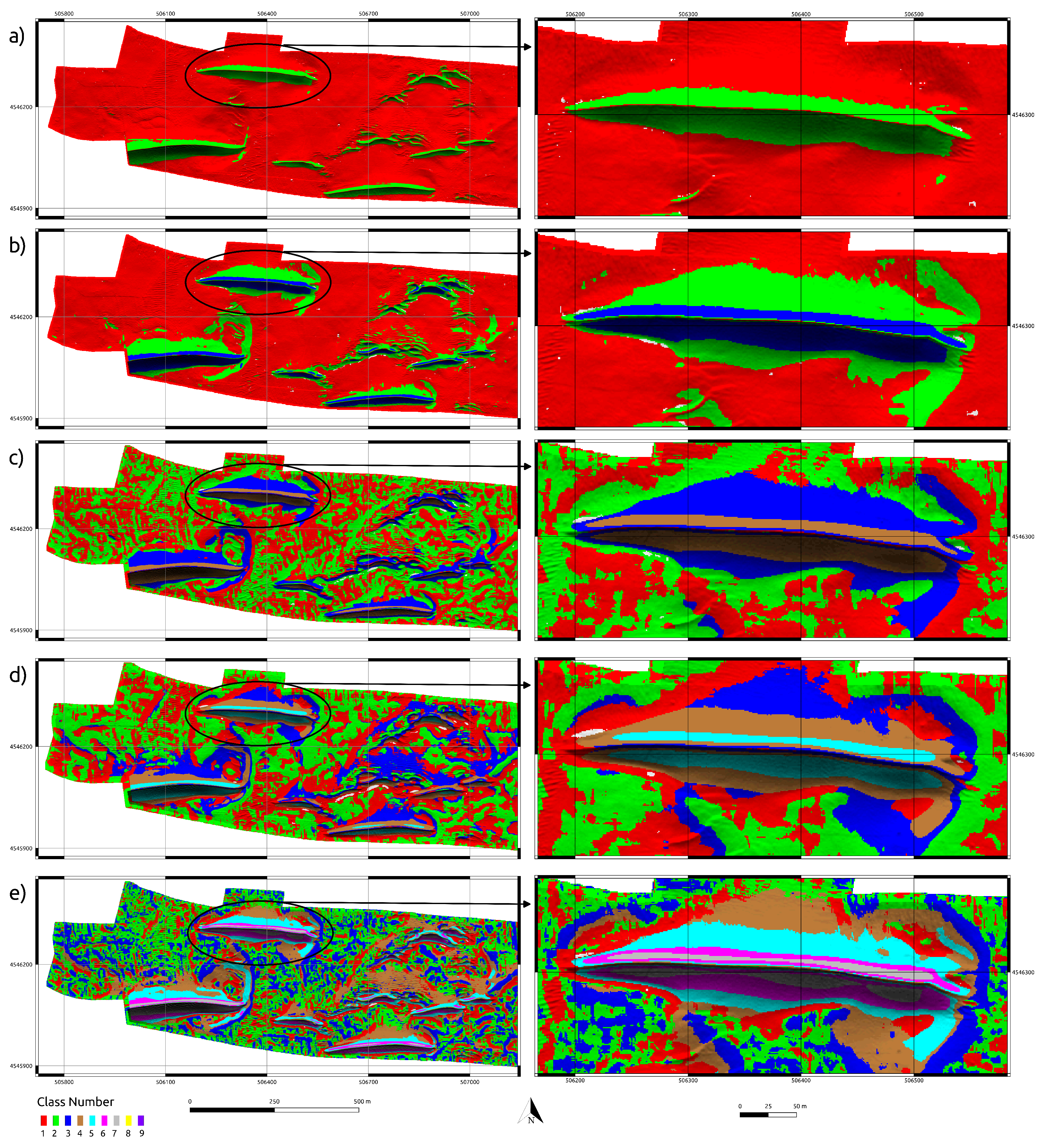
Model B results were more stable (less sensitive) to variation in the parameters used than Model A and more efficient in depicting large scale features (Figure 28). However, the inability of associating the detected feature class to specific terrain features with an established name, and the arbitrary number of user-defined classes made Model B unsuitable for the objective of this paper.
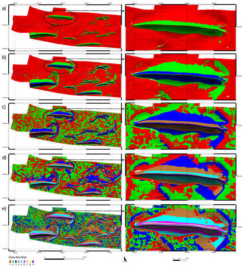
Figure 28.
Output details for Model B: (a) three classes, window operator cells; (b) five classes, window operator cells; (c) five classes, window operator cells; (d) seven classes, window operator cells; and (e) nine classes, window operator cells. The other parameter are kept constant: slope tolerance (), curvature tolerance (), and vertical scale factor (). Each color represent a different class. The zoomed area on the right of each panel refer to the bedform labeled “1" in Figure 5.
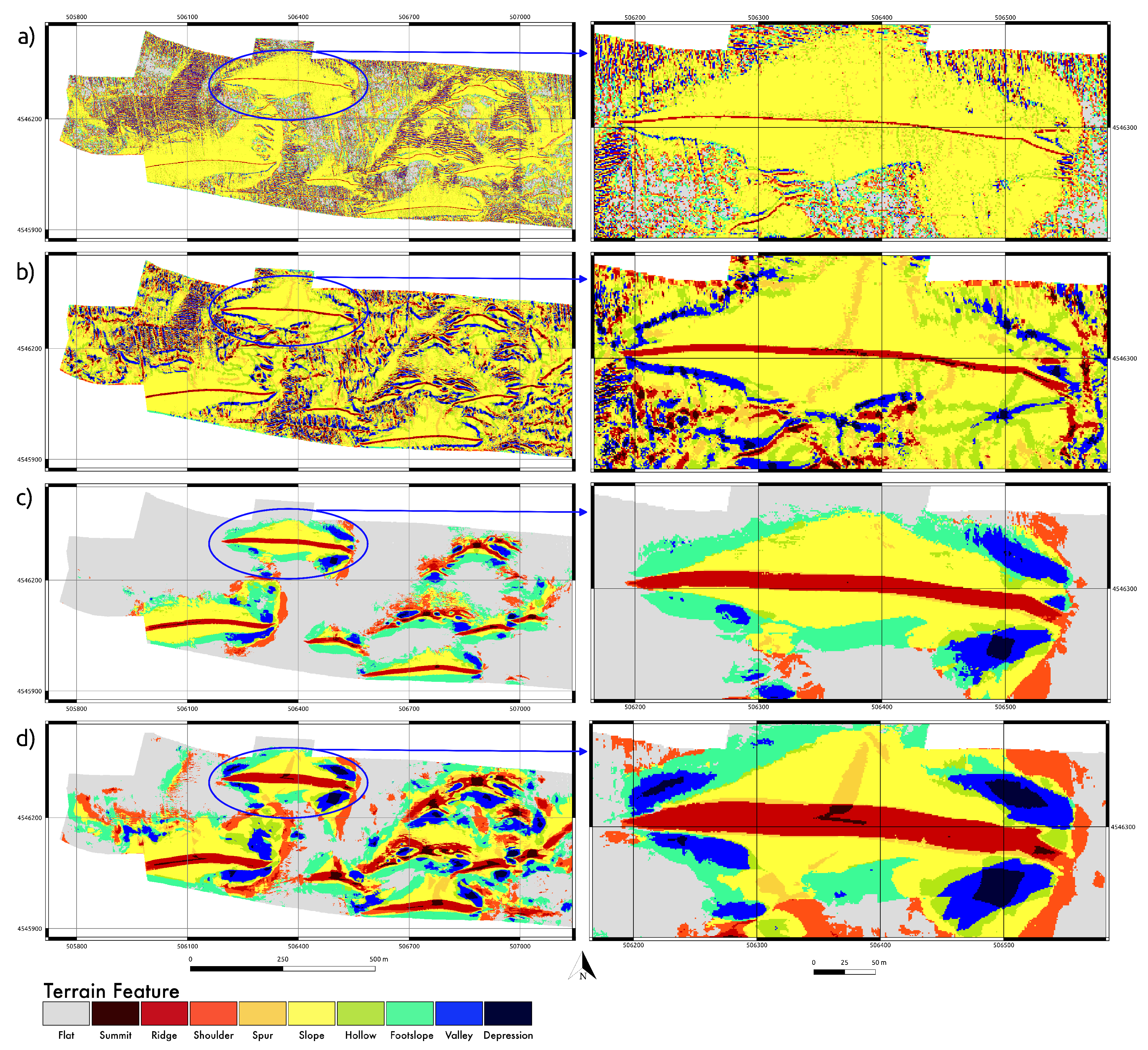
The r.geomorphon approach (Model C) outperformed the methods based on differential geometry. It was able to depict important landform elements at different scales with a single run of the model. Model C presented the most stable results, particularly when the search radius parameter reaches values greater than 30 cells. For almost all combination of parameters, Model C was able to correctly depict all sand wave crests, a key element for sand waves characterization (Figure 29).
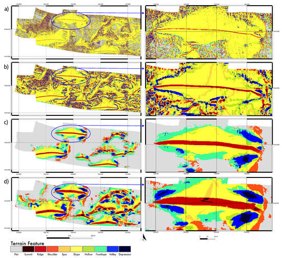
Figure 29.
Output details for Model C, r.geomorphon: (a) r.geomorphon default values, outer search radius: 3, inner search radius: 0, flatness threshold: 1, flatness distance: 0; (b) outer search radius: 11, inner search radius: 3, flatness threshold: 0.1, flatness distance: 0; (c) values chosen to implement the GRM model: outer search radius: 35, inner search radius: 9, flatness threshold: 3.7, flatness distance: 15; and (d) outer search radius: 45, inner search radius: 19, flatness threshold:1, flatness distance: 15. The zoomed area on the right of each panel refer to the bedform labeled “1” in Figure 5.
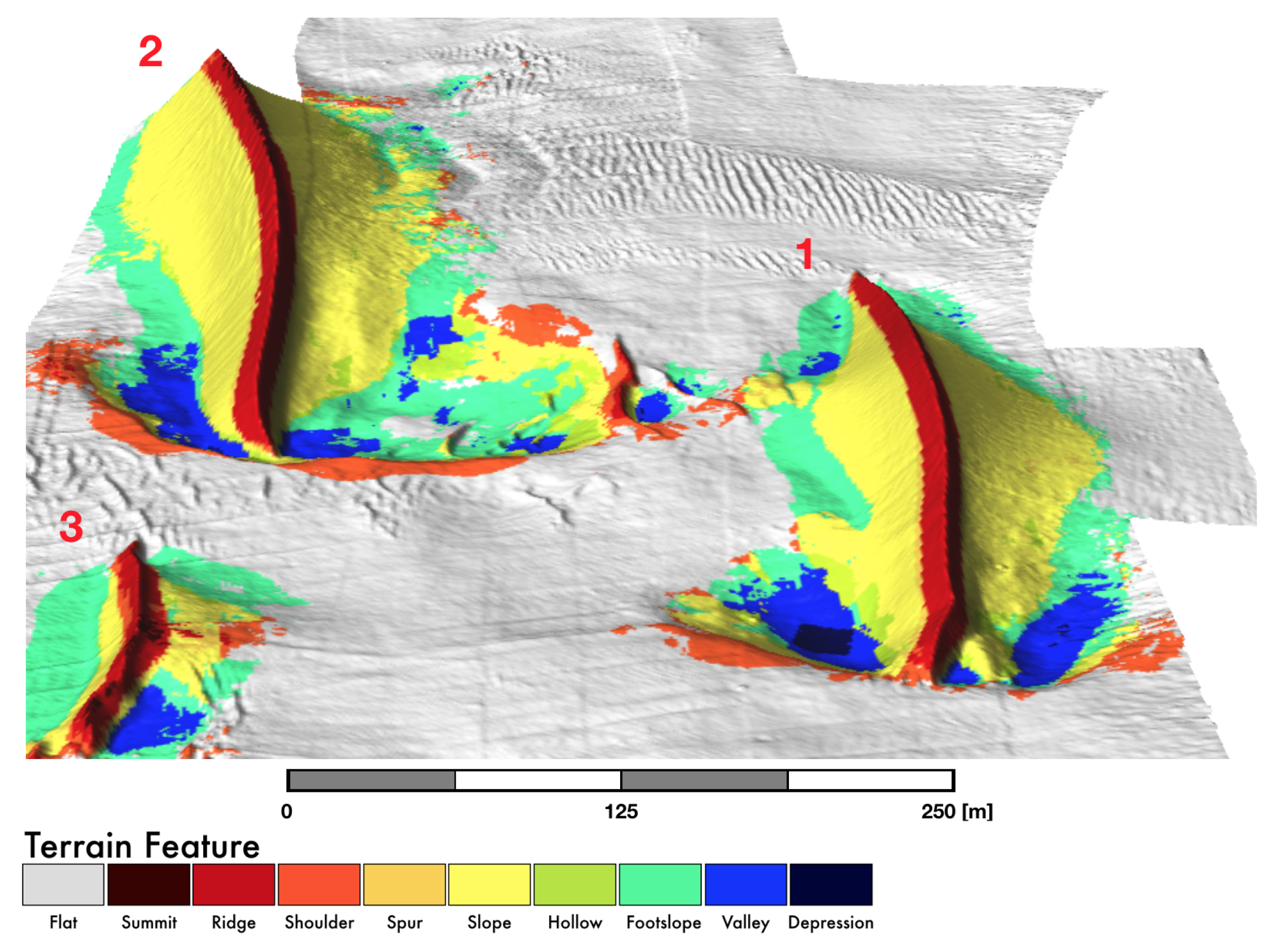
The simulation thus showed that, for a particular range of parameters, all three models were able to detect some of the terrain features that could be associated to a specific landform (e.g., isolated crest for sand dunes, concave surface for depressions and patterns of almost parallel slope–ridge–valley in the case of sand ripples) but none could do so in a single run. In particular, Models A and B returned very different results for different input parameters showing a greater sensitivity to parameter changes and thus a greater scale-dependency. Model B results were more stable (less sensitive) to variation in input parameters and most efficient in depicting large scale features, however the lack of an exact labeling for the detected features and the arbitrary number of user-defined classes made the model unsuitable for the objective of this study. Model C produced the most stable outputs particularly when the size of the search radius was 30 cells or more, confirming the scale-flexibility of the model [32]. Thus, Model C was chosen as the most appropriate for extracting the desired bedform feature, in this case large sand dunes; output for the chosen set of parameters is shown in Figure 30.

Figure 30.
Details of Model C outputs (r.geomorphon: outer search radius: 35, inner search radius: 9, flatness threshold: 3.7, flatness distance: 15), draped on top of the DBM, (vertical exaggeration: 3×). The numbers on the top left of each bedform refers to the “bedforms labeled 1, 2, and 3” in Figure 5.
3.2. GRM Modeling
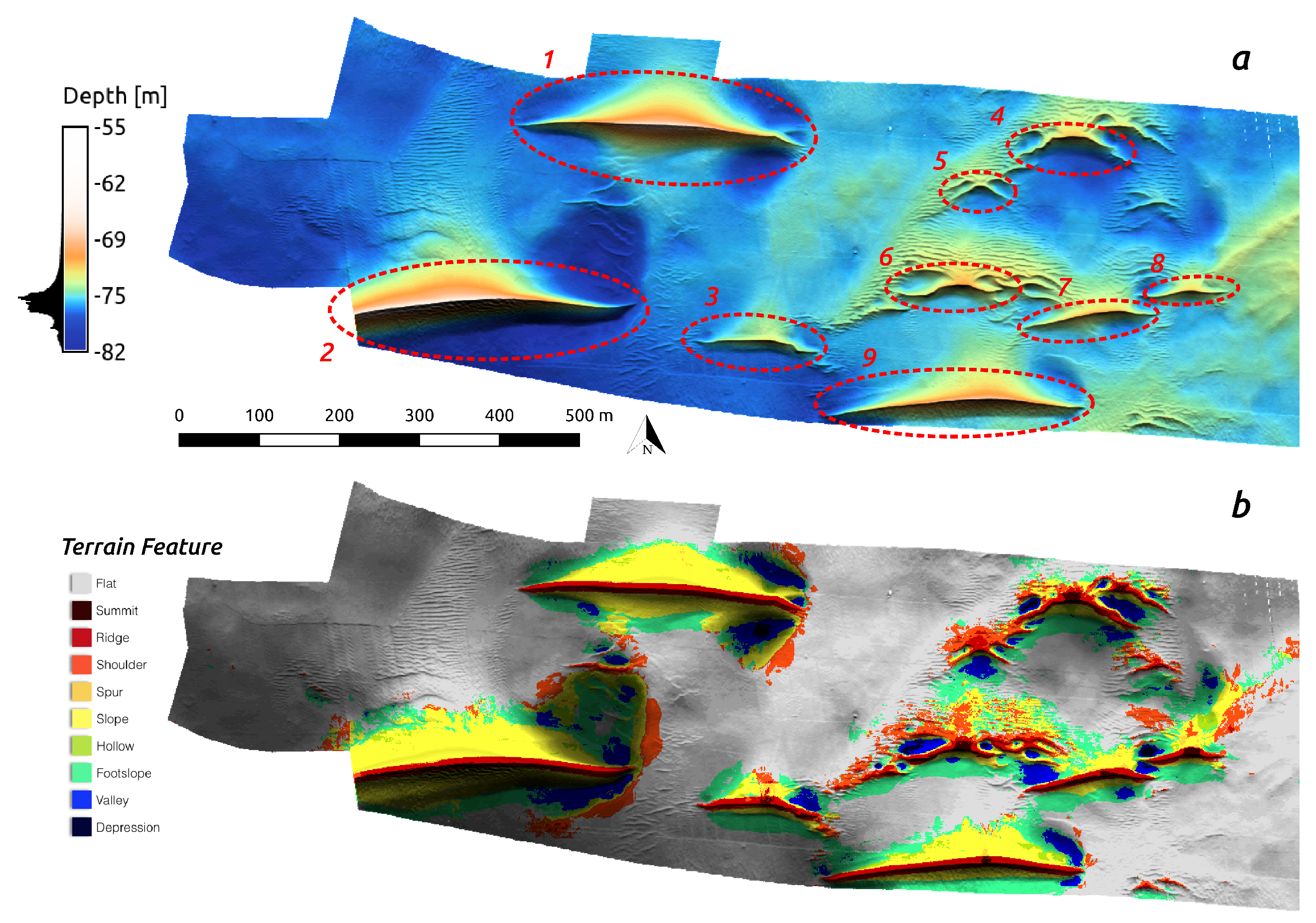
Having selected the most robust approach for feature identification, the rest of the analysis focuses on developing a GRM routine that uses the output of Model C to automatically characterize large () sand waves. A single run of Model C with the appropriate combination of its parameters was able to correctly depict most of the control features chosen to test the models in this paper (Figure 31).

Figure 31.
Control units (a); and Model C outputs (b), r.geomorphon parameters used: : 35, : 9, : 3.7, : 15. Color images draped over a shaded relief (azimuth of the sun in degrees to the east of north: , altitude of the sun in degrees above the horizon: ).
The model developed in this paper has been implemented in two GRASS GIS modules, (r.dune) and r.dune.metrics. In r.dune, the output of the TFE model (r.geomorphon) is used as input to extract the sand wave and return a vector layer with two features: (1) a polygonal feature representing the area of the bedform; and (2) a line feature that identifies the sand wave crest. In r.dune.metrics, the output of r.dune is used to query the original DBM and generate a quantitative report for each sand dune. The metrics computed by the module include: length, width, height, vertical profile, identification of stoss and lee side, and slope statistics for each side. The module outputs are summarized in a PDF report for each bedform (Figure 32).
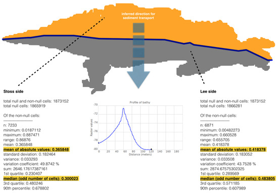
Figure 32.
Bedform report, output of r.dune. The different colors indicate the stoss (yellow) and lee (gray) sides of the bedform. The tool runs a number of vertical profiles along transects perpendicular to the dune crest (blue). The spacing between transects is controlled by a parameter set (by default) to the DBM cell size in meters, same for the length of the transect which is (by default) set to be equal to the sand crest length (in meters). The vertical profile chosen for the report is the one with the greatest (or maximum) difference in depth.
A report with the main metrics (Length, Width, and Height) for all the bedforms identified is also available as output.
4. Discussion
Quantitative characterization of bedforms can provide a valuable source of information for a number of areas of science and engineering. Engineering applications include sediment transport studies and estimates of sand resource volumes. For ecologists, such a quantitative description can be useful in developing species distribution models by helping to test the hypothesis that morphology has a direct influence on the spatial distribution of benthic species and by relating the distribution of marine life with scale-dependent landforms.
By automatically identifying the areas where specific landforms are located, it is possible to rapidly: (1) compute the extent of those landforms in an objective and reproducible way; and (2) perform a stratified sampling of ecological information (e.g., high-resolution seafloor images, physical samples, etc.) by selecting only samples falling within a specific geomorphic category which will facilitate the definition of biotopes (by annotating species diversity, abundance, etc.) associated with a specific geomorphic category.
The three models presented have both advantages and disadvantages. Model B, by the nature of the unsupervised classification method adopted, needed an a priori number of classes, each of which was assigned a dummy label. Although it is possible to tune the number of final clusters so that they are statistically acceptable by varying the class separation parameter in i.cluster, their labels are still arbitrarily assigned. In contrast, Models A and C assign a specific geomorphological feature label to each object extracted.
A positive aspect of Model B is the ability to accept an undefined number of predictor variables as input (in addition to the terrain derivatives). This last characteristic can be of particular interest when the area of the analysis spans across very different sediment types, which are known to characterize different biotopes [34]. In this case, Model B can take advantage of the valuable information that can be provided by adding acoustic backscatter from MBES as input to the model.
It was observed that, by combining the results of multiple runs of each model using different values of the input parameters, it was possible to identify bedforms at more than one scale in a given area. For example, by identifying and masking out flat areas and large-scale features, and using a high value for the curvature tolerance, Model A performed very well in depicting rippled areas (Figure 10a). This behavior of the models confirms their scale-dependency and validates the idea that a unique and objective terrain classification framework is not easily achieved [29].
As shown in Figure 31, Model C was able to identify large-scale features correctly. In particular, the area covered by each landform was successfully identified and the ridge of each sand wave was correctly depicted. By using these two features, and by knowing the particular label associated with each class, a reclassification routine is enabled for the further quantitative characterization of the bedform.
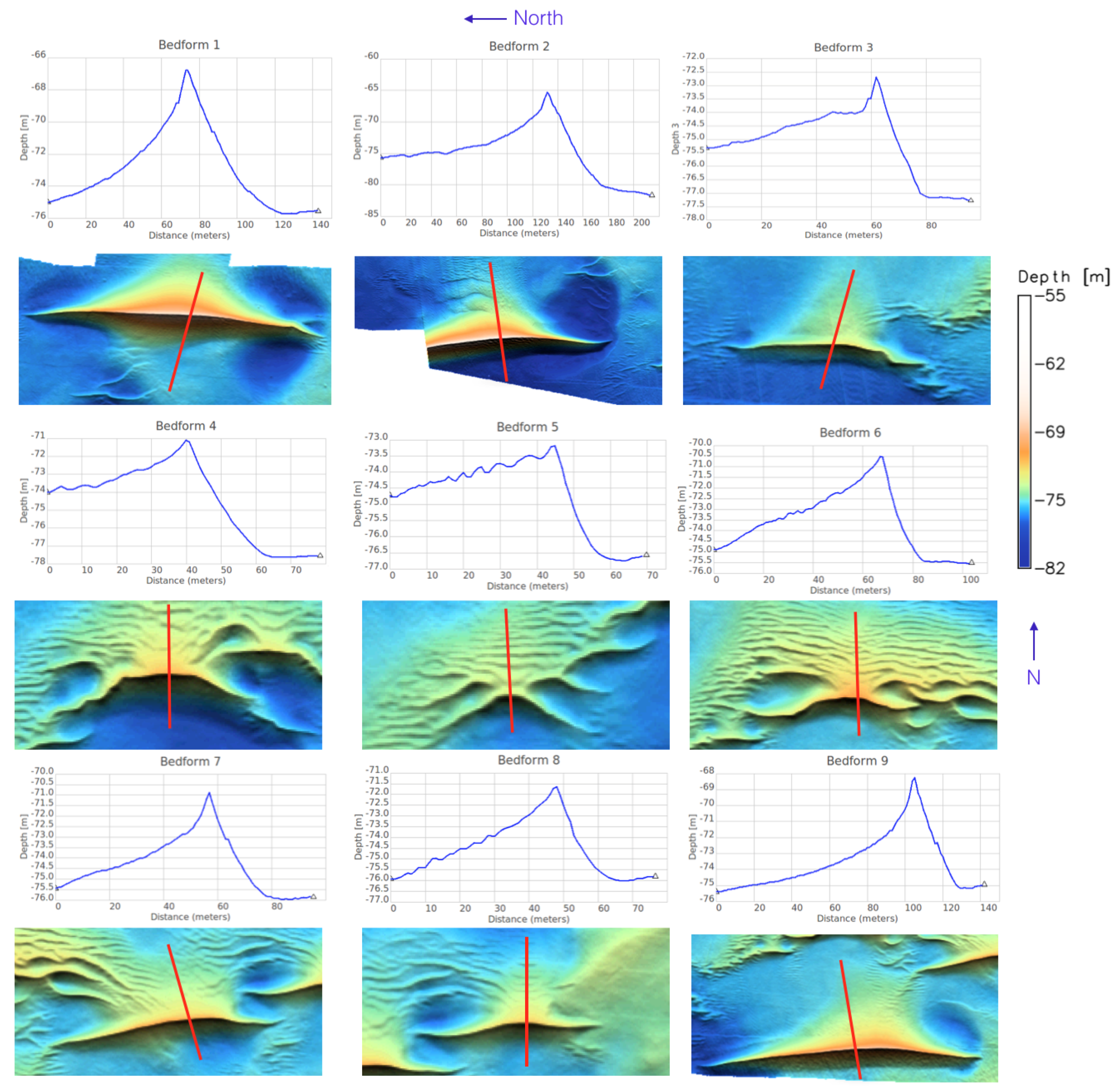
Once the sand dunes were identified, the GRM approach was used to analyze the asymmetry of the dunes, which in turn can provide evidence of flow direction and speed as well as overall seafloor energy conditions. The dunes mapped in this study were very asymmetric (Figure 33), suggesting that they are mobile [35].
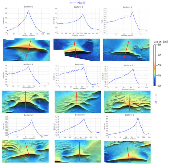
Figure 33.
Vertical profiles for the sand waves identified by the r.dune module.
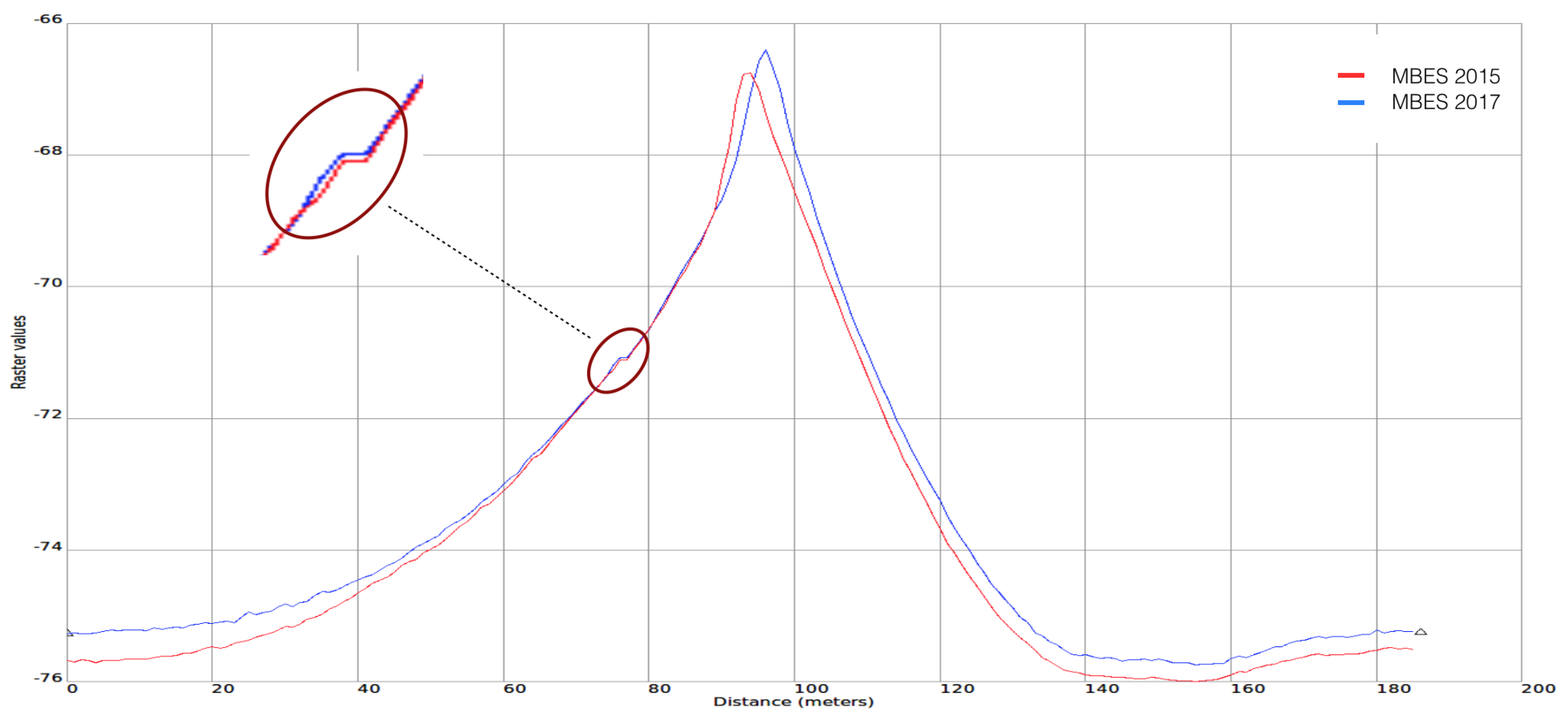
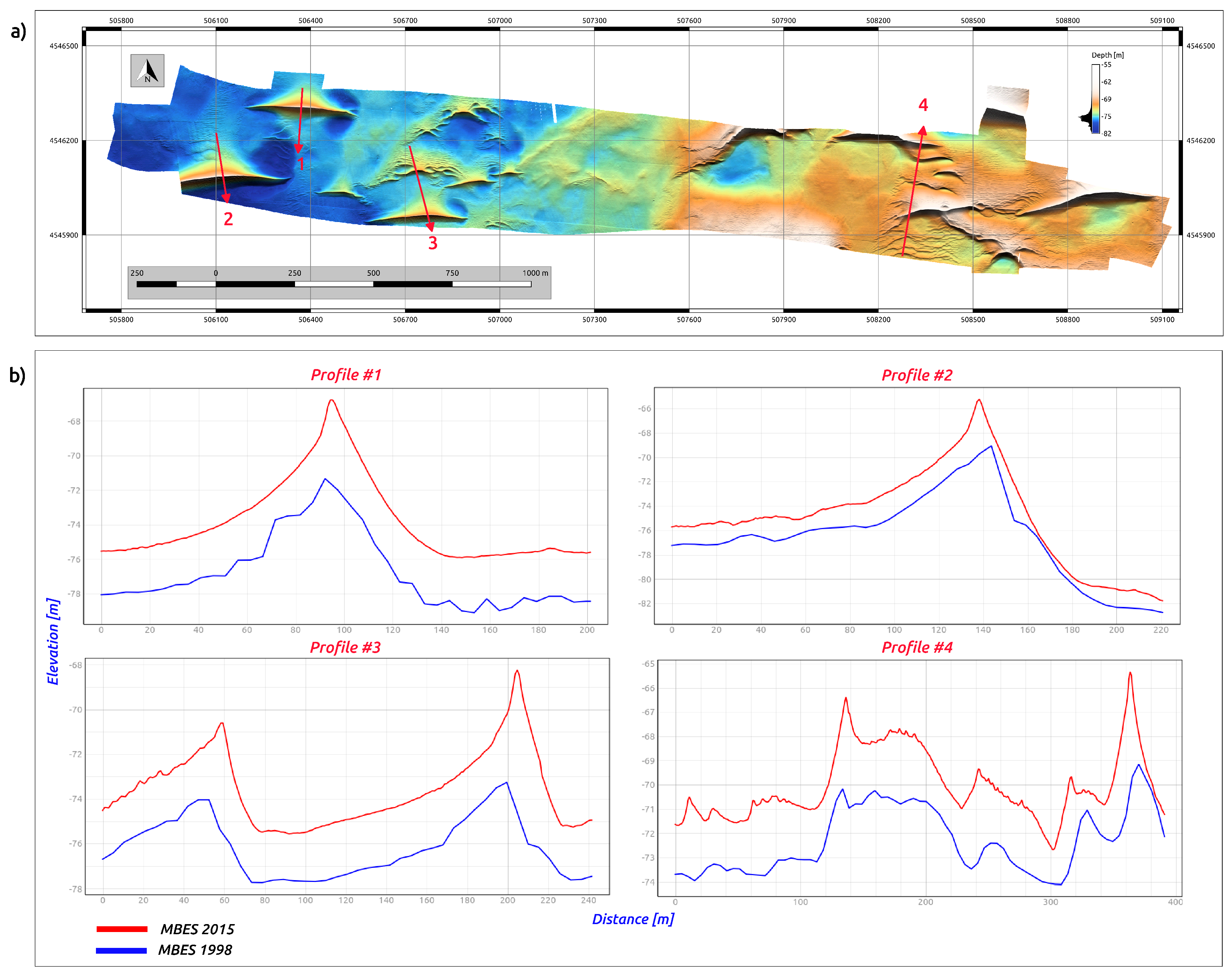
However, in 2017, a new MBES dataset was collected over the same area, which showed the dunes in the same location with an almost identical vertical profile (Figure 34), thus implying that their crests have not migrated over the two-year period. Furthermore, MBES data from 1998 [23] were also available and compared to the dataset used in this paper, confirming that indeed these bedforms have not migrated (Figure 35b).
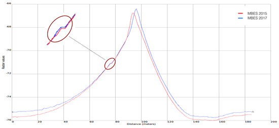
Figure 34.
Vertical profile for one of the sand dunes from two different cruises, data collected in 2015 (red) and 2017 (blue). From the zoomed details, on the upper half of the stoss slope, a horizontal step is visible that matches almost perfectly between the two datasets.
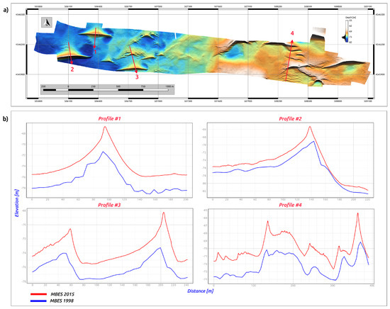
Figure 35.
Vertical profiles (a, b) comparing the two MBES dataset collected in 1998 (blue, cell size: 9m), and 2015 (red, cell size: 1m). Lines numbered 1–4 in (a) indicate the transect used to plot the vertical profiles in (b). A constant vertical offset of about can be seen, attributed to differences in accuracy and resolution of the data acquisition systems used in the two cruises.
From the vertical profiles, it is also possible to observe small differences on the east side of the survey area which is probably due to a larger amount of soft sediment, as can be seen from the acoustic backscatter (BS) collected during the 1998 MBES survey (Figure 36).

Figure 36.
Acoustic Backscatter (BS) collected in 1998 (Simrad Subsea EM 1000 Multibeam Echo Sounder, 95 kHz), dark area low BS. Lines numbered 1–4 indicate the transects used to plot the vertical profiles in Figure 35)
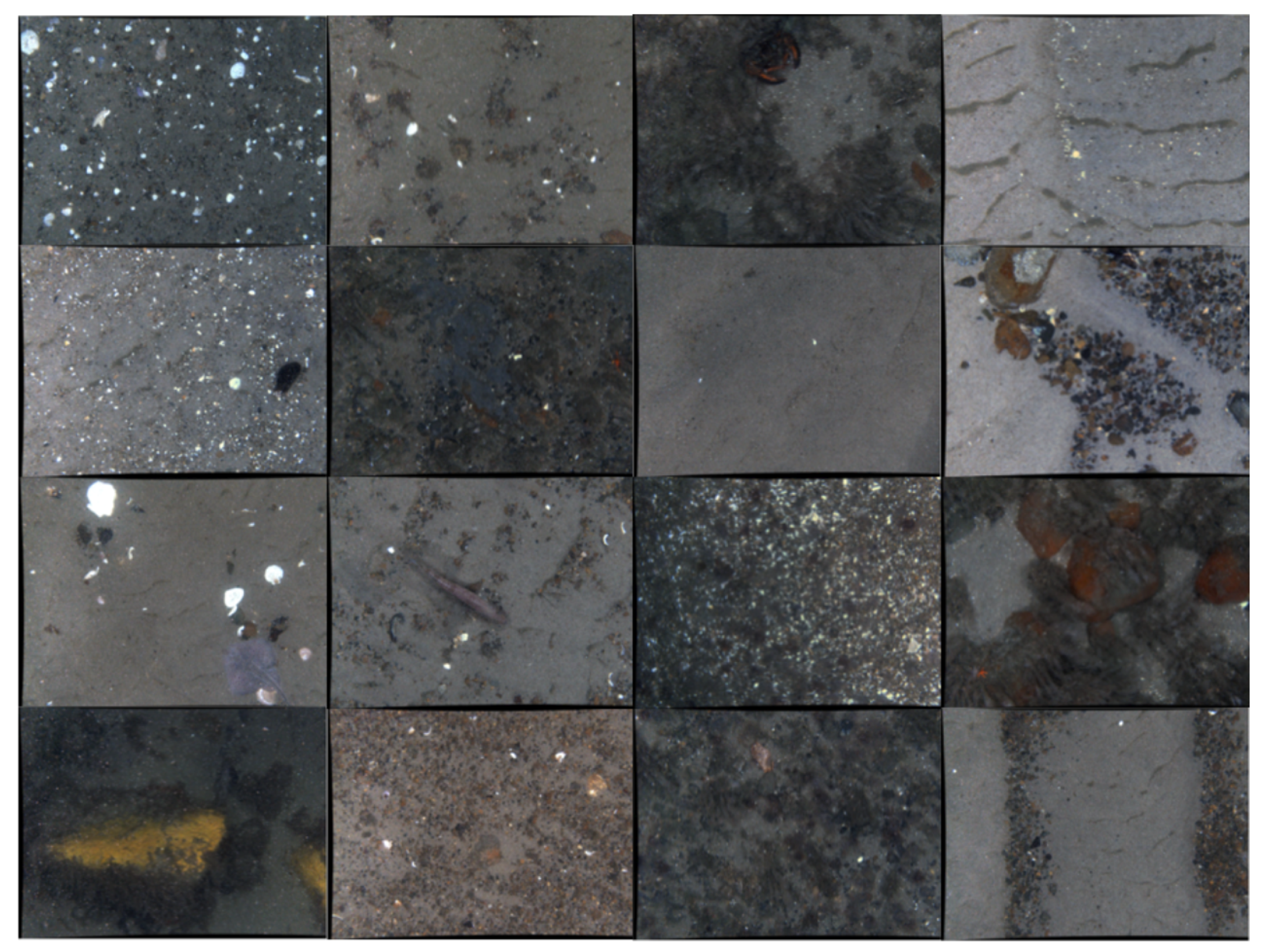
The methods developed here enable the automatic identification and quantification of isolated sand dunes. This allows these bedforms to be rapidly identified, mapped and characterized over large areas, providing valuable information on the distribution and transport of sediment and more generally seabed energy conditions. The method can be easily extended to include other bedforms such as sand ripples and mega-ripples. Moreover, with the development of additional bedform metrics, the GRM method developed here has the potential to further allow the classification of dunes into their types (e.g., barchans versus `whaleback’ dunes). Direct applications of this work extend to the field of ecological science and habitat mapping. For example, in the area described in this study, the HabCam imagery showed a heterogeneous seafloor comprising multiple biotopes (Figure 37).
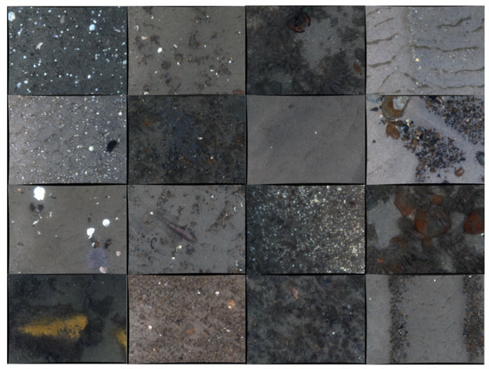
Figure 37.
A selection of HabCam images collected during the 2015 MBES survey that indicate the presence of different biotopes surrounding the bedforms area. Each image covers an area of approximatively .
Given the ability to objectively and consistently define bedform boundaries, it becomes possible to collect habitat information from within (or outside of) these areas and thus relate biotopes and bedforms at various scales. In particular, it will be possible to study habitat patchiness by looking at the correlation, if any, of a particular biotope and its relative position, size and distance from bedforms of a particular type and scale. The isolated bedform objects of this study are a representative feature of the Great South Channel (see Figure 38). The habitat information derived by analyzing the high resolution MBES and imagery dataset can thus be used to extrapolate habitat information over a much wider area where similar “seascape ecological units” can be identified.
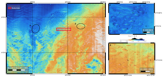
Figure 38.
Portion of the USGS bathymetry collected in 1998 [23]. The isolated bedforms object of this study are a representative feature of the Great South Channel seabed. The zoomed areas (a,b) show in detail two, of many, areas where it is possible to find isolated dunes.
The adoption of the geomorphon concept in combination with the scripting flexibility of GRASS GIS allows the development of complex and effective GRM routines thus offering a complete platform for automatically detecting a wide range of bedforms. A simple extension to the GRM model presented in this work, is to implement dune classification by type, e.g., barchans vs. whaleback, by computing the planar ray of curvature of the sand wave crest. More complex GRM models can also be implemented for other types of bedforms. By choosing the appropriate TFE model and by tuning its input parameters, it is possible to implement the detection and characterization of other types of bedforms, e.g., rippled areas. For example, using a high value of curvature and slope tolerance (Figure 27a) in the TFE Model A, rippled areas are clearly depicted. One approach to extract the rippled areas for their further quantitative characterization would be to:
- Set to null all the regions occupied by large scale bedforms and all the planar feature class.
- Vectorize channel and pass feature classes as vector lines.
- Split the vector lines into equidistant points.
- Determine the area occupied by ripples by using a kernel density estimator.
In this way, it is possible to map rippled areas and further develop the model for their allometric characterization (amplitude, wavelength etc.).
5. Conclusions
This study used acoustic data to develop a technique for the quantitative characterization of bedforms. Three models for the extraction of terrain features from a DBM were considered and evaluated in a simulation experiment to study their sensitivity to a range of input parameters including scale dependence. Simulation results were used as a guide to choose a set of parameters more suitable for the extraction of particular scale-dependent terrain features, namely large isolated sand dunes.
From the simulation results, it was shown that, for different parameters, all models were able to accurately depict different terrain features. Such behavior is an indicator that there is no best model, but a combination of them will usually be necessary to achieve a complete multi-scale, quantitative, morphometric characterization of bedforms.
This experiment provided an efficient way to address the scale dependency of digital terrain analysis, enabling the classification of specific landforms by developing ad-hoc (landform/scale specific) reclassification routines. Although only sand waves were considered here, this approach can be readily used in combination with pattern-based geospatial analysis to identify other scale-dependent bedforms, like sand ripples. Through pattern-based geospatial analysis of categorical raster maps, including those generated by TFE models, patterns of terrain features can be defined. These can then be used to identify a given bedform type which in turn can be quantified by the implementation of a GRM model.
The procedure presented here marks a step forward towards the adoption and automation of specific morphometry techniques for the quantitative characterization of bedforms.
Supplementary Materials
Code and documentation to reporoduce the results presented in this paper are available at: https://doi.org/10.5281/zenodo.1149563.
Acknowledgments
The survey data were collected during the 2015 NOAA annual federal Sea Scallop Survey on board R/V Hugh Sharp, operated by the University of Delaware, and funded by the Improve a Stock Assessment Program of the NOAA Northeast National Marine Fisheries Service (NEMFS). The authors would like to thank Burton Shank, for his invaluable help in the survey planning and as facilitator with the other co-PI who generously granted vessel time for data acquisition, James V. Gardner, for his scientific guidance and support, and Richard P. Signell and Page C. Valentine for providing useful insights about the study area. This work was supported by NOAA GRANT NA15NOS400002000.
Author Contributions
Massimo Di Stefano conceived and designed the experiments, conducted the field research and did most of the analysis and manuscript. Larry Mayer discussed concepts and approaches and contributed to the writing of the manuscript.
Conflicts of Interest
The authors declare no conflict of interest.
Abbreviations
The following abbreviations are used in this manuscript:
| DEM | Digital Elevation Model |
| DBM | Digital Batimetry |
| DTM | Digital Terrain Model |
| DTA | Digital Terrain Analysis |
| TPE | Terrain Parameters Extraction |
| TFE | Terrain Feature Extraction |
| MBES | Multibeam Echocouder |
| CTD | Conductivity, Temperature, Depth |
| USBL | Ultra Short Baseline |
| R/V | Research Vessel |
| IMU | Inertial Measurement Unit |
| GPS | Global Positioning System |
| GIS | Geographic Information System |
| GRASS | Geographic Resource Analysis Support System |
| SW | Sand Wave |
| SWC | Sand Wave Crest |
| CCOM | Center For Coastal and Ocean Mapping |
| WHOI | Woods Hole Oceanographic Institution |
| USGS | United States Geological Survey |
| NOAA | National Oceanic and Atmospheric Administration |
| NEMFS | North East Marine Fisheries Center |
| CMECS | Coastal and Marine Ecological Classification Standard |
References
- Kruckeberg, A.R. Geology and Plant Life: The Effects of Landforms and Rock Types on Plants; University of Washington Press: Seattle, WA, USA, 2002. [Google Scholar]
- Porder, S. Coevolution of life and landscapes. Proc. Natl. Acad. Sci. USA 2014, 111, 3207–3208. [Google Scholar] [CrossRef] [PubMed]
- Odum, E.P.; Kroodsma, R.L. Fundamentals of Ecology; Saunders: Philadelphia, PA, USA, 1976. [Google Scholar]
- Harris, P.T.; Baker, E.K. Seafloor Geomorphology as Benthic Habitat; Elsevier: Amsterdam, The Netherlands, 2011; pp. 3–22. [Google Scholar]
- McArthur, M.A.; Brooke, B.P.; Przeslawski, R.; Ryan, D.A.; Lucieer, V.L.; Nichol, S.; McCallum, A.W.; Mellin, C.; Cresswell, I.D.; Radke, L.C. On the use of abiotic surrogates to describe marine benthic biodiversity. Estuar. Coast. Shelf Sci. 2010, 88, 21–32. [Google Scholar] [CrossRef]
- Lecours, V.; Devillers, R.; Simms, A.E.; Lucieer, V.L.; Brown, C.J. Towards a framework for terrain attribute selection in environmental studies. Environ. Model. Softw. 2017, 89, 19–30. [Google Scholar] [CrossRef]
- Che Hasan, R.; Ierodiaconou, D.; Laurenson, L.; Schimel, A. Integrating Multibeam Backscatter Angular Response, Mosaic and Bathymetry Data for Benthic Habitat Mapping. PLoS ONE 2014, 9, e97339. [Google Scholar] [CrossRef] [PubMed]
- Brown, C.J.; Smith, S.J.; Lawton, P.; Anderson, J.T. Benthic habitat mapping: A review of progress towards improved understanding of the spatial ecology of the seafloor using acoustic techniques. Estuar. Coast. Shelf Sci. 2011, 92, 502–520. [Google Scholar] [CrossRef]
- Thomas, D.S.G. The Dictionary of Physical Geography, 4th ed.; John Wiley & Sons: Hoboken, NJ, USA, 2016. [Google Scholar]
- Evans, I.S. An integrated system of terrain analysis and slope mapping. Z. Geomorphol. Suppl. 1980, 36, 274–295. [Google Scholar]
- Lillesand, T.M.; Kiefer, R.W. Remote Sensing and Image Interpretation; John Wiley & Sons: New York, NY, USA, 1997. [Google Scholar]
- Zhou, Q.; Lees, B.; Tang, G. Advances in Digital Terrain Analysis; Springer: Berlin/Heidelberg, Germany, 2008. [Google Scholar]
- A-Xing, Z.; Burt, J.E.; Smith, M.; Rongxun, W.; Jing, G. The Impact of Neighborhood Size on Terrain Derivatives and Digital Soil Mapping. In Advances in Digital Terrain Analysis. Lecture Notes in Geoinformation and Cartography; Springer: Berlin/Heidelberg, Germany, 2008; pp. 333–348. [Google Scholar]
- Marine and Coastal Spatial Data Subcommittee Federal Geographic Data Committee. Coastal and Marine Ecological Classification Standard; Federal Geographic Data Committee: Reston, VA, USA, 2012.
- Todd, B.J.; Valentine, P.C. Large submarine sand features and gravel lag sub-strates on Georges Bank, Gulf of Maine. In Seafloor Geomorphology as Benthic Habitat: GeoHab Atlas of Seafloor Geomorphic Features and Benthic Habitats; Elsevier: Amsterdam, The Netherlands, 2011; (Chapter 15). [Google Scholar]
- Changheng, C.; Beardsley, R.C. Cross-Frontal Water Exchange on Georges Bank: Some Results from an U.S. GLOBEC/Georges Bank Program Model Study. J. Oceanogr. 2002, 58, 403–420. [Google Scholar]
- Riley, G.A. Plankton studies. IV. Georges Bank. Bull. Binghampton Oceanogr. Coll. 1941, 7, 1–73. Available online: https://doi.org/10.1093/icesjms/16.3.392 (accessed on 10 November 2017).
- O’Reilly, J.E.; Evans-Zetlin, C.; Busch, D.A. Primary Production in Georges Bank; Backus, R.H., Ed.; MIT Press: Cambridge, MA, USA, 1987; pp. 220–233. [Google Scholar]
- Horne, E.P.W.; Loder, J.W.; Harrison, W.G.; Mohn, R.; Lewis, M.R.; Irwin, B.; Platt, T. Nitrate supply and demand at the Georges Bank tidal front. Scient. Mar. 1989, 53, 145–158. [Google Scholar]
- Wiebe, P.H.; Beardsley, R. Physical-biological interactions on Georges Bank and its environs. Deep Sea Res. Part II Top. Stud. Oceanogr. 1996, 43, 1437–1438. [Google Scholar] [CrossRef]
- Franks, P.J.S.; Chen, C. A 3–D prognostic numerical model study of the Georges Bank ecosystem. Part II: biological-physical model. Deep Sea Res. Part II Top. Stud. Oceanogr. 2001, 48, 457–482. [Google Scholar] [CrossRef]
- Cohen, E.B.; Wright, W.R. Primary Productivity on Georges Bank With an Explanation of Why It Is So High; National Marine Fisheries Service: Woods Hole, MA, USA, 1979. [Google Scholar]
- Valentine, P.C. Geological Survey Geologic Investigation Series Map I–2698; Version 1.0; USGS: Reston, VA, USA, 2002.
- Howland, J. Development of a Towed Survey System for Deployment by the Fishing Industry. In Proceedings of the OCEANS 2006, Boston, MA, USA, 18–21 September 2006. [Google Scholar]
- Philip, D. An Evaluation of USBL and SBL acoustic systems and the optimization of methods of calibration—Part 2. Hydrographyc J. 2003, 109, 10–20. [Google Scholar]
- Calder, B.R.; Mayer, L.A. Automatic processing of high-rate, high-density multibeam echosounder data. Geochem. Geophys. Geosyst. 2003, 4. [Google Scholar] [CrossRef]
- Wood and Snell; Technical Report EP-214; U.S. Army: Arlington, VA, USA, 1960.
- Wood, J. The Geomorphological Characterization of Digital Elevation Models. Ph.D. Thesis, University of Leicester, Leicester, UK, 1996. [Google Scholar]
- Dragut, L.; Eisank, C.; Strasser, T.; Blaschke, T. A Comparison of Methods to Incorporate Scale in Geomorphometry. In Proceedings of the Geomorphometry 2009, Zurich, Switzerland, 31 August–2 September 2009. [Google Scholar]
- GRASS Development Team. Geographic Resources Analysis Support System (GRASS) Software, Version 7.2. 2017. Available online: http://grass.osgeo.org (accessed on 10 November 2017).
- Stepinski, T.; Jasiewicz, J. Geomorphons—A new approach to classification of landforms. In Proceedings of the Geomorphometry 2011, Redlands, CA, USA, 30 May 2011; pp. 109–112. [Google Scholar]
- Jasiewicz, J. Geomorphons—A pattern recognition approach to classification and mapping of landforms. Geomorphology 2013, 182, 147–156. [Google Scholar] [CrossRef]
- Malamud, B.D.; Baas, A.C.W. Nine Considerations for Constructing and Running Geomorphological Models. Ref. Mod. Earth Syst. Environ. Sci. Treatise Geomorphol. 2014, 2, 6–28. [Google Scholar]
- Thorson, G. Some factors influencing the recruitment and establishment of marine benthic communities. Neth. J. Sea Res. 1966, 3, 267–293. [Google Scholar] [CrossRef]
- Derek, J.; Henrik, H. Encyclopedia of Planetary Landforms; Springer: New York, NY, USA, 2015; pp. 143–148. [Google Scholar]
© 2018 by the authors. Licensee MDPI, Basel, Switzerland. This article is an open access article distributed under the terms and conditions of the Creative Commons Attribution (CC BY) license (http://creativecommons.org/licenses/by/4.0/).


