Variations in Dust Devil Characteristics Across Spatially Varying Terrain: Results from a Field Study in Smith Creek Valley, Nevada, USA

Abstract

Dust devils (DDs) are dust-filled vortices that loft dust from the surface to the atmosphere in dry daytime convective conditions. Although they are a common sight in many arid regions on Earth, as well as Mars and possibly Titan, little is known about surface properties and atmospheric processes that influence the vortices’ dust-lofting capacity, thus limiting what is known about their contribution to the atmospheric dust budget. We present measurements of DD width, relative dustiness, and shape from a 1.67 h long data sample obtained during a field campaign conducted in Smith Creek Valley, Nevada USA. DDs were localized through stereogrammetric triangulation from time-lapse stereo images. A total of 245 individual DDs were found, consisting of 220 sequences and 25 solo instances. DDs translated downwind ~1.9 times faster than that of the 10 m mean wind speed, a ratio higher than that measured in previous studies. DD widths did not vary significantly over the study period, contrasting with various hypotheses regarding DD response to a growing convective boundary layer (CBL). Rather, the measured DD characteristics were most influenced by changes in surface properties, which varied considerably over the study area. Notably, DDs were most likely to broaden, increase in dustiness, and develop a coherent cylindrical shape as they traversed from a vegetated hummocky area onto a bare compact playa. Observed episodes of growth, dustiness, and coherence were limited to <~1 min periods that were often a small fraction of a DD’s lifetime. As a result, instantaneous observations of DDs should be used with caution when estimating size distributions and vertical dust fluxes. Finally, DD width measurements are dependent on instantaneous DD structure, which can vary considerably at timescales of seconds or less. Previous studies have used conflicting or unspecified criteria to make width measurements, affecting DD size statistics and estimations of vertical dust flux—both of which are necessary to determine atmospheric dust loading from DDs. In summary, we find that DD physical characteristics are more variable and more reliant on surface properties than have previously been reported.

1. Introduction

Convective motions in the buoyantly unstable, dry daytime CBL on Earth have long been known to consist of structured turbulent eddies taking the form of kilometer-scale open convection cells [1]. Upwelling plumes (thermals) at the intersections and vertices of these cells concentrate ambient near-surface vorticity (e.g., [2,3,4]). The rising motions within the plumes may tilt and stretch vortices, rendering them more vertical and stronger, respectively (e.g., [4,5,6,7,8]). Vortices that intersect with the ground and are strong enough to loft dust are called DDs, and they are one of the few visual indicators of the vigorous motions of the convecting atmosphere. Large eddy simulations (LES) of the CBL on Mars [6,9,10,11,12,13,14,15] found that convective motions can produce vortices, providing context for DD observations made from orbiting (e.g., [16]) and landed (e.g., [17]) spacecraft. Recent data analysis [18] and LES [19,20,21] of Titan’s CBL indicate that convective vortices, potentially dust-filled, may form there as well.

Because they erode dust from the surface and can loft it hundreds to thousands of meters in the atmosphere (e.g., [22]), DDs contribute mineral dust to Earth’s atmospheric aerosol budget. Although this amount may be negligible at a global scale [23,24], several studies have found that dust loading produced by DDs is substantial at local and regional scales during summer [24,25,26,27,28,29,30,31,32,33,34,35]. The impact of lofted dust on Earth’s energy budget is still poorly constrained [36], with the impact of DDs on this process neglected in most global modeling efforts. Improved parameterizations of dust lofting that include dry convective processes and reproduce the observed dust cycle are now available for general use in climate modeling [37]. However, ground truth is still needed to improve our understanding of how DDs, and the dust they loft, are influenced by changing meteorological and surface conditions.

Field studies have consistently found that DDs form where loose and dry dust is plentiful at the surface, winds are not strong (<~10 m/s), and the lapse rate is superadiabatic [6]. Many of these studies have found DDs to vary in abundance spatially (e.g., [38,39,40]), but the factors responsible for these patterns have not been well constrained. Further, because many studies measure instantaneous observations of DDs, their development in size and shape over time is not often recorded (e.g., a DD’s response to traversing over varying terrains). For example, relatively large DDs loft more dust than relatively small DDs (e.g., [25]) and have longer durations [41]—but do the large DDs maintain a consistent size from initiation to dissipation, or do DDs spend most of their existence as small phenomena? Because a DD’s width, rotation speed, and core pressure seem to determine its dust lofting capacity (e.g., [42]), the meteorological and surface conditions influencing these factors are needed to realistically model vertical dust fluxes from DDs.

Here, we investigate a small portion (2.83 h, 1.67 h during which DDs formed) of a two-season field campaign spanning a total of four weeks [43,44], demonstrating a technique that triangulates DD locations from stereo time-lapse images. We describe an automated method to measure near-surface DD widths and brightnesses, which we use as a proxy for DD diameter and dust opacity, respectively. Because diffuse dust plumes surrounding DDs occasionally interfered with width measurements, we manually recorded when DDs exhibited a coherent cylindrical shape, and whether it was embedded within such a plume. The study period coincides with a time when wind blew DDs over terrain that varied in elevation, roughness, albedo, thermal conductivity, and likely, sediment availability, which strongly influenced DD width, brightness, and shape.

2. Study Area and Field Investigation

2.1. Smith Creek Valley, Nevada

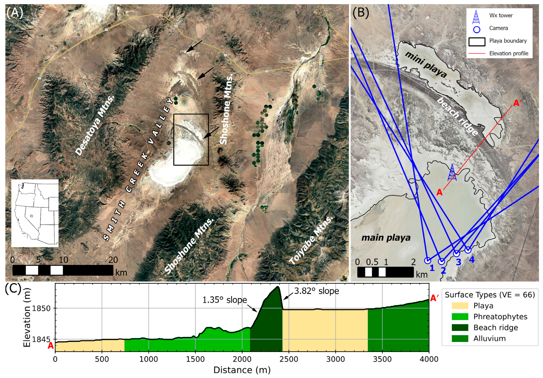
The analysis presented in this work uses data collected during a field campaign conducted in Smith Creek Valley (SCV), Nevada, USA, from 8 to 20 June 2019 and from 7 to 21 June 2021 [43]. Figure 1A shows the location of SCV, one of many similarly sized valleys situated within the Great Basin Desert. With a broad valley floor lying at an elevation of 1844 ± 2 m, SCV is surrounded by fault-block mountain ranges that rise 120–1300 m above the valley. These mountains primarily comprise Tertiary silicic ash-flow tuffs that are common in Nevada [45], with the valley’s basin fill consisting mainly of material eroded from these mountains [46].

A playa with a hard, compact silt and clay surface (here called the ‘main playa’) lies in the center of the valley, extending 11 km NE-SW and ~5 km NW-SE. In the study area, the main playa sits at an elevation of ~1845 m. A smaller playa (here called the ‘mini playa’) lies north of the main playa at an elevation of 1850 m, extending 1 km NE-SW and 5 km NW-SE. Numerous shoreline deposits ring the valley (some are pointed out in Figure 1A), indicating that a pluvial lake formed during the Pleistocene Epoch (‘Lake Desatoya’), with a depth reaching up to 57 m at an elevation of 1899 m [48]. One prominent 350 m wide, 3–7 m high beach ridge complex separates the main playa from the mini playa (Figure 1B).

An elevation profile (Figure 1C) illustrates the topographic relationships between the surfaces in which DDs were observed. From south to north along the profile A-A′, these areas included the bare (vegetation-free) surface of the main playa, a zone of hummocky ground alternating between low-lying valleys with sparsely vegetated playa-like surfaces and 2–4 m high hills covered by phreatophytic shrubs (mostly greasewood, Sarcobatus vermiculatus), the beach ridge complex rising 9 m above the main playa floor, the bare flat surface of the mini playa sitting 4 m below the beach ridge, and an alluvial plain vegetated with Sarcobatus vermiculatus rising steadily toward the Shoshone Mountains.

2.2. Experimental Setup

A description and the configuration of the 2019 field instruments are detailed in [43], with relevant portions briefly described here. Combining the methods of [49,50], we collected continuous meteorologic data and daytime images from 7 to 21 June 2019, with camera imaging constrained only by severe weather and occasional power limitations. We selected 11 June 2019 for detailed analysis in part because, after onset, DDs were plentiful and formed continuously throughout the day [43], and in part because the sky was cloud-free and thus did not interfere with automated DD detection. All four cameras began operating simultaneously at 9:09:54 local time (where ‘local time’ refers to Pacific Daylight Time, UTC-7). All successive references to time are in this local time.

2.2.1. Meteorology Instruments

A Campbell 10 m weather tower continuously monitored meteorological conditions throughout the field campaign, collecting a full set of data every 2 s. The tower was placed 50 m from the northeast margin of the main playa (Figure 1B), with the location selected to capture differences in conditions based on wind direction, regardless of where DDs were observed to form. Winds ranging from north-northwesterly to easterly represent flow across the hummocky, shrub-covered terrain north of the main playa, whereas winds from the remaining sector represent flow across kilometers of a flat, smooth playa surface. If these factors affect DD characteristics, then meteorological measurements representing conditions within these sectors may help determine when and how this happens (e.g., [51] found that DD production was suppressed where eddy heat fluxes were increased by high aerodynamic surface roughness).

The weather tower monitored the energy budget using a CS655 water content reflectometer, a Huskeflux soil heat flux plate that was buried to a depth of 8 cm, a CMP3 pyranometer to measure incoming solar radiation (wavelength range 0.3–2.8 μm), and an Apogee Infrared radiometer to measure emitted longwave radiation from the surface (wavelength range 8–14 μm). Using this data, [43] estimated that the playa surface albedo in 2019 was ~0.41 when not darkened by rain, and that the playa’s thermal inertia was relatively high with an upper limit value of ~1100 J m⁻² K⁻¹ s^½.

Anemometers (R.M. Young Wind Sentry model 03101) and thermistors (model 109) were placed on booms at different heights on the tower at approximately linear distances in log space. These instruments enabled wind and temperature profiling, leading to estimates of aerodynamic surface roughness. Reference [43] found these values to vary considerably with wind direction. Extraordinarily small surface roughness values of ~0.002 mm corresponded to winds crossing 10 km of flat smooth playa, whereas values up to ~8.5 mm corresponded to winds that had just blown over nearby hummocky, shrubby terrain.

A three-dimensional sonic anemometer (CSAT3B) and fine-wire thermocouple (model FW05) measured turbulent heat and momentum fluxes at a frequency of 20 Hz. These instruments were placed at a height of 5 m, 1.5–2 times the height of the phreatophyte canopy, to avoid the roughness sublayer produced by the shrubs and hummocks. A Vaisala barometer (model PTB110) and temperature/relative humidity probe (model HMP60) were located at the same height on the tower, but at a distance from the high frequency instruments to prevent contaminating their data.

2.2.2. Time-Lapse Stereo Imaging

We placed four Canon EOS 7D Mark II digital single-lens cameras (DSLR) (purchased from B&H Photo Video, New York City, NY, USA) on the eastern margin of the main playa, with fields of view (FOV) approximately centered on the weather tower (Figure 1B, [43]). The cameras were spaced ~500 m apart and set to a wide FOV (64.8°, f = 28.4 mm). This setup produced views that overlapped by 8–35° of arc at the center of each camera’s FOV, providing stereo coverage of the northern main playa. Each 20-megapixel image (5472 × 3648 pixels) was stored in Canon Raw Version 2 (‘CR2’) format. The cameras were set to autonomously and synchronously capture an image every 20 s.

2.3. Meteorological Conditions on 11 June 2019

The following summarizes meteorological conditions measured on 11 June 2019 by [43]. On the morning of 11 June 2019, the sky became cloudless at 8:00 and remained so throughout the rest of the day. After sunrise, at 5:23, ground temperatures rose from a minimum of 2.9 °C at 5:42 to a maximum of 36.2 °C at 13:40, and 10 m air temperatures rose from a minimum of 4.7 °C at 5:37 to a maximum of 28.3 °C at 15:58. Despite both air and ground temperature increases during the morning, ground temperatures did not exceed air temperatures until ~9:45, almost 4.5 h after sunrise.

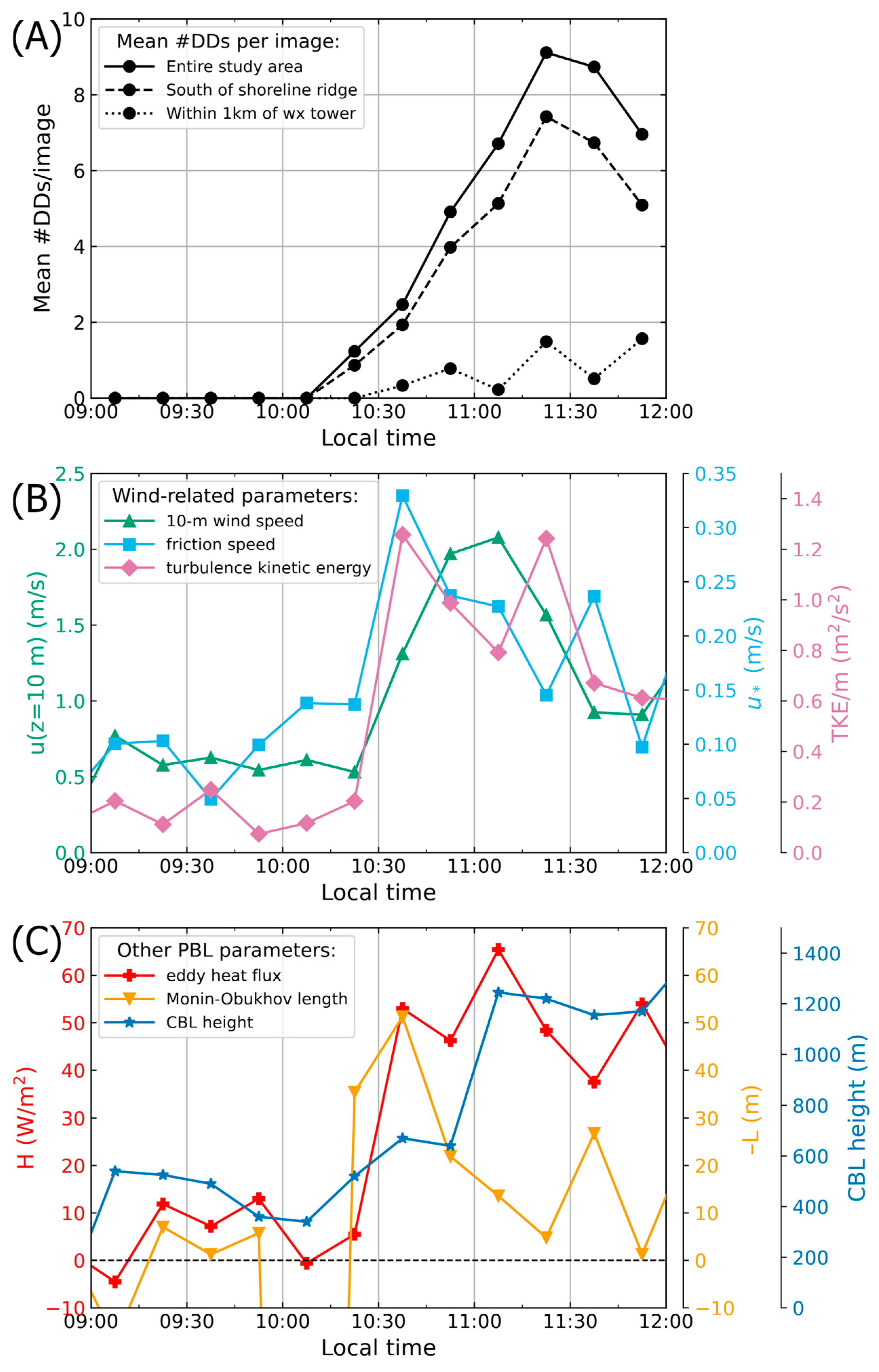
Several factors indicated that convective activity abruptly escalated between 10:15 and 10:45. First, the water vapor mixing ratio remained at ~5 g/kg until ~10:20, when it abruptly dropped to ~3 g/kg over the following 40 min. This sudden drop in moisture coincided with the onset of DD production (Section 4.1), suggesting that dry air was mixed from aloft as convective activity strengthened. Second, 15 min averaged wind speeds increased. From 9:00 to 10:30, winds were light at ~1 m/s (SW), with gusts <2 m/s. Beginning at 10:30, winds increased only slightly to 1.5–2 m/s (NW to E), but gust speeds increased considerably to 2.5–5 m/s. Third, at 10:30, eddy fluxes reflected this sudden increase in gustiness, with the heat flux increasing from ~5 to ~50 W/m² and the friction speed ($u_{\ast }$) more than doubling from ~0.1 m/s to >0.2 m/s. Over the same time period, the turbulence kinetic energy (TKE/m) increased from 0.2 to 1.3 m²/s².

The rapid mid-morning shift in playa conditions was attributed to the presence of a strongly stable boundary layer at night, as the high albedo and high thermal inertia of the playa would both delay local surface heating [43]. Further, possible (although unmeasured) latent heat flux from snowmelt ponded elsewhere on the playa may have additionally inhibited the growth of sensible heat flux. Strongly stratified near-surface air can suppress growth of the convective boundary layer until thermals are able to ‘punch’ through this stable layer, leading to a sudden onset of convective turnover (e.g., [52]).

3. Analysis Methods

We analyzed images beginning after all four cameras were turned on (at 9:09:54). Our analysis was conducted on each set of images obtained until noon (11:59:54), for a total of 511 ‘timesteps’.

3.1. Stereogrammetric Triangulation

3.1.1. DD Identification

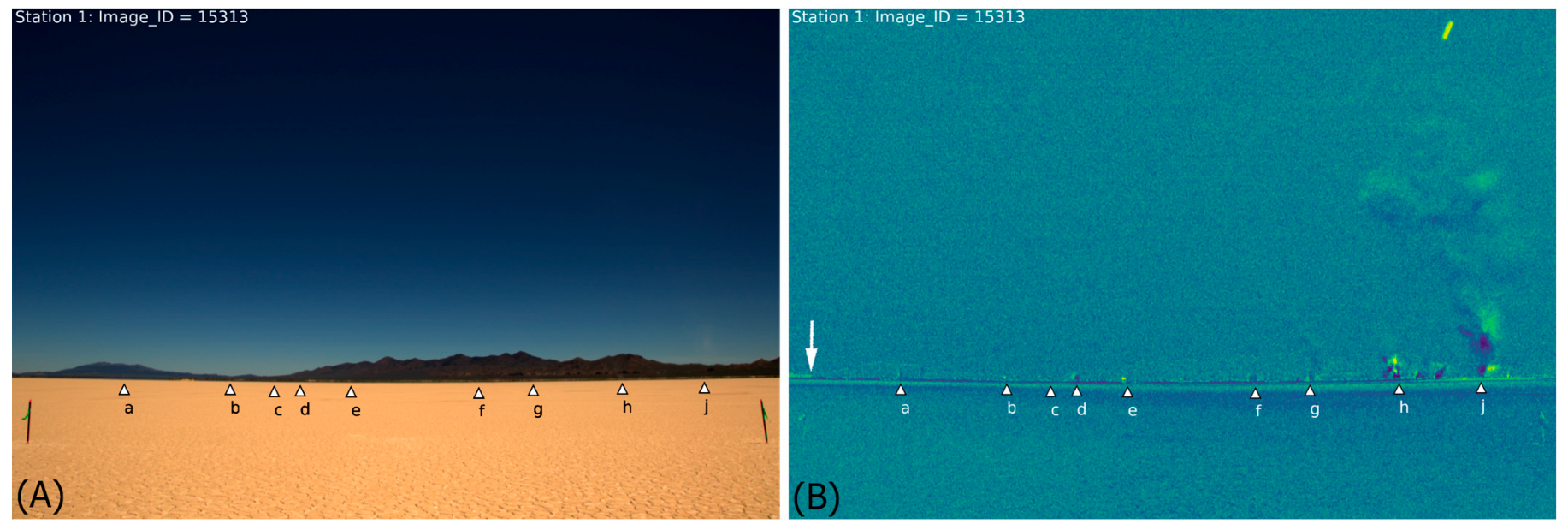
The first step in triangulating DDs was to identify them in images, and then record their horizontal (U) and vertical (V) image pixel coordinates in each camera frame and for each timestep (i.e., each camera frame, e.g., Figure S1). We wrote Python (version 3.13) code to display time-differenced frames for each camera (e.g., Figure S2). Using a graphical user interface (GUI), the apparent base of each DD in each camera frame was selected manually (by LKF) and its image pixel coordinates were automatically recorded to a table (see Supplementary Materials). Each identified DD was assigned a lowercase identifying letter, such that each image timestamp and assigned letter corresponded to a single occurrence of a DD. Here we refer to each occurrence as a ‘DD instance’. Figure 2A shows an example of an image timestep from one of the four cameras, containing 9 DD instances (identifiers ‘a’ through ‘j’). Even though the image contrast has been enhanced for publication, most of the DDs in the distance are difficult to spot. As previously found [49], DDs become much more apparent when differencing sequential timesteps, as shown in Figure 2B. For example, DD instance ‘j’ is the most prominent, with a tall plume. In differenced images, the leading edge of the DD becomes brighter (yellow) due to the dust load reflecting more sunlight than the previous frame. The trailing edge of the DD is darker relative to the previous frame (purple). Therefore, the purple-to-yellow color contrast indicates that DD instance ‘j’ is translating from left to right.

Nearly all visible DDs were labeled in Figure 2, with some caveats. Although the FOVs of the four cameras largely overlapped, there were ‘blind spots’ where DDs might be visible in fewer images. To triangulate their locations, DDs had to be identified in at least two camera frames from the same timestep. Where they were not visible in at least two frames, they were not marked. DDs also needed to be visually distinct to be confidently labeled and correlated in each of the cameras. For example, there are two small dust plumes between DDs ‘h’ and ‘j’ in Figure 2, which are unlabeled because they were not confidently identified in the other camera frames of this timestep. Another nuance of labeling DDs occurred when an optically thick DD passed in front of a smaller or fainter one, which typically occurred in one or two, but not all camera FOVs of that timestep. To track the quality of each DD instance, an index from 1 to 3 was assigned based on our confidence in the DD’s identification and correlation among cameras (e.g., a value of ‘1’ indicated a DD of some opacity and size, with a shape distinctive enough to permit a high level of confidence, whereas a value of ‘3’ corresponded to DDs that were faint, with correlations inferred from positions in previous timesteps).

A rough estimate of human error in determining DD position can be made by comparing the manually determined horizontal pixel coordinates (U) with automatically determined locations used to calculate DD widths, the latter of which was conducted for a limited set of DD instances in Camera Station #4 (described in Section 3.2.2). The median difference between the manual and automated U coordinate was 6 pixels. By doubling this value to 12 pixels, we approximate the compounded uncertainty in manually determined DD positions from multiple cameras, as well as the uncertainty inherent in faint, very wide, or complexly shaped DDs (i.e., those not included in width determinations). At a distance of 1 km, this horizontal uncertainty is ±3 m, and at 5 km it is ±14 m, i.e., the approximate location uncertainty from manual horizontal coordinate selection is of the order of one or two DD diameters. We also note that DDs located beyond the beach ridge may have additional position uncertainty, as the beach ridge would have blocked views of the DD bases.

3.1.2. DD Localization

The roughly linear, widely spaced configuration of ground-based digital cameras (Figure 1B) provided sufficient parallax to enable the localization of DDs using structure-from-motion and multi-view geometry methods. Agisoft Metashape Professional (version 2.2.0 build 19890, 64 bit) was used to perform camera calibration, image alignment, and 3D reconstruction, enabling estimation of camera parameters and triangulation of point locations from overlapping image frames.

Camera stations were initially surveyed using a handheld Garmin global navigation satellite system (GNSS, manufactured by DeLorme in Yarmouth, Maine, USA), providing only meter-scale position accuracy in the local geographic frame. The project’s geographical reference frame was refined using a subset of images from four cameras, imported and automatically aligned in a Metashape project. Stable landmarks (e.g., mountain peaks, vegetation patterns, rock outcrops, and human-made features) were identified within the image frames and used as tie points. These landmarks were identified in georeferenced satellite and aerial imagery, and their geographic coordinates were extracted and imported into Metashape as ground control points (GCPs). Their corresponding image projections (U,V) were manually identified in each camera view. Metashape’s camera optimization (bundle adjustment) simultaneously refined interior orientation parameters, estimated camera poses, and aligned the solution to a WGS84 datum, projected into UTM Zone 11N.

Because the landmarks span large distances relative to the camera spacing, the resulting geometry provided strong constraints on camera position and orientation, ensuring that all reconstructed DD positions were expressed in physically meaningful ground coordinates. Reprojection residuals for the optimized cameras were low (sub-pixel;

Table 1. Camera positions, orientations, and associated uncertainties from the bundle adjustment. Positional and angular errors represent estimated uncertainties in camera location and orientation, respectively. The number of projections indicates the total contributing image observations, and pixel error corresponds to the mean reprojection residual. Coordinates are reported in UTM Zone 10N with applied offsets (Easting: +459 km, Northing: +4352 km, Elevation: +1.8 km).

Cam	X (m)	Y (m)	Z (m)	Error (m)	Yaw (°)	Pitch (°)	Roll (°)	Error (°)	Projections	Error (Pix)
1	182	122	0.3	0.06	23.7 NE	−9.9	−1.5	1.4	168	0.59
2	692	84	0.3	0.19	9.7 NE	−12.0	0.9	1.4	228	0.78
3	232	365	0.3	0.24	7.5 NE	−14.8	−0.8	1.2	219	0.81
4	671	494	0.2	0.09	0 N	−10.7	−0.7	1.4	150	0.55
Total Error:				0.16				1.4

), indicating a stable and internally consistent solution.

Ground control points used to constrain the solution were located several kilometers from the camera array (

Table 2. Ground control point (GCP) coordinates used to constrain the bundle adjustment, reported in UTM Zone 10N with applied offsets (Easting: +459 km, Northing: +4352 km, Elevation: +1.8 km). The number of projections indicates that each GCP was observed in all four images. Pixel error (Error (pix)) represents the reprojection residual, while object-space error (Error (m)) reflects the residual of each point after adjustment. The larger object-space errors relative to pixel residuals are consistent with long-range intersection geometry, where small angular uncertainties propagate to meter-scale positional errors.

GCP	X (m)	Y (m)	Z (m)	Error (m)	Projections	Error (Pix)
1	4796	5382	108	4.5	4	0.88
2	4701	6105	120	2.8	4	0.70
3	4498	7716	122	9.5	4	0.79
4	6104	10,378	356	13.0	4	1.39
5	4078	15,506	173	11.1	4	2.77
6	5979	11,853	519	1.2	4	0.97
7	5363	16,561	410	6.1	4	2.00
8	1388	33,115	571	3.8	4	2.75

). These GCPs, which include mountain peaks and other stable features visible in all four cameras, were located approximately 5.6–17 km from the cameras and exhibited reprojection errors of ~0.70–2.77 pixels, corresponding to object-space residuals of ~1.2–13.0 m. These values were consistent with expected geometric error propagation under long-range viewing conditions, where small image-space uncertainties produced meter-scale positional errors when projected over kilometer-scale distances. As such, these residuals represent an upper bound on positional uncertainty imposed by viewing geometry rather than a limitation of image measurement precision.

In contrast, scale constraints defined within the near field of view provided a more representative estimate of expected accuracy for DD localization. Known distances (~15.3–15.7 m) measured between field markers show absolute errors of −0.35 to +0.14 m, reflecting substantially reduced propagation of image-space uncertainty under short-baseline conditions. Because positional uncertainty scales approximately with distance for a given level of image-space error, these results indicated that features located within the camera FOVs—such as the DDs analyzed here—were resolved under favorable geometric conditions for triangulation. The mean angular uncertainty across all GCP’s individual reprojection errors is 0.020°.

DDs observed simultaneously from multiple viewpoints were treated as pseudo-GCPs with unknown object-space coordinates. Using the calibrated and georeferenced camera models, Metashape solved for the 3D position of each DD instance by minimizing the reprojection error between observed pixel locations and the projections of the reconstructed point into each camera’s view. Each observation defines a line of sight from the camera center into the scene, and the DD position corresponds to the point of best intersection of these rays. Observations from three or four cameras provided overdetermined solutions, while two-camera observations represented simpler intersections that were more sensitive to viewing geometry.

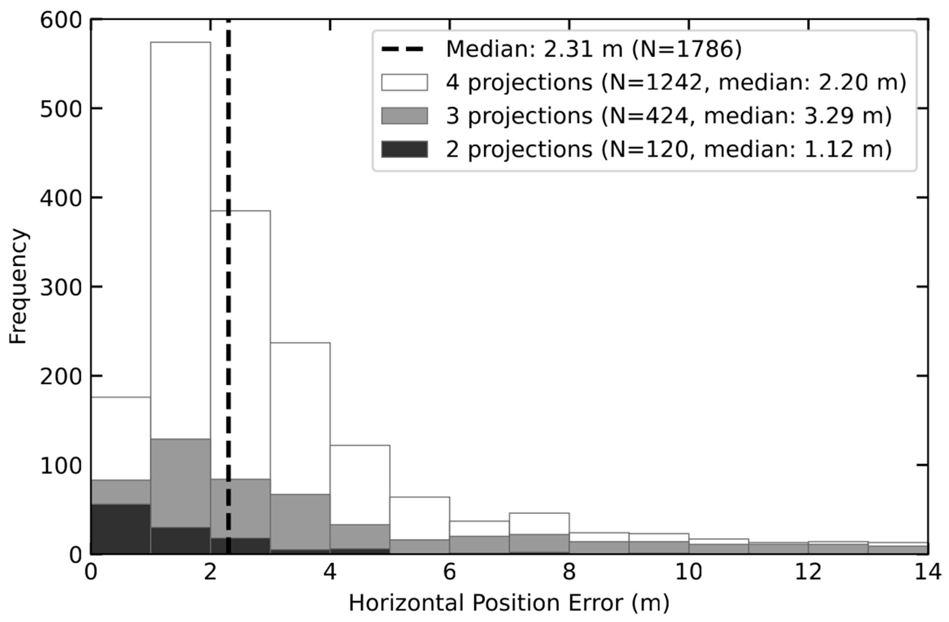
Uncertainty in DD positions was estimated from image-space residuals scaled by viewing geometry, with horizontal positional uncertainty (σ_xy) providing the most robust measure of localization accuracy (

Table 3. Summary statistics of horizontal positional uncertainty (σ_xy) for DD locations derived from multi-view image intersections, scaled by $1/\sqrt{N_c}$ to adjust for projection count.

DD instance count (N)	1786
Mean (m)	3.55
Standard Deviation (m)	5.02
Minimum (m)	0.01
Q1, 25% (m)	1.45
Q2/median, 50% (m)	2.31
Q3, 75% (m)	3.82
P95 (m)	10.4
Maximum (m)	128.57
2 projection, mean ± std (m)	1.81 ± 3.76
3 projection, mean ± std (m)	5.14 ± 5.38
4 projection, mean ± std (m)	3.18 ± 4.88

; Figure 3). This approach provided a practical estimate of positional uncertainty based on image-space residuals and viewing geometry, rather than a full covariance propagation from the bundle adjustment. For each point, the reprojection error was converted to an angular uncertainty by dividing by the focal length (in pixels) and projected into ground coordinates using the mean horizontal distance to the observing cameras. To account for weaker geometric constraints in cases with fewer projections (e.g., two cameras provide only one ray intersection), the results were scaled by $1/\sqrt{N_c}$, where $N_c$ is the number of cameras that observed the DD. This follows standard error propagation for independent observations and provides a first-order approximation of positional uncertainty, though it does not capture the full covariance structure of the multi-ray intersection. The analysis focused on horizontal positional uncertainty, as vertical estimates were more sensitive to viewing geometry and less reliable for these observations. The distribution of σ_xy was strongly right-skewed, with an overall median of 2.31 m (N = 1786) and an interquartile range of 1.45–3.82 m, indicating that most solutions were concentrated within the low meter-scale range. Although the mean uncertainty (3.55 m) was elevated by a small number of large-uncertainty cases, these outliers do not reflect typical performance; the majority of DD positions were resolved with horizontal uncertainties on the order of a few meters. The 95th percentile error provides an upper bound on typical performance and is approximately 10.4 m.

Projection-dependent ($N_c$) statistics are included for reference, reported as mean ± std (σ_xy), and indicate that geometric redundancy contributes to solution stability. Four-projection solutions (N = 1242) exhibit a mean uncertainty of 3.18 ± 4.88 m, while three-projection solutions (N = 424) show a broader distribution and higher mean uncertainty (5.14 ± 5.38 m). Two-projection solutions (N = 120) exhibit a lowest mean uncertainty (1.81 ± 3.76 m) but represent a limited subset characterized by underdetermined estimates of uncertainty due to only a single ray intersection and therefore do not reflect a clear framing of geometric accuracy. However, we note that all observations have uncertainty estimates that are sub-decimeter and improve from 3 to 4 observing cameras. Median and interquartile statistics provide the most representative measures of typical localization uncertainty. The histogram in Figure 3 illustrates the concentration of low-uncertainty solutions and a small population of higher-uncertainty cases defining the upper tail of the distribution. As a demonstration, image projections were obtained of a car crossing the camera FOVs along the beach ridge gravel road, providing an example of four-projection solutions that placed the car on or very close to the road (Figure S3).

Following triangulation, DD coordinates were exported from Metashape in the same geographic reference frame used for the camera and GCP data. For each instance, the reprojection residual between measured and predicted pixel locations provides a direct indicator of localization quality. Instances with large residuals—typically corresponding to faint, partially obscured, or poorly constrained observations—were identified using consistent reprojection residual thresholds and excluded from further analysis. Because the camera array provides substantial parallax over ~500 m spacing, the majority of DD reconstructions were well conditioned and yielded consistent, meter-scale horizontal accuracy suitable for subsequent spatial analysis.

3.2. Data Analysis

We constructed a spreadsheet (see Supplementary Materials) containing one row for each DD instance, adding new fields as calculations were made. Prior to the analysis, the fields included the datetime (image timestamp), a lowercase letter identifier (e.g., Figure 2), an identification confidence index, the number of camera images ($N_c)$ in which each DD instance was identified (2, 3, or 4), the U and V pixel positions of the DD in each camera, and the corresponding projected X and Y locations in UTM Zone 11N coordinates. Maps throughout were created using ArcGIS^® Desktop (version 10.5) by Esri.

3.2.1. Identifying Sequences of DDs

Sequences of DDs were manually identified by comparing the shapes and positions of DD instances from one timestep to another. DDs tended to translate at a constant direction and speed, and their shapes and brightnesses did not often vary substantially over the 20 s sampling period. As a result, it is generally possible to recognize the same DD in different cameras or subsequent timesteps based on its expected location and physical characteristics. This fact enabled analysis of initiation locations and DD evolution.

3.2.2. Measuring DD Widths, Relative Dustiness, and Shape

Given a known location and distance from a camera, the width of a DD may be determined by the number of pixels it spans horizontally across an image. This pixel width ($w_p$) may be converted to width in meters ($w_m$) by calculating the arc length of these pixels, i.e., ${w_m=w}_{p}d$ (pixel pitch/focal length), where $d$ is the distance from the camera to the DD, and the pixel pitch and focal length of the DSLRs are 4.17 μm and 18 mm, respectively. We measured DD widths using Camera Station #4 because it was closest to, and thus best resolved, the observed DDs. Once the widths were determined, the mean uncalibrated brightness (i.e., digital number, or DN) in a 3-pixel high region along the DD’s width serves as a proxy for relative dust opacity.

Therein ends the straightforward part of measuring DD widths, because selecting a method to consistently and objectively measure apparent $w_p$ is fraught with complications—even at our field site, with its relatively simple geometry. First, DDs may vary in width along their height, depending on turbulent diffusion that affects both dust lifting and transport on subsecond timescales. To estimate vertical dust fluxes at the surface, DD widths would ideally be measured just above the surface. However, DD bases were not always visible from the vantage point of the cameras, such as when (1) one DD crossed in front of another, (2) a DD was located beyond the margin of the bare playa and the base was obscured by shrubs and hummocks, and/or (3) the base of a DD was obscured by an inferior mirage (i.e., turbulent air refracts light, causing the image to be mirrored below the actual object). Second, the width must be measured against a constant background to ensure that both the width and relative brightness measurements are consistent as the DD moves from one location to another. Third, the sharpness of the outside ‘edge’ of a DD varied with the amount and distribution of dust, potentially making manual width determination subjective and limiting automated width determination to the most ideal cases. For example, opaque DDs often had distinct margins, whereas relatively dust-poor DDs generally have more diffuse margins. Suitable criteria are required to ensure unbiased and consistent measurements.

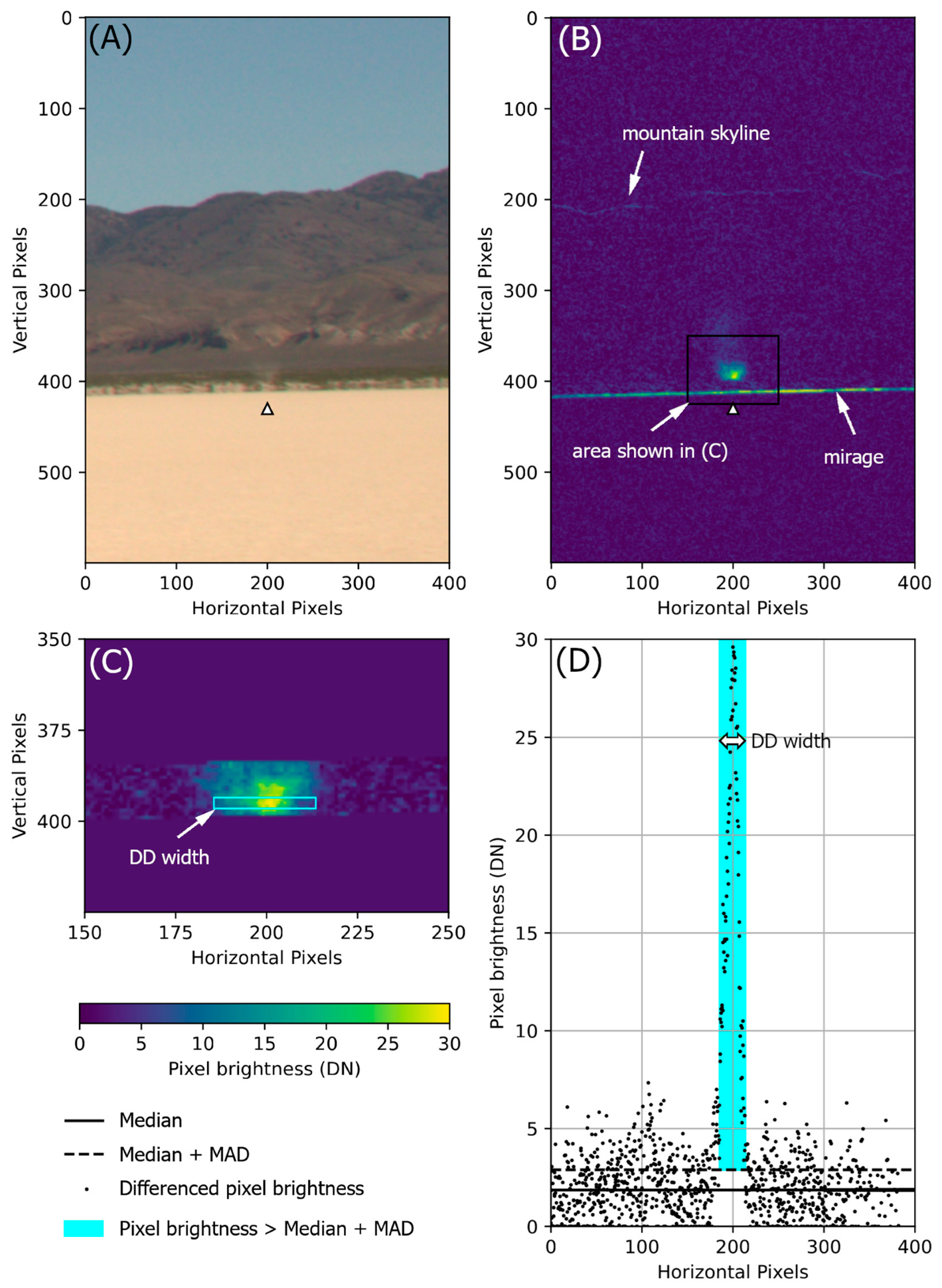
To address the above potential pitfalls, we created a semi-automated method to measure DD widths (see the example in Figure 4). First, each DD instance was isolated in a 400 pixel-wide × 600 pixel-high image area centered on the instance (Figure 4A). The color images were converted from RGB encodings to equivalent grayscale using the following commonly applied weighted mean brightness: 0.299R + 0.587G + 0.114B. We then isolated the lofted dust by subtracting from each image the darkest (i.e., dust-free) pixels in the surrounding six image timesteps (three before and three after). Each resulting difference image contained only time-varying features and noise (Figure 4B). Other than the lofted dust of each DD in the image, these temporally changing features commonly included a mirage that refracted the view from a horizontal line along the playa surface, and occasionally, from among the visible vegetation-free hummocky regions. Similarly, in some cases, wind gusts would move the camera enough to create an enhanced skyline along the background mountaintops.

We then applied a mask to each difference image that limited automated DD measurement to a 15-pixel high region just above the hummocky region, which both ensured a relatively uniform background against the far alluvial plain and excluded the mirage layer and mountain skyline (Figure 4C and Figure S4). A 2D Gaussian blur of 5 × 5 pixels was applied to the difference image to locate the brightest point in the DD, which was assumed to be representative of the most opaque part of the dust-lofting vortex. From this brightest point, each adjacent pixel to the left and right of the original difference image was considered to be part of the DD’s width if its brightness exceeded a statistically significant background noise level along a 400 pixel-wide × 3 pixel-high area centered on the DD. This upper limit to the background noise was defined by the median brightness plus the median absolute deviation (MAD) brightness, providing a robust measure of the high end of background brightness dispersion (i.e., this value is not sensitive to pixel brightnesses within the DD). Figure 4D shows an example of pixel brightnesses from the 400 × 3 pixel area centered on a DD, in which brightnesses within the cyan area were considered to be part of the DD (the same pixels are also outlined in Figure 4C). The width of the cyan area represents the DD width, and the mean brightness within the cyan area is a measure of the DD’s relative dust content. We note that using the mean brightness to infer relative dust content neglects factors such as particle size distribution, which may vary spatially from the phreatophytic hummocky region to the bare playa, as well as internal shading from 0.1–2 m scale dusty structures within the dust devil.

The above automated method produced several false or incomplete detections, requiring evaluation and, where possible, correction. Each DD instance measurement was manually inspected and assigned a quality value to the column ‘W_quality’ (see Supplementary Materials) according to the success of the measurement. DDs with widths that were correctly determined were given a ‘W_quality’ value of ‘1’ (e.g., Figure 4). Values of ‘0’ generally corresponded to very faint DDs in which pixel DNs did not rise sufficiently above the background noise (median + MAD) to provide a width measurement. Widths less than 3 pixels were included in this category. In some cases, one DD would pass close to another, such that the width measurement erroneously included either both DDs or the wrong (brighter) DD. In cases where these overlapping signals could not be separated (e.g., Figure S5), the ‘W_quality’ was assigned a value of ‘0OLXX’ (with the ‘OL’ indicating an overlap issue and ‘XX’ corresponding to the sequence ID of the overlapping DD). Some overlap cases were corrected by masking out DDs that were not the intended target (e.g., Figure S6) and were assigned a ‘W_quality’ value of ‘1OLXX’. For DDs with diffuse and complex structures, the algorithm often identified a portion of the DD’s width (‘incomplete’, Figure S7). These widths were assigned a ‘W_quality’ of ‘2’ and should be regarded as lower limit widths. Of the measured DD instances, 63.1% had quality values of ‘1’, and 2.8% had ‘1OL’ for a total of 66.0% successful width measurements; 18.3% had quality values of ‘0’, and 5.3% had ‘0OL’ for a total of 23.6% unsuccessful width measurements; and 10.6% had quality values of ‘2’, indicating incomplete width measurements. In the following analysis, we included only successful width measurements.

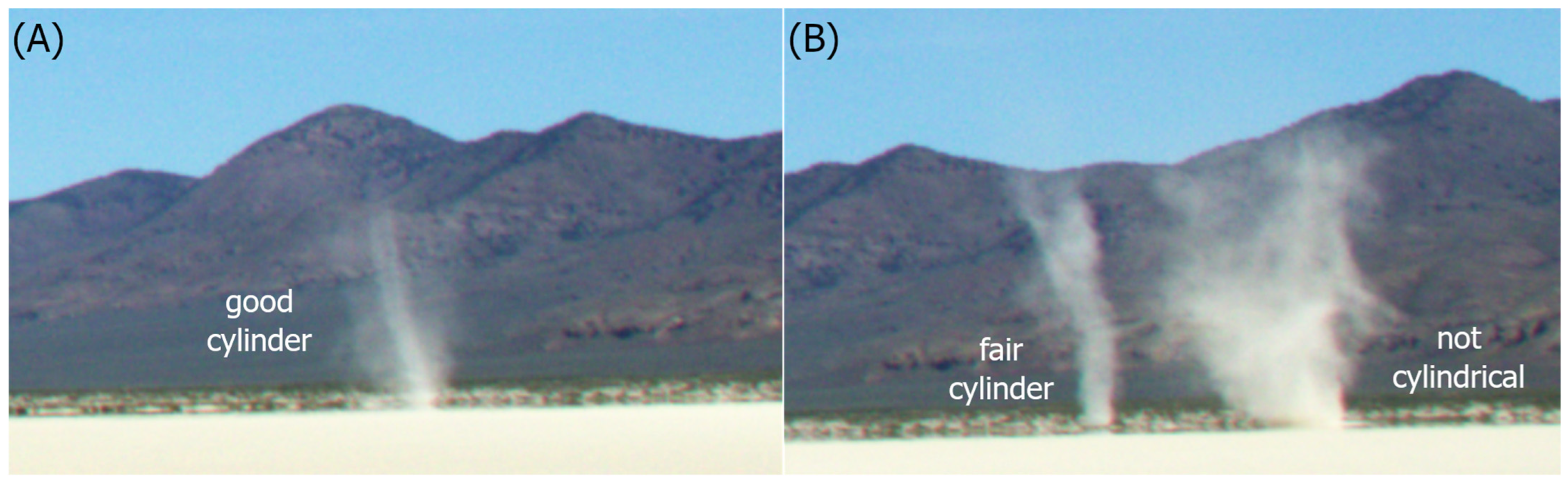
While manually evaluating width measurements, the qualitative closeness to a cylindrical shape was also noted. This aspect was tracked in part because [43] found DD shape to vary with wind speed, but also because these shapes are relatively rare and other factors may be required to produce a tight cylindrical shape. Further, we sought to investigate whether the morphology and structure of DDs relate to their longevity or size (i.e., their dust-lofting capacity). DDs with sharp-edged and cylindrical-shaped dust walls were given a ‘Cylindrical’ value of ‘1’ (i.e., ‘good cylindrical’, Figure 5A). DDs with a somewhat cylindrical shape, but with more diffuse or irregular edges, were assigned a value of ‘2’ (i.e., ‘fair cylindrical’); and those not exhibiting a cylindrical shape were assigned a value of ‘0’ (Figure 5B).

4. Results

4.1. The DD Database

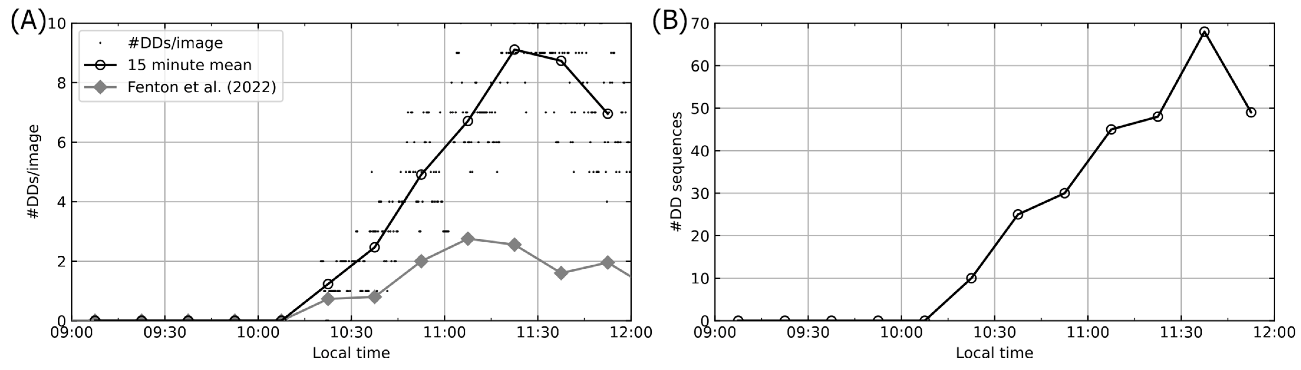
We identified a total of 1786 DD instances that passed through at least two camera FOVs on the morning of 11 June 2019, from 9:09:54 through 11:59:54 local time. These instances consist of 245 individual DDs, comprising 220 multiple-instance sequences (i.e., DDs that were seen on at least two successive timesteps) and 25 solo instances (i.e., DDs that were only identified in one timestep). Figure 6 shows the mean number of DDs and DD sequences, per image timestep, observed throughout the measured period.

The first DD of the morning appeared at 10:20:14, on the alluvial plain north of the playas. Once DD activity began, there were only four timesteps in which DDs were not observed, each of which occurred early in the study period (10:21:54, 10:22:14, 10:22:34, and 10:29:54). After the onset of activity, the number of DDs observed per image increased linearly until 11:30 and then dropped slightly from 11:30 to 12:00 (Figure 6A). Similarly, the number of DD sequences active in 15 min periods increased linearly until 11:45 and then dropped from 11:45 to 12:00 (Figure 6B). Figure 6A also shows the 15 min mean count of DDs presented by [43] using Camera Station #1 over the same time period. Because that study did not use time-differenced images, many fainter DDs were not counted, and thus this previous count is most representative of the largest and most optically thick DDs.

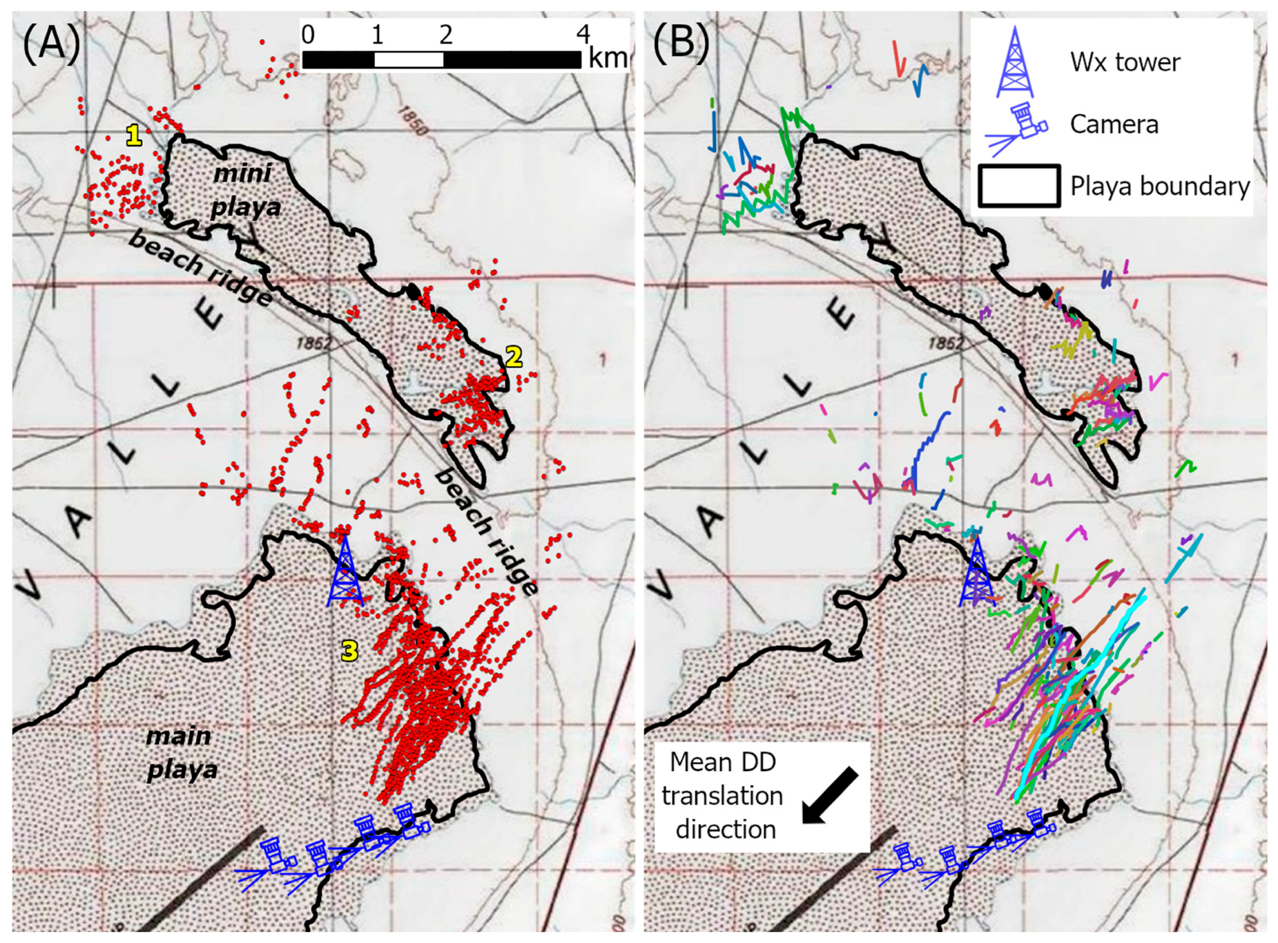
Figure 7 shows that the spatial distribution of DD observations was not uniform. The view in Figure 7 is zoomed in to highlight the majority of the DD occurrences; full maps of the entire dataset are shown in Figure S8. Most DD instances were located on bare playa surfaces, with 900 (50%) found on the main playa, 199 (11%) found on the mini playa, and 687 (38%) found on the surrounding vegetated areas. DDs concentrated in three regions: west of the mini playa, in the eastern region of the mini playa, and in the northeastern region of the main playa (labeled as ‘1’, ‘2’, and ‘3’ in Figure 7A, respectively). In this data set, no DDs that fully dissipated appear to have reformed again downwind. In addition, only one DD sequence appears to have crossed the beach ridge (Sequence #130, in area ‘1’). However, each of the Sequence #130 instances was poorly localized, with horizontal position errors >10 m, so it is possible that this DD did not cross the beach ridge.

4.2. DDs South of the Beach Ridge

For two reasons, we conducted the remainder of the data analysis only on DD instances and sequences found south of the beach ridge. First, these DDs represented a single micro-climate region of Smith Creek Valley, in that they occurred on or near the main playa. As a result, any temporal and spatial variations in DD behavior may be interpreted in the context of this environment, whereas DDs located elsewhere may have been influenced by different local conditions. Second, the meteorological tower was located in their midst, recording local conditions most representative of the region in which these DDs formed, evolved, and dissipated. The subset of DDs south of the beach ridge complex consisted of 1387 instances (78% of all 1786 instances) comprising 159 sequences (72% of all 220 sequences) and 24 solo occurrences (the only other observed solo DD formed on the mini playa). The first DD south of the beach ridge occurred at 10:23:54, or 3.33 min after DD onset observed in the broader camera suite FOV.

South of the beach ridge, overlapping camera FOVs form an irregular polygon with area $A$ = 28.63 km² (Figure S9). Over the 1.6 h duration of DD activity from 10:23:54 to 11:59:54, the 183 observed DDs’ (sequences + solo occurrences) mean areal density was 4.0 km⁻² h⁻¹. Given that DD counts during previous surveys tended to follow an areal density rate of $~50/A$ per day [41,54], this relationship suggests a typical value for our site would be 1.7 km⁻² day⁻¹. The pulse of morning DD activity was the strongest during this day, but DDs continued to form until 18:03:33 [43], suggesting that the areal density south of the beach ridge was >6 km⁻² day⁻¹. This indicates that on 11 June 2019, the SCV study area exhibited a high rate of DD formation relative to most observational sites.

4.2.1. DD Duration and Formation Sites

The duration of each DD sequence was determined by the time of its first and last sighting. As a result, many durations are lower limits, as DDs within the camera FOVs may have formed up to 20 s before the first sighting and lasted up to 20 s after the last sighting. Further, some DDs likely lasted longer than observed because they either translated into the camera FOVs after forming, or out of the camera FOVs while still active (i.e., they ‘entered onstage’ and ‘exited offstage’). For example, the longest observed DD ran for 18.33 min, from 10:40:54 to 10:59:14, beginning just southwest of the beach ridge and translating SSW for 2.6 km onto the main playa (Sequence #32, highlighted in cyan in Figure 7B). In the first sighting of this DD, it appeared near the center of each camera frame, so that its initiation was fully captured in our images. However, the DD eventually traveled out of the overlapping camera FOVs, continuing further along the playa for an unrecorded duration, so it may have lasted much longer.

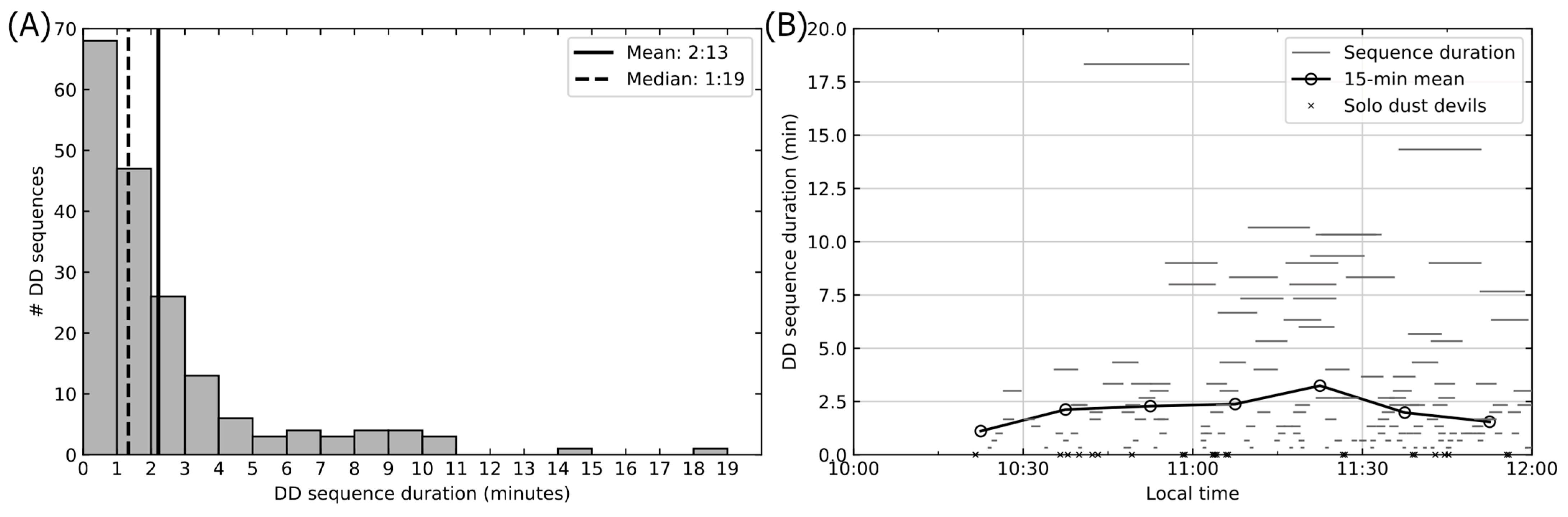
Figure 8A shows a histogram of DD sequence durations in 1 min bins. The modal duration lies at <1 min, and the mean duration of all 159 sequences and 24 solo instances is 2.22 min. Figure 8B shows a timeline of DD sequence duration. Solo DDs, shown as ‘×’-shaped points with a duration of 0 min, occurred throughout the observation period. The 15 min mean sequence duration is also shown in Figure 8B, increasing from ~1 min at DD onset to a steady duration of ~2.5 min, peaking at 3.25 min from 11:15 to 11:30, and then dropping to 1.5 min after 11:45. This peak occurs at the same time as the maximum 15 min mean number of DD instances per image (Figure 6A). This correlation suggests that the processes enhancing DD generation also increase their duration.

In any given region, DDs are known to preferentially form in some locations more than others, as they are influenced by spatial variations in surface roughness, heat flux, and sediment availability [51,55,56]. At our field site, DDs south of the beach ridge formed on and off the bare playa in nearly equal numbers (Figure S10), with 72 initial sightings on the main playa and 87 off the main playa (45% and 55%, respectively). Of these sequences, those that formed off the edge of the main playa tended to end before translating onto the main playa (63 sequences, or 72% of sequences that formed off the playa edge). These off-playa DDs were generally short-lived, with a mean duration of 1.48 min (Figure S11A), and occurred throughout the observation period (Figure S11B). Further, most of the solo sightings south of the beach ridge (18 of 24, or 75%) were located off the main playa. In contrast, those DDs that either initiated on or traversed onto the playa lasted longer than those that remained outside the main playa. Those that formed on the playa had a mean duration of 2.70 min, and those that formed off the playa but traversed onto the bare playa surface had a mean duration of 5.00 min. This pattern suggests that the bare playa surface created conditions that enhanced DD stability, relative to conditions off the playa.

4.2.2. DD Widths and Brightness

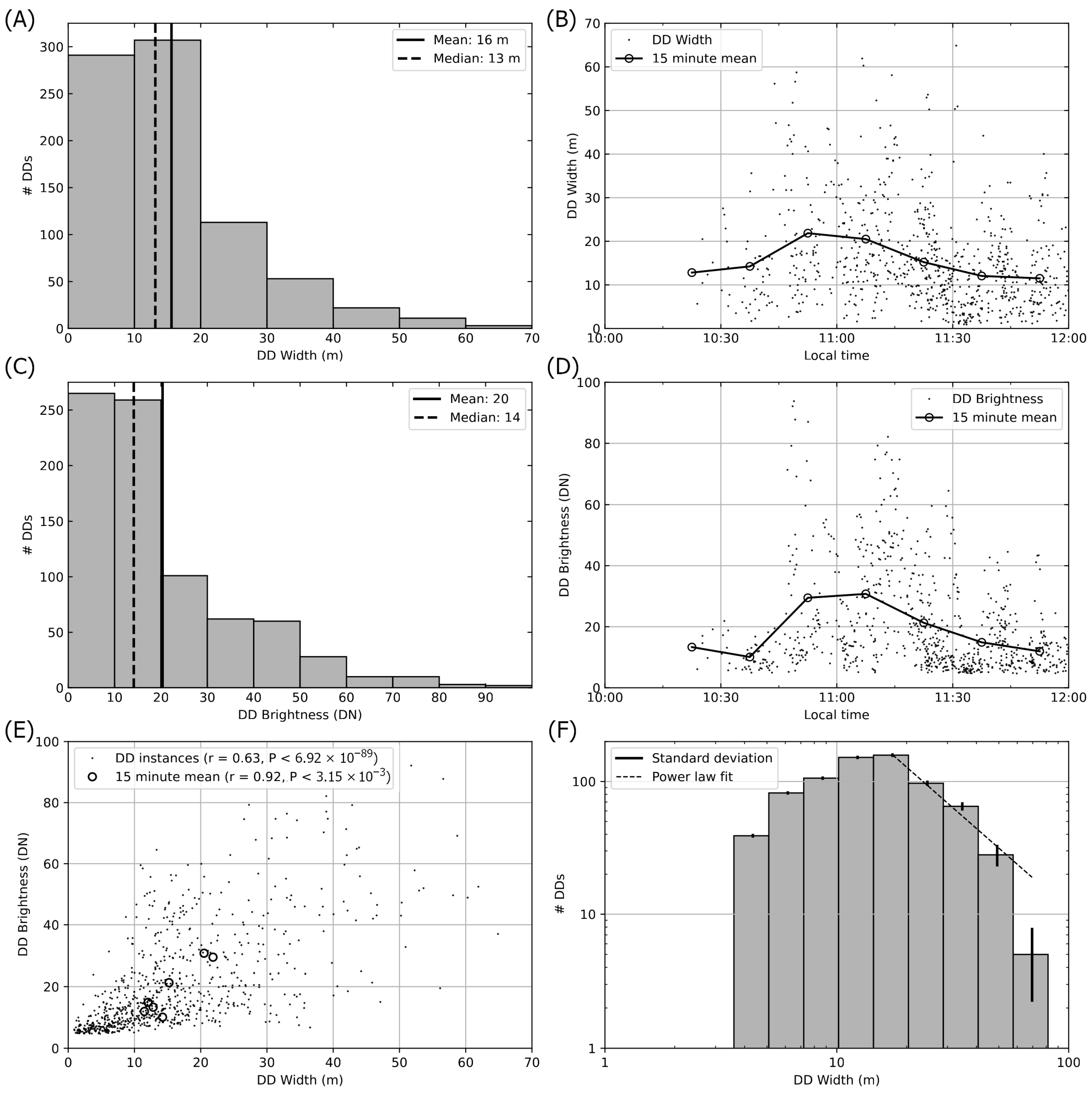
Of the 1387 DD instances identified south of the beach ridge, 800 widths and brightnesses were measured successfully. These measurements were drawn from 143 multiple-instance DD sequences and 13 solo DD instances. Figure 9A shows that the modal, mean, and median widths all fell between 10 and 20 m, similar to widths measured in previous DD field surveys on Earth [17,57,58]. Fifteen-minute mean DD widths measured over time (Figure 9B) varied between 11 and 22 m, with 15 min mean values peaking between 10:45 and 11:15. The histogram in Figure 9C shows that the majority of DDs were relatively diffuse (i.e., they had a low brightness value); the DD instance shown in Figure 4 is a typical example with a moderately sized width (16 m) that is fairly diffuse (brightness DN value of 17). Similar to the DD widths, 15 min mean brightnesses peaked between 10:45 and 11:15 (Figure 9D). When DD width and brightness are plotted together (Figure 9E), a moderate correlation emerges, reflecting longer dust-laden path lengths of wider DDs.

One application of our width dataset is a measure of DD width distribution, which is key for estimating and extrapolating dust fluxes (e.g., [59]). For comparison, we fit the number of DDs ($N$) of width ($w$) to a differential power law ($N\left(w\right)=a{w}^b$). To best determine this relationship, we first recognize that narrow DDs are more difficult to identify with increasing distance from the camera suite. From the DD population south of the beach ridge, the farthest DD instance was located 5.185 km from Camera Station #4. At this distance, the narrowest DD the camera could identify, assuming a minimum width spanning 3 pixels, would be 3.6 m wide. We thus bin the width data following [58], using differential width bins that increase in size with a ratio of $\sqrt{2}$ and begin with the narrowest reliable width measurement (i.e., bins are $3.6$ m, $3.6\sqrt{2}$ m, $3.6{\left(\sqrt{2}\right)}^2$ m, $3.6{\left(\sqrt{2}\right)}^3$ m, etc.). The resulting histogram plotted in (Figure 9F) consists of 732 measurements with widths >3.6 m. The distribution peaks in the 14.4–20.4 m bin, which is much larger than the estimated 3-pixel lower limit of 3.6 m. It is unclear whether this low-end ‘rolloff’ truly reflects the population width distribution or if other factors limit robust width measurements smaller than 14.4 m. For the 353 measurements in the five largest bins >14.4 m, a differential power law fit results in an exponent $b=$ −1.55 with r² of 0.996. This is smaller than the −2.6 exponent that some previous datasets fit [59], but consistent with the theoretical approach of [60]. We note that our fit is limited by the small size of the dataset (e.g., [58] suggested that robust statistics require >5000 DD width measurements). Moreover, DD size distributions may change with environmental conditions, and thus may inherently not be well represented by any specific population function. For example, in this survey, DD widths peaked at 10:45–11:15 but overall DD counts peaked at 11:15–11:45, indicating a shift in size distributions over time.

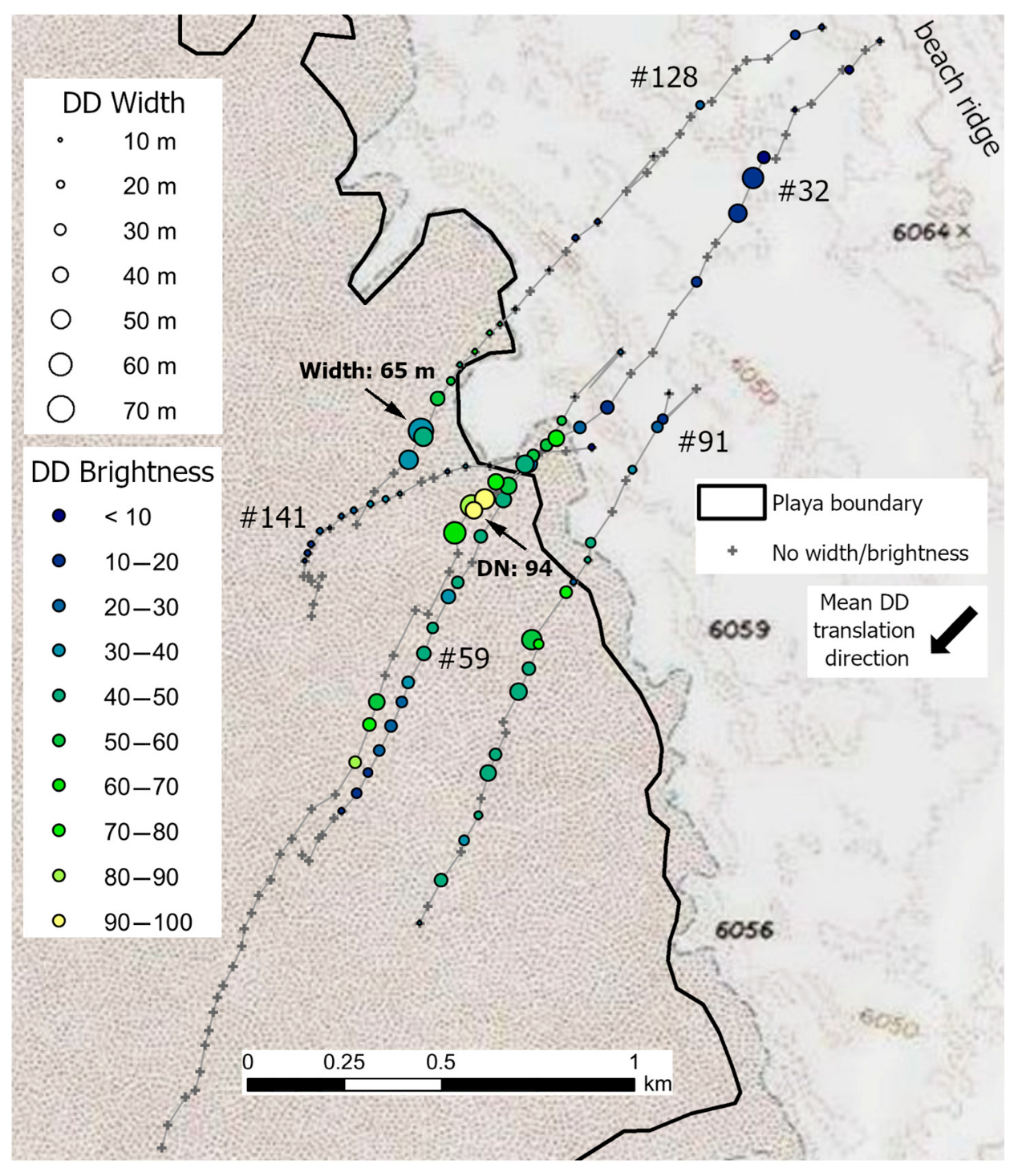
The spatial distribution of DD width and brightness south of the beach ridge shows that the widest and brightest cases occurred on the main playa (Figure S12). This is perhaps best illustrated by isolating long DD sequences (duration > 8 min) that crossed from the phreatophytic hummocky area onto the main playa, with at least three instances observed in each location (Figure 10). In each of these DD sequences, the DD grew in both size and brightness once it crossed onto the bare playa surface. These include two of the longest DD sequences in the dataset, both of which initiated just south of the beach ridge (DD Sequences #32 and #128, which traveled 2.48 km and 1.23 km, for a duration of 18:20 and 10.33 min, respectively). DD Sequence #32 contains the brightest DD instance measured (DN 94, with a corresponding width of 44 m, at 10:48:54), and DD Sequence #128 contains the largest DD width measured (65 m, with a corresponding brightness of DN 37, at 11:30:54). Both instances occurred shortly after these DDs traversed onto the main playa. We infer that the transition onto the main playa may enhance both DD width and brightness.

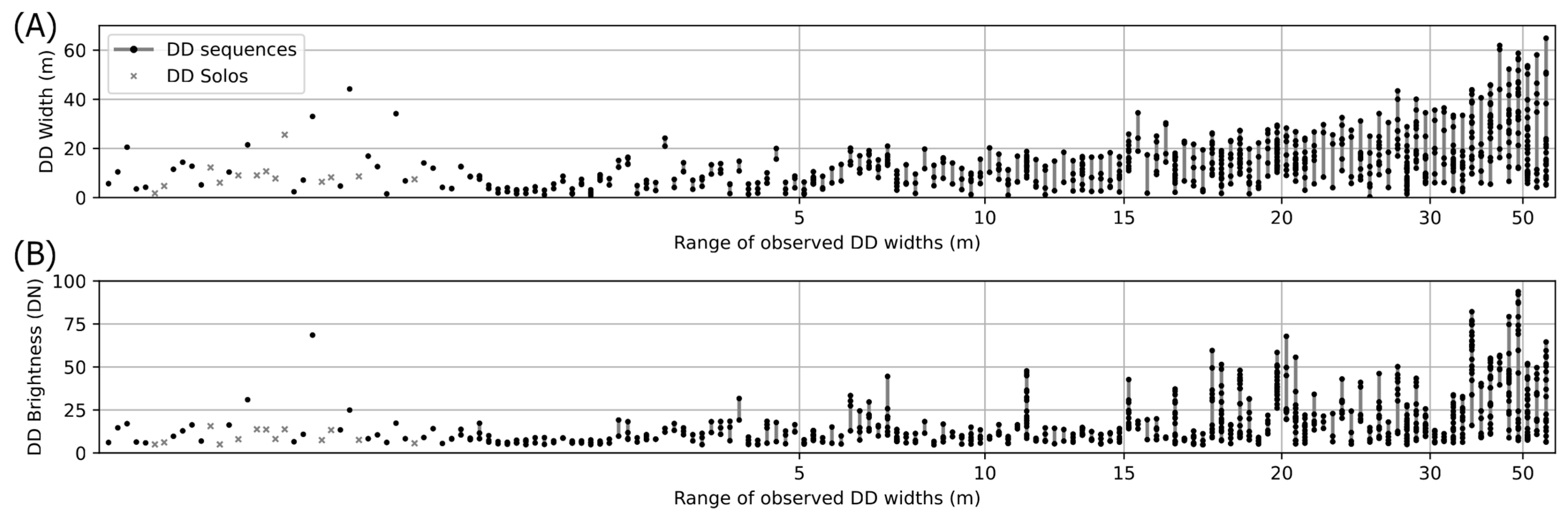
The observed changes in DD width and brightness along the sequences in Figure 10 suggest that some DDs vary considerably in their physical properties as they develop. Figure 11 shows the range of widths and brightnesses for each DD sequence with successful measurements, sorted by the width range. Narrower and dimmer DDs on the left side of the plots generally appear to remain within a typical range, varying by less than 20 m in width and less than 20 in brightness. In contrast, the widest and brightest DD instances belong to DD sequences in which the DDs also experience relatively narrow and dim periods, respectively. This temporal variation may influence the use of single instance width measurements to estimate DD duration (e.g., [41]), because a single image of a DD may not reflect how its properties may vary over time. Some factors, such as crossing onto the main playa, appear to enable DDs to grow in size and opacity. DD Sequences #32 and #128 may have been additionally enhanced (or initiated) by the beach ridge. DDs in longer sequences are more likely to increase in size and brightness, perhaps because any encountered enhancement process also increases the stability of the convective vortex, or perhaps because these convective vortices initiated with a higher vorticity and were able to last long enough to undergo enhancement.

4.2.3. DDs with Tight Cylindrical Morphology

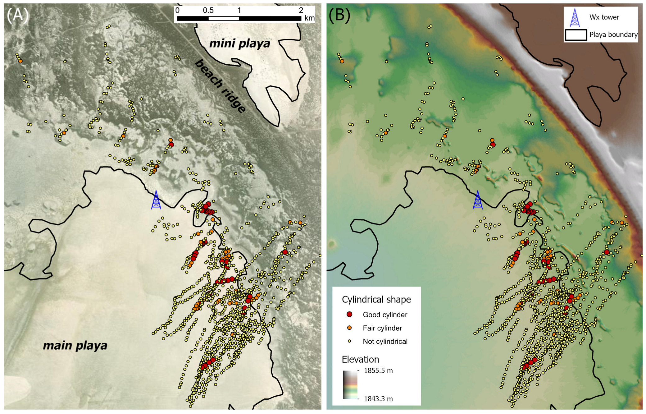
Of the 1230 DD instances with attempted width and brightness measurements located south of the beach ridge, 82 (6.6%) had either a ‘good’ or ‘fair’ cylindrical shape (i.e., ‘Cylindrical’ values of 1 or 2, respectively), and of these only 40 had a ‘good’ cylindrical shape (3.3%). This is similar to the low proportion of sharply defined columns (<4%) and even more rare ‘rope’-shaped columns of DDs observed in the Eldorado Valley, Nevada by [55]. The rarity of these instances suggests that specific conditions must be met for DDs to produce and maintain this form. Comparison of cylindrical forms with other measurements reveals a few characteristics typical of these DDs (Figure S13). The cylindrical form tended to take shape for brief periods during a DD sequence, rarely maintaining this form for more than 2 min, and more often doing so for less than 1 min (Figure S13A,D). Tight cylinders are not typically the first observed shape of a DD sequence, mainly because at initiation, DDs have yet to loft a coherent dust column high enough to be identified as cylindrical. Cylindrical DD instances span the observed range of measured widths and brightnesses (Figure S13B), although few ‘good’ cylindrical instances had brightness DN values less than 10. This is reflected in median values: for ‘good cylindrical’, ‘fair cylindrical’, and all DD instances in Figure S13B, the median brightness is 21, 14, and 13, respectively; and the median widths are 14 m, 8 m, and 11 m, respectively. The higher brightness values of good cylindrical DDs may reflect a subjective bias, as dust column shape is more readily identified in optically thick DDs. Larger ‘good cylinder’ widths occur when these measurements represent the size of the entire DD dust cloud, which was often wider than the tight central cylinder (e.g., Figure 5A). Cylindrical forms occurred throughout the study period, although ‘good’ cylinders formed only after 11:00 (Figure S13C). Finally, there is no apparent correlation with DD duration (Figure S13D), such that cylindrical forms occurred in both short- and long-lived DD sequences.

Considering their spatial distribution, most cylindrical DDs formed on the main playa, in accordance with the overall high number of DDs identified on the playa (Figure 12), and like similar observations from Eldorado Valley [55]. Those DDs that formed in the phreatophytic hummocky area between the main playa and beach ridge most often did so in bright, low-lying areas between the hummocks where playa sediment had begun to accumulate and shrub density was relatively low. As with DD width and brightness, the occurrence of a cylindrical shape is correlated with playa-like surfaces.

4.2.4. Comparison with Meteorological Data

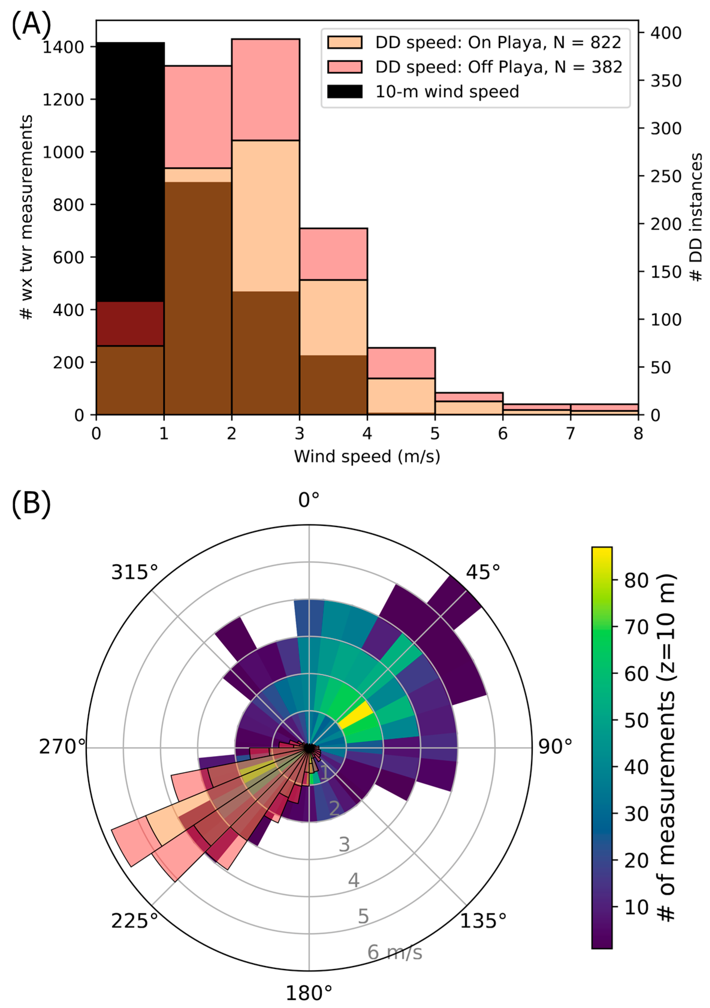
The weather tower obtained 2 s measurements throughout the day, with 2991 measurements occurring between the onset of DD activity and the end of the study period. During this time, winds measured at a height of 10 m were light with a mean speed of 1.35 ± 0.96 m/s (Figure 13A). Mean and modal wind directions were both northeasterly (42 ± 75°) (Figure 13B). DD translation speeds and directions were calculated for each instance, and grouped by their location south of the beach ridge: either on the bare playa or on the vegetated hummocky are. The mean DD translation speed south of the beach ridge, 2.56 ± 1.74 m/s, was 1.9 times greater than the mean 10 m wind speed measured by the meteorological tower. Most DDs translated toward the southwest (228 ± 44°), pushed downwind by the northeasterly wind (42 ± 75°). There was no significant difference in the mean speed or direction of DDs on the playa and hummocky area, although the standard deviation of both speed and direction is higher in the hummocky area than on the playa. The rough surface may lead to greater variation in DD velocities, although we note that the standard deviation would also be increased because (1) DDs on the hummocky region were farther from the cameras and thus had slightly larger location errors, and (2) fewer instance speeds were calculated on the hummocky area.

Figure 14 shows DD activity when compared to some of the measurements derived from the weather tower and ceilometer, described by [43]. Here, we consider which portion of the study area the weather tower instruments sampled. In any given moment, eddy momentum and heat fluxes measured by weather tower instruments represented an adjacent upwind area (i.e., the ‘flux footprint’), the size of which varied with mean wind speed and static stability (e.g., [61]). During the study period, 90% of the measured fluxes represent upwind conditions within a few hundred meters of the tower, most of which is contained in the phreatophytic hummocky area outside the margin of the bare playa. The study period is sufficiently short that only a handful of DDs were observed within the approximate flux footprint, so here we consider DD activity within 1 km of the weather tower (~3 times the upwind length of the flux footprint). Over our study period, 219 DD instances consisting of portions of 26 DD sequences passed within 1 km, and largely upwind, of the weather tower and ceilometer. Similarly to those shown in Figure 13, the DDs near the weather tower translated faster than ambient 10 m winds (2.4 ± 2 m/s, 1.8 times faster) and downwind of the most frequent winds (210 ± 55°).

The first DD to form within 1 km of the meteorological instruments was a solo sighting at 10:36:34, more than 16 min after the first DD was observed elsewhere in the study area. The timing of this nearby sighting corresponds well to meteorological measurements indicating a sharp increase in turbulence kinetic energy (TKE) from 10:30 to 10:45. This sudden increase in TKE was driven by both buoyancy and shear production, as shown, respectively, by increases in eddy heat flux and friction speed (Figure 14B,C). The relative delay in DD onset in the vicinity of the weather tower suggests that conditions conducive to DD formation elsewhere in the study area were reached several minutes prior to those at the weather tower. We note that the friction speed and 10 m wind speed do not correlate well, other than both exhibiting a net increase after 10:30. Assuming that eddy covariance analysis properly de-spiked, de-trended, and tilt-corrected the sonic anemometer data [43], we suspect that these variations are caused by short-term variations in turbulence that the cup anemometer used to measure 10 m wind speeds could not resolve.

Near the weather tower, DD activity fluctuated but generally climbed from 10:45–12:00 local time (Figure 14A). This result contrasts with the observed decrease in DD activity in the broader region south of the beach ridge from 11:30–12:00, as well as the net decrease in TKE from 10:45–12:00. It is unclear whether the observed DD counts near the weather tower were too low to statistically reflect changing environmental conditions, or whether the decrease in TKE within the weather tower’s flux footprint was represented by the regional decrease in DD occurrences. Longer observation times are required to provide more robust statistics of these patterns.

5. Discussion

5.1. What Even Is DD Diameter?

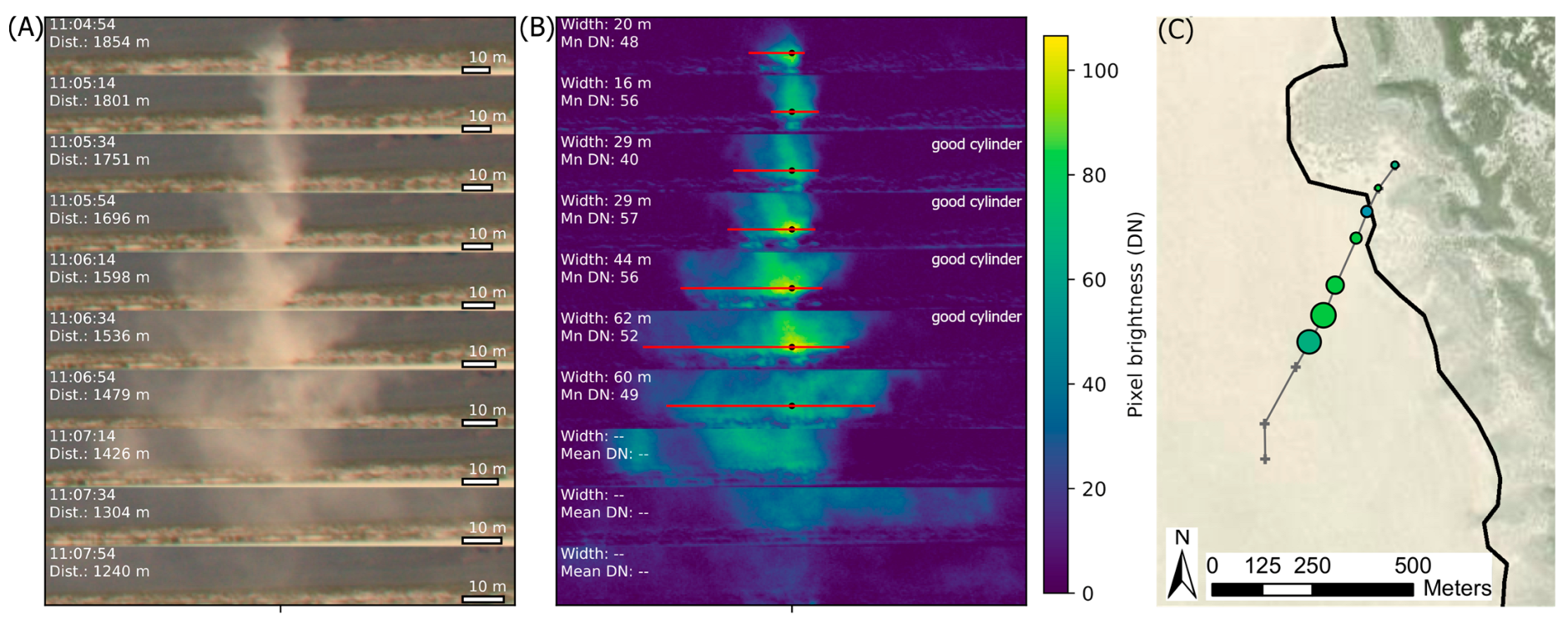
DD width measurements in this study reflected the near-surface, continuous horizontal concentration of dust that could be detected above background noise (Section 3.2.2). In some cases, this measurement represented the apparent extent of the rotational core of the DD, where most visible dust was contained within the rotating column. However, this was not the case for all DDs, with an example shown in Figure 15. This DD began as a short conical wedge of dust (11:04:54) that rapidly elongated vertically (11:05:14). Some dust escaped the rotational central region, spreading laterally, while the core took on a distinctly (‘good’) cylindrical shape (11:05:14–11:06:34, see also Figure 5A). At 11:06:54 the cylindrical core weakened, and dust continued to spread horizontally while the dust plume translated downwind—likely still exhibiting some degree of rotation, but not sufficient to loft more dust. Note that the width measurements do not represent the ‘good’ cylindrical core, but rather the full horizontal extent of the enveloping dust plume. A contrasting example is shown in Figure S14, in which DD Sequence #98 exhibited an opaque dusty column that varied between 10 and 40 m in width over a period of five minutes before dispersing and broadening beyond measurement capability (note that at 11:10:34 an instance of this DD sequence is used as the ‘fair cylindrical’ example in Figure 5B). In this latter example sequence, the measured width may indeed reflect the diameter of the rotational core, or there may be a smaller rotating core that is too heavily obscured by dispersing dust to be identified. Likely, both possibilities play varying roles throughout the duration of this and many other sequences.

In previous field studies, most visual DD width measurements have been based on images or in situ inspection of a short portion of a DD sequence’s duration (e.g., [22,39,62,63,64,65]). In most cases, widths/diameters are listed without description of the criteria used for their measurement, no description of how or whether the rotating core was distinguished from more widely dispersed dust, and little discussion of how individual DD widths varied during a DD’s lifetime. Exceptions include [66], who measured the width of the “core diameter” inside of the “dust diameter”, and [50], who did the opposite and measured the width of the diffuse “outer column” of dust rather than its “well-defined central column”. The restriction to “core diameter” by [66] may in part explain why a similar measure of DD widths in Gusev crater on Mars from the rover Spirit [67] appeared to be larger than their terrestrial counterparts—in addition to other factors [59].

The measurement of DD width from orbital images (mainly of Mars) is likewise varied in methodology, ranging from methods that were not described in detail [68,69,70,71], to those that used the less foreshortened and more distinct shadows [72], to those that avoided the difficulty of near-surface width measurements by measuring the top of the dust plume instead [73]. The earliest of these measurements were greatly limited by camera resolution [68], which has been shown to influence DD width measurements [70]. DDs measured from orbital images are expected to be larger than those measured from surface observations, not only because images from orbit sample a wider area over which less frequent, wide DDs may be found, but also because orbital images are less able to resolve the smaller DDs visible from the ground [59]. Here, we suggest that an additional complication may be that the enveloping dust plume can be indistinguishable from the full rotating DD core at the distance of an orbiting camera. Quantifying this potential discrepancy would require an investigation comparing field images of DD widths to those measured from orbital images. Ideally, this would be conducted both on Earth and Mars, to determine whether the dispersion of dust is similar in the environment of both planets.

DD width has been proposed to be related to convective conditions and has been considered (1) proportional to the Monin–Obukhov length [3,4,74], (2) inversely proportional to the sensible heat flux and the DD’s thermodynamic efficiency [60], (3) related to the lapse rate between heights of 0.3 and 10 m [75], or (4) to represent some fraction of the planetary boundary layer height [59,76]. In the first two cases, DDs would become narrower at peak heating hours (just after noon) when, for example, the Monin–Obukhov length should be at its daily minimum and eddy heat flux is at a maximum. In the last case, DDs should grow rapidly in diameter in the morning and then remain wide until the convective boundary layer collapses in late afternoon. In contrast to these predictions, some studies suggest that DDs reach peak widths at midday [39,63,67]. Our results (Figure 9B) span the rapid CBL growth of the morning, yet the spread in measurements is considerable. The peak mean width occurs between 10:45 and 11:15, coinciding with a sudden rise in the CBL height (Figure 14C) and following the initial burst of convective conditions from 10:30 to 10:45 (Figure 14B,C). The mean widths do indeed drop as noon approaches, consistent with a drop in the Monin–Obukhov length and peak in eddy heat flux (Figure 14C). However, spatial variations in factors affecting DD width obscure this potential relationship (see the following section), such that our data cannot robustly support any of the proposed relationships. The field data required to test any of the hypotheses regarding DD widths includes observations over a spatially uniform area to isolate the atmospheric, and rule out any surface, factors that can also affect DD size.

5.2. Spatial Variations in DD Characteristics: Initiation, Width, Brightness, and Shape

Several previous field studies have identified spatial variations in DD occurrence and their areal density. DDs preferentially form in dry river beds (e.g., [38,55,57,63]), on roads and gravel parking lots [39], where vegetation is limited [51,77], by surface boundaries [40], and over low thermal inertia regions on Mars [15]. Pressure drops diagnostic of convective vortices demonstrate that the vortices themselves, whether they are dust-filled or not, also vary in occurrence spatially [56]. These observations are consistent with the proposal by [63] that DDs most readily form where sediment availability is high, the local ground is anomalously hot, and either local obstructions or terrain boundaries perturb the flow sufficiently to either create vortices or enhance extant ones.

Surface roughness is likely to influence vortex dynamics, but different studies have produced varied results [7]. Large eddy simulations (LES) suggest that rough surfaces should produce more conical-shaped DDs, whereas DDs on smooth surfaces might be more cylindrical [78,79], and this is supported by some field observations (e.g., [7,55]). Our results are also consistent with this trend, with DDs preferentially forming into tight cylinders on smooth, playa-like surfaces. However, the small fraction of these distinctive forms among all those observed has yet to be explained. It appears that some local set of conditions must be met for a DD to form and maintain a tight cylindrical shape.

The role of <1 km scale topography influencing DDs has not been thoroughly investigated in the field [6], likely because DDs are most readily observed and studied on open, flat plains [17,57]. Likewise, numerical models, such as large eddy simulations (LES), are generally idealized with periodic boundary conditions and cannot typically use realistic topography to study its effect on convective vortices [12]. However, theory indicates that a rise in elevation should enhance convective circulations [80]. In contrast, ref. [63] noted that DDs were more prevalent downwind of small mountains, suggesting that the drop in elevation may have created turbulent eddies that contributed to DD formation. At our field site and during the hours of observation investigated here, convecting air advected over a rough alluvial plain, up a 4 m high beach ridge aligned perpendicular to the flow, and then back down a gradual 9 m drop over terrain alternating between vegetated hummocks and low smooth playa-like hollows (Figure 1C). Unstable air impinging on the sunlit, NE side of the beach ridge would undergo vertical acceleration (e.g., [80]). Rotational components of thermals traversing over this ridge might stretch or detach, which could enhance or disrupt these convective vortices, respectively. We suggest that both events occur. Upon acceleration up the beach ridge slope, weak vortices could stretch to the point of being detached, which would explain why no DDs cross over the ridge. In contrast, stronger vortices could strengthen as they are stretched (without being detached), as vertical acceleration intensifies vorticity. This may be how DD Sequences #32 and #128 formed, as they are among the longest-lived, wider, and dustier examples, and both initiated just south of the beach ridge (see Figure 10).

We find that DD occurrence, width, and dust opacity were generally enhanced for those that either formed on or translated onto both the mini playa and the main playa. When transitioning to the playa at SCV, convective structures in the PBL experienced the abrupt influence of (1) a drop in aerodynamic surface roughness by several orders of magnitude [43], (2) a drop in vegetation, (3) an increase in albedo, (4) a decrease in sand availability with which to entrain dust through saltation, and, (5) as a result of increased ground moisture, an increase in thermal conductivity (Figure 1, [43]). These factors are enmeshed and difficult to isolate, given the short observation period considered here.

Although several of the factors listed above should limit DD generation on the playa surface relative to nearby vegetated surfaces, we observed nearly equal rates of DD initiation on and off the playa (Section 4.2.1, Figure S11). In principle, an increase in surface albedo and thermal conductivity would limit playa surface heating and lower the eddy heat flux relative to the vegetated surfaces upwind, slowing CBL growth and weakening thermal updrafts over the playa. Further, development of an ‘offshore’ playa breeze (e.g., [81]) would produce sinking motion over the playa, further inhibiting DD development [82]. Higher surface roughness from vegetation would generate more turbulence than a smooth surface, leading to higher eddy heat fluxes above the vegetated ground [83], which could enhance DD production there. However, several other factors could readily counteract these effects. For example, [51] argued that because roughness from vegetation would also increase friction speed, surface winds would weaken, which would in turn limit DD production over rough surfaces because DDs are not observed to form at low background wind speeds. This is supported by [84], whose lab study also found that rough surfaces resulted in weaker vortices. In addition, although surface roughness generally enhances heat transfer, pockets of cool or warm air trapped in roughness elements (e.g., vegetation) could suppress eddy heat fluxes [85]. Further, any ‘offshore’ playa breeze formed during the period of our study would be southwesterly, counteracting the northeasterly mean flow (Figure 13B). If it is strong enough, the front of this breeze would interact with the mean flow, potentially producing new vertical eddies that could be drawn into nearby thermals, which could in turn lead to more DDs forming as these thermals traverse onto the bare playa surface. All these factors, and perhaps others, worked to create the observed DD behavior. Isolating the effects of any of these conditions may only be possible through investigation of the larger dataset obtained at SCV.

5.3. DD Translation Speed

We measured mean DD translation speeds that were 1.8 times greater than the measured 10 m wind speeds for DD sequences within 1 km of the weather tower (1.9 times for all DD instances south of the beach ridge). This mixed-layer to surface-layer speed ratio (referred to here as ‘MLSL ratio’) is substantially higher than that measured by [50], who found a ratio of ~1.1–1.2 for study areas in Eloy, Arizona and Eldorado Valley, Nevada. It is also higher than the MLSL ratio of ~1 found by [86] near Mopipi, Botswana. Because DDs travel at the height-averaged wind speed of the mixed layer in which their thermal plume hosts are situated [87], their translation speed relative to the near-surface wind reflects the degree of surface layer shear. As a result, DDs are expected to translate faster than the near-surface wind [87]. Because DD motion can be measured in places where no instruments are available to make meteorological measurements, such as on Mars [70,88,89], DD translation speeds are potentially valuable for remotely determining wind speeds. Understanding the range and variability of the MLSL ratio is necessary before this method can be used reliably.

It is unclear why our MLSL ratio is higher than previous measurements [50,86]. We propose two possible explanations for our differing results. First, our study spans less than two hours of DD activity, whereas the two other studies encompass several days of DD production under varying weather conditions. It is possible that the MLSL ratio varies with meteorological conditions, and that our data represents only a small portion of typical convective conditions. Second, our study site is situated ~1300 m higher than that of [50] and ~950 m higher than that of [86]. The lower air density at high elevations affects CBL growth (e.g., [90]), dampens DD production (e.g., [91]), and as we suggest here, may also increase the ratio of the mixed-layer to surface-layer wind speeds.

6. Conclusions

We have analyzed stereo timelapse images of DDs in Smith Creek Valley in central Nevada, USA over a short period ranging from 10:20 to 12:00 local time, capturing the morning growth of the CBL. The study period is a small portion of a multiple-week, interannual field study monitoring weather conditions and DD activity [43]. In this limited sample, 1786 DD instances were located through stereogrammetric triangulation. By comparing one camera frame timestep to another, DD instances were manually organized into 245 individual DDs, the majority of which were imaged several times as they developed and migrated through camera FOVs. We automated a method to isolate each DD instance and measure its width and brightness, the latter of which we used as a proxy for relative dust opacity. DD shape, whether cylindrical or not, was also noted and tracked. From these measurements, we have identified patterns of DD growth, dust concentration, and shape coherence that correspond to variations in both local meteorology and the surface over which they traverse.

Of the observed 220 DD sequences and 25 solo instances, the mean and maximum durations (2.22 min and 18.33 min, respectively) were similar to those noted in previous DD field studies. Modal DD widths ranged from 10 to 20 m, similar to previous measurements [57]. DDs with widths > 14.4 m fit a differential power law with an exponent of −1.55, smaller than that found in previous datasets [59] but comparable to that theorized by [60]. We note that the statistical significance of our exponent is limited by a short investigation period.

Most unusual was the measured DD translation speed, at ~1.9 times that of the mean wind speed (‘MLSL ratio’), which is much higher than previously measured ratios ranging from 1 to 1.2 [50,86]. Our higher measured MLSL ratio may be the result of our short duration study period, but we also consider that other factors, such as elevation, may influence CBL motions from one study site to another. A better understanding of factors controlling this ratio would help constrain its value for remote determination of mixed layer and surface layer wind speeds.

DDs varied considerably over the study period, and through each DD’s lifetime:

• Wider and dustier DDs were most common just after an initial spike in CBL growth from 10:45 to 11:15. From 11:15 to 11:45, DDs became more numerous (i.e., areally dense), with longer durations. However, the measured DD parameters varied so greatly that these apparent temporal patterns may not be statistically significant. Regardless, we can assert that the measured DD physical characteristics did not correspond readily with any previously proposed meteorological controls (e.g., Monin–Obukhov length, sensible heat flux, lapse rate, CBL height). The only consistent controls in this study appear to have been variations in surface properties, which dominated over atmospheric variations. Isolating any atmospheric forcing will require investigating DD characteristics over a uniform surface.
• Wide, dusty, and strongly cylindrical DDs tended to exhibit these characteristics for only a short portion of a DD sequence’s duration, and not always at the same time. For example, DDs with narrow, crisp-edged cylindrical shapes typically appeared this way for <1 min, dissipating to less well-organized, diffuse dust columns for the remainder of their durations. This finding indicates that an instantaneous observation of a large, optically thick, or coherently shaped DD should not be used to extrapolate values (e.g., vertical dust fluxes) over the DD’s duration.

DD activity was not spatially uniform in the study area:

• Although the first DD sighting at SCV occurred at 10:20:14, the first DD observed within 1 km of the weather tower appeared at 10:36:34, 16.33 min later. The delayed onset of DD activity in the vicinity of the weather tower coincided neatly with a measured rise in TKE at 10:30–10:45. The higher albedo and thermal conductivity of the compact playa surface, where the weather tower was located, likely hindered DD production relative to the darker, sandy surface of the vegetated terrain beyond the playa margin.
• Despite DD traverse lengths often exceeding 1 km, DDs were generally not observed to cross a 4 m high beach ridge aligned perpendicular to their translation direction. However, two of the longest and most intense DD sequences initiated just downwind of this ridge. We propose that convective vortices impinging on the beach ridge are vertically stretched as winds accelerate up the ridge slope, concentrating vorticity. This could cause weaker vortices to detach from the surface, preventing DDs from forming along the ridge. In contrast, stronger vortices would be further strengthened by increased vertical winds, such that strong DDs could form under the same conditions that suppress weaker vortices.
• Although DDs were plentiful in the vegetated, hummocky area between the playas, these DD sequences tended to be shorter, less dusty, and narrow. DDs that either initiated on or traversed onto the playa surface tended to last longer, and the widest and dustiest DD instances corresponded with DDs that had just entered the main playa. The bare playa, as well as the transition to it, enhanced DD stability, size, and dust lofting capability. This may occur for numerous reasons, as convective structures experienced an abrupt transition in surface properties as they crossed from the vegetated, hummocky area to the bare playa, including surface roughness, transpiration, albedo, sediment availability, and thermal conductivity. Further investigation of the broader field data could isolate some of these factors, e.g., investigating DD characteristics when the wind blows from other directions.

Finally, we consider a caveat regarding DD width measurements. Dust is often flung laterally from the DD’s rotational core, potentially obscuring this core with an enveloping dust plume. Field studies and orbital image studies have measured DD widths in different ways, and most did not describe their methodology: did width measurements include the envelope or the central core, and what criteria were established for determining the rotational margin of a DD? In our images, we defined DD width as the extent of contiguous horizontal image pixels with brightnesses above the differenced background median plus median absolute deviation (Figure 4D), resulting in a semi-automated method that may or may not include portions of an enveloping dust plume, which may or may not be present. The various methods in the literature are likely to have led to variations in DD size statistics, which in turn prevent determination of any relationship between DD width—and thus vertical dust flux—and local environmental conditions. We encourage detailed descriptions of width determination methods, and use of consistent criteria for measuring DD widths.

This investigation found that DDs are fitful phenomena that are difficult to measure consistently and are strongly controlled by the properties of the surface they traverse. As the poet Propertius said, formosis levitas semper amica fuit, “fickleness has always befriended the beautiful” (Elegies II, c. 25 BCE). Although this study was limited to less than two hours of DD activity, our results demonstrate that it is possible to analyze DD physical characteristics with partial automation. The measurements presented here would serve well as training data for use with machine learning methods on the broader field campaign data.

References

1. Young, G. Convection in the atmospheric boundary layer. Earth Sci. Rev. 1988, 25, 179–198. [Google Scholar] [CrossRef]
2. Willis, G.E.; Deardorff, J.W. Laboratory observations of turbulent penetrative-convection planforms. J. Geophys. Res. 1979, 84, 295–302. [Google Scholar] [CrossRef]
3. Hess, G.D.; Spillane, K.T. Characteristics of dust devils in Australia. J. Appl. Meteorol. 1990, 29, 498–507. [Google Scholar] [CrossRef] [PubMed]
4. Kanak, K.M.; Lilly, D.K.; Snow, J.T. The formation of vertical vortices in the convective boundary layer. Q. J. R. Meteorol. Soc. 2000, 126, 2789–2810. [Google Scholar] [CrossRef]
5. Raasch, S.; Franke, T. Structure and formation of dust devil–like vortices in the atmospheric boundary layer: A high-resolution numerical study. J. Geophys. Res. 2011, 116, D16120, 1–16. [Google Scholar] [CrossRef]
6. Rafkin, S.; Jemmett-Smith, B.; Fenton, L.; Lorenz, R.; Takemi, T.; Ito, J.; Tyler, D. Dust devil formation. Space Sci. Rev. 2016, 203, 183–207. [Google Scholar] [CrossRef]
7. Kurgansky, M.V.; Lorenz, R.D.; Renno, N.O.; Takemi, T.; Gu, Z.; Wei, W. Dust Devil Steady-State Structure from a Fluid Dynamics Perspective. Space Sci. Rev. 2016, 203, 209–244. [Google Scholar] [CrossRef]
8. Dahl, J.M.L. The Development of Simulated Dust-Devil-Like Vortices. J. Atmos. Sci. 2024, 81, 1883–1899. [Google Scholar] [CrossRef]
9. Toigo, A.D.; Richardson, M.I. Meteorology of proposed Mars Exploration Rover landing sites. J. Geophys. Res. 2003, 108, 8092. [Google Scholar] [CrossRef]
10. Kanak, K.M. On the numerical simulation of dust devil–like vortices in terrestrial and Martian convective boundary layers. Geophys. Res. Lett. 2006, 33, L19S05, 1–4. [Google Scholar] [CrossRef]
11. Spiga, A.; Forget, F. A new model to simulate the Martian mesoscale and microscale atmospheric circulation: Validation and first results. J. Geophys. Res. 2009, 114, E02009, 1–26. [Google Scholar] [CrossRef]
12. Spiga, A.; Barth, E.; Gu, Z.; Hoffmann, F.; Ito, J.; Jemmett-Smith, B.; Klose, M.; Nishizawa, S.; Raasch, S.; Rafkin, S.; et al. Large-Eddy Simulations of Dust Devils and Convective Vortices. Space Sci. Rev. 2016, 203, 245–275. [Google Scholar] [CrossRef]
13. Wu, Z.; Richardson, M.I.; Zhang, X.; Cui, J.; Heavens, N.G.; Lee, C.; Li, T.; Lian, Y.; Newman, C.E.; Soto, A.; et al. Large Eddy Simulations of the Dusty Martian Convective Boundary Layer with MarsWRF. J. Geophys. Res. Planets 2021, 126, e2020JE006752. [Google Scholar] [CrossRef]
14. Spiga, A.; Murdoch, N.; Lorenz, R.; Forget, F.; Newman, C.; Rodriguez, S.; Pla-Garcia, J.; Viúdez Moreiras, D.; Banfield, D.; Perrin, C.; et al. A Study of Daytime Convective Vortices and Turbulence in the Martian Planetary Boundary Layer Based on Half-a-Year of InSight Atmospheric Measurements and Large-Eddy Simulations. J. Geophys. Res. Planets 2021, 126, e2020JE006511. [Google Scholar] [CrossRef]
15. Hueso, R.; Newman, C.E.; del Río-Gaztelurrutia, T.; Munguira, A.; Sánchez-Lavega, A.; Toledo, D.; Apéstigue, V.; Arruego, I.; Vicente-Retortillo, A.; Martínez, G.; et al. Convective Vortices and Dust Devils Detected and Characterized by Mars 2020. J. Geophys. Res. Planets 2023, 128, e2022JE007516. [Google Scholar] [CrossRef]
16. Fenton, L.; Reiss, D.; Lemmon, M.; Marticorena, B.; Lewis, S.; Cantor, B. Orbital observations of dust lofted by daytime convective turbulence. Space Sci. Rev. 2016, 203, 89–142. [Google Scholar] [CrossRef]
17. Murphy, J.; Steakley, K.; Balme, M.; Deprez, G.; Esposito, F.; Kahanpää, H.; Lemmon, M.; Lorenz, R.; Murdoch, N.; Neakrase, L.; et al. Field measurements of terrestrial and martian dust devils. Space Sci. Rev. 2016, 203, 39–87. [Google Scholar] [CrossRef]
18. Jackson, B.; Lorenz, R.D.; Barnes, J.W.; Szurgot, M. Dust Devils on Titan. J. Geophys. Res. Planets 2020, 125, e2019JE006238. [Google Scholar] [CrossRef]
19. Spiga, A.; Lefèvre, M.; Vatant d’Ollone, J.; Lebonnois, S.; Rodriguez, S.; Chatain, A.; Bonnefoy, L. Developping a new model for mesoscale and large-eddy simulations of Titan’s atmosphere. In Proceedings of the Europlanet Science Congress, Virtual, 21 September–9 October 2020. [Google Scholar] [CrossRef]
20. Lavely, A.; Lorenz, R.; Schmitz, S. Large-Eddy Simulation of Titan’s near-surface atmosphere: Convective turbulence and flow over dunes with application to Huygens and Dragonfly. Icarus 2021, 357, 114229. [Google Scholar] [CrossRef]
21. Rafkin, S.; Soto, A.; Chin-Canche, G. The structure and evolution of Titan’s daytime planetary boundary layer. In Proceedings of the Europlanet Science Congress, Berlin, Germany, 8–13 September 2024. [Google Scholar] [CrossRef]
22. Flower, W.D. Sand devils. London Meteorol. Off. Prof. Notes 1936, 5, 1–16. [Google Scholar]
23. Jemmett-Smith, B.C.; Marsham, J.H.; Knippertz, P.; Gilkeson, C.A. Quantifying global dust devil occurrence from meteorological analyses. Geophys. Res. Lett. 2015, 42, 1275–1282. [Google Scholar] [CrossRef] [PubMed]
24. Klose, M.; Shao, Y. A numerical study on dust devils with implications to global dust budget estimates. Aeolian Res. 2016, 22, 47–58. [Google Scholar] [CrossRef]
25. Gillette, D.A.; Sinclair, P.C. Estimation of suspension of alkaline material by dust in the United States. Atmos. Environ. 1990, 24A, 1135–1142. [Google Scholar] [CrossRef]
26. Klamt, J.; Giersch, S.; Raasch, S. Saltation-induced dust emission of dust devils in the convective boundary layer—An LES study on the meter scale. J. Geophys. Res. Atmos. 2024, 129, e2023JD040058. [Google Scholar] [CrossRef]
27. Yang, X.; Ma, M.; Zhou, C.; Yang, F.; Huo, W.; Mamtimin, A.; He, Q.; Wang, G. Contributions of dust and non-dust weather to dust emissions: A case study from the central Taklimakan Desert. Remote Sens. 2025, 17, 2531. [Google Scholar] [CrossRef]
28. Takemi, T.; Yasui, M.; Zhou, J.; Liu, L. Role of boundary layer and cumulus convection on dust emission and transport over a midlatitude desert area. J. Geophys. Res. Atmos. 2006, 111, D11203. [Google Scholar] [CrossRef]
29. Engelstaedter, S.; Washington, R. Atmospheric controls on the annual cycle of North African dust. J. Geophys. Res. 2007, 112, D03103. [Google Scholar] [CrossRef]
30. Marsham, J.H.; Parker, D.J.; Grams, C.M.; Johnson, B.T.; Grey, W.M.F.; Ross, A.N. Observations of mesoscale and boundary-layer scale circulations affecting dust transport and uplift over the Sahara. Atmos. Chem. Phys. 2008, 8, 6979–6993. [Google Scholar] [CrossRef]
31. Han, Y.; Wang, K.; Liu, F.; Zhao, T.; Yin, Y.; Duan, J.; Luan, Z. The contribution of dust devils and dusty plumes to the aerosol budget in western China. Atmos. Environ. 2016, 126, 21–27. [Google Scholar] [CrossRef]
32. Ju, T.; Li, X.; Zhang, H.; Cai, X.; Song, Y. Parameterization of dust flux emitted by convective turbulent dust emission (CTDE) over the Horqin Sandy Land area. Atmos. Environ. 2018, 187, 62–69. [Google Scholar] [CrossRef]
33. Tang, Y.; Han, Y.; Liu, Z. Temporal and spatial characteristics of dust devils and their contribution to the aerosol budget in East Asia—An analysis using a new parameterization scheme for dust devils. Atmos. Environ. 2018, 182, 225–233. [Google Scholar] [CrossRef]
34. Ma, M.; Yang, X.; He, Q.; Zhou, C.; Mamtimin, A.; Huo, W.; Yang, F. Characteristics of dust devil and its dust emission in northern margin of the Taklimakan Desert. Aeolian Res. 2020, 44, 100579. [Google Scholar] [CrossRef]
35. Pan, L.; Han, Y.; Lu, Z.; Li, J.; Gao, F.; Liu, Z.; Liu, W.; Liu, Y. Integrative investigation of dust emissions by dust storms and dust devils in North Africa. Sci. Total Environ. 2021, 756, 144128. [Google Scholar] [CrossRef] [PubMed]
36. Kok, J.F.; Adebiyi, A.A.; Albani, S.; Balkanski, Y.; Checa-Garcia, R.; Chin, M.; Colarco, P.R.; Hamilton, D.S.; Huang, Y.; Ito, A.; et al. Improved representation of the global dust cycle using observational constraints on dust properties and abundance. Atmos. Chem. Phys. 2021, 21, 8127–8167. [Google Scholar] [CrossRef] [PubMed]
37. Leung, D.M.; Kok, J.F.; Li, L.; Okin, G.S.; Prigent, C.; Klose, M.; García-pando, C.P.; Menut, L.; Mahowald, N.M.; Lawrence, D.M.; et al. A new process-based and scale-aware desert dust emission scheme for global climate models—Part I: Description and evaluation against inverse modeling emissions. Atmos. Chem. Phys. 2023, 23, 6487–6523. [Google Scholar] [CrossRef]
38. Sinclair, P.C. A Quantitative Analysis of the Dust Devil. Ph.D. Thesis, University of Arizona, Tucson, AZ, USA, 1966. [Google Scholar]
39. Snow, J.T.; McClelland, T.M. Dust Devils at White Sands Missile Range, New Mexico 1. Temporal and spatial distributions. J. Geophys. Res. 1990, 95, 13707–13721. [Google Scholar] [CrossRef]
40. Renno, N.O.; Abreu, V.J.; Koch, J.; Smith, P.H.; Hartogensis, O.K.; De Bruin, H.A.R.; Burose, D.; Delory, G.T.; Farrell, W.M.; Watts, C.J.; et al. MATADOR 2002: A pilot field experiment on convective plumes and dust devils. J. Geophys. Res. 2004, 109, E07001. [Google Scholar] [CrossRef]
41. Lorenz, R. The longevity and aspect ratio of dust devils: Effects on detection efficiencies and comparison of landed and orbital imaging at Mars. Icarus 2013, 226, 964–970. [Google Scholar] [CrossRef]
42. Neakrase, L.D.V.; Greeley, R.; Iversen, J.D.; Balme, M.R.; Eddlemon, E.E. Dust flux within dust devils: Preliminary laboratory simulations. Geophys. Res. Lett. 2006, 33, L19S09. [Google Scholar] [CrossRef]
43. Fenton, L.K.; Metzger, S.M.; Michaels, T.I.; Scheidt, S.P.; Dorn, T.C.; Neakrase, L.D.V.; Cole, B.; Sprau, O. Meteorological and geological controls on dust devil activity: Initial results from a field study at Smith Creek Valley, Nevada, USA. Aeolian Res. 2022, 59, 100831. [Google Scholar] [CrossRef]
44. Fenton, L.F.; Metzger, S.M.; Scheidt, S.P.; Michaels, T.I.; Dorn, T.C.; Neakrase, L.D.V.; Battin, R.; Cole, B.; Crevier, J.; Idec, E.; et al. Dust devil survey of Smith Creek Playa, Nevada (2019–2021). PDS Atmos. Node. [CrossRef]
45. Crafford, A.E.J. Geologic Map of Nevada; U.S. Geological Survey Data Series; U.S. Geological Survey: Reston, VA, USA, 2007; Volume 249, p. 46.
46. Thomas, J.M.; Carlton, S.M.; Hines, L.B. Ground-Water Hydrology and Simulated Effects of Development in Smith Creek Valley, a Hydrologically Closed Basin in Lander County, Nevada; Professional Paper 1409-E; U.S. Geological Survey: Reston, VA, USA, 1989. [CrossRef]
47. USGS. 3D Elevation Program 1/3 Arc Second Resolution Digital Elevation Model. 2023. Available online: https://www.usgs.gov/the-national-map-data-delivery (accessed on 15 November 2024).
48. Mifflin, M.D.; Wheat, M.M. Pluvial Lakes and Estimated Pluvial Lakes of Nevada; Reno, N.V., Ed.; Nevada Bureau of Mines and Geology, University of Nevada: Reno, NV, USA, 1979; Bulletin 94; 57p. [Google Scholar]
49. Lorenz, R.D.; Jackson, B.; Barnes, J.W. Inexpensive time-lapse digital cameras for studying transient meteorological phenomena: Dust devils and playa flooding. J. Atmos. Ocean. Technol. 2010, 27, 246–256. [Google Scholar] [CrossRef]
50. Balme, M.R.; Pathare, A.; Metzger, S.M.; Towner, M.C.; Lewis, S.R.; Spiga, A.; Fenton, L.K.; Renno, N.O.; Elliott, H.M.; Saca, F.A.; et al. Field measurements of horizontal forward motion velocities of terrestrial dust devils: Towards a proxy for ambient winds on Mars and Earth. Icarus 2012, 221, 632–645. [Google Scholar] [CrossRef]
51. Lyons, T.J.; Nair, U.S.; Foster, I.J. Clearing enhances dust devil formation. J. Arid. Environ. 2008, 72, 1918–1928. [Google Scholar] [CrossRef]
52. Takemi, T. An eddy-resolving simulation of the diurnal variation of fair-weather convection and tracer transport. Atmos. Res. 2008, 89, 270–282. [Google Scholar] [CrossRef]
53. Garnier, S.; Ross, N.; Rudis, R.; Camargo, P.A.; Sciaini, M.; Scherer, C. Viridis(Lite)—Colorblind-Friendly Color Maps for R, version 0.6.5; Zenodo: Geneva, Switzerland, 2024. [Google Scholar] [CrossRef]
54. Lorenz, R.D. Power law of dust devil diameters on Mars and Earth. Icarus 2009, 203, 683–684. [Google Scholar] [CrossRef]
55. Metzger, S.M. Dust Devils as Aeolian Transport Mechanisms in Southern Nevada and the Mars Pathfinder Landing Site. Ph.D. Thesis, University of Nevada, Reno, NV, USA, 1999. [Google Scholar]
56. Jackson, B.; Lorenz, R. A multiyear dust devil vortex survey using an automated search of pressure time series. J. Geophys. Res. 2015, 120. [Google Scholar] [CrossRef]
57. Balme, M.; Greeley, R. Dust devils on Earth and Mars. Rev. Geophys. 2006, 44, RG3003. [Google Scholar] [CrossRef]
58. Lorenz, R. On the statistical distribution of dust devil diameters. Icarus 2011, 215, 381–390. [Google Scholar] [CrossRef]
59. Lorenz, R.D.; Jackson, B.K. Dust Devil Populations and Statistics. Space Sci. Rev. 2016, 203, 277–297. [Google Scholar] [CrossRef]
60. Jackson, B.; Fenton, L.; Lorenz, R.; Szurgot, C.; Gambill, J.; Arzaga, G. On Dust Devil Diameters, Occurrence Rates, and Activity. Planet. Sci. J. 2025, 6, 193. [Google Scholar] [CrossRef]
61. Kljun, N.; Calanca, P.; Rotach, M.W.; Schmid, H.P. A simple parameterisation for flux footprint predictions. Bound.-Layer Meteorol. 2004, 112, 503–523. [Google Scholar] [CrossRef]
62. Williams, N.R. Development of dust whirls and similar small-scale vortices. Bull. Am. Meteorol. Soc. 1948, 29, 106–117. [Google Scholar] [CrossRef]
63. Sinclair, P.C. General characteristics of dust devils. J. Appl. Meteorol. 1969, 8, 32–45. [Google Scholar] [CrossRef] [PubMed]
64. Carroll, J.J.; Ryan, J.A. Atmospheric vorticity and dust devil rotation. J. Geophys. Res. 1970, 75, 5179–5184. [Google Scholar] [CrossRef]
65. Pathare, A.V.; Balme, M.R.; Metzger, S.M.; Spiga, A.; Towner, M.C.; Renno, N.O.; Saca, F. Assessing the power law hypothesis for the size–frequency distribution of terrestrial and martian dust devils. Icarus 2010, 209, 851–853. [Google Scholar] [CrossRef]
66. Ryan, J.A.; Carroll, J.J. Dust devil wind velocities: Mature state. J. Geophys. Res. 1970, 75, 531–541. [Google Scholar] [CrossRef]
67. Greeley, R.; Waller, D.A.; Cabrol, N.A.; Landis, G.A.; Lemmon, M.T.; Neakrase, L.D.V.; Pendleton Hoffer, M.; Thompson, S.D.; Whelley, P.L. Gusev Crater, Mars: Observations of three dust devil seasons. J. Geophys. Res. 2010, 115, E00F02. [Google Scholar] [CrossRef]
68. Thomas, P.; Gierasch, P.J. Dust devils on Mars. Science 1985, 230, 175–177. [Google Scholar] [CrossRef] [PubMed]
69. Stanzel, C.; Pätzold, M.; Greeley, R.; Hauber, E.; Neukum, G. Dust devils on Mars observed by the High Resolution Stereo Camera. Geophys. Res. Lett. 2006, 33, L11202. [Google Scholar] [CrossRef]
70. Stanzel, C.; Patzold, M.; Williams, D.; Whelley, P.; Greeley, R.; Neukum, G.; Team, T.H.C.-I. Dust devil speeds, directions of motion and general characteristics observed by the Mars Express High Resolution Stereo Camera. Icarus 2008, 197, 39–51. [Google Scholar] [CrossRef]
71. Reiss, D. First observations of terrestrial dust devils in orbital image data: Comparison with dust devils in Amazonis Planitia, Mars. In Proceedings of the 47th Lunar and Planetary Sciece Conference, The Woodlands, TX, USA, 21–25 March 2016; Available online: https://www.hou.usra.edu/meetings/lpsc2016/pdf/2912.pdf (accessed on 19 June 2026).
72. Fisher, J.A.; Richardson, M.I.; Newman, C.E.; Szwast, M.A.; Graf, C.; Basu, S.; Ewald, S.P.; Toigo, A.D.; Wilson, R.J. A survey of Martian dust devil activity using Mars Global Surveyor Mars Orbiter Camera images. J. Geophys. Res. 2005, 110, E03004. [Google Scholar] [CrossRef]
73. Conway, S.J.; Bickel, V.T.; Fenton, L.K.; Patel, M.R.; Carson, H.C.; Blouin, A.; Crevier, J.; Blanc, E.; Nguyen, B.N.; Holmes, J.A.; et al. A global survey for dust devil vortices on mars using MRO context camera images enabled by neural networks. Planet. Space Sci. 2025, 259, 106072. [Google Scholar] [CrossRef]
74. Kurgansky, M.V.; Montecinos, A.; Villagran, V.; Metzger, S.M. Micrometeorological conditions for dust-devil occurrence in the Atacama Desert. Bound.-Layer Meteorol. 2011, 138, 285–298. [Google Scholar] [CrossRef]
75. Ryan, J.A. Relation of dust devil frequency and diameter to atmospheric temperature. J. Geophys. Res. 1972, 77, 7133–7137. [Google Scholar] [CrossRef]
76. Lorenz, R.D. An engineering model of Titan surface winds for Dragonfly landed operations. Adv. Space Res. 2021, 67, 2219–2230. [Google Scholar] [CrossRef]
77. Oke, A.M.C.; Tapper, N.J.; Dunkerley, D. Willy-willies in the Australian landscape: The role of key meteorological variables and surface conditions in defining frequency and spatial characteristics. J. Arid. Environ. 2007, 71, 201–215. [Google Scholar] [CrossRef]
78. Zhao, Y.; Gu, Z.; Yu, Y.; Ge, Y.; Li, Y.; Feng, X. Mechanism and Large Eddy Simulation of Dust Devils. Atmos.-Ocean 2004, 42, 61–84. [Google Scholar] [CrossRef]
79. Gu, Z.; Qiu, J.; Zhao, Y.; Li, Y. Simulation of terrestrial dust devil patterns. Adv. Atmos. Sci. 2008, 25, 31–42. [Google Scholar] [CrossRef]
80. Souza, E.P.; Rennó, N.O.; Silva Dias, M.A. Convective circulations induced by surface heterogeneities. J. Atmos. Sci. 2000, 57, 2915–2922. [Google Scholar] [CrossRef]
81. Rife, D.L.; Warner, T.T.; Chen, F.; Astling, E.G. Mechanisms for diurnal boundary layer circulations in the Great Basin Desert. Mon. Weather. Rev. 2002, 130, 921–938. [Google Scholar] [CrossRef][Green Version]
82. Giersch, S.; Brast, M.; Hoffmann, F.; Raasch, S. Toward Large-Eddy Simulations of Dust Devils of Observed Intensity: Effects of Grid Spacing, Background Wind, and Surface Heterogeneities. J. Geophys. Res. Atmos. 2019, 124, 7697–7718. [Google Scholar] [CrossRef]
83. Hang, C.; Nadeau, D.F.; Pardyjak, E.R.; Parlange, M.B. A comparison of near-surface potential temperature variance budgets for unstable atmospheric flows with contrasting vegetation cover flat surfaces and a gentle slope. Environ. Fluid Mech. 2020, 20, 1251–1279. [Google Scholar] [CrossRef]
84. Neakrase, L.D.V.; Greeley, R. Dust devils in the laboratory: Effect of surface roughness on vortex dynamics. J. Geophys. Res. 2010, 115, E05003. [Google Scholar] [CrossRef]
85. Zhang, Y.; Sun, C.; Bao, Y.; Zhou, Q. How surface roughness reduces heat transport for small roughness heights in turbulent Rayleigh—Bénard convection. J. Fluid Mech. 2018, 836, 1–10. [Google Scholar] [CrossRef]
86. Toledo, D.; Apéstigue, V.; Martinez-Oter, J.; Franchi, F.; Serrano, F.; Yela, M.; de la Torre Juarez, M.; Rodriguez-Manfredi, J.A.; Arruego, I. Using the Perseverance MEDA-RDS to identify and track dust devils and dust-lifting gust fronts. Front. Astron. Space Sci. 2023, 10, 1221726. [Google Scholar] [CrossRef]
87. Stull, R.B. An Introduction to Boundary Layer Meteorology; Kluwer Academic Publishers: Dordrecht, The Netherlands, 1988. [Google Scholar]
88. Reiss, D.; Spiga, A.; Erkeling, G. The horizontal motion of dust devils on Mars derived from CRISM and CTX/HiRISE observations. Icarus 2014, 227, 8–20. [Google Scholar] [CrossRef]
89. Bickel, V.T.; Almeida, M.; Read, M.; Schriever, A.; Tirsch, D.; Hauber, E.; Gwinner, K.; Thomas, N.; Roatsch, T. Dust devil migration patterns reveal strong surface winds across Mars. Sci. Adv. 2025, 11, eadw5170. [Google Scholar] [CrossRef] [PubMed]
90. De Wekker, S.F.J.; Kossmann, M. Convective boundary layer heights over mountainous terrain—A review of concepts. Front. Earth Sci. 2015, 3, 77. [Google Scholar] [CrossRef]
91. Wang, M.; Huang, Q.; Du, J.; Liao, H.; Dai, Y. Large eddy simulation study on the structure and evolution of dust devils in the Qaidam Basin. Atmos. Res. 2025, 326, 108324. [Google Scholar] [CrossRef]
Figure 1. The field site, showing (A) regional context in Nevada spanning 117°06′–117° 54′ W, 39°06′–39°36′ N (inset shows the map’s location within the contiguous western US). U.S. Route 50 appears as a yellow line passing through the north end of the valley. Black arrows show prominent Pleistocene beach ridges. The black box provides context for (B), the study area in Smith Creek Valley. Blue icons mark the location of the weather tower and suite of cameras, with their respective camera stations numbered #1 through #4. Blue lines show camera fields of view, fully overlapping on and beyond the north end of the main playa. Map data: Google, ©2025 Airbus. (C) Elevation profile A-A′ (10 m horizontal resolution) crossing from the main playa through the lower reaches of the alluvial plain north of the mini playa (vertical exaggeration: 66×). Elevation data is from [47].
Geosciences 16 00262 g001
Figure 2. (A) Image from Camera Station #1 (11 June 2019 at 11:03:54 local time) that has been contrast-stretched, and (B) difference between the frame at 11:03:54 and the following frame at 11:04:14, highlighting subtle details in lofted and moving dust. Each DD is labeled with an identifier letter, in order from left to right. The difference image is shown with a viridis color palette [53]: DDs in the current timestep appear purple, while those in the following timestep appear yellow. The white arrow points to the dust plume of a car just entering the field of view from the left. The Image ID in the upper left corner corresponds with the filename (e.g., ‘ST015313.CR2’). Views of this timestep from all four cameras are shown in Figures S1 and S2.
Geosciences 16 00262 g002
Figure 3. Horizontal positional uncertainty (σxy) distributions for DD locations derived from multi-view intersections, separated by projection count. Three-projection solutions exhibit low errors and a narrow distribution, while four-projection solutions show decreased uncertainty due to an additional observing camera. Two-projection uncertainty estimates are underdetermined with only single ray intersections. Histograms are clipped to the 95% interval.
Geosciences 16 00262 g003
Figure 4. Measuring DD width and relative brightness. (A) A 400 × 600-pixel image portion, centered on a representative DD. The image was taken by Camera Station #4 at 10:38:54; the DD is from Sequence #27, located 2.5 km from the camera (beyond the margin of the bare playa). The white triangle points to the location of the DD. (B) The same image, with the darkest pixels from the surrounding 6 images subtracted out, leaving behind only features that vary temporally, such as a refracting layer of turbulent, heated air (mirage) and a skyline created as wind buffeted the camera. (C) A portion of the image (outlined in (B)) from which the DD was measured, masking areas outside a 15-pixel high area to ensure a uniformly dark background above the nearby hummocky terrain, and to avoid the mirage layer. (D) Differenced pixel brightness values from 3 image rows surrounding the brightest pixel. DD widths and brightnesses were calculated from the area shown in cyan (also shown in (C)), for which contiguous pixel brightnesses were greater than the median + median absolute deviation (MAD). In this case, the DD width is 40 pixels, equating to a width of 16 m, and a mean relative brightness of 17.
Geosciences 16 00262 g004
Figure 5. Examples of Camera Station #4 images of (A) cylindrical (‘good cylindrical’), (B) somewhat cylindrical (‘fair cylindrical’), and not cylindrical DDs. Cylindrical DDs are relatively uncommon, typically forming only during part of a DD’s occurrence. The ‘good cylindrical’ DD is from Sequence #88 at 11:05:34. The ‘fair cylindrical’ and ‘not cylindrical’ DDs are from Sequences #98 and #91, respectively, at 11:10:34.
Geosciences 16 00262 g005
Figure 6. (A) The number of DD instances counted in each image from Camera Station #4 on the morning of 2019-06-11. Fifteen-minute averages are shown in comparison with those identified in [43] using Camera Station #1, highlighting the advantage of using time-differenced images to find fainter DDs. (B) The number of active DD sequences over time. Both the number of instances and sequences steadily increase from onset until late morning and then drop in the 15–30 min period before noon.
Geosciences 16 00262 g006
Figure 7. DD locations from 10:20 to 12:00 local time on 2019-06-11, with (A) individual instances shown as red dots and (B) time sequences shown as differently colored lines. DDs occurred most frequently in three locations (labeled with yellow numbers): (1) west of the mini playa, (2) on the eastern region of the mini playa, and (3) on the northeastern portion of the main playa. The longest observed DD sequence (18.33 min, Sequence #32) is highlighted in cyan. USA Topo Map Copyright: ©2013 National Geographic Society, i-cubed.
Geosciences 16 00262 g007
Figure 8. DD sequence duration south of the beach ridge, shown as (A) a histogram and (B) a timeline. Solo instances were assigned a duration of 0 min. Despite long-lived outliers, the mean DD duration over time correlates with the number of DDs observed per image (Figure 6A).
Geosciences 16 00262 g008
Figure 9. DD width and brightness south of the beach ridge, shown as (A,C) histograms and (B,D) timelines, respectively. (E) DD width and brightness are moderately correlated. (F) Differential (not cumulative) width distribution of 732 measurements, excluding widths < 3.6 m that were likely to be undercounted. Bin sizes increase with a factor of 2 . The negative slope for the five bins with 353 DD widths > 14.4 m was fit to a power law with an exponent −1.55, r2 = 0.996.
Geosciences 16 00262 g009
Figure 10. Five DD sequences crossing from the phreatophytic hummocky area onto the main playa. Successful width and brightness measurements are shown, with widths being the same scale as the map. DD instances from each sequence are connected by lines. The widest (65 m, in Sequence #128 at 11:30:54) and brightest (DN value of 94, in Sequence #32 at 10:45:54) DD instances in this study are labeled. USA Topo Map Copyright: ©2013 National Geographic Society, i-cubed.
Geosciences 16 00262 g010
Figure 11. The range in DD (A) width and (B) brightness for each DD sequence, both of which are sorted by the range of widths. Lines are equally spaced, so the horizontal axis is not linear. Vertical gray lines connect DD instances in each sequence. Wider and brighter DD sequences exhibit a broader range of width and brightness than narrower and more diffuse DD sequences (i.e., instances of wide and bright DDs do not reflect these properties throughout a DD’s duration).
Geosciences 16 00262 g011
Figure 12. Locations of cylindrical and non-cylindrical DD instances south of the beach ridge on (A) satellite imagery (Source: Esri, DigitalGlobe, GeoEye, Earthstar Geographics, CNES/Airbus DS, USDA, USGS AeroGRID, IGN, and the GIS User Community) and (B) digital elevation map (DEM) on shaded relief from [47]. Cylindrical DDs appear to be most common on the margin of the playa and in low-lying bright regions between hummocks.
Geosciences 16 00262 g012
Figure 13. Meteorological tower measurements (at a height of 10 m) of (A) wind speed (mean: 1.35 ± 0.96 m/s) and (B) wind direction (42 ± 75°), compared with stacked histograms of DD translation speeds south of the beach ridge. DD movement on the playa is shown in partially transparent red (mean speed 2.4 ± 1.3 m/s, direction 231 ± 35°), and DD movement on the phreatophytic hummocky area is shown in partially transparent orange (mean speed 2.9 ± 2.4 m/s, direction 221 ± 59°). Wind directions are shown in the meteorological sense (upwind), whereas DD directions are shown in the sedimentological sense (downwind). DDs followed the strongest and most common wind direction, and they translated across the surface at 1.9 times the wind speed.
Geosciences 16 00262 g013
Figure 14. DD activity compared to atmospheric measurements, with local times indicating the middle of 15-min sampling periods. (A) The mean number of DDs per camera image of the entire study area (as in Figure 6A), as well as those south of the beach ridge and those within 1 km (mainly upwind) of the weather tower. (B,C) show corresponding weather tower and ceilometer measurements and derived parameters from [43]. DD activity in the vicinity of the weather tower does not initiate until both mechanical and convective shear increases after 10:30 local time. Activity up to 16 min earlier occurred elsewhere in the study area, indicating there was a spatial difference in conditions conducive to DD onset time.
Geosciences 16 00262 g014
Figure 15. Near-surface portion of DD Sequence #88, which lasted for 3 min and was observed in 10 instances. (A) Camera Station #4 images and (B) differenced images (as in Figure 4B) of the same frames, and (C) location, width, and brightness as the DD crossed onto the main playa (symbols and their scale are the same as those shown in Figure 10). Red lines indicate the location of width measurements, with a black dot showing the brightest point of the DD. A ~5 m wide ‘good’ cylinder developed at 11:05:34, but the measured widths also include the span of dust thrown out from the rotational core. (Satellite imagery source: Esri, DigitalGlobe, GeoEye, Earthstar Geographics, CNES/Airbus DS, USDA, USGS, AeroGRID, IGN, and the GIS User Community.)
Geosciences 16 00262 g015