Tectonic Stylolite Stress Inversion, Angle Correction, Validation Across Scales and Variability Within Outcrops

Abstract

Quantitative stylolite roughness inversion technique (SRIT) is a powerful tool that is increasingly used to determine burial depth and tectonic stress of rocks that contain stylolites. Despite the increasing use of SRIT, there is still a need to validate the accuracy of the method. The presented work aims to evaluate three fundamental questions: (i) Do we need to correct the calculated stress magnitude if the stress field is tilted? (ii) What is the variability of results as a function of sample length, and (iii) how representative are samples for one outcrop? In order to answer these questions, we derive a corrected formula for tectonic stylolite stress inversion that includes tilted principal stresses, we apply the inversion method across multiple scales on single and variable stylolite samples and we evaluate the stress for multiple samples from one outcrop. Our results show that angle correction is needed for strongly tilted samples (to reduce a potential error of up to 50%), that one single stylolite inversion is not representative no matter what the scale, that the inversion accuracy decreases with scale but can be optimized with mean values (down to a length of 20× crossover length) and that at least the orientation of stresses is very consistent within an outcrop.

1. Introduction

Stylolites are rough surfaces formed by pressure-solution [1] where dissolution localizes in a plane. While dissolvable minerals like calcite are removed, a rough residual layer forms, which consists of less-dissolvable particles, i.e., clay minerals, glauconite or fossils. Stylolites can form in variable materials and are often associated with fractures, making them important features in reservoirs [2,3,4,5,6,7,8]. The dissolved material is removed through a fluid and the roughness can develop so-called teeth with surfaces that are oriented perpendicular to the main plane. Stylolite teeth are assumed to grow parallel to the largest principal stress σ₁ [9,10,11,12,13,14,15]. The interface remains visible as the mean stylolite plane that is oriented orthogonal to the teeth which is then perpendicular to the σ₁ direction. The intermediate and smallest principal stresses σ₂ and σ₃ lie in the stylolite plane.

One can distinguish between sedimentary and tectonic stylolites. Sedimentary stylolites are caused by the load of the overburden and usually grow parallel to bedding planes during burial. Their teeth direction is then oriented perpendicular to bedding planes and thus oriented vertically because the highest principal stress σ₁ equals the vertical stress σ_v. Sedimentary stylolites are common in sedimentary basins [13,14].

Tectonic stylolites are associated with tectonic stress and often form during layer-parallel shortening (LPS). Therefore, ideally the stylolite plane is oriented vertically, while the teeth are horizontal. They can develop under different stress fields, with (i) the least principal stress being vertical, (ii) the intermediate principal stress being vertical or (iii) with tilted principal stresses. In addition to the development of stylolites as a result of LPS, tectonic stylolites can also grow at different angles to bedding, depending on the orientation of the main principal stress. One example is the folding of layers, where early LPS stylolites and sedimentary stylolites are tilted, whereas new stylolites grow parallel to the fold axial plane.

Similar to other natural expressions such as sunflowers [16], coastlines [17,18] or snowflakes [19], stylolite morphology is fractal. However, while the first three examples are self-similar, stylolites develop self-affine interfaces. In this case a change in the scale of observation leads to a change in visible morphology, in contrast to self-similar objects where morphology is constant through all scales. Self-affine objects have an anisotropic fractal behavior. Thus, if the scale is changed differently for each direction, morphology is consistent as well. The scaling relation between the X and Y directions is expressed as

$$h\left(x\right)~b^{-\alpha }h\left(bx\right)$$

(1)

with the scaling factor b. h is the Y component and x is the X component. α is the self-affine (roughness) exponent [20]. Thus, the term (b^−α h) in Equation (1) describes the vertical rescaling, while the term bx describes the horizontal rescaling.

In contrast to self-similar fractals, self-affine expressions need to be rescaled at a specific scale [20]. Following Schmittbuhl et al. (2004) [21], the roughness of the stylolite, or better, the degree of self-affinity of the roughness, depends on the mean and differential stresses, leading to a correlation between the self-affinity and the applied stress. The roughness scaling can be shown in a logarithmic plot of wavelength against amplitude using a Fast Fourier Transform, Wavelet Analysis or the correlation function, where the self-affinity produces a linear relation in a log-log plot with the slope representing the roughness exponent as a function of the power law relation shown in Equation (1). Using simulations, one can also show that stylolites grow in self-similar time series, where the average width of the signal is plotted in a log-log diagram against time and the slope is termed the growth exponent [22]. Schmittbuhl et al. (2004) [21] described a change in slope of the Wavelet Spectrum of the stylolite roughness. The slope reflects which kind of energy dominates on a specific scale during stylolite growth. On small scales, surface energy dominates with a roughness exponent of about 1 and a growth exponent of about 0.5, leading to a slow increase in the roughness, while on large scales, elastic energy is dominant with a roughness exponent of about 0.5 and a growth exponent of about 0.8, causing a faster roughening [21,22]. The scale where the dominating energy changes is the so-called crossover length (L) [mm] which depends on mechanical rock properties and stress magnitudes.

$$L={\displaystyle \frac{\gamma E}{\beta p_0{\sigma }_s}}$$

(2)

with γ being the surface free energy [kg (m/s)⁻²] acting on the interface between the solid and the fluid phase, E the Young’s modulus [Pa] and p₀ the solid pressure (=mean stress) [Pa]. β is a dimensionless parameter as a function of the Poisson’s ratio (ν) with β = ν(1 − 2ν)/π. The solid pressure p₀ (=σ_mean) is defined as

$$p_0={\displaystyle \frac{{\sigma }_1+{\sigma }_2+{\sigma }_3}{3}}$$

(3)

The differential stress σ_s is defined as

$${\sigma }_s={\sigma }_1-{\sigma }_n.$$

(4)

The simplest SRIT analysis can be done using sedimentary stylolites. For these layer parallel stylolites that developed in sedimentary basins where the vertical stress is the overburden, one assumes that the strain is uniaxial and the in-plane stress is isotropic (σ₂ = σ₃). Thus, one can calculate σ₁ (=σ_v) as

$${\sigma }_1=\sqrt{{\displaystyle \frac{\gamma E\beta \alpha }{\mathrm{L}}}}$$

(5)

with

$$\alpha ={\displaystyle \frac{1}{3}}{\displaystyle \frac{\left(1+\nu \right)\left(1-2\nu \right)}{1-\nu }}$$

(6)

Ref. [23] (modified). The burial depth of the stylolites can then be determined assuming the density of the overlying rocks.

Tectonic stylolites are more complicated because the in-plane stresses are non-uniaxial. Tectonic stylolite planes often grow vertically, reflecting horizontal shortening with horizontally oriented teeth. However, a continuous transition from stylolites associated with LPS through stylolites with tilted planes and oblique teeth and slickolites that grow on fault planes can develop, leading to a more complicated situation [9,10,24,25].

For tectonic stylolites, strain is not uniaxial anymore and thus, the in-plane stress is anisotropic (σ₂ > σ₃). Therefore, the crossovers will vary depending on the orientation of the least and intermediate principal stress leading to an elliptical crossover distribution within the stylolite plane [25]. In order to derive the stress tensor in 3D, Ebner et al. (2010) and Beaudoin et al. (2016) [25,26] modify the original equation of Schmittbuhl et al. (2004) [21] to reveal the stress magnitude in compressional settings. However, the equation is underdetermined with two input values (two crossovers) but three unknown variables, the three principal stresses. Therefore, one has to assume one of the principal stresses as the vertical load on the system during stylolite growth leading to

$$\begin{array}{c}{\sigma }_1=-0.5{\displaystyle \frac{2{\sigma }_v{\left(\frac{L_v}{L_h}\right)}^2-{\sigma }_v\left(\frac{L_v}{L_h}\right)}{2\frac{L_v}{L_h}-{\left(\frac{L_v}{L_h}\right)}^2}}\pm \\ \sqrt{0.25{\left({\displaystyle \frac{2{\sigma }_v{\left(\frac{L_v}{L_h}\right)}^2-{\sigma }_v\frac{L_v}{L_h}}{2\frac{L_h}{L_h}-{\left(\frac{L_v}{L_h}\right)}^2}}\right)}^2-\left({\displaystyle \frac{-{\sigma }_v^2\frac{L_v}{L_h}-{\sigma }_v^2{\left(\frac{L_v}{L_h}\right)}^2-3\frac{\gamma E}{\beta L_h}}{2\frac{L_v}{L_h}-{\left(\frac{L_v}{L_h}\right)}^2}}\right)}\end{array}$$

(7)

However, this assumes that the vertical stress equals one of the principal stresses, in this case either the least or intermediate compressive stress and it also implies that the stylolite plane has to be vertical. Usually, the overburden stress is the only known stress value or can at least be estimated. If the vertical stress is one of the principal stresses

$${\sigma }_v={\sigma }_1-{\displaystyle \frac{L_h}{L_v}}({\sigma }_1-{\sigma }_h)$$

(8)

The estimated overburden is given as a normal stress to the horizontal plane. However, several studies show that σ_v does not generally coincide with a principal stress axis [26,27,28,29,30]. Reasons for an angle between the vertical axes and the principal axis can be caused, i.e., by perturbation, oscillation or the transition between thrusting and strike-slip stress regimes.

In this study we derive a new equation for the stresses that includes a derivation of the principal stress from the vertical. We will then undertake a sensitivity analysis of the new equation to illustrate when it is important to use it. In addition, we will further test SRIT on tectonic stylolites using variable sampling sizes and averaged crossovers and will finally present an analysis on the variability of the results within a single outcrop.

2. Materials and Methods

The analysis that we present is split into three parts following our three main research questions: (1) theoretical derivation of the formula for tectonic stylolite inversion and a sensitivity analysis of the changes, (2) evaluation of changes in crossovers over scale using a relatively long stylolite sample (30 cm) that can be split progressively into smaller parts and (3) comparison of the derivation of tectonic stress tensors for six different stylolite samples from the same location.

2.1. Formula Derivation

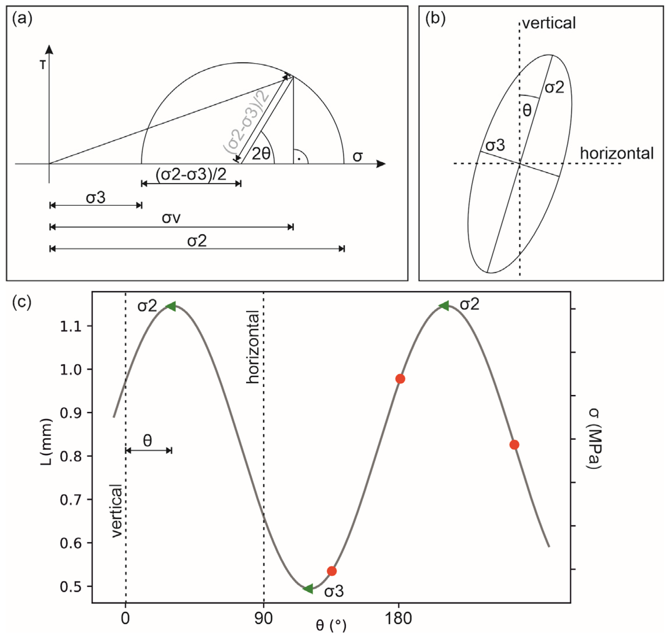
Let us assume that neither the least principal nor the intermediate principal stress is oriented vertically and that the intermediate principal stress is close to the vertical orientation. To take the offset angle θ between the vertical axis and σ₂ into account it has to be noted that the vertical stress (as it is not one of the principal stresses) contains a shear component (Figure 1).

Using the Mohr circle we can write the expression

$${\sigma }_v={\displaystyle \frac{{\sigma }_2+{\sigma }_3}{2}}+{\displaystyle \frac{{\sigma }_2-{\sigma }_3}{2}}cos 2\theta$$

(9)

for the vertical stress. In order to rewrite this expression in terms of σ₃ we can write Equation (9) as

$$0.5{\sigma }_3+0.5{\sigma }_3\cos 2\theta ={\sigma }_v-0.5{\sigma }_2+0.5{\sigma }_2\cos 2\theta$$

(10)

which allows to bring σ₃ to one side of the equation leading to

$${\sigma }_3={\displaystyle \frac{{\sigma }_v-0.5{\sigma }_2-0.5{\sigma }_{2}cos 2\theta }{0.5-0.5cos 2\theta }}$$

(11)

We now follow the derivation of Ebner et al. (2010) [25] with the angle correction which is detailed in Appendix A and arrive at an expression for ${\sigma }_1$ that includes the tilt angle $\theta$

$$\begin{array}{c}{\sigma }_1=-0.5 {\displaystyle \frac{{\sigma }_v\left(\left(\frac{1}{b}\frac{L_{min}}{L_{max}}+c\right)\left(1-\frac{a}{b}+\frac{a}{b}\frac{L_{min}}{L_{max}}\right)-\left(1+\frac{a}{b}-\frac{a}{b}\frac{L_{min}}{L_{max}}+d\right)\frac{1}{b}\frac{L_{min}}{L_{max}}\right)}{\left(1+\frac{a}{b}-\frac{a}{b}\frac{L_{min}}{L_{max}}+d\right)\left(1-\frac{a}{b}+\frac{a}{b}\frac{L_{min}}{L_{max}}\right)}}\\ \pm \sqrt{\begin{array}{c}0.25{\left({\displaystyle \frac{{\sigma }_v\left(\left(\frac{1}{b}\frac{L_{min}}{L_{max}}+c\right)\left(1-\frac{a}{b}+\frac{a}{b}\frac{L_{min}}{L_{max}}\right)-\left(1+\frac{a}{b}-\frac{a}{b}\frac{L_{min}}{L_{max}}+d\right)\frac{1}{b}\frac{L_{min}}{L_{max}}\right)}{\left(1+\frac{a}{b}-\frac{a}{b}\frac{L_{min}}{L_{max}}+d\right)\left(1-\frac{a}{b}+\frac{a}{b}\frac{L_{min}}{L_{max}}\right)}}\right)}^2\\ -\left({\displaystyle \frac{-{\sigma }_v^2\left(\frac{1}{b}\frac{L_{min}}{L_{max}}+c\right)\frac{1}{b}\frac{L_{min}}{L_{max}}-3\frac{e}{L_{max}}}{\left(1+\frac{a}{b}-\frac{a}{b}\frac{L_{min}}{L_{max}}+d\right)\left(1-\frac{a}{b}+\frac{a}{b}\frac{L_{min}}{L_{max}}\right)}}\right)\end{array}}\end{array}$$

(12)

with

$$a=0.5-0.5cos2\theta$$

(13)

$$b=a+0.5{\displaystyle \frac{L_{min}}{L_{max}}}-0.5{\displaystyle \frac{L_{min}}{L_{max}}} cos2\theta$$

(14)

$$c={\displaystyle \frac{1}{a}}-{\displaystyle \frac{1}{2ab}}{\displaystyle \frac{L_{min}}{L_{max}}}+{\displaystyle \frac{1}{2ab}}{\displaystyle \frac{L_{min}}{L_{max}}}cos2\theta$$

(15)

$$d={\displaystyle \frac{1}{2b}}{\displaystyle \frac{L_{min}}{L_{max}}}-{\displaystyle \frac{1}{2b}}+{\displaystyle \frac{1}{2b}}cos2\theta -{\displaystyle \frac{1}{2b}}{\displaystyle \frac{L_{min}}{L_{max}}}cos2\theta$$

(16)

$$e={\displaystyle \frac{\gamma }{\beta }}E$$

(17)

Equation (12) has two solutions, where most of the time one is either not solvable or not reasonable (i.e., negative values for σ₁).

The other two principal stresses can then be determined as follows (see Equation (A15) Appendix A)

$${\sigma }_3={c\sigma }_v+{d\sigma }_1$$

and (see Equation (A8) Appendix A)

$${\sigma }_2={{\displaystyle \frac{a}{b}}\sigma }_1-{{\displaystyle \frac{a}{b}}\sigma }_1{\displaystyle \frac{L_{min}}{L_{max}}}+{\displaystyle \frac{1}{b}}{\displaystyle \frac{L_{min}}{L_{max}}}{\sigma }_v$$

It should be noted that this derivation does not assume a tilt angle; the tilt angle can be directly derived when the cross-overs are determined. However, the value of the vertical stress is still needed (=depth).

2.2. Crossover Changes over Scales

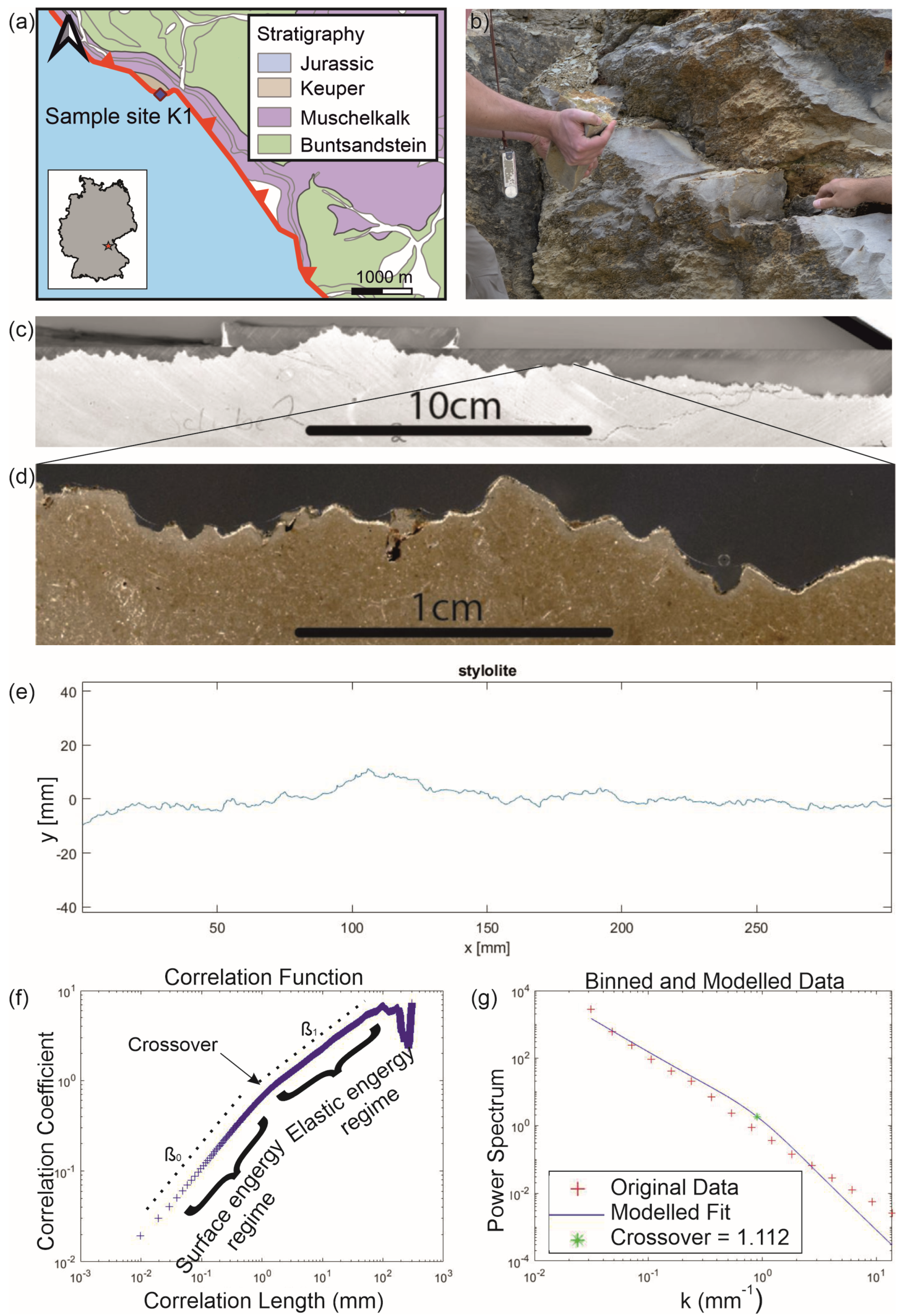
We test the processes and accuracy of the method with sample K1, which is taken from an outcrop consisting of Jurassic limestone in SE Germany (Figure 2a). The tectonic stylolites are associated with a SW-NE-directed tectonic inversion in the Cretaceous Period. This sample was analyzed by Koehn et al. (2022) [22] with special emphasis on dynamic scaling laws. The sample showed a strong and unambiguous signal, so it is ideal to be cut into smaller parts in order to evaluate the consistency of the crossover results. Figure 2 shows the complete process from sampling (Figure 2b), scanning the cut plane in high resolution (Figure 2c,d), digitizing the line drawing (Figure 2e) all the way to the analysis of the signal in MATLAB© (R2026a). There are a variety of methods to determine the crossover of a distinct stylolite, typically using either a Fourier Transformation, Wavelet Analysis, the correlation function or a Root Mean Square (RMS) analysis. In all cases the amplitude of the stylolite is observed on different lengths, expressing how the amplitude-wavelength relation changes over scales. To perform the Fourier Transformation leading to the power spectrum and to calculate the correlation function, a MATLAB© code written by Ebner et al. (2009) [23] was used. Examples for both are given in Figure 2f and g, respectively.

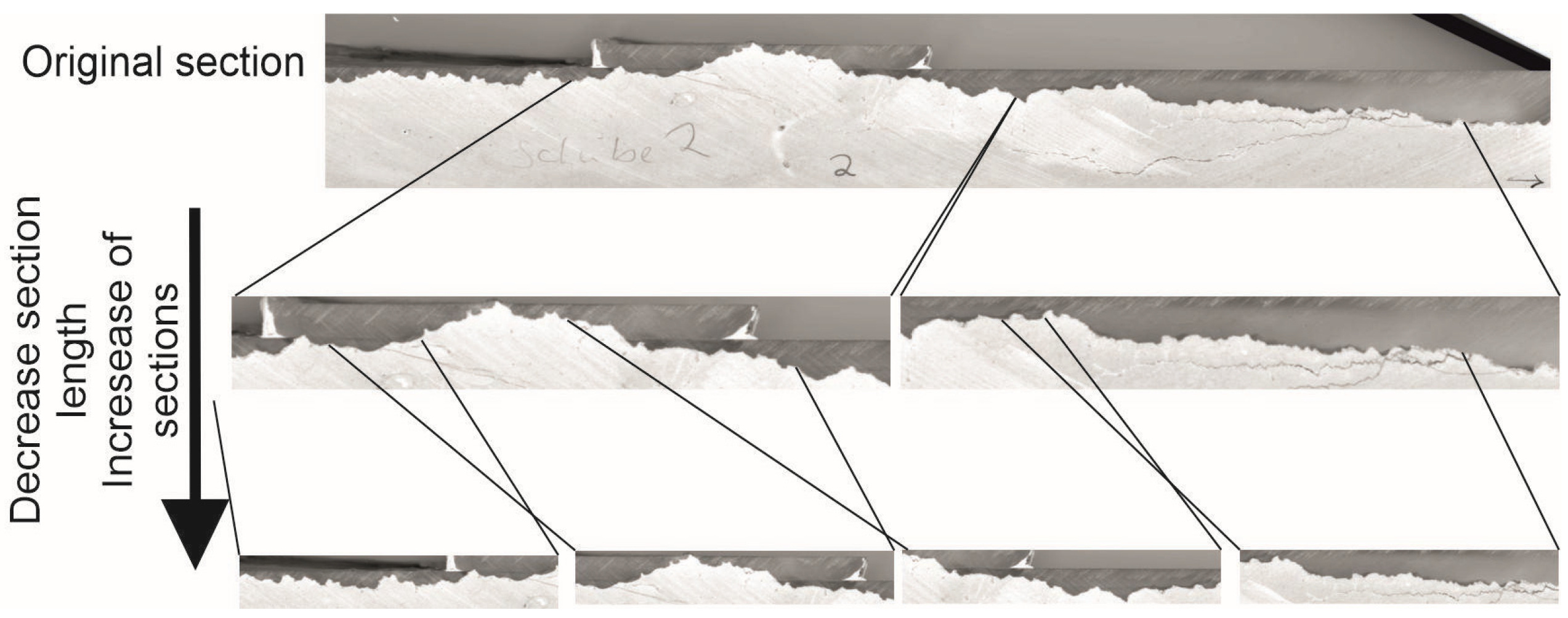
In the study of Koehn et al. (2022) [22] the authors proposed a crossover length L of about 1.4 mm. To scrutinize this value, the sample with an overall length of about 30 cm is split into smaller parts of 15, 10, 7.5, 5, 2.5 and 1.5 cm in length. Because of zooming into the sample we can increase the number of sections and thus the number of crossovers that can be extracted from one sample (Figure 3). For every section the correlation function was modeled and the crossover was determined. In addition, mean correlation functions of samples with the same size can be constructed and the crossover can be determined from the mean correlation function.

The accuracy of L is tested for all the mentioned correlation functions. In order to achieve this, two lines are fitted to the plot of the correlation function, one representing the slope (~0.7) on the small scale and one representing the slope (~0.5) on the large scale. For the estimation of the accuracy of the crossover, a variation in picking methods was used: (a) the intersection of the two slopes, (b) lower deviation of slope from data points and (c) upper deviation of slope from data points. Thus, the accuracy with respect to the section size can be compared. The correlation functions were weighted in terms of their quality from 1 (good) to 4 (no results). For statistical comparison we formed the mean of the picked crossovers. This allows us to calculate the standard deviation as well as the relative deviation. The process was performed for all crossovers weighted with quality 1 and 2 (Q2+) and for comparison for all with a quality of up to 3 (Q3+). The quality ranking takes the range between the upper and lower deviation from the slopes into account, as well as the deviation of the picked crossover from the intersection of the slopes and the deviation of the slopes from the ideal values of about 0.7 and 0.5. Correlation functions with weights of quality 4 were not taken into account for statistical interpretation. The results are presented in the Section 3.

2.3. Tectonic Stress Tensors for Different Samples

For the outcrop in Kirchleus (Figure 2a) we sampled eight different tectonic stylolites. For every sample the complete stress tensor is modeled. All samples were cut in three directions, horizontally (90°), vertically (0°) and diagonally (45°), with the exception of sample 8_2, which was cut at 20°, 70° and 45° (

Table 1. List of all samples with the orientation of the stylolite plane (Azimuth/Dip-direction) and the three directions of the cuts, relative to the vertical axis and perpendicular to the stylolite plane.

Sample	Orientation Stylolite Plane	Cut 1 (°)	Cut 2 (°)	Cut 3 (°)
K2	207/81	90	45	0
8_1_har	214/82	90	45	0
8_1_unhar	214/82	90	45	0
8_2	210/86	70	45	20
11_1	217/75	90	45	0
11_4_1	204/80	90	45	0
11_4_2	204/80	90	45	0
11_6	022/80	90	45	0

). For each sample we modeled as many crossovers as possible and weighted their quality from 1 (good) to 3 (unclear). We collected the lower and upper boundaries, where the data leave the mean slope as discussed in Section 2.2. Furthermore, we collected the point where the two slopes intersect and finally, we picked the crossover manually. For all of these types of crossovers from one sample we calculated the mean, standard deviation and median. As far as enough data was available, we used crossovers with quality 1 and 2 only. Using the mean of the picked crossovers as well as the upper boundary of each crossover and the respective standard deviation we created a range of crossovers for each sample. The stress tensor is then modeled for all respective combinations within these ranges, based on Equation (12). For all samples we used a Young’s modulus of E = 73 GPa [26] and a depth of 943 m [27], a Poisson Ratio of 0.258 and an interfacial free energy of 0.27 Jm⁻².

3. Results

3.1. Effects of Non-Vertical Principal Stresses on SRIT

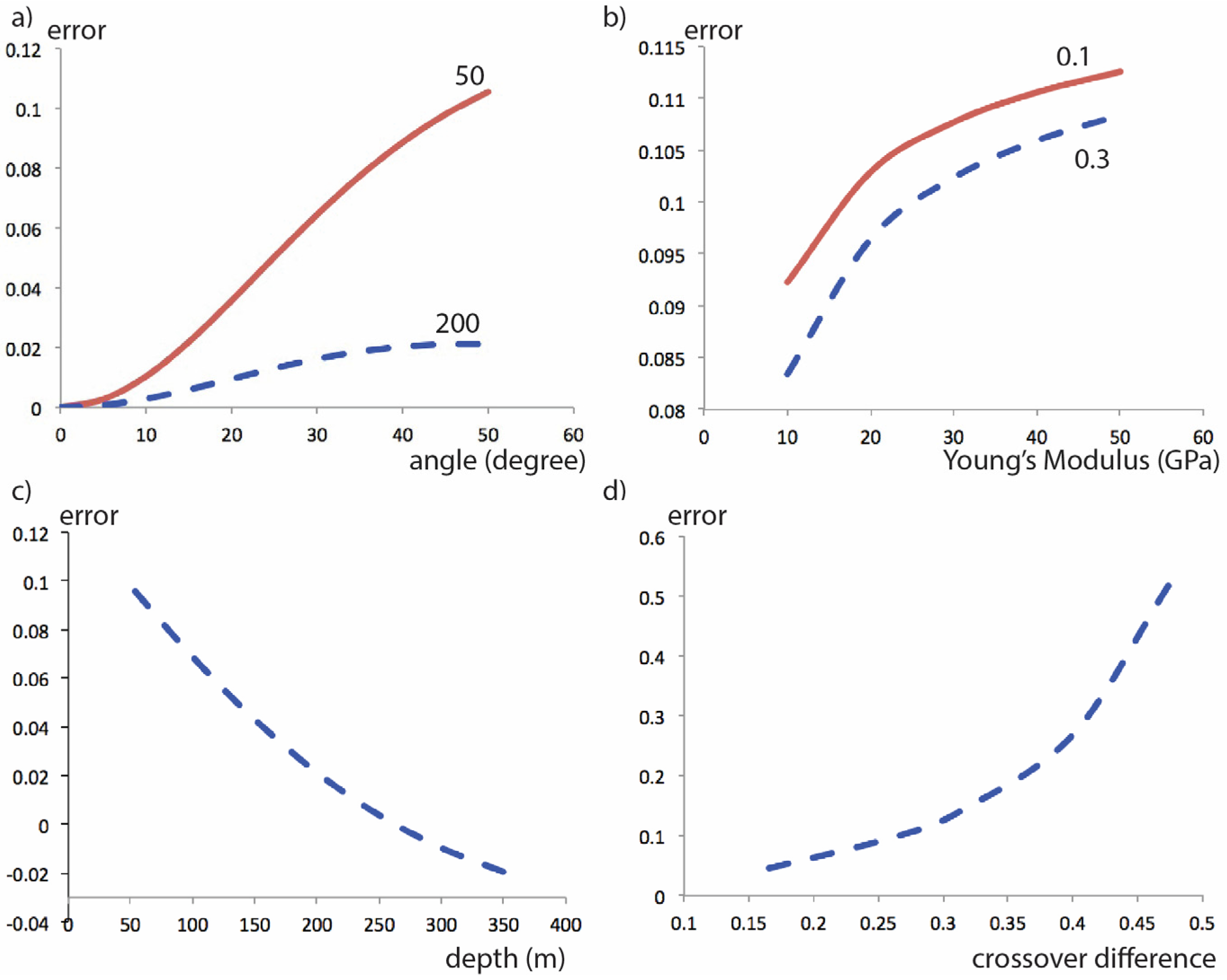
In this section we present a sensitivity analysis on the effects of non-vertically oriented principal stresses as well as several other input parameters of SRIT using Equation (12). Depending on the input parameters including the deviation from the vertical, the Young’s modulus, the Poisson ratio, the assumed vertical depth and the crossover ratio the error increases up to 50% in the extreme case. This is shown in Figure 4 with a typical stylolite from the outcrop in Kirchleus and a variation in the input parameters. Figure 4a shows that the effect of the error increases with the tilt of the principal stress relative to the vertical. This effect is increased by a decrease in the stylolite growth depth bringing the error from a maximum of 2% at a depth of 200 m all the way to a maximum of more than 10% at an assumed depth of 50 m. The Poisson ratio does not have a major effect on the error (Figure 4b) increasing it only by 1%. Young’s modulus however has a larger effect especially within the lower values with an overall increase in the error of 3% max. The burial depth or depth where the stylolite grew has an effect of up to 10% on the error with the largest deviations at shallow depth (Figure 4c).

The most important factor is the anisotropy of the in-plane stress, which relates to the (L_max − L_min)/L_max values in the plot (Figure 4d). The more anisotropic the in-plane stress and thus the difference between the two crossovers, the higher the effect of a tilted stress tensor with an error of up to 50% if the tilt angle is at a maximum. If the two crossovers are very similar, then the stress ellipse is close to a circle and the orientation of the in-plane stresses has no significant effect. However, if the in-plane stresses are very different (high anisotropy), then the angle of the principal stress relative to the horizontal axis will have a significant effect and the additional component in Equation (12) relative to the original equation [25] becomes important.

3.2. Accuracy of the Correlation Function in One Single Sample

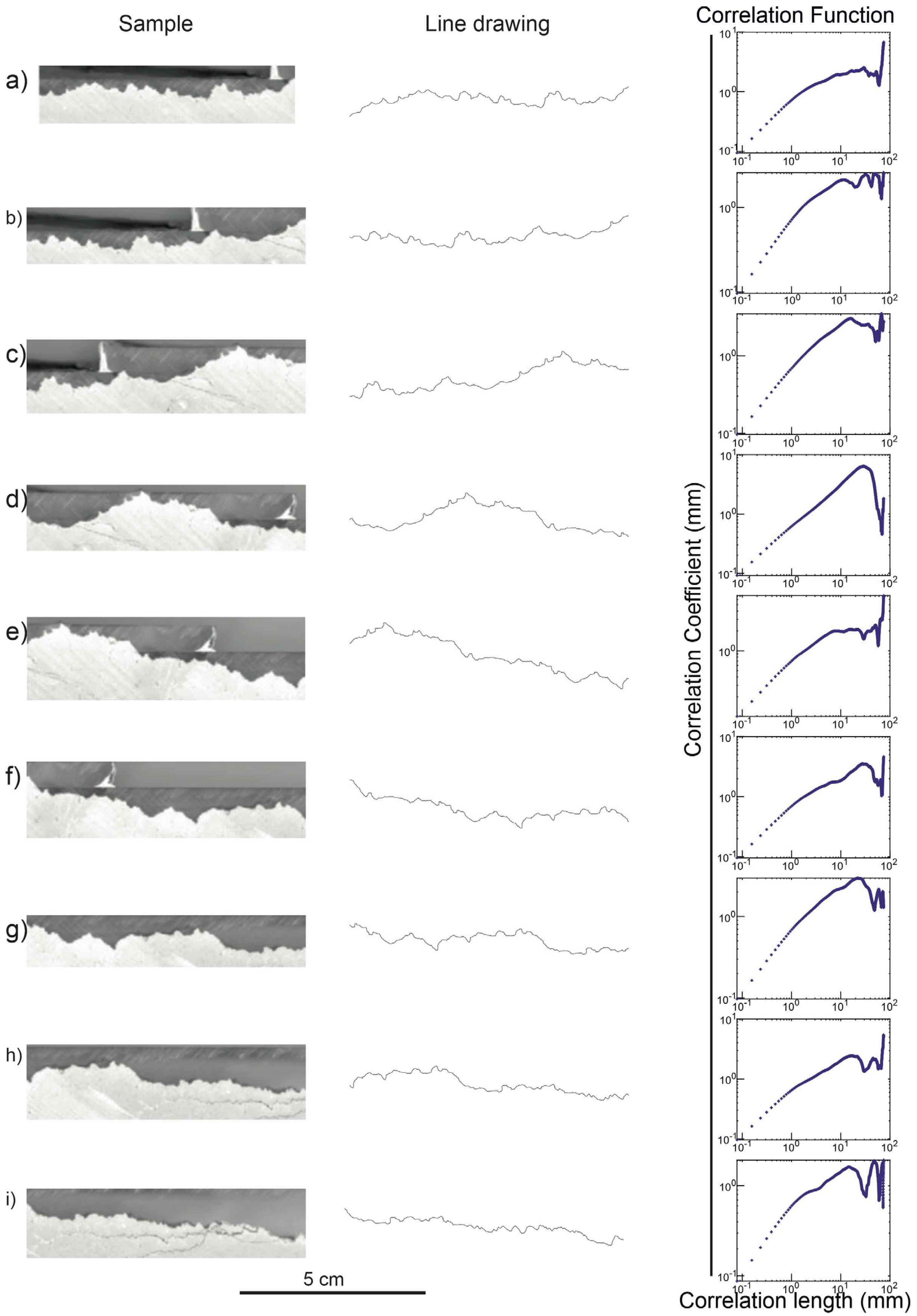
In this section we discuss how the correlation function changes within one sample of the same stylolite when different scans are taken and when a large scan line is divided into smaller sections. We also show how averaging over several sections changes the signal. Overall the 30 cm long original stylolite was cut into segments with lengths of 15, 10, 7.5, 5, 2.5 and 1.5 cm. One has to note that the accuracy of the determination of the crossover length does depend on the length-scale where the crossover is localized (typically mm to sub-mm and in this case at around 1.4 mm [22]), even though 10 cm long sections are thought to be ideal. The compilations of 10 cm segments in Figure 5, however, show that even on the 10 cm scale, shorter sections of the same stylolite show quite a variability. Here nine 10 cm long sections were taken from the original 30 cm long stylolite, so the sections overlap quite a bit. Irrespective of the overlap of the sections, the correlation functions on the right-hand side of Figure 5 show a high variability. On the smaller scale the signals are all still very similar with an almost identical slope for the surface energy-dominated regime. However, the switch to the second regime and thus the crossover varies for the different sections, as well as the slope in the elastic energy-dominated regime. At least sections c and d in Figure 5 show no clear crossover. Towards the largest scale of the correlation function the signal depends on the large-scale wavelength of the actual stylolite.

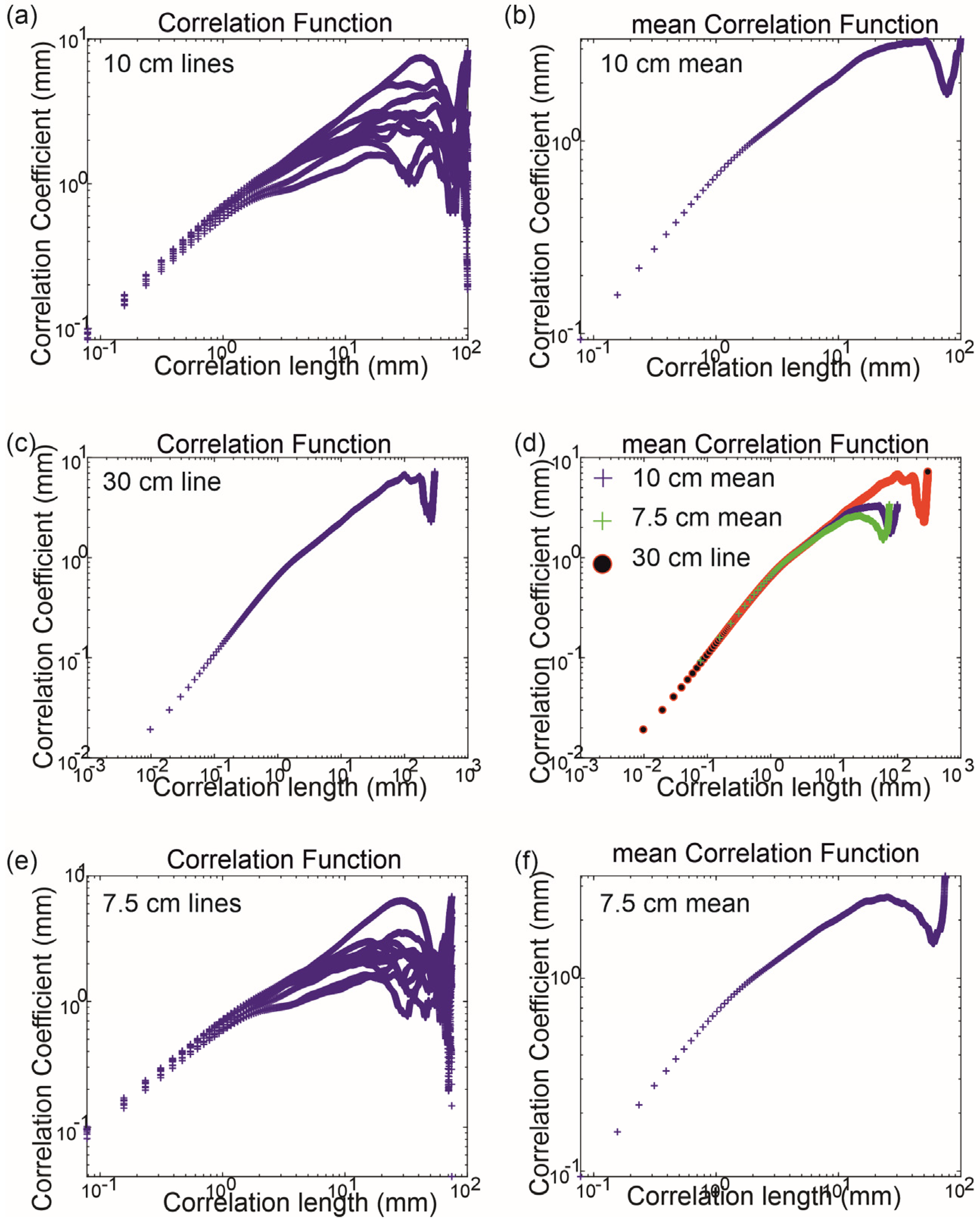
If a mean correlation function is undertaken, the results show less noise compared to the single sections (Figure 6). Figure 6b shows an average of the 10 cm long sections that are illustrated in Figure 6a. Once all sections are averaged, two well-defined slopes can be identified with a clear crossover. The resulting crossover length of the averaged 10 cm long sections coincides with the crossover produced by the 30 cm long stylolite as well as with the mean of the 7.5 cm segments (Figure 6d).

Generally we can observe that the shorter the section, the fewer correlation functions show clear crossovers. As a result of this phenomenon the amount of cross-sections that give quality 1, 2 and 3 (Q3+) results is almost constant across scales (

Table 2. Mean, standard deviation, relative deviation and number of data (N) for the respective section length (middle column) for qualities Q2+ or higher (left) and Q3+ or higher (right).

Q2+ L Mean (mm)	Std (mm)	Rel. Deviation (%)	N	Length (cm)	Q3+ L Mean (mm)	Std (mm)	Rel. Deviation (%)	N
1.15	0.06	5	8	15	1.4	0.4	25	10
1.1	0.1	10.4	5	10	1.2	0.2	14	6
1.2	0.1	11.6	4	7.5	1.2	0.2	18	10
1.5	0.1	8	5	5	1.3	0.2	13	8
1.4	0.03	3	3	2.5	1.2	0.4	25	10
None	None	None	0	1.5	1.3	0.3	20	6
1.3	0.2	14	23	All	1.3	0.3	22	51

).

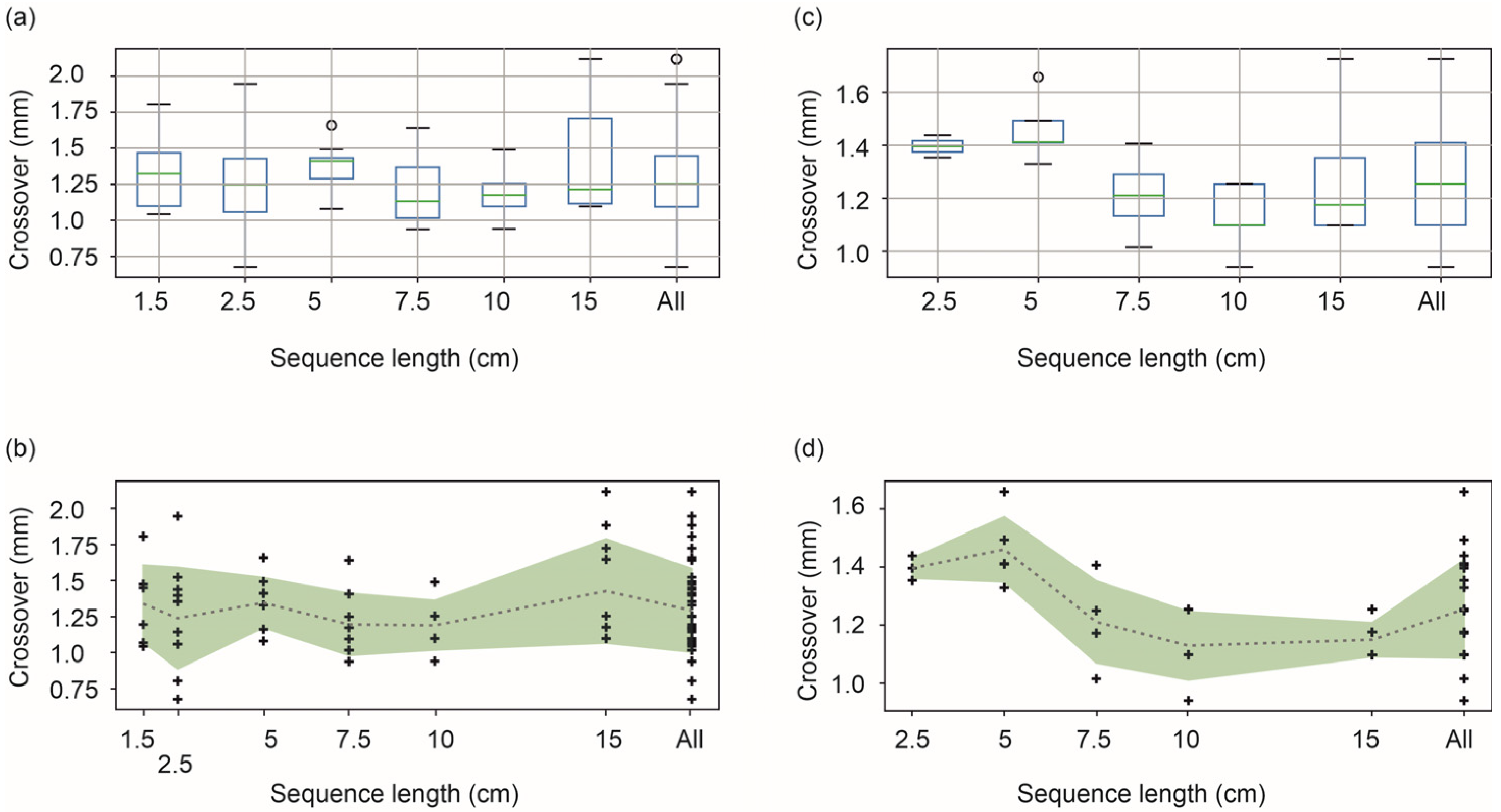
An overview of the SRIT inversion results for the different sizes is given in Figure 7 for quality 1, 2 and 3 (Q3+, Figure 7a,b) and only quality 1 and 2 (Q2+, Figure 7c,d). The picked crossover for the entire sample length of 30 cm lies in a range between 1.2 and 1.6 mm, due to the deviation of the data from lines with the ideal slopes of 0.7 and 0.5. For Q2+ the mean for the 15 cm sections lies at 1.15 ± 0.06 mm. For the section with a length of 10 cm the L_mean lies at 1.1 ± 0.1 mm. The mean of 7.5 cm section length is 1.2 ± 0.1 mm, for 5 cm section length 1.5 ± 0.1 mm and for 2.5 cm section length 1.40 ± 0.03 mm. However, no group of sections provides 10 or more data points with a quality of 2 or better. The 1.5 cm section length has no data weighted with quality 1 or 2. Calculating the mean and standard deviation of all Q2+ crossovers together (N = 23) we receive a mean of 1.3 ± 0.2 mm, which is a relative deviation of 14%.

For the quality group Q3+ with the lengths of 15 cm, 7.5 cm and 2.5 cm up to 10 sections are taken into account (Table 2). Altogether, 51 correlation functions belong to group Q3+. The section with the length of 15 cm gives a mean of 1.4 ± 0.4 mm, sections with the length of 10 cm give 1.2 ± 0.2 mm, sections with the length of 7.5 cm result in a mean crossover of 1.2 ± 0.2 mm, sections of 5 cm length give a mean of 1.2 ± 0.4 mm, the sections of 2.5 cm length lead to a mean L of 1.2 ± 0.4 mm and the smallest sections of 1.5 cm result in a mean of about 1.3 ± 0.3 mm. Taking all of these crossovers together (N = 51) the mean crossover is 1.3 ± 0.3 mm, which is a relative deviation of 22%. All resulting mean L-values are in the range of 1.2 to 1.5 mm with a maximum standard deviation of 0.4 mm and a relative deviation of 25%. Thus, the crossover of 1.4 mm picked from the longest stylolite section is within the range of the more detailed analysis. Assuming this would be the crossover of a stylolite with isotropic roughness (i.e., sedimentary stylolite) this would lead to a deviation of about 10% in the stress magnitude acting on the stylolite interface during growth, which is within the range of the normal error for SRIT.

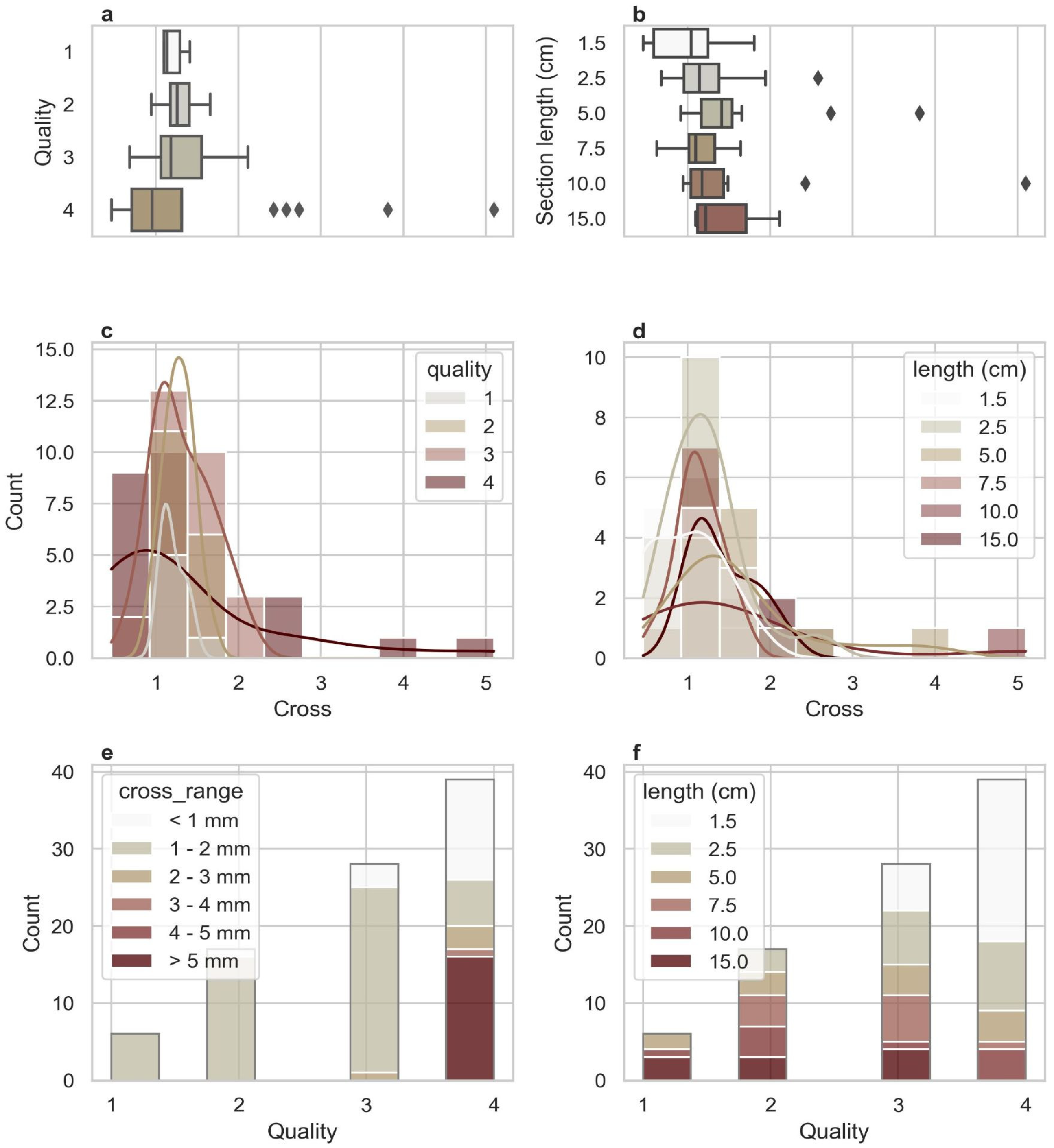
Figure 8 shows details of qualities and also the picked crossovers for the sections of different lengths. Quality 4 clearly contains a range of unrealistically high crossovers (Figure 8a) indicating that quality 4 should not be included in the analysis. A section length of 1.5 cm significantly deviates from crossovers given by the other length segments (Figure 8b) and one can also observe that this scale has the most sections with low quality (Figure 8f). However, one can also see that almost all sections contain outliers that give unrealistic crossover lengths (Figure 8b). The spread of crossover results obtained from quality 4 crossovers can also be seen in Figure 8c as well as Figure 8e illustrating that within this quality most crossovers are too large or too small. The picture changes significantly for quality 3, 2 and 1 crossovers. These are within a reasonable range and give good results. In accordance with the data from Table 2, Figure 8f shows that the amount of quality 2 crossovers that give a reasonable result spreads evenly across lengths 2.5, 5, 7.5, 10 and 15 cm. However, one has to keep in mind that a lot more sections were used for the length of 2.5 cm than for the length of 15 cm.

3.3. Consistency of the Crossover Length Within One Outcrop

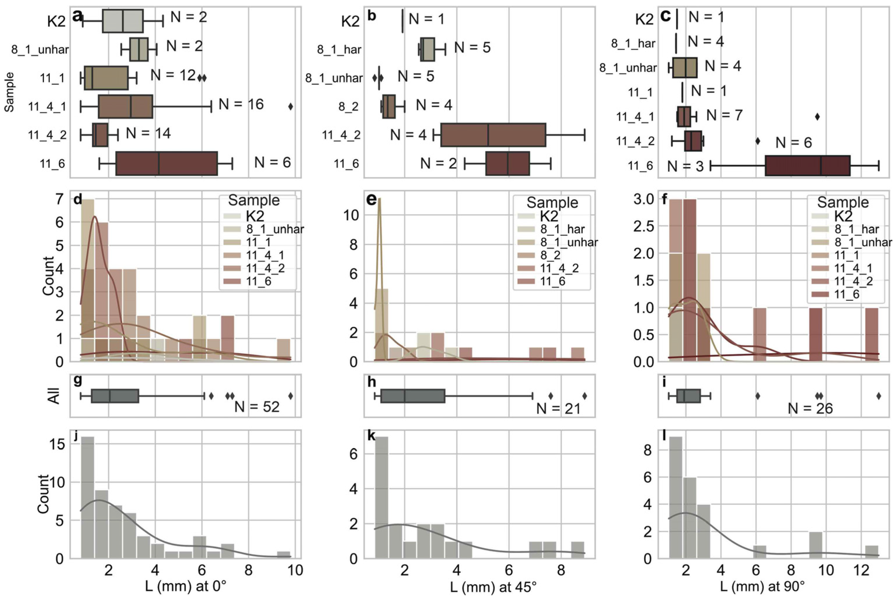
To evaluate the consistency of stylolite roughness inversion within one outcrop, crossovers from all eight samples from the respective outcrop are compared. In Figure 9 all crossovers are shown, regardless of their quality. Note that the columns in Figure 9 represent the different orientations where the crossover was measured, so not all samples can be shown, since not all of them were cut in the same orientation (Table 1). For the final calculation of the stress tensor, only Q3+ is used. The crossovers of the vertical axis (0°) have an Interquartile Range (IQR) of about 0.5 to 4 mm. Sample 11_6 is an exception with an IQR ranging from 2 to more than 6 mm. The crossovers at an orientation of 45°, middle column in Figure 9, show a large distribution, ranging from 0.7 to 11 mm, with a small peak at 2 mm. In the horizontal orientation the range of the crossovers is very narrow, except for sample 11_6. Excluding sample 11_6, all IQRs are in the range of about 1 to 3 mm. Comparing the histograms from the separated and the summed data sets, the peaks of the crossover are shifted only slightly.

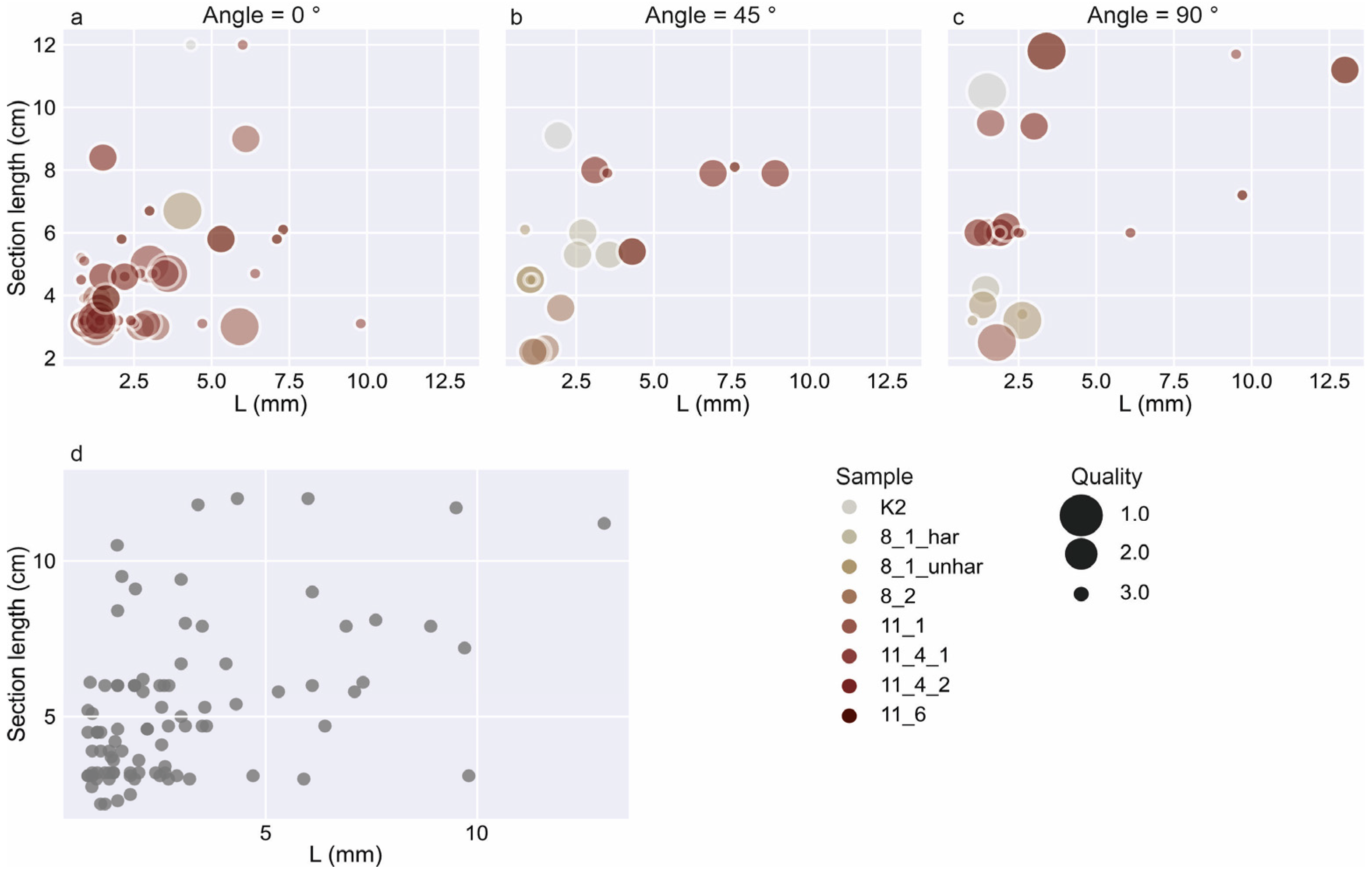
In the following section only values falling in the IQR of the corresponding box plot diagrams are described. Outliers are neglected. The highest amount of data is provided for the vertical direction (N = 51). The range of resulting L-values is similar for all groups of quality. In contrast, looking at the data separated with respect to the section length, the L-values can be split into three groups of ranges. The small section (2–4 cm) leads to an L-range of about 1–2 mm, sections with a length of 4–6 cm lead to an L-range of about 2–3.5 mm, and finally, sections longer than 6 cm provide an L-range of about 3.5–6 mm (Figure 10). For the cut direction with a tilt of 45° no crossovers are weighted with a quality of 1. This cut direction contains only 19 data points. The L-values do not correlate with the data quality, similar to the data in the vertical direction. Another similarity is that the length of the section allows us to cluster the resulting L-values. Sections with a length of 2–4 cm have the tightest L-range of about 1–1.5 mm. Sections with a length of 4–6 cm lead to small L-values of about 1 mm, but range up to 3 mm. Sections longer than 6 cm lead to an L-range of about 3–7 mm. However, the numerical peak L-value is at about 1 mm, while higher values are represented only by single data points. The horizontal cut direction with N = 23 data points gives a different picture. While crossovers weighted with quality 1 and 2 are at the same level of about 1.5–2.5 mm, the group weighted with quality 3 has a much higher range with L-values of up to 6 mm. Separating the crossovers with respect to section length, sections with a length smaller than 8 cm lead to the mean L-range of 1.5 to 2.5 mm. Sections longer than 8 cm produce an IQR up to 8 mm. In all three directions we cannot observe a correlation between data quality and section length (Figure 10). However, there is a tendency for a correlation between crossover length and section length, at least for the vertical and tilted sections, whereas the horizontal sections do not show this correlation.

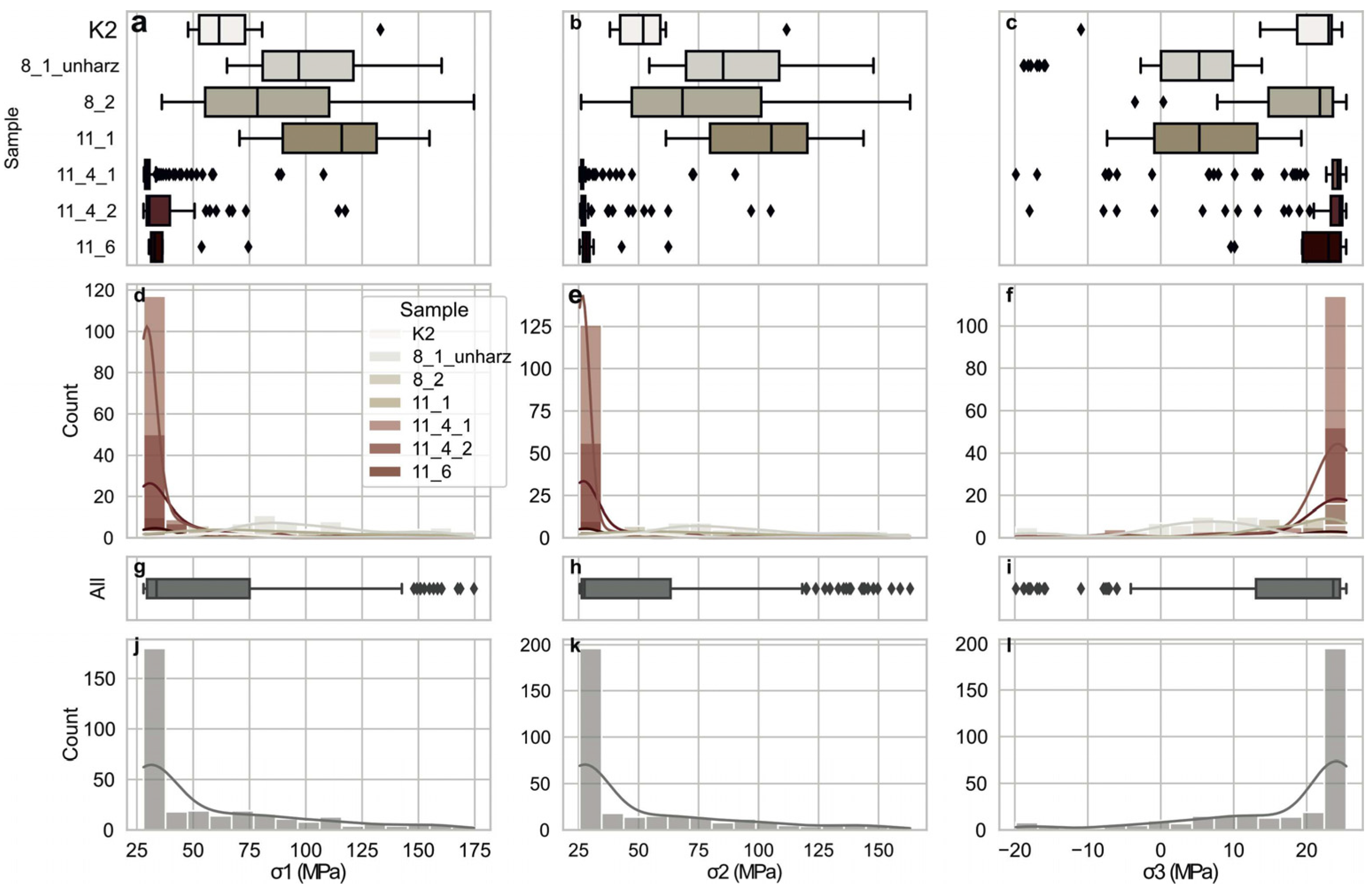
The calculated mean and median principal stresses for all samples are listed in

Table 3. Calculated principal stresses (σ_1–3) with absolute and relative standard deviation. N is the number of successful model runs.

Sample	σ1 ± Std (MPa) [Std%]	Median (MPa)	σ2 ± Std (MPa) [Std%]	Median (MPa)	σ3 ± Std (MPa) [Std%]	Median (MPa)	N
K2	68 ± 23 [34%]	61	56 ± 20 [35%]	52	18 ± 10 [53%]	23	11
8_1_unhar	110 ± 32 [30%]	99	96 ± 32 [33%]	87	3 ± 10 [375%]	5	56
8_2	70 ± 25 [35%]	66	63 ± 24 [38%]	60	6 ± 12 [160%]	8	143
11_1	112 ± 29 [26%]	116	102 ± 28 [28%]	105	6 ± 9 [156%]	5	7
11_4_1	33 ± 11 [34%]	30	28 ± 8 [29%]	26	21 ± 8 [38%]	24	135
11_4_2	38 ± 17 [45%]	30	32 ± 14 [45%]	27	21 ± 8 [40%]	25	68
11_6	38 ± 12 [33%]	33	32 ± 10 [32%]	28	21 ± 5 [25%]	23	12
Mean	56 ± 33 [59%]	33	50 ± 30 [60%]	28	14 ± 12 [86%]	23	437

, including standard deviation and relative deviation. The number of data points (last column) depends on the number of reasonable results. We neglected combinations of crossovers that result in a stress ratio φ > 1.

In addition, we neglected combinations leading to σ₃ < −20 MPa. Especially for small σ₃-values the relative deviation is high (up to 375%), while the absolute standard deviation is smaller than for σ₁ and σ₂. This is due to the mean values of σ₃ being close to 0 MPa. For samples 8_1_unhar and 8_2, the standard deviation of σ₃ leads to a range from negative to positive values and thus the potential of tensional stress.

Strengthened by the plots in Figure 11 and Figure 12, the data show that we can separate the samples into two groups. Group (1) consists of samples 11_1, 11_4_1, 11_4_2 and 11_6. The IQR of these samples is rather tight for all principal stresses. As the magnitudes of σ₁, σ₂ and σ₃ are relatively high, the resulting stress ratio φ is rather small, ranging from about 0.35 to 0.55. Group (2) consists of samples 8_1_unhar, 8_2 and K2. IQRs of all samples have a much wider range than those of group (1), so that σ1 reaches from 50 to 130 MPa. σ₃ of sample K2 is closer to the range of group (1). In general, σ₃ values in group (2) are in the range of about 3–18 MPa. The higher difference in σ₁ and σ₂ towards σ₃ compared to group (1) results in a higher range of the stress ratio φ from 0.65 to 0.95. However, the two groups show clearly separated distributions. Whether or not the two groups are geologically relevant is debatable and is discussed further in the Section 4.

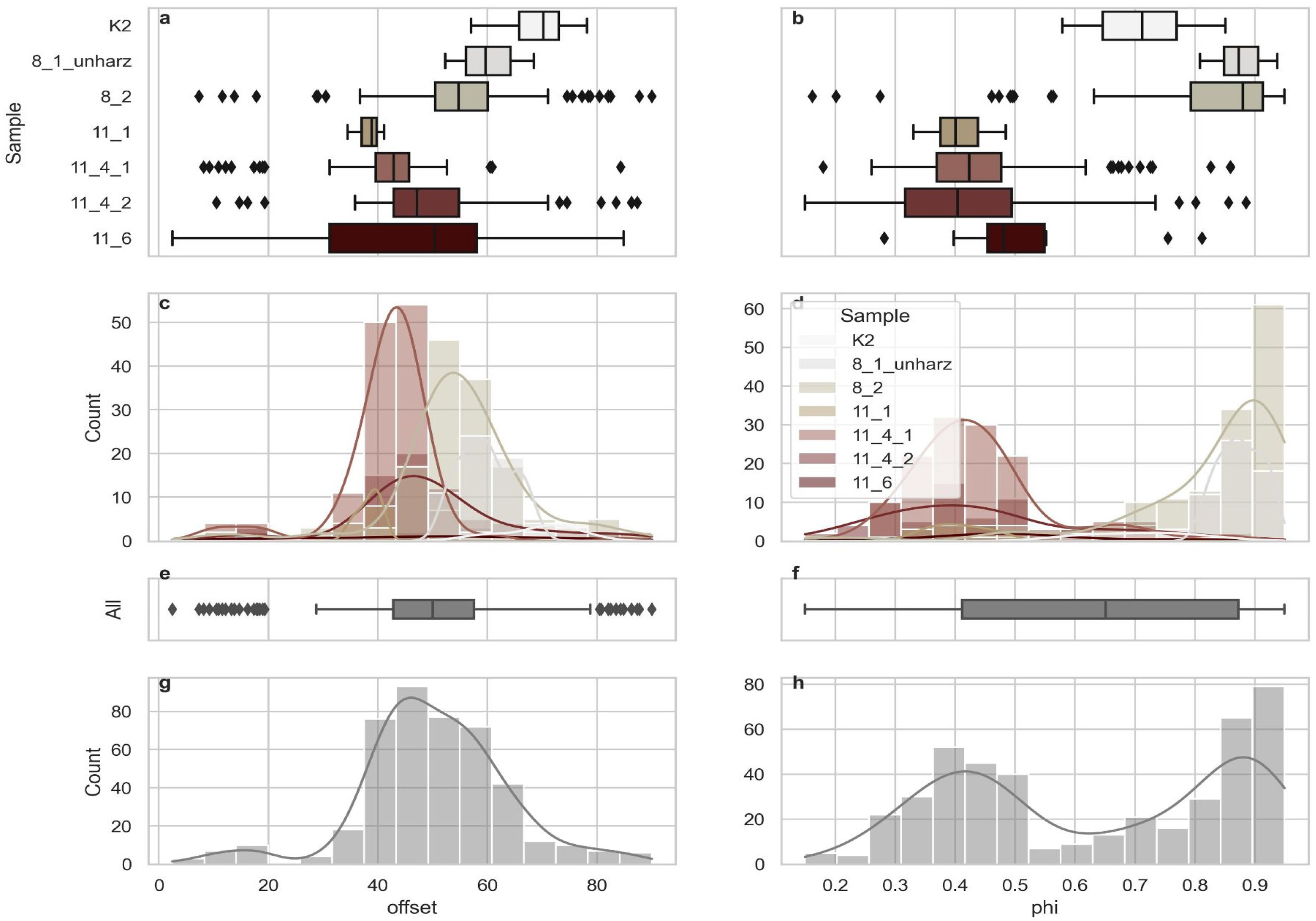
The resulting offset angles of the principal stresses in the stylolite plane relative to the horizontal are visualized in Figure 12, showing box plot diagrams for all samples in (a) and a histogram in (c). The median values of all samples are in the range of 40 and 70°. The IQR and histogram show the distribution of all samples in sum. The median is at 50°, while the peak of the histogram is at 45°. Sample 11_6 has a high IQR of about 35 to 60°. Sample 11_4_2 has values plotting below 20°; however, the IQR is stabilized in the range of about 45 to 55°. According to the two groups mentioned before, group (2) IQRs are between 55 and 70°, while the IQR of group (1) is framed by the IQR of sample 11_6. The other three samples in this group have much tighter IQRs, together in the range of 35–55°. As the offset gives the angle between the vertical axis and the long axis of the in-plane stress ellipse, the offset correlates with the angle between the vertical axis and σ₂. In consequence, all samples are in the transition between strike-slip and thrust faulting regimes.

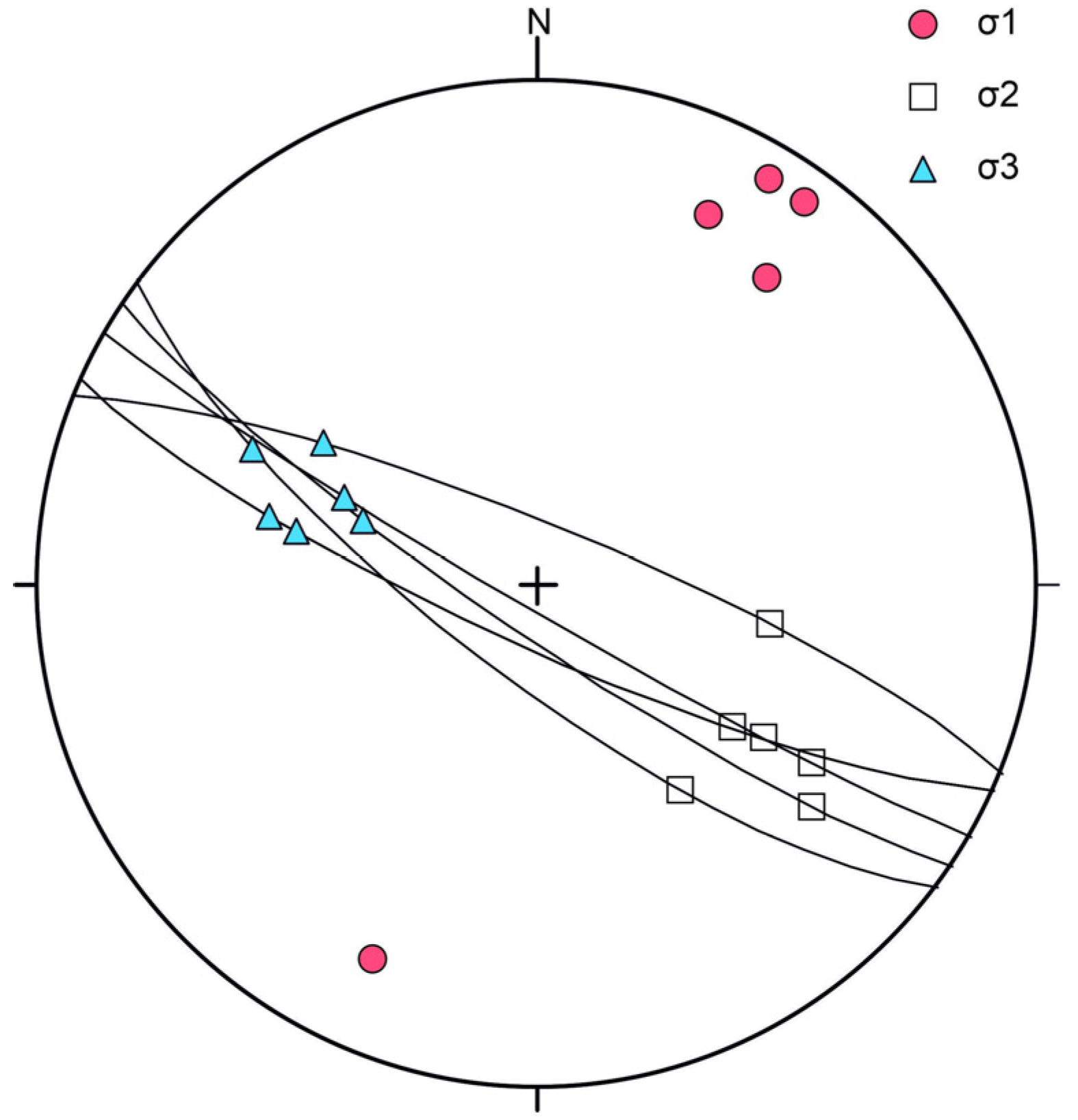
Figure 13 shows the stereographic projection of the main principal stresses of the stress tensors resulting from the orientation of the samples and the modeled offset angles of the in-plane stresses σ₂ and σ₃. In-plane stresses are transferred to the great circle of the stylolite plane. σ₁ and σ₂ show a strong proportional correlation. In contrast, the correlation between σ₁ and σ₃ is more diffuse. σ₃ tends to decrease with an increase in the highest principal stress. σ₁ and σ₂ show an exponential relation to φ. For σ₃ it is the other way around. An increase in σ₃ leads to an exponential decrease in φ. A similar behavior can be described for L_min. An increase in L_min leads to an exponential increase in σ₁ and σ₂, while σ₃ is decreasing exponentially. Figure 12 shows the correlation between the principal stresses and the calculated offset angle θ. High magnitudes of the medium and highest principal stresses coincide with offset angles of θ > 50°, whereas low magnitudes can lead to a high range of θ. For the high offset angles the smallest principal stress shows the corresponding minimum. Another minimum is at about 10°. The magnitudes of the stresses become stable with an L_min value of about 2 mm.

4. Discussion

4.1. Necessity of Angle Correction

Stress inversion of vertically oriented tectonic stylolites normally implies that one of the main principal stresses is vertical. In this contribution we showed that negligence of the shift in the stress ellipse can lead to a misfit of the calculated stresses of up to 50%. In addition, our results show that the effect of the shift strongly correlates with the magnitude of the respective variables. For samples at a larger depth the misfit is rather low (<1%), while a shallow depth produces the maximum calculated misfit. All the other parameters are highly sensitive as long as stresses are acting at a shallow depth. In this case a high anisotropy, higher Young’s modulus and lower Poisson ratio increase the calculated misfit.

However, this effect is an additional error to the error produced by uncertainty in the crossover length, the assumed depth and the rock physical parameters. Therefore, at shallow depth such angle correction is highly recommended to minimize the overall misfit. As the misfit decreases with depth, the need for correction decreases as well. In turn, as we are dealing with a wide range of uncertainties we highly recommend minimizing the additional uncertainty produced by modeling and thus, the angle correction presented here should always be applied.

4.2. Crossover Accuracy Through Sample-Scale

The analysis of the horizontal cut of sample K1 with its total length of 30 cm shows a high consistency of the received crossovers down to the section length of 2.5 cm (Figure 8b,d). The smallest section of 1.5 cm length has an increased IQR, while the mean L-value is still close to those of the longer sections. However, the quality of the signals varies independently of the section length (Table 2, Figure 8). With the exception of the smallest section of 1.5 cm length, all lengths provide signals with high quality (Q2+). The mean signal is visible in correlation functions of all qualities (Figure 8e). The mean crossovers of all sections (Q3+) are within the acceptable error of the original signal of the total sample. In addition, all scales provide sections that produce no signal.

In turn, we show that the assumed “true” crossover length is visible through all sample scales. At the same time, outliers exist across all scales as well. As shown in the left column of Figure 8 selecting the crossover by the quality of the signal only may be misleading, as signals weighted with quality 3 and 4 can give true L-values. Calculating the mean correlation function (Figure 6b,d) reduces the impact of the noise. This increases the statistical reliability of the result.

However, the question of the perfect sample length remains unanswered, except for the result that a 1.5 cm length is too small, due to the high amount of correlation functions with very low quality or no signal.

4.3. Accuracy Through Outcrop-Scale and Implications for Regional Geology

To evaluate how representative a single sample is for an entire outcrop we analyzed eight samples from the same outcrop. As shown in Figure 9, the crossovers scatter in a relatively wide range. The number of useful crossovers varies from sample to sample and depends on the orientation of the cut. Sample 11_6 provides only 6, 2 and 3 useful crossovers for the respective orientations. The corresponding IQR is much wider than for the other samples. This could be an indicator that such a sample should not be used for further models.

Altogether the samples show (sample 11_6 excluded) a high consistency in the horizontal orientation; the vertical and oblique orientations have wider IQRs.

The principal stresses for each sample are modeled based on a range of input crossovers. The width of the range (minimum to maximum value) depends on the standard deviation of the modeled crossovers and of the different methods (picked value plus lower and upper boundary, where the data leaves the ideal slopes) to gain the value from the correlation function. In turn, the deviation of the modeled stresses depends strongly on the width of the L-range. In the case of a high-quality correlation function, the two methods lead to similar results, while low-quality correlation functions provide more diversity. That means the higher the accuracy of the crossovers, the higher the accuracy of the stress magnitudes.

The standard deviation of the modeled principal stresses becomes quite high, while at the same time the IQR is small. Thus, the impact of outliers is quite high. Therefore, we propose that future SRITs use the IQR instead of the mean and standard deviation.

The modeled stresses show two groups. One with a stress ratio φ~0.4 and the other with φ~0.9. The same goes for the offset angle θ, where the first group has an offset of around 40°, while the second group peaks around 50°. However, the calculation of the second group is based on much less data than the first (Figure 9 and Figure 11). The question regarding the observation of these two groups is: are there two phases of stylolite growth or are the two phases only noise artifacts?

On the one hand the offset angle θ shows these two peaks; on the other hand all samples potentially grew in the same stress regime, with σ₁ in a NE-SW direction and tilted σ₂ and σ₃ with σ₂ being tilted by about 40° towards SE. Thus, no sample has a principal stress axis in the vertical orientation. There are a few possible scenarios proposed for such oriented stress fields: (a) the transition between thrust faulting and strike-slip regimes [27] and (b) the vicinity to the Eisfeld–Kulmbach Fault (Figure 2). Both scenarios could lead to a tilt of the stress tensor.

Two distinct clusters of stresses can be derived: one cluster shows applied stresses of σ₁~30 MPa, σ₂~28 MPa and σ₃~23 MPa and a second cluster shows applied stresses of σ₁~70 MPa, σ₂~60 MPa and σ₃~10 MPa. Both are realistic stress fields but we cannot rule out that they are derived as a function of uncertainty in the data. The data show tectonic stresses that were active during the Cretaceous inversion in central Europe in the footwall of the Eisfeld–Kulmbach reverse fault. Stress inversion data on the fault slip surface [27,28,29] indicates that the stress field switched from compressional to strike slip during the inversion [30,31,32]. This switch may be reflected in (a) the consistent tilt angle of principal stresses within the stylolite plane and (b) the two derived stress clusters. Stylolites record a time series and not a single event and can therefore contain overprinted stress fields.

The current stress field is oriented roughly perpendicular to the Cretaceous stylolites so that the main compressive stress is now oriented roughly parallel to the stylolite plane. Potentially that makes the Cretaceous stylolites prone to being reactivated as extensional cracks. This cannot be observed in the studied outcrop but in some other localities in Northern Bavaria [31,32]. Theoretically if the main compressive stress is oriented at an angle to the plane of the Cretaceous stylolites they could also be activated as faults or shear surfaces [33] but since they are very rough surfaces this is probably not the case.

4.4. Significance of the Results

The analysis shows that the method deals with a lot of uncertainties (i.e., depth and rock physical parameters during stylolite growth) and is only valid for stresses stored by pressure solution. In our case, where the samples are from the same outcrop, uncertainties in the rock physical parameters are assumed to be equal for all samples. However, we cannot say for sure that all samples grew at the same time and thus at the same depth. We assume that depth does not change significantly during the potential phases of stylolite growth. Therefore, in the frame of those uncertainties the crossovers are comparable and the relation L_min/L_max is valid. And thus, the orientation of the stress tensor is independent of the parameters assumed for the quantification. The validation of the modeled stress magnitude can be increased through more information regarding burial depth and the physical behavior of the rock and the interacting fluids.

5. Conclusions

In this contribution we derive a new equation for the tectonic stylolite stress inversion SRIT that corrects for tilted principal stresses in the stylolite plane. We show that in cases where the tilt is relatively strong the error in the derived stress values can increase to up to 50%, with 10% being a relatively common error. Therefore, we recommend the use of the correction.

Irrespective of the sample size, a single sample of a stylolite does not necessarily allow for a correct stress inversion. Therefore, we advise taking several profiles along a stylolite and averaging the resulting scaling functions to derive better results. With an average crossover of 1.3 mm in our sample the minimum sample size is 2.5 cm for the derivation of meaningful results. This implies that stylolite signals that are used for SRIT should be at least 20 times the crossover length. This of course imposes the problem that the crossover length is not known a priori.

The derived crossovers and thus the stress inversion show relatively large variations between samples in the outcrop. However, two distinct clusters of stresses can be derived but it is not clear whether or not these represent two real tectonic phases or not. However, the offset angle is consistently stored in multiple stylolites from one outcrop. Therefore, the assumption that one principal stress is always in the vertical axis does not seem to be valid at least for this outcrop.

References

1. Park, W.C.; Schot, E.H. Stylolites: Their Nature and Origin. J. Sediment. Petrol. 1968, 38, 175–191. [Google Scholar] [CrossRef] [Scilit]
2. Bruna, P.-O.; Lavenu, A.P.; Matonti, C.; Bertotti, G. Are stylolites fluid-flow efficient features? J. Struct. Geol. 2019, 125, 270–277. [Google Scholar] [CrossRef] [Scilit]
3. Elliott, S.J.; Forstner, S.R.; Wang, Q.; Corrêa, R.; Shakiba, M.; Fulcher, S.A.; Hebel, N.J.; Lee, B.T.; Tirmizi, S.T.; Hooker, J.N.; et al. Diagenesis is key to unlocking outcrop fracture data suitable for quantitative extrapolation to geothermal targets. Front. Earth Sci. 2025, 13, 1545052. [Google Scholar] [CrossRef] [Scilit]
4. Lacombe, O.; Beaudoin, N.E.; Hoareau, G.; Labeur, A.; Pecheyran, C.; Callot, J.-P. Dating folding beyond folding, from layer-parallel shortening to fold tightening, using mesostructures: Lessons from the Apennines, Pyrenees, and Rocky Mountains. Solid Earth 2021, 12, 2145–2157. [Google Scholar] [CrossRef] [Scilit]
5. Peacock, D.C.P.; Sanderson, D.J.; Leiss, B. Use of Analogue Exposures of Fractured Rock for Enhanced Geothermal Systems. Geosciences 2022, 12, 318. [Google Scholar] [CrossRef] [Scilit]
6. Sanderson, D.J.; Peacock, D.C.; Nixon, C.W. Fracture sets and sequencing. Earth-Sci. Rev. 2024, 257, 104888. [Google Scholar] [CrossRef] [Scilit]
7. Hupkes, J.; Bruna, P.O.; Bertotti, G.; Doesburg, M.; Moscariello, A. A fracture rarely comes alone: Associations of fractures and stylolites in analogue outcrops improve borehole image interpretations of fractured carbonate geothermal reservoirs. Solid Earth 2026, 17, 113–134. [Google Scholar] [CrossRef] [Scilit]
8. Gernlold, Z.; Gerdes, A.; Hezel, D.; Hohmeier, B.; Linckens, J.; Mertineit, M. Tectonic stylolites in anhydrite rock: Constraints on fluid-assisted deformation and isotopic ags of salt rocks (Gorleben salt dome Germany). Tectonophysics 2026, 933, 231250. [Google Scholar] [CrossRef] [Scilit]
9. Nitecki, M.H. Observations on Slickolites. J. Sediment. Res. 1962, 32, 435–439. [Google Scholar] [CrossRef] [Scilit]
10. Koehn, D.; Renard, F.; Toussaint, R.; Passchier, C.W. Growth of stylolite teeth patterns depending on normal stress and finite compaction. Earth Planet. Sci. Lett. 2007, 257, 582–595. [Google Scholar] [CrossRef] [Scilit]
11. Laronne Ben-Itzhak, L.; Aharonov, E.; Toussaint, R.; Sagy, A. Upper bound on stylolite roughness as indicator for amount of dissolution. Earth Planet. Sci. Lett. 2012, 337–338, 186–196. [Google Scholar] [CrossRef] [Scilit]
12. Renard, F.; Schmittbuhl, J.; Gratier, J.-P.; Meakin, P.; Merino, E. Three-dimensional roughness of stylolites in limestones. J. Geophys. Res. Solid Earth 2004, 109, B03209. [Google Scholar] [CrossRef] [Scilit]
13. Rustichelli, A.; Tondi, E.; Agosta, F.; Cilona, A.; Giorgioni, M. Development and distribution of bed-parallel compaction bands and pressure solution seams in carbonates (Bolognano Formation, Majella Mountain, Italy). J. Struct. Geol. 2012, 37, 181–199. [Google Scholar] [CrossRef] [Scilit]
14. Rustichelli, A.; Tondi, E.; Korneva, I.; Baud, P.; Vinciguerra, S.; Agosta, F.; Reuschlé, T. Bedding-parallel stylolites in shallow-water limestone successions of the Apulian Carbonate Platform (central-southern Italy). Ital. J. Geosci. 2015, 134, 513–534. [Google Scholar] [CrossRef] [Scilit]
15. Aharonov, E.; Katsman, R. Interaction between pressure solution and clays in stylolite development: Insights from modeling. Am. J. Sci. 2009, 309, 607–632. [Google Scholar] [CrossRef] [Scilit]
16. Harris, J. Fractal Architecture: Organic Design Philosophy in Theory and Practice; UNM Press: Albuquerque, NM, USA, 2012. [Google Scholar]
17. Mandelbrot, B.B. The Fractal Geometry of Nature; W. H. Freeman and Company: San Francisco, CA, USA, 1982. [Google Scholar]
18. Mandelbrot, B. How long is the coast of britain? Statistical self-similarity and fractional dimension. Science 1967, 156, 636–638. [Google Scholar] [CrossRef] [Scilit] [PubMed]
19. Mandelbrot, B.B. Getting snowflakes into shape. New Sci. 1978, 78, 1107. [Google Scholar]
20. Barabási, A.-L.; Standley, H. Fractal Concepts in Surface Growth; Cambridge University Press: Cambridge, UK, 1995. [Google Scholar]
21. Schmittbuhl, J.; Renard, F.; Gratier, J.P.; Toussaint, R. Roughness of stylolites: Implications of 3D high resolution topography measurements. Phys. Rev. Lett. 2004, 93, 238501. [Google Scholar] [CrossRef] [Scilit]
22. Koehn, D.; Köhler, S.; Toussaint, R.; Ghani, I.; Stollhofen, H. Scaling analysis, correlation length and compaction estimates of natural and simulated stylolites. J. Struct. Geol. 2022, 161, 104670. [Google Scholar] [CrossRef] [Scilit]
23. Ebner, M.; Koehn, D.; Toussaint, R.; Renard, F.; Schmittbuhl, J. Stress sensitivity of stylolite morphology. Earth Planet. Sci. Lett. 2009, 277, 394–398. [Google Scholar] [CrossRef] [Scilit]
24. Toussaint, R.; Aharonov, E.; Koehn, D.; Gratier, J.-P.; Ebner, M.; Baud, P.; Rolland, A.; Renard, F. Stylolites: A review. J. Struct. Geol. 2018, 114, 163–195. [Google Scholar] [CrossRef] [Scilit]
25. Ebner, M.; Toussaint, R.; Schmittbuhl, J.; Koehn, D.; Bons, P. Anisotropic scaling of tectonic stylolites: A fossilized signature of the stress field? J. Geophys. Res. 2010, 115, B06403. [Google Scholar] [CrossRef] [Scilit]
26. Beaudoin, N.; Koehn, D.; Lacombe, O.; Lecouty, A.; Billi, A.; Aharonov, E.; Parlangeau, C. Fingerprinting stress: Stylolite and calcite twinning paleopiezometry revealing the complexity of progressive stress patterns during folding-The case of the Monte Nero anticline in the Apennines, Italy. Tectonics 2016, 35, 1687–1712. [Google Scholar] [CrossRef] [Scilit]
27. Köhler, S.; Duschl, F.; Fazlikhani, H.; Koehn, D.; Stephan, T.; Stollhofen, H. Reconstruction of cyclic Mesozoic-Cenozoic stress development in SE Germany using fault-slip and stylolite inversion. Geol. Mag. 2022, 159, 2323–2345. [Google Scholar] [CrossRef] [Scilit]
28. Lacombe, O. Do fault slip data inversions actually yield “paleostresses” that can be compared with contemporary stresses? A critical discussion. Comptes Rendus Geosci. 2012, 344, 159–173. [Google Scholar] [CrossRef] [Scilit]
29. Sippel, J.; Saintot, A.; Heeremans, M.; Scheck-Wenderoth, M. Paleostress field reconstruction in the Oslo region. Mar. Pet. Geol. 2010, 27, 682–708. [Google Scholar] [CrossRef] [Scilit]
30. Lisle, R.J.; Orife, T.O.; Arlegui, L.; Liesa, C.; Srivastava, D.C. Favoured states of palaeostress in the Earth’s crust: Evidence from fault-slip data. J. Struct. Geol. 2006, 28, 1051–1066. [Google Scholar] [CrossRef] [Scilit]
31. Freitag, S.; Klaver, J.; Malai, I.S.; Klitzsch, N.; Urai, J.L.; Stollhofen, H.; Bauer, W.; Schmatz, J. Petrophysical characterization, BIB-SEM imaging, and permeability models of tight carbonates from the Upper Jurassic (Malm ß), SE Germany. Geotherm. Energy 2022, 10, 30. [Google Scholar] [CrossRef] [Scilit]
32. Freitag, S.; Drews, M.; Bauer, W.; Duschl, F.; Misch, D.; Stollhofen, H. Reconstructing post-Jurassic overburden in Central Europe: New insights from mudstone compaction and thermal history analyses of the Franconian Alb, SE Germany. Solid Earth Discuss. 2022, 13, 1003–1026. [Google Scholar] [CrossRef] [Scilit]
33. Zhang, C.; Fan, D.; Elsworth, D.; He, M.; Zhao, X.; Zhu, C.; Zhang, H. Mechanisms of stress- and fluid-pressure-driven fault reactivation in Gonghe granite: Implications for injection-induced earthquakes. Int. J. Rock Mech. Min. Sci. 2024, 174, 105642. [Google Scholar] [CrossRef] [Scilit]
Figure 1. (a) Mohr diagram showing σv for a random value with its shear component (y-axis). Θ is the offset angle of σ2 to the vertical axis. (b) Stress ellipse for the in-plane stress of a tectonic stylolite showing the principal stresses σ2 and σ3 (in random orientation), the horizontal and vertical axes, and the offset angle θ. (c) The sine function describes the crossover length (L, left y-axis) and the corresponding in-plane stress (σ, right y-axis). The x-axis shows the angle along the ellipse relative to the vertical stress axis (0°).
Geosciences 16 00232 g001
Figure 2. Modified from Koehn et al. (2022) [22]. (a) Geological map of the sampling area. The sample site is marked by the blue square. The inset (lower left) marks the position of the sampling area in Germany (red star); (b) photo from the outcrop during sampling, view to the North; (c) scan of sample K1; (d) 1 cm section from (c); (e) in MATLAB digitized stylolite line from the stylolite in (c); (f) correlation function; small scale (left) is dominated by surface energy with growth exponent β0 that equals the slope of the dashed line; large scale (right) is dominated by elastic energy with growth exponent β1 that equals the slope of the dashed line. The change in slope is the crossover length; (g) power spectrum; original data (red crosses) and the modeled fit (blue line). The green star marks the modeled crossover.
Geosciences 16 00232 g002
Figure 3. Schematic representation of decreasing the section size while the number of sections is increased.
Geosciences 16 00232 g003
Figure 4. Variation in stress inversion as a function of tilted main compressive stresses. All figures show the error on the y-axis relative to no angle corrections (σuncorrectedcorrected). (a) Error as a function of the mismatch in the orientation of the vertical stress relative to the smallest compressive stress (=largest crossover). Two plots are shown for different depths of the sample, with the largest errors at a depth of 50 m (up to 10%; red line) and the smallest errors at a depth of 200 m (2%; blue dashed line). (b) Error (difference between 0° and 45° tilt) as a function of the chosen Young’s modulus and two different Poisson ratios (0.1, red line and 0.3, blue dashed line) for a burial depth of 50 m. (c) Error (difference between 0- and 45-degree tilt) as a function of assumed burial depth. (d) Error (difference between 0° and 45° tilt) as a function of the difference between the crossovers in the stylolite plane at a burial depth of 50 m. The x-axis shows the difference between the two crossovers relative to the larger crossover ((Lmax − Lmin)/Lmax).
Geosciences 16 00232 g004
Figure 5. (ai) Ten cm long pictures of the tectonic stylolite sample K1 on the left-hand side, the one-dimensional signal in the middle and the outcome of the correlation function on the right-hand side. The correlation function shows plots of the correlation coefficient against the correlation length. See the main text for a more detailed discussion.
Geosciences 16 00232 g005
Figure 6. (a) Plot of the correlation functions of nine 10 cm long sections showing the variability of the signal. (b) Mean plot of the correlation functions of (a) with a clear crossover. (c) Correlation function and crossover of the full 30 cm long stylolite. (d) Correlation function of the 30 cm stylolite and the mean correlation functions of 10 and 7.5 cm long segments, showing a very consistent crossover. (e) Plot of the correlation functions of nine 7.5 cm long sections (f) Mean plot of the correlation functions of (e) with a clear crossover.
Geosciences 16 00232 g006
Figure 7. (a) Box plot of the crossovers as a function of the signal length in cm (1.5, 2.5, 5, 7.5, 10 and 15 cm), where every box plot represents one section length. Crossovers of quality 3, 2 and 1 are shown. The green line represents the median value. The last box plot contains values of all sections. (b) Scatter plot of the crossovers against the length of the section. The dashed gray line represents the mean value for the respective section, and the green area frames the range of the standard deviation. Here, the crossover is the intersection between the two growth exponents in the correlation function. The right hand site values contain values of all section sizes. (c,d) The same as (a,b) but only with quality 1 and 2 crossovers.
Geosciences 16 00232 g007
Figure 8. (a) Boxplot distribution showing the crossover length with respect to the quality of the signal; (b) boxplot of the crossover length with respect to the length of the analyzed section; (c) histogram plot of the crossover length separated by quality of the signal; (d) histogram plot of the crossover length separated by length of the analyzed section; (e) number of signals with a respective quality; (f) number of signals with a respective quality separated by length of the analyzed section. For all crossovers we used the intersection between the two different growth exponents.
Geosciences 16 00232 g008
Figure 9. Boxplot (ac,gi) and histogram (df,jl) of the determined crossovers. Subplots (af) are separated with respect to the sample, while panels (gl) show the sum of all observations. Left column: vertical axis, 0°; middle column: tilt of 45°; right column: horizontal axis, 90°. Note: Due to different orientations of the cut, not all samples are included in every plot (see Table 1).
Geosciences 16 00232 g009
Figure 10. The x-axis of every plot shows the correlation length, and the y-axis shows the section length of the sample in the respective cut direction. (a) vertical direction (0°), (b) cut direction of 45° and (c) horizontal direction (45°). The samples are distinguished by color. The bigger the circle, the higher the quality of the crossover. (d) All correlation lengths (upper boundary) are plotted against section length.
Geosciences 16 00232 g010
Figure 11. Distribution of the calculated principal stresses σ1 (left column), σ2 (center column) and σ3 (right column) (af) are separated according to sample, (gl) are summarizing all samples.
Geosciences 16 00232 g011
Figure 12. (a) Box plot auf the calculated offset angle for all samples. (b) Box plot of the calculated stress ration phi for all samples. (c) Distribution of the calculated offset angle for all samples. (d) Distribution of the calculated stress ration phi for all samples. (e) Box plot of the offset angle, all samples summarized. (f) Box plot of the stress ration phi, all samples summarized. (g) Distribution of the calculated offset angle, for all samples summarized. (h) Distribution of the calculated stress ration phi, for all samples summarized.
Geosciences 16 00232 g012
Figure 13. Modeled mean stress tensor of the samples listed in Table 1.
Geosciences 16 00232 g013