


Abstract
Handheld X-ray fluorescence (HHXRF) scanners generate rapid, low-cost geochemical datasets from core and cuttings, yet their potential for quantitative reservoir characterisation remains largely unrealised, partly because standard multivariate methods are inappropriate for the compositional nature of geochemical data. Here we test, for the first time within a compositional data analysis framework, whether centred log-ratio-transformed HHXRF element compositions can simultaneously predict plug-scale porosity, directional permeability and facies in a siliciclastic reservoir in a continuously cored Brent Group well from the Northern North Sea. The cored interval was logged for facies, sampled for routine core analysis, and analysed by HHXRF at plug sample positions. Sixteen consistently detectable elements were transformed using centred log-ratios to respect the compositional nature of the data, and four Random Forest models were trained: regression models for porosity, horizontal permeability and vertical permeability and a seven-category facies classifier. Models were evaluated using out-of-bag predictions, residual analyses, class-wise reliability metrics and permutation-based variable importance. The models reproduce porosity and permeability with high coefficients of determination (R2 > 0.95) and low errors relative to observed ranges and achieve facies classification with substantial agreement (κ = 0.705), with best performance in clean sandstone facies. Predictive skill is dominated by a consistent subset of elements (notably Ca, Ti, Si, V, Zn and Rb), linking bulk composition to mineralogy, depositional texture and diagenetic modification. These results demonstrate that compositional data from HHXRF alone can quantitatively recover key reservoir attributes and facies architecture at plug scale, establishing bulk geochemistry as a robust proxy for reservoir quality in quartz-rich, moderately buried siliciclastic reservoirs. The workflow provides a methodological template for integrating compositional geochemistry with machine learning in subsurface characterisation and, pending multi-well validation, offers a route to cost-effective prediction of porosity, permeability anisotropy and facies from cuttings or high-resolution core scanning. The workflow has direct application to geocellular model population in carbon and hydrogen storage sites, geothermal reservoirs and conventional hydrocarbon fields.
1. Introduction
Geochemical compositional data have been used to characterise sedimentary formations with applications including sediment provenance studies [1], derivation of lithology [2,3], assessment of weathering intensity and paleoclimate in the sediment’s hinterland, and paleoenvironmental analysis [1,4]. The invention and proliferation of various rapid and automated portable core and handheld X-ray fluorescence (HHXRF) scanners provide a means of measuring concentrations of major, minor and trace element data from geological samples quickly and cheaply [5]. Recent advances in the use of HHXRF equipment have made it possible to obtain concentrations for up to 42 major, minor and trace elements present in sedimentary formations [6]. A significant limitation is that elements lighter than Mg cannot be analysed by XRF and even Mg has a high detection limit (1000 s of ppm) [7]. However, the speed of HHXRF data acquisition offers an effective means for conducting exploratory analysis to rapidly obtain stratigraphic and sedimentological information from outcrop and core samples which is a major strength compared to the time-consuming and laborious traditional benchtop wavelength dispersive XRF methods [8].
Middle Jurassic Brent Group clastic sediments from well 211/18a-A33 in the Thistle Field in the North Viking Graben (Figure 1) were examined in a continuous core cut through almost all of the Brent Group’s Broom, Rannoch, Etive, Ness and Tarbert Formations [9]. This core was used by the operator [10,11] to generate conventional core analysis (porosity and permeability) data. The core was logged for sedimentary facies, which were described in Lawan et al. [9].
Figure 1.
Regional setting and field location. Lower central position: low resolution map of the North Sea and NW Europe: the red square outline gives the position of the rest of the figure. Higher resolution map showing the position of the Thistle Field in the Northern North Sea, as well as other oil and gas fields in the North Sea. The Thistle Field is in the North Viking Graben.
Brent Group facies have been analysed and described in detail for decades using core analysis data, core description and petrographic data [12,13,14,15,16,17,18]. Brent Group diagenesis has been studied using core analysis, X-ray diffraction, petrographic and stable isotope data [19,20,21,22,23,24]. Bulk geochemical data have not been used to predict Brent Group reservoir quality or reservoir quality of other sandstones.
Sedimentary facies, porosity and permeability data are pivotal for understanding field-wide reservoir quality and extrapolating between cored wells to the development of geocellular models. Such models are essential for forward prediction of fluid movement patterns during modern energy-transition activities such as CO2 disposal via CCS [25], hydrogen storage [26], and enhanced geothermal projects [27,28], and geological disposal facilities for nuclear waste disposal [29]. Most wells are not cored, in the interests of rig-time and cost-reduction; thus, core analysis porosity and permeability values and sedimentological core descriptions represent a small fraction of the penetrated sections during exploration, appraisal and subsurface development projects. Porosity is routinely predicted from wireline logs [30]. By adopting modern machine-learning approaches, it has recently been shown that permeability and sedimentary facies can also be determined using a suite of wireline logs [31]. This study addresses the absence of a compositional geochemical approach to simultaneous prediction of porosity, permeability and facies using a uniquely well-characterised dataset: a continuously cored Brent Group interval in well 211/18a-A33 in the Thistle Field, for which co-located HHXRF geochemical measurements, routine core analysis porosity and permeability, and high-resolution sedimentary facies descriptions are available at the same plug positions. The combination of a complete, co-registered dataset with a rigorous compositional data analysis framework and centred log-ratio transformation followed by Random Forest modelling provides a controlled test of whether rapid, low-cost bulk geochemical measurements can serve as a quantitative proxy for reservoir quality and facies architecture in siliciclastic rocks (Figure 2).
Figure 2.
Flow diagram showing the path taken from data acquisition, data processing, Random Forest learning, the creation of numerical and categorical predictive models, assessment of the quality of the model outputs and creation of summary tables and figures.
This study moves from the traditional, qualitative use of bulk geochemical data towards a quantitative predictive framework in which composition acts as a proxy for reservoir quality and facies architecture. We ask whether handheld-XRF-derived compositional data can (1) predict porosity and directional permeability in siliciclastic sandstones and (2) classify sedimentary facies within a stratigraphic framework. Using a continuously cored Brent Group interval in well 211/18a-A33, we combine high-resolution facies logging, routine core analysis and co-located HHXRF measurements. Sixteen consistently detectable elements are treated within a centred log-ratio compositional framework and used as predictors in Random Forest regression and classification models. This unified workflow tests whether rapid, low-cost HHXRF measurements from core or cuttings can provide a robust proxy for reservoir characterisation in uncored intervals, with direct application to geocellular model population in carbon storage, hydrogen storage, geothermal and hydrocarbon reservoirs.
2. Methods
The overall workflow is illustrated in Figure 2, progressing from data acquisition through compositional transformation and Random Forest modelling to performance assessment.
2.1. Core Material and Sedimentary Logging
The study uses continuous core from well 211/18a-A33 in the Thistle Field in the Northern North Sea (Figure 1). This well penetrated the Middle Jurassic Brent Group (Figure 3). The cored interval runs from approximately 10,256 ft to 10,803 ft (c. 547 ft; 166.7 m), covering the Broom, Rannoch, Etive, Ness and Tarbert Formations. Core analysis porosity and permeability data are available from the original well completion report. High-resolution sedimentary logging recorded lithology, grain size, sedimentary structures, bed thickness, bioturbation degree and style, and visible cementation throughout [9]. Wireline gamma-ray and density-neutron logs were depth-matched to the core log to assist formation picking and provide broader stratigraphic context (Figure 4) [9].
Figure 3.
Stratigraphic framework of the Brent Group in the Thistle Field. Generalised lithostratigraphic column from base to top Jurassic, with the Broom, Rannoch, Etive, Ness and Tarbert Formations shown in bold text. The cored interval sampled in this study from well 211/18a-A33 penetrated the Rannoch, Etive, Ness and Tarbert Formations with only minor thickness of the Broom Formation present.
Figure 4.
Integrated facies description and petrophysical summary for well 211/18a-A33. (A); interpreted lithofacies showing the original 12-category sub-division. (B); core analysis porosity. (C); core analysis horizontal permeability data (log-scale). (D); Core analysis vertical permeability data (log-scale).
Twelve discrete facies were identified in core (Table 1), grouped into sandstone facies (bioturbated muddy sandstone, planar to hummocky cross-bedded sandstone, trough cross-bedded sandstone, flaser-bedded sandstone, rippled sandstone and highly bioturbated sandstone) and finer-grained facies (massive silty sandstone, carbonate-cemented silty sandstone, finely laminated siltstone, bioturbated silty mudstone, massive mudstone and coal). These facies descriptions were published by Lawan et al. [9]. For machine learning, the twelve facies were consolidated into seven broader groups to ensure adequate sample sizes in each class and to improve model generalisation: (1) Sx-1 (planar, hummocky and swaley cross-bedded sandstone), (2) Sx-2 (cross-bedded sandstone), (3) Sbiot (bioturbated sandstone), (4) Shelf_Siltstone (Zlam and zSm), (5) Deltaic_Rippled (Sr-lam and Sf), (6) Muddy_Organic (zMbiot, mSbiot, Mm and P) and (7) zScem (carbonate-cemented fine sandstone). Groupings were guided by sedimentological similarity.
Table 1.
Brent Thistle well 211/18a-A33 sedimentary facies codes, descriptions, sedimentary structures and details of trace fossils defined, after Lawan et al. [9]. Clarification of the merged facies labels used in the Random Forest machine-learning approaches.
2.2. Routine Core Analysis
Industry-standard core analysis data were available at 387 plug positions through the Brent interval [9], including plug-scale porosity, horizontal and vertical permeability, and grain density (Figure 4). For this study, 285 of these positions were selected for handheld X-ray fluorescence (HHXRF) analysis where plugs could be reliably matched to pieces of core for geochemical analysis. At each position, the core analysis plug data were paired with HHXRF readings taken on the split core surface immediately adjacent to the plug, ensuring that geochemical, petrophysical and sedimentological observations stratigraphically match.
2.3. Handheld XRF Measurements
HHXRF measurements were acquired on the split core surface at 285 plug positions using a portable energy-dispersive instrument equipped with a variable-voltage X-ray tube and solid-state detector (Figure 5). The instrument was operated in a combined geological mode: one sub-mode optimised for major and minor elements at weight percent levels, the other for trace elements in a Si-Al matrix (Rb, Sr, Y, Zr, Mo, Ba and heavy metals). Calibration followed the manufacturer’s recommendations and was checked against suitable reference materials before analysis. Triplicate measurements on a subset spanning the full compositional range gave relative standard deviations of 2–5% for the elements used, indicating acceptable reproducibility. Core surfaces were carefully cleaned and smoothed before measurement to minimise roughness effects.
Figure 5.
New HHXRF geochemical data from the Brent Group core from well 211/18a-A33. Data arranged in order of atomic number. Trace elements that had data below detection limits for the XRF have been excluded from this figure and the subsequent data analysis.
Sixteen elements were consistently above detection across most or all measurements and were retained for modelling: Al, Si, S, K, Ca, Ti, V, Fe, Cr, Mn, Cu, Zn, Rb, Sr, Zr and Ba.
2.4. Compositional Data Treatment
Elemental concentration data are compositional: they sum to a constant total, imposing a closure constraint that can generate spurious correlations in standard multivariate analysis [32]. All 16 elements were centred log-ratio (CLR) transformed before modelling:
where xi is the concentration of element i and D = the total number of components (16, in this case) [32,33,34]. CLR removes the constant-sum constraint and projects the data into real Euclidean space. A small constant was added before log transformation to handle zero values (1 ppm for facies modelling and 10−6 ppm for porosity and permeability modelling), following Martín-Fernández et al. [35]. CLR was preferred over additive or isometric log-ratios because it treats all elements symmetrically without requiring a reference component [36].
CLR(xi) = ln(xi) − (1/D) Σj=1D ln(xj)
2.5. Machine Learning: Random Forest
Random Forest (RF) was selected as the modelling method, implemented in R [37]. RF was preferred over alternative machine-learning methods given the limited dataset size, unequal representation of facies classes (even after feature engineering reduced the original twelve facies to seven), efficient out-of-bag validation without requiring a separate hold-out set, and minimal hyperparameter tuning burden.
RF builds an ensemble of decision trees, each grown on a bootstrap sample of approximately 63% of the data [38], with a random subset of predictors considered at each node split. Averaging over trees reduces prediction variance without increasing bias appreciably, and the method handles non-linear relationships and correlated predictors without distributional assumptions. These properties suit the present dataset well: relationships between compositional predictors and petrophysical response are unlikely to be linear, and the dataset size (c. 285 paired samples) makes algorithms and ML methods requiring large training sets impractical. Gradient-boosted trees (GBT) were also considered but this method requires more intensive tuning and carries a higher overfitting risk at this sample size. Furthermore, RF’s out-of-bag (OOB) mechanism is particularly well suited to small datasets, which is the main reason for the selection of RF rather than GBT methods. Deep neural networks typically need substantially more data and offer limited interpretability.
Four RF models were trained: a seven-class facies classifier, a porosity regression model, and both horizontal and vertical permeability regression models. Permeability spans several orders of magnitude in natural sandstones and its raw distribution is strongly right-skewed, so permeability values were log10-transformed before fitting; predicted values are back-transformed to millidarcies for display only [39]. Porosity was modelled on its natural scale.
The facies classification model used 1000 trees and mtry = 4 (the number of predictors randomly considered at each split). This value corresponds to the conventional default of the square root of the number of input data columns for classifiers (for the 16 elements, this exactly equals 4). The porosity, horizontal permeability and vertical permeability regression models used 1000 trees and mtry = 6. This value of mtry sits slightly above the conventional defaults of p/3 ≈ 5 for regression (where p is the number of predictors, in this case 16), providing flexibility at each split while keeping trees well decorrelated. Normalised vote probabilities were returned for the classifier. The facies classifier and regression models were implemented using the randomForest [40] and rfPermute [41] packages in R; rfPermute attaches statistical significance values (p-values) to permutation importance estimates. All models used a fixed random seed for reproducibility.
2.6. Validation and Variable Importance
Validation used out-of-bag (OOB) predictions throughout. During bootstrap aggregation, roughly 37% of samples are excluded from each tree by chance and form an internal test set. OOB predictions aggregate only the trees for which a sample was withheld, providing a near-unbiased error estimate without needing a separate holdout set; this approach has been shown to perform comparably to leave-one-out cross-validation on RF models [37,42,43]. All performance metrics reported below are based on OOB predictions.
Variable importance was assessed using the percent increase in mean squared error (%IncMSE) for the regression models and mean decrease in accuracy (the mean increase in classification error when each predictor is randomly permuted in the out-of-bag samples) for the classifier [44]. Permutation importance is computed by randomly permuting (shuffling the observed values of each predictor to break its association with the response) each predictor in the OOB samples and recording the resulting increase in prediction error [37,44]. The R-package rfPermute adds significance testing via additional permutations [41,45].
2.7. Performance Metrics
2.7.1. Facies Classification
Classification performance was evaluated using a confusion matrix of OOB predictions against core-described facies classes. Overall accuracy and Cohen’s Kappa (κ) are reported; κ corrects accuracy for chance-expected agreement:
where p0 is observed agreement and pe is chance expected agreement [46]. Values above 0.60 indicate substantial agreement [47]. Per-class balanced accuracy and F1 scores identify any facies that are systematically missed [48]. Model confidence for each sample was taken as the maximum vote probability across all classes and examined using a calibration plot that compared mean predicted confidence against observed accuracy across ten equal-width bins [49].
κ = (p0 − pe)/(1 − pe)
To aid interpretability of the ensemble, a surrogate decision tree was fitted to the RF predictions using the R-package rpart [50] with a complexity parameter of 0.001. This single tree approximates the ensemble’s classification behaviour and illustrates the compositional thresholds driving class separation [51].
2.7.2. Porosity and Permeability Regression
The porosity and permeability models were evaluated using two standard measures of accuracy. The coefficient of determination, R2, expresses what proportion of the observed variation in a measured property is captured by the model. The root mean square error (RMSE) expresses the typical size of the prediction error in the original units of the property: porosity in percent, permeability in millidarcies. Both measures were calculated on the out-of-bag samples [38], providing an honest estimate of performance on unseen data rather than on samples used in training.
Prediction errors were then examined for systematic patterns. The residuals, defined as the difference between each measured value and its model prediction, were plotted against depth in the core. This approach reveals whether errors cluster at particular stratigraphic levels, which would suggest that the relationship between geochemistry and porosity changes with burial depth or diagenetic history. The same residuals were also grouped by facies and displayed as boxplots, showing whether the model performs consistently across all facies types or performs less well for particular facies.
2.8. Software
All analyses were performed in R version 4.5.1 [52]; key packages are listed in Table 2. Code and data are available at zenodo.org/records/20204927 (accessed on 15 May 2026).
Table 2.
List of the software used in this machine-learning study for the creation of Random Forest models and their statistical analysis and representation.
3. Results
3.1. HHXRF Geochemical Compositional Data
The raw geochemical data from the 285 analysed samples are presented in Figure 5 as 16 element tracks, each consistently above detection in all samples. Elements falling below detection in any sample were excluded from the outset, as partially censored compositional data are problematic for machine-learning approaches.
Some simple patterns can be discerned in Figure 5, such as Ca spikes that are strongly associated with carbonate-cemented intervals. The baseline for the Al plot is higher in the lower part of section (the Rannoch Formation, Figure 3) than the overlying sandstones (the Etive, Ness and Tarbert Formations, Figure 3) as the lower sand is enriched in Al-rich sand-grade detrital mica [9]. While it is valid to visually link the XRF data to depositional and mineralogical patterns, the focus of this paper remains the novel application of machine learning to statistically assessable predictions of facies, porosity and directional permeability rather than conventional qualitative XRF assessment of the sedimentology.
3.2. Porosity Prediction from HHXRF Geochemistry
The first step was to relate conventional core analysis porosity to the XRF data acquired adjacent to plug points in the core. The conventional core analysis porosity values in the 285-sample XRF dataset vary between 2.4 and 31.5% with a mean value of 20.5%.
The Random Forest regression model reproduces core plug porosity with high fidelity across the sampled Brent interval (Figure 6). Measured values across the range of values are closely aligned with predictions along the 1:1 line, with only modest scatter at low and high porosities. The out-of-bag coefficient of determination is 0.955 and the root mean squared error is low relative to the full porosity range, indicating that most of the variance in porosity is captured by the XRF compositional predictors. An implication is that porosity can be predicted from XRF analyses of cuttings samples in uncored well intervals, or in nearby uncored wells penetrating the same stratigraphy. We note that wireline logs can also be used to derive porosity [9] but the XRF approach yields comparable results without requiring log acquisition.
Figure 6.
Comparison of measured core porosity (x-axis) with Random Forest out-of-bag predictions (y-axis), both expressed as percentages. The dashed line represents perfect agreement (1:1 line) and the solid line shows the best-fit regression line through the predicted versus measured values. The coefficient of determination (R2) and root mean squared error (RMSE) are displayed in the upper left corner. n = 253 samples (where n is the number of samples); measured porosity ranges from 2.4% to 31.5%.
Permutation-based importance analysis shows that a subset of elements dominates porosity prediction (Figure 7). Following CLR transformation, Ca, Ti and Si form the most influential group, followed by Zn, V, S, Sr and K. In contrast, Al, Zr, Cr, Fe, Rb and Mn contribute more modestly, and Ba and Cu have negligible influence. Elements exceeding the mean importance threshold contribute above-average predictive power, whereas those close to zero provide little additional information to the ensemble.
Figure 7.
Percentage increase in mean squared error (%IncMSE) when each CLR-transformed element is randomly permuted in the out-of-bag samples. Elements are ranked by their contribution to porosity prediction accuracy. The horizontal dashed line represents mean importance across all 16 elemental predictors; elements above this threshold contribute above-average predictive power and those below contribute minimally.
The depth-aligned porosity panel illustrates the close agreement between measured and predicted values over the c. 10,200–10,800 ft interval when plotted alongside sedimentologically derived facies (Figure 8). Residuals show no strong systematic drift with depth but exhibit localised clusters of over- or under-prediction coincident with specific facies successions. Facies-stratified residual boxplots further demonstrate that prediction errors vary by facies, with some classes showing narrow residual distributions centred near zero and others displaying broader spreads and small median offsets (Figure 9).
Figure 8.
Composite display showing: (A) measured (black squares, dotted line) and predicted (orange circles, solid line) porosity (%) versus core depth; (B) residuals (measured minus predicted) versus depth, with zero reference line (red dashed); and (C) facies column for geological context; facies colours used here are reproduced in all following figures. Depth ranges from 10,200 to 10,800 ft. The multi-track layout facilitates evaluation of prediction accuracy in stratigraphic context and reveals patterns of over- or under-prediction within specific intervals or facies associations.
Figure 9.
The distribution of residuals (measured minus predicted porosity, %) for each of the seven facies classes. The horizontal red dashed line represents zero residual (perfect prediction). Sample size (n) and median residual are annotated for each facies. Facies with predominantly positive residuals are systematically under-predicted by the model, whereas those with negative residuals are over-predicted.
3.3. Permeability Prediction from HHXRF Geochemistry
The second step was to relate conventional core analysis horizontal and vertical permeability to the XRF data. Horizontal permeability in the 285-sample dataset ranges from 0.004 to 6000 mD with a mean of 750 mD; values at the upper limit reflect the maximum measurable by the flow rig rather than true formation permeability. Vertical permeability ranges from 0.003 to 6000 mD with a mean of approximately 650 mD. Note that there are few values at 6000 mD so their effect on model performance will be negligible.
3.3.1. Horizontal Permeability
The permeability model, trained on log-transformed horizontal permeability, reproduces core plug measurements across more than four orders of magnitude (Figure 10). Observed and predicted log-permeability values cluster tightly around the 1:1 line, with limited scatter at both low and high permeabilities. The out-of-bag coefficient of determination is 0.961 and the root mean squared error in log-permeability is low, confirming accurate recovery of the permeability distribution from the XRF compositional predictors.
Figure 10.
Comparison of measured core horizontal permeability (x-axis) with Random Forest out-of-bag predictions (y-axis), both expressed in log10 space (mD). The dashed line represents perfect agreement (1:1 line) and the solid line shows the best-fit regression line. The coefficient of determination (R2) and root mean squared error (RMSE) are displayed in the upper left corner. n = 254 samples. Note that the RMSE value of 0.337 for log10 horizontal permeability is equal to ~2.2.
The permutation importance plot indicates that horizontal permeability predictions are, like porosity, dominated by a limited suite of elements (Figure 11). Following CLR transformation, Ti, V and Ca form the most influential group, followed by Si, Zn, K, Cr, S and Al. In contrast, Sr, Mn, Rb, Zr, Ba and Fe contribute more modestly, and Cu has negligible influence. Elements greater than the mean importance threshold have above-average influence on the permeability regression, while those below it have marginal impact.
Figure 11.
Percentage increase in mean squared error (%IncMSE) when each CLR-transformed element is randomly permuted in the out-of-bag samples. Elements are ranked by their contribution to horizontal permeability prediction accuracy. The horizontal dashed line represents mean importance across all 16 elemental predictors; elements above this threshold contribute above-average predictive power and those below contribute minimally.
The stratigraphic comparison of measured and predicted log-permeability demonstrates that the model captures both high-permeability sandstone packages and lower-permeability heterolithic or finer-grained intervals through the Brent succession (Figure 12). Residuals plotted against depth reveal localised scatter but no systematic depth trend over the cored interval. Facies-segregated residual boxplots show that some facies exhibit tighter residual ranges than others, with a small number of classes displaying minor systematic over- or under-prediction relative to the 1:1 reference (Figure 13).
Figure 12.
Composite display showing: (A) measured (black squares, dotted line) and predicted (orange circles, solid line) log10 horizontal permeability versus core depth; (B) residuals (measured minus predicted) versus depth, with zero reference line (red dashed); and (C) facies column for stratigraphic context. Depth ranges from 10,200 to 10,800 ft. The multi-track layout facilitates evaluation of prediction accuracy in stratigraphic context and reveals patterns of over- or under-prediction within specific intervals or facies associations.
Figure 13.
The distribution of residuals (measured minus predicted log10 horizontal permeability) for each facies class. The horizontal red dashed line represents zero residual (perfect prediction). Sample size (n) and median residual are annotated for each facies. Systematic positive residuals indicate under-prediction whereas negative residuals indicate over-prediction.
3.3.2. Vertical Permeability
As for the horizontal permeability (Figure 10), the vertical permeability model predicts core plug measurements over many orders of magnitude (Figure 14). Observed and predicted log-vertical permeability values cluster tightly around the 1:1 line, with very limited scatter. The out-of-bag coefficient of determination is 0.952 and the root mean squared error in log-permeability is low, confirming accurate prediction of the vertical permeability distribution from the XRF compositional predictors.
Figure 14.
Comparison of measured core vertical permeability (x-axis) with Random Forest out-of-bag predictions (y-axis), both expressed in log10 space (mD). The dashed line represents perfect agreement (1:1 line) and the solid line shows the best-fit regression line. The coefficient of determination (R2) and root mean squared error (RMSE) are displayed in the upper left corner. n = 243 samples (compare to Figure 10, some samples did not have vertical core plugs). Note that the RMSE value of 0.39 for log10 vertical permeability is equal to ~2.5.
The permutation importance plot indicates that vertical permeability predictions are, like porosity and horizontal permeability, dominated by a limited suite of elements (Figure 15). Following CLR transformation, Ti, Zn, V and Ca form the most influential group, followed by K, Si, S and Al. In contrast, Sr, Zr, Rb, Cr, Mn and Fe contribute more modestly, and Ba and Cu have negligible influence. The mean importance threshold illustrates which are the most and least influential elements for the prediction of vertical permeability.
Figure 15.
Percentage increase in mean squared error (%IncMSE) when each CLR-transformed element is randomly permuted in the out-of-bag samples. Elements are ranked by their contribution to vertical permeability prediction accuracy. The horizontal dashed line represents mean importance across all 16 elemental predictors; elements above this threshold contribute above-average predictive power and those below contribute minimally.
The stratigraphic comparison of measured and predicted log-vertical permeability shows that the model resolves both high-permeability sandstone packages and lower-permeability heterolithic or finer-grained intervals through the Brent succession (Figure 16). Residuals plotted against depth show short-wavelength fluctuations but no systematic drift over the cored interval. Facies-segregated residual boxplots again show that residual spread varies by facies class, with a few classes displaying minor systematic over- or under-prediction relative to the 1:1 reference (Figure 17).
Figure 16.
Composite display showing: (A) measured (black squares, dotted line) and predicted (orange circles, solid line) log10 vertical permeability versus core depth; (B) residuals (measured minus predicted) versus depth, with zero reference line (red dashed); and (C) facies column for stratigraphic context. Depth ranges from 10,200 to 10,800 ft. The multi-track layout facilitates evaluation of prediction accuracy in stratigraphic context and reveals patterns of over- or under-prediction within specific intervals or facies associations.
Figure 17.
The distribution of residuals (measured minus predicted log10 vertical permeability) for each facies class. The horizontal red dashed line represents zero residual (perfect prediction). Sample size (n) and median residual are annotated for each facies. Systematic positive residuals indicate under-prediction, whereas negative residuals indicate over-prediction.
An outcome of this approach is that directional permeability can be predicted from XRF analyses of cuttings samples in uncored well intervals, or in nearby uncored wells penetrating the same stratigraphic interval. Wireline logs cannot be used to derive permeability directly [9], making the XRF approach a valuable source of petrophysical data where core is unavailable. NMR logs yield non-directional (scalar) permeability estimates [59], meaning that the XRF approach could prove important for incorporating permeability anisotropy into reservoir models even in uncored intervals where NMR logs have been acquired.
3.4. Facies Classification from HHXRF Geochemistry
The Random Forest classifier assigns the seven facies classes with good overall skill (κ = 0.705; overall accuracy = 75.4%). Because the response is categorical, crossplots of observed against predicted values are not meaningful in the way they are for continuous variables, porosity and permeability (Figure 6, Figure 10 and Figure 14). To aid interpretability, a surrogate decision tree was fitted to the Random Forest predictions, summarising the dominant compositional thresholds used to separate facies (Figure 18). Classification performance is instead summarised in a confusion matrix (Figure 19). Node splits typically involve combinations of K, Ca, Ti and Si alongside selected trace elements, and terminal nodes carry characteristic facies probability distributions.
Figure 18.
Surrogate decision tree fitted to the Random Forest out-of-bag predicted classes, providing an interpretable approximation of the ensemble’s classification behaviour. Node colours correspond to the predicted facies class, with decision rules based on CLR-transformed elemental thresholds displayed at each split. Numbers in nodes indicate the percentage of samples classified at that decision point, in the order of the facies listed in the legend. This visualisation aids interpretability by revealing the approximate hierarchical structure of compositional thresholds driving facies separation.
Figure 19.
Confusion matrix from the Random Forest facies classifier showing predicted facies classes (rows) versus core-described facies classes (columns) for n = 285 samples. Cell values represent the number of samples assigned to each category. Overall accuracy (75.4%) and Cohen’s Kappa coefficient (0.705) are displayed in the figure. Kappa values above 0.6 indicate substantial agreement [47]. Darker shading indicates higher classification frequency.
The confusion matrix for 285 samples indicates an overall accuracy of about 0.75, with a Cohen’s Kappa in the substantial-agreement range (Figure 19). Misclassifications are concentrated among facies with similar sedimentological characteristics, whereas end-member sandstone and mud-rich facies are more consistently recovered.
Variable importance for the facies classifier is summarised by the mean decrease in accuracy [44] (Figure 20). Following CLR transformation, Rb, K and Ca form the most influential group, followed by Si, Ti, Sr, V, Cr, Fe, Zr, and S. Ba, Zn and Al contribute more modestly, and Mn and Cu have negligible influence.
Figure 20.
Mean decrease in accuracy for each CLR-transformed element in the Random Forest facies classifier [44]. Elements are ranked by their contribution to facies classification accuracy. The vertical dashed line represents mean importance across all 16 elemental predictors; elements to the right of this threshold contribute above-average predictive power and those to the left contribute minimally.
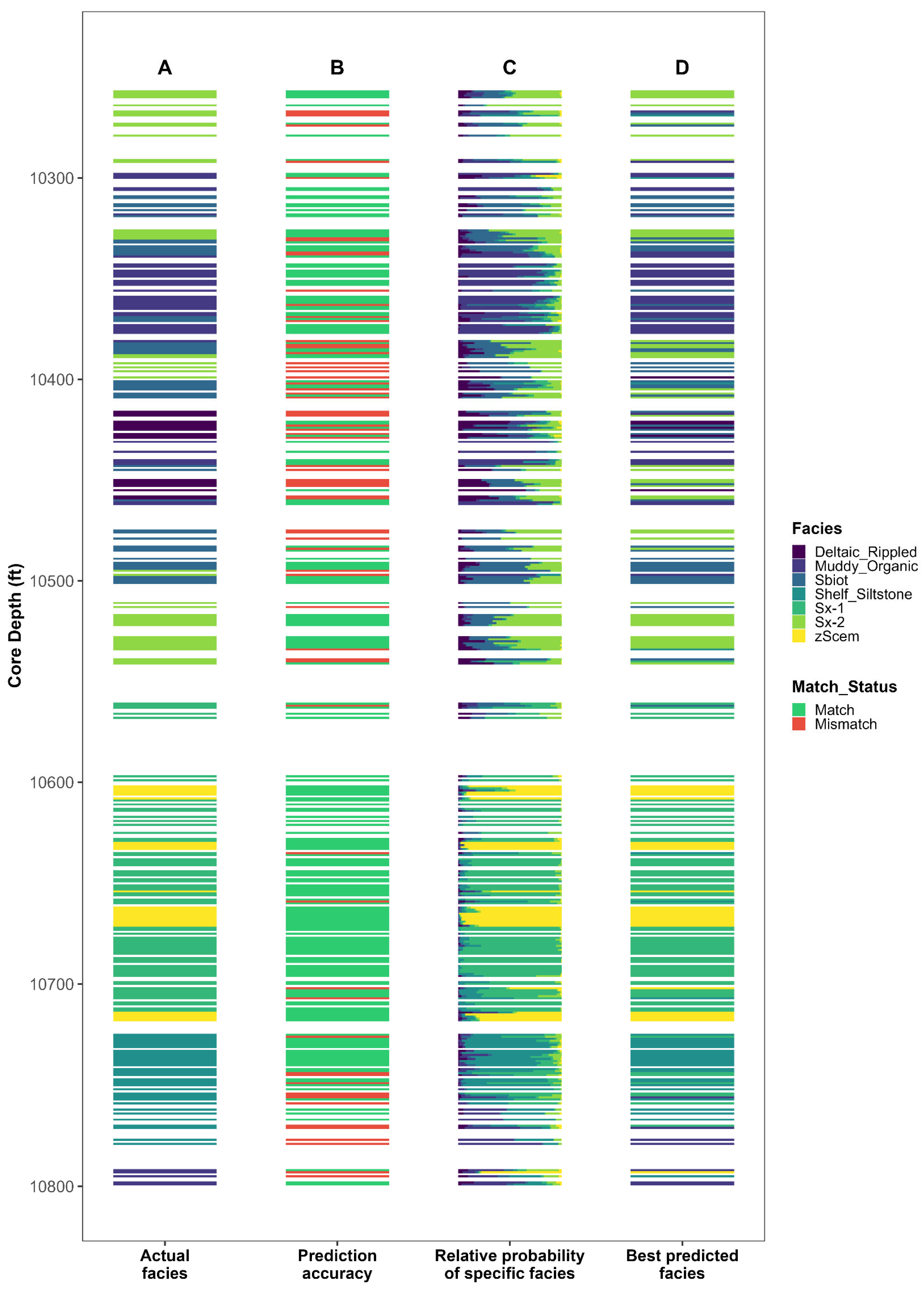
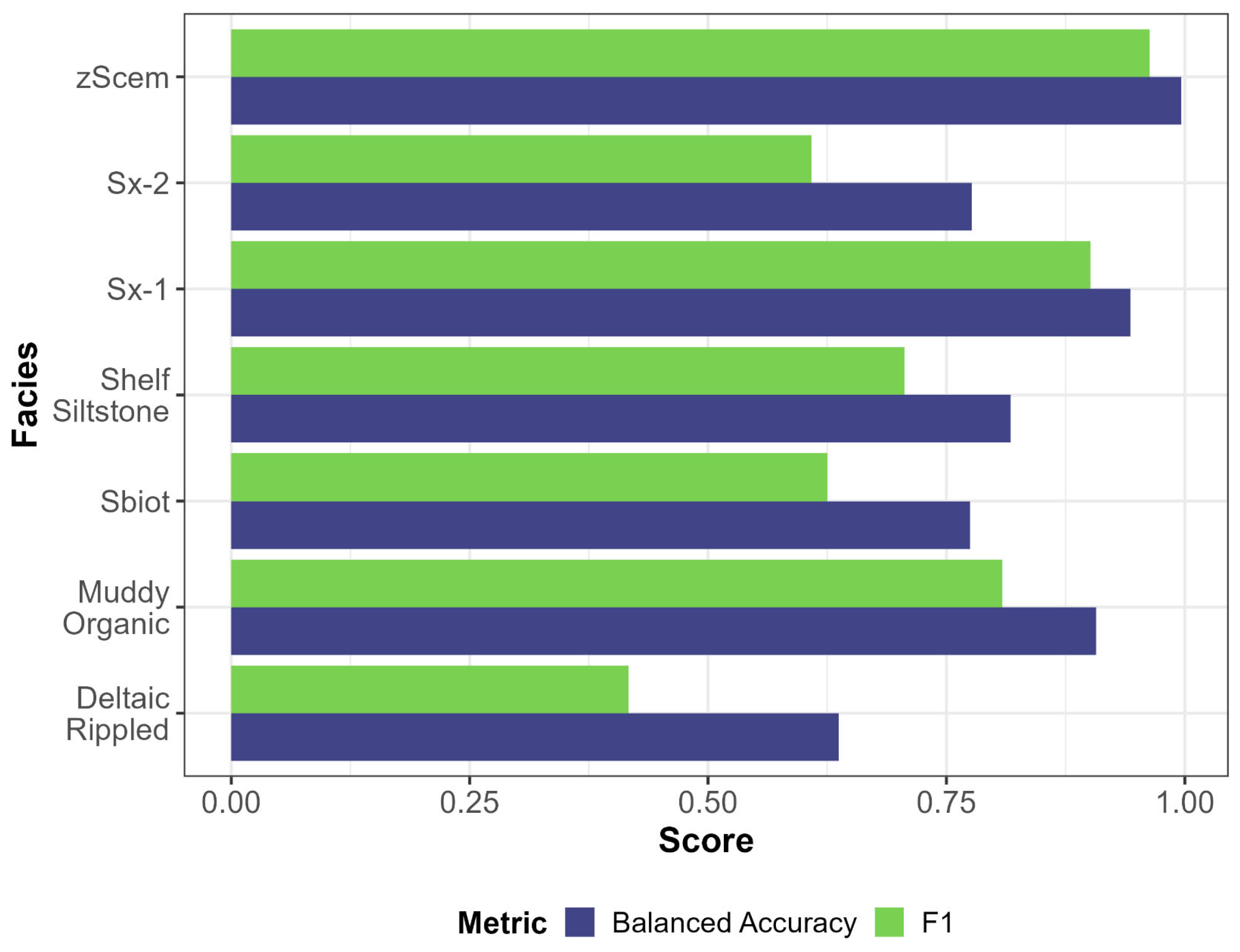
The validation log shows the core-described facies alongside the spatial distribution of correct and incorrect predictions and class probability profiles (Figure 21). Correct classifications are common throughout the Brent reservoir, with lower confidence and increased misclassification confined to specific stratigraphic levels where facies transitions are abrupt or the succession is strongly heterolithic. Class-specific balanced accuracy and F1 scores indicate that Sx-1 and Sx-2 sandstone facies achieve F1 scores of 0.95 and 0.85 respectively, whereas the deltaic rippled facies yield lower F1 values of around 0.55 (Figure 22).
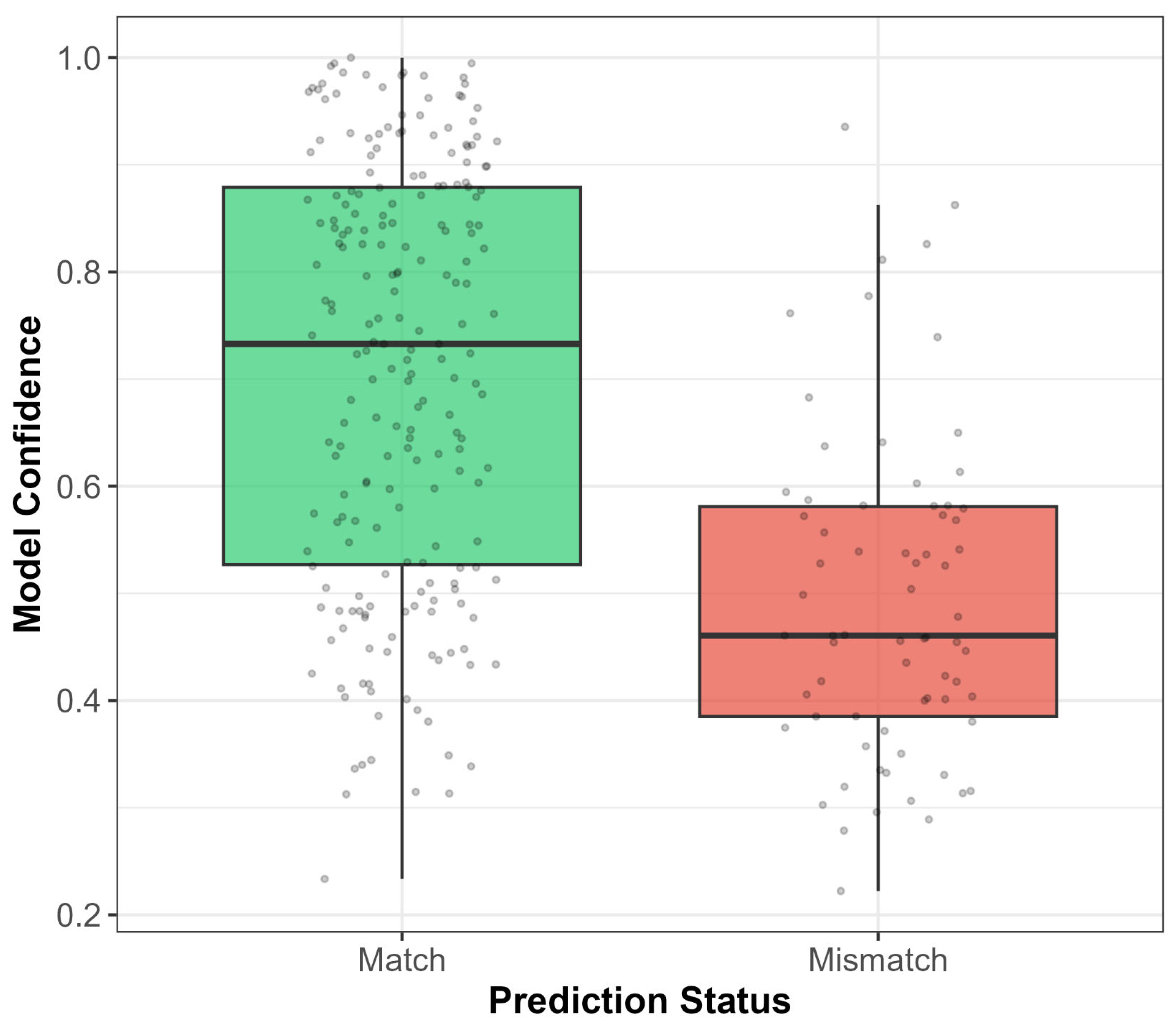
Model confidence scores are systematically higher for correctly classified samples than for incorrectly classified samples, and the calibration curve demonstrates that predicted probabilities are well calibrated, with mean observed accuracy tracking the 1:1 reference across most confidence bins (Figure 22 and Figure 23).
4. Discussion
The results show that bulk geochemical composition measured by HHXRF can recover petrophysical properties and facies architecture in the Brent Group with high fidelity. Random Forest models reproduce plug-scale porosity with high fidelity and directional permeability across several orders of magnitude (R2 > 0.95) and achieve substantial facies classification (κ ≈ 0.70), with best performance in clean sandstone facies. A consistent subset of elements (notably Ca, Ti, Si, V, Zn and Rb) dominates predictive skill across all targets, linking model behaviour to mineralogy, depositional texture and diagenesis rather than to purely statistical artefacts. Together, these findings indicate that rapid, low-cost HHXRF measurements, treated within a compositional data analysis and Random Forest framework, can provide a practical geochemical proxy for reservoir quality and facies organisation in quartz-rich siliciclastic reservoirs, particularly in settings where core is unavailable or sparse.
Figure 21.
Stratigraphic validation logs for the Random Forest facies classifier. (Panel A): baseline core-described facies. (Panel B): prediction accuracy (green = correct classification, red = misclassification). (Panel C): relative probability distribution across all seven facies classes at each depth interval, displayed as stacked bars. (Panel D): best-predicted facies class. The multi-track layout enables assessment of model performance in stratigraphic context and identification of depth intervals with elevated prediction uncertainty.
4.1. Predictive Value of HHXRF Compositional Data
The results show that HHXRF-derived major and trace element compositions can recover plug-scale porosity and permeability with high accuracy and can classify facies with substantial agreement, as evidenced by the tight clustering of measured versus predicted values in the porosity and permeability crossplots (Figure 6, Figure 10 and Figure 14) and the confusion matrix for facies classification (Figure 19). This extends earlier work that used geochemistry primarily for provenance, lithology and weathering reconstructions by demonstrating direct prediction of petrophysical and facies attributes from compositional data alone. Such applications build on the long tradition of using geochemical logs and core measurements to infer mineralogy and lithology [2,3,5,6,7], but move beyond qualitative interpretation to quantitative, plug-scale prediction supported by stratigraphic comparisons of measured and predicted properties (Figure 8, Figure 12 and Figure 16).
Figure 22.
Class-specific reliability metrics for the Random Forest facies classifier. Balanced accuracy and F1 scores are shown for each of the seven facies classes, derived from the out-of-bag confusion matrix. Balanced accuracy is the arithmetic mean of sensitivity and specificity; the F1 score is the harmonic mean of precision and recall. These metrics highlight which lithofacies are reliably predicted and which are systematically misclassified.
In the Brent Group specifically, numerous studies have characterised sedimentology, facies architecture and diagenesis using conventional core description, petrography and bulk geochemistry [9,12,13,15,16,17,19,20,22,23,60]. The present study complements this body of work by showing that a relatively small set of centred log-ratio (CLR)-transformed elements is sufficient to reconstruct both reservoir quality and facies classes at the plug positions, as shown by the variable importance profiles for porosity, permeability and facies (Figure 7, Figure 11, Figure 15 and Figure 20). In doing so, it points to workflows where continuous or high-density HHXRF scanning of core or cuttings can be exploited for rapid, quantitative subsurface characterisation, with stratigraphic logs of predictions and residuals providing a direct means to integrate geochemical ML outputs into established sedimentological frameworks.
4.2. Machine Learning in Geoscience and Comparison with Log-Based Prediction
Random Forest has become a standard tool for non-linear regression and classification in many disciplines because it handles complex predictor–response relationships, mixed predictor types and noisy data with minimal tuning [37,40,61]. In reservoir studies, a few machine-learning applications to date have focused on predicting permeability or facies from well logs and seismic attributes rather than from geochemistry, with recent work on chlorite-bearing sandstone reservoirs showing that supervised learning applied to wireline log suites can yield robust permeability and facies predictions at uncored depths [31].
The performance achieved here for porosity and permeability prediction from geochemical data is comparable to, and in some cases exceeds, that obtained from log-based models reported in the literature, with coefficients of determination of 0.95–0.96 and low RMSE values relative to the observed ranges (Figure 6, Figure 10 and Figure 14). This suggests that compositional data contain much of the information needed to reconstruct petrophysical properties, consistent with the strong mineralogical and diagenetic controls on reservoir quality in the Brent Group [9,19,22]. The dominance of a restricted element subset in the importance plots for both porosity and permeability (Figure 7, Figure 11 and Figure 15) reinforces this interpretation. The facies classification accuracy of approximately 75% and substantial Kappa values are consistent with other geoscientific Random Forest classification studies where classes overlap in attribute space and are defined on integrated sedimentological criteria [31,48,62], and the class-wise reliability metrics (Figure 22) confirm that facies-level prediction skill is comparable to log-based classifiers.
Figure 23.
Distribution of model confidence scores stratified by prediction outcome. Boxplots overlaid with jittered individual data points (i.e., small circles) show confidence score distributions for correctly classified samples (green, matches) and misclassified samples (red, mismatches). Higher confidence scores for correct predictions and lower scores for incorrect predictions indicate good model calibration. The small degree of overlap between distributions reflects the degree to which confidence scores can discriminate between reliable and unreliable predictions.
4.3. Compositional Data Treatment and Model Interpretability
A key methodological aspect of this work is the explicit treatment of elemental concentrations as compositional data, using CLR transformation to remove the closure constraint and permit valid multivariate analysis in Euclidean space [32,33,34,36,63]. Compositional approaches have been widely advocated in environmental and sedimentary geochemistry because they avoid spurious correlations induced by the constant-sum constraint and allow interpretation in terms of relative element enrichments [1,4,7]. The strong performance of the RF models here suggests that the CLR-transformed predictors provide an appropriate representation of geochemical variability for data-driven reservoir characterisation.
Variable importance analyses consistently highlight Ca, Ti and Si as the most influential predictors across porosity, permeability and facies models, with Zn, V, K, S, Sr and Rb also making substantial contributions (Figure 7, Figure 11, Figure 15 and Figure 20). While RF importance measures must be interpreted cautiously due to potential biases, particularly when predictors are correlated [44,45], the use of permutation-based percentage increase in mean squared error (%IncMSE) together with significance testing via rfPermute provides a more robust ranking than impurity measures alone [41], and the consistency of dominant elements across the three models further supports their geological relevance. The surrogate decision tree aids interpretability by revealing approximate compositional thresholds associated with specific facies and reservoir quality regimes (Figure 18), providing a bridge between the ensemble and more traditional rule-based geological reasoning. This complements the confusion matrix, stratigraphic validation log and confidence-calibration plots as a suite of diagnostic tools (Figure 19, Figure 20, Figure 21, Figure 22 and Figure 23).
4.4. Geological Controls on Model Performance
The element suite identified as most important is consistent with current understanding of Brent Group mineralogy and diagenesis. Ca likely reflects variations in carbonate cementation, which are known to exert a major control on porosity and permeability in the Brent Group, especially the Rannoch Formation [20,21,23], and this inference is supported by the association between Ca-rich intervals and reduced porosity and permeability in the stratigraphic prediction panels (Figure 9 and Figure 13). Ti and by association high-field-strength elements often track heavy-mineral and clay-rich components and thus capture facies-dependent variations in detrital input and diagenetic alteration [7,24,64]. Si serves as a proxy for detrital quartz content and quartz cementation, both of which strongly influence mechanical compaction and pore structures [9,19,22], consistent with the high importance of Si across all four RF models (Figure 7, Figure 11, Figure 15 and Figure 20).
The facies-stratified residuals for both porosity and permeability models indicate that prediction errors are not uniformly distributed across facies, with high-quality sandstone facies (e.g., Sx-1, Sx-2 and Sbiot) tending to show tighter residual distributions and higher F1 scores, while heterolithic or mud-rich facies (Shelf-Siltstone, Muddy-Organic, Deltaic-Rippled) display broader residual ranges and lower classification performance (Figure 9, Figure 13, Figure 17 and Figure 22). This pattern likely reflects greater internal heterogeneity in grain size, sorting and cementation within the latter facies, which may not be fully captured by a single point measurement of HHXRF on the core surface, and is mirrored in the stratigraphic validation log where misclassifications and low-confidence predictions cluster around heterolithic intervals and facies transitions (Figure 21). This pattern also emphasises the importance of integrating sedimentological context, including facies architecture and stacking patterns, with geochemical and machine-learning outputs [9,12,13,17]. Depth-aligned plots of predictions, residuals and facies (Figure 8, Figure 12, Figure 16 and Figure 21) provide that integrative framework.
4.5. Methodological Limitations and Sources of Uncertainty
Despite the strong crossplots and favourable performance metrics, several limitations must be acknowledged. First, the training and validation dataset come from a single, well-characterised Brent Group succession in one field, so model extrapolation to other fields, basins or lithostratigraphic intervals requires caution and additional calibration [15,18,30], ideally through application of the trained workflow to further wells and comparison of prediction performance on independent crossplots and stratigraphic logs analogous to those presented here. Sediment provenance, burial history, diagenetic pathways and operational factors such as core handling can all alter the relationship between composition and petrophysical properties [9,22,23,24]; the main conclusions are currently confined to quartz-rich, moderately buried, marginal marine siliciclastics with similar diagenetic histories.
Second, HHXRF analysis introduces several sources of uncertainty. The instrument cannot quantify elements lighter than Mg and has relatively high detection limits for some light elements [6,7,8,65], so the models necessarily ignore components such as clay-bound water and organic matter that may influence pore structure. Core-surface measurements also sample a small, potentially heterogeneous area adjacent to each plug and may be affected by roughness, saw-marks or minor contamination, so they are only an approximation to true plug-volume composition. These factors likely contribute to the facies-dependent residual patterns we observe, with larger errors in heterolithic and carbonate-cemented intervals (e.g., Figure 8, Figure 9, Figure 12 and Figure 13). However, the overall predictive performance and the consistent importance of a restricted suite of elements (Figure 7, Figure 11 and Figure 15) suggest that these measurement uncertainties do not obscure the primary compositional controls on porosity, permeability and facies in this dataset. Partial remedies are available: for example integrating HHXRF with a small number of complementary measurements, loss-on-ignition or carbonate content by acid digestion for the organic and carbonate fractions, and total clay by XRD at selected intervals, would allow the most influential unquantified components to be incorporated as additional predictors, and would provide a direct test of whether their inclusion reduces the facies-dependent residual patterns observed here.
Third, the use of out-of-bag validation provides an efficient and largely unbiased error estimate [42,43,66], but independent blind validation on separate wells or cuttings datasets, with crossplots, confusion matrices and calibration curves (e.g., Figure 6, Figure 10, Figure 14 and Figure 19), would provide a stronger test of model generalisation. We therefore regard the OOB metrics as internally robust but still preliminary, pending blind application to independent wells/cuttings.
Fourth, the Random Forest models treat each sample as independent and do not explicitly encode stratigraphic ordering, spatial correlation or measurement uncertainty. As a result, they cannot capture hierarchical structure such as bed-scale trends, stacking patterns or depth-dependent diagenetic overprints that might systematically modify the relationship between composition, porosity and permeability. The largely structureless residuals with depth for porosity and horizontal permeability (Figure 8 and Figure 12) and the facies-segregated residual distributions (Figure 9 and Figure 13) suggest that this omission does not strongly bias the present results, but it may limit the ability to extrapolate predictions into intervals with markedly different facies stacking or burial histories. A practical first step would be to incorporate stratigraphic position, formation membership or normalised depth within a sequence stratigraphic framework, as an additional predictor, which would allow the RF models to account for systematic depth-dependent diagenetic trends without requiring a fundamentally different modelling architecture. Longer-term, embedding the compositional predictors within spatially explicit models such as Gaussian process regression or geostatistical co-simulation frameworks would allow prediction uncertainty to be propagated directly into geocellular models, providing spatially coherent estimates of porosity and permeability with quantified confidence intervals rather than the sample-wise OOB metrics reported here.
Taken together, these limitations constrain the scope of our inferences but do not alter the central conclusion that HHXRF-derived composition encodes the dominant controls on reservoir quality and facies architecture in this Brent Group example.
4.6. Comparison with Previous Studies
Studies that have explicitly combined compositional data analysis with machine learning for subsurface applications remain relatively rare, but a few recent contributions have been instructive. Meloni et al. [67] integrated compositional data analysis (CoDA) with Random Forest to define lithology-specific geochemical baselines in heterogeneous volcanic–sedimentary terrains, using CLR/ILR-transformed soil geochemistry to achieve robust lithological classification and outlier-resistant baselines. Their approach is conceptually similar to the present facies classification in that both rely on tree-based ensembles trained on transformed geochemical compositions, but Meloni et al. did not attempt to predict porosity or permeability, nor did they apply the integrated stratigraphic validation employed here (Figure 8, Figure 12, Figure 16 and Figure 21).
More directly relevant to reservoir characterisation, Nourani et al. [68] used handheld XRF elemental data and a suite of machine-learning models, including Random Forest, to predict porosity in chalk samples, and showed that XRF-based models could match or exceed more traditional multivariate approaches for porosity prediction. Their predictors were elemental compositions, but the data were not treated as compositional; nor did they include facies classification, variable importance analysis across multiple targets, or surrogate-tree-based interpretability. Al-Khudafi et al. [69] applied multiple tree-based classifiers, including Random Forest and decision trees, to wireline log data for facies determination in the Gamal/Camal oilfields and found that Random Forest systematically outperformed alternative tree algorithms for lithology identification, but their inputs were conventional logs rather than geochemical compositions, and they did not address porosity or permeability prediction or integrate predictions into stratigraphic panels.
In contrast, the present study applied CLR transformation to HHXRF-derived elemental compositions prior to modelling, respecting the compositional nature of the predictors, and used Random Forest to predict porosity, permeability in log-space and seven facies classes from the same compositional feature set. By integrating compositional data analysis with Random Forest in a reservoir-quality context, and combining petrophysical regression, facies classification, permutation-based variable importance and surrogate trees within a single workflow (Figure 6, Figure 7, Figure 8, Figure 9, Figure 10, Figure 11, Figure 12, Figure 13, Figure 14, Figure 15, Figure 16, Figure 17, Figure 18, Figure 19, Figure 20, Figure 21, Figure 22 and Figure 23), we have, for the first time, extended earlier geochemical-baseline and XRF-porosity studies into a unified compositional framework for quantitative prediction of both reservoir properties and facies architecture in siliciclastic sandstones.
4.7. Implications for Energy-Transition Subsurface Characterisation
From an applied perspective, the ability to derive porosity, directional permeability and facies from rapid, low-cost HHXRF measurements has clear implications for subsurface characterisation in support of carbon capture and storage (CCS), underground hydrogen storage and geothermal projects. Wireline logs can also be used to derive porosity but (1) the XRF approach yields comparable results without requiring log acquisition and (2) an important outcome of this approach is that directional permeability can be predicted from XRF analyses of cuttings samples in uncored well intervals or in nearby uncored wells penetrating the same stratigraphic interval. Note that wireline logs cannot be used to derive permeability directly, making this XRF approach a valuable source of petrophysical data where core is unavailable.
For CCS, improved quantification of reservoir quality and facies architecture in both saline aquifers and depleted hydrocarbon fields is central to storage capacity estimates, injectivity predictions and long-term containment assessments [25]. The depth-aligned predictions and residuals presented here (Figure 8, Figure 9, Figure 12, Figure 13, Figure 16 and Figure 17) show how XRF-driven machine-learning outputs can be embedded directly into the stratigraphic and facies frameworks used for such assessments. Similarly, for underground hydrogen storage, accurate mapping of permeability structure and sealing facies is critical to ensure deliverability and minimise leakage risk [26], and the class-wise performance metrics for sealing versus high-permeability facies (Figure 21 and Figure 22) demonstrate that compositional data can support such discrimination.
The workflows demonstrated here suggest that where core is available, XRF-based models could be trained and then deployed on cuttings or additional cores to populate geocellular models in uncored intervals, potentially in combination with wireline log-based machine-learning predictions [30,31]. The facies confidence and calibration information (Figure 19, Figure 20, Figure 21 and Figure 22) can additionally be used to weight or filter predictions when propagating them into static and dynamic reservoir models. This integrated approach, combining compositional geochemistry with machine learning, aligns with broader moves towards unified digital subsurface frameworks for energy-transition projects, in which geological, petrophysical and geochemical datasets are combined to reduce uncertainty [27,29]. The present results provide a worked example of how HHXRF-ML outputs can be visualised and interrogated in stratigraphic context (Figure 5, Figure 8, Figure 12, Figure 16 and Figure 21). Future work should extend the present models to multi-well datasets, explore transfer learning between fields, and evaluate how prediction uncertainty, as quantified by residual distributions and confidence scores, propagates into dynamic flow simulations and risk assessments for CCS, hydrogen storage and geothermal developments.
5. Conclusions
- XRF-derived compositional data can accurately predict plug-scale porosity and permeability using Random Forest models with high accuracy (R2 > 0.95, low RMSE), showing that bulk composition captures the dominant controls on reservoir quality in this Brent Group succession.
- The same compositional data support robust classification into seven facies classes, with substantial agreement with core-described facies (κ = 0.705) and reliable recovery of the main sandstone and heterolithic associations.
- A small subset of elements, notably Ca, Ti and Si with contributions from several trace elements, dominates predictive capability for both petrophysical properties and facies, linking model behaviour to mineralogy, depositional texture and diagenetic modification.
- Prediction performance is facies dependent: clean, well-sorted sandstone facies are reproduced more reliably than heterolithic or mud-rich facies, and residual patterns in these latter facies reflect more complex, small-scale compositional and textural heterogeneity.
- Stratigraphic plots show that the models capture key vertical trends in reservoir quality while highlighting intervals where composition–property relationships are more complex, providing a geochemically constrained view of facies architecture and reservoir quality variations through the Brent succession.
- Out-of-bag validation and confidence calibration indicate that prediction uncertainties are well-behaved, enabling the use of model confidence to screen low-reliability classifications and focus interpretation on the most robust predictions.
- The workflow demonstrates that rapid, relatively low-cost XRF measurements can be integrated into digital reservoir characterisation, providing high-resolution inputs for populating geocellular models in CCS, hydrogen storage and geothermal projects, as well as in conventional oil and gas reservoirs, particularly in uncored or data-sparse intervals.
Author Contributions
Conceptualisation, R.H.W. and A.Y.L.; Methodology, R.H.W. and A.Y.L.; Software, R.H.W. and A.Y.L.; Validation, R.H.W. and A.Y.L.; Formal analysis, R.H.W. and A.Y.L.; Investigation, R.H.W. and A.Y.L.; Resources, R.H.W. and A.Y.L.; Data curation, R.H.W. and A.Y.L.; Writing—original draft, R.H.W. and A.Y.L.; Writing—review and editing, R.H.W. and A.Y.L.; Visualisation, R.H.W. and A.Y.L.; Supervision, R.H.W.; Project administration, R.H.W.; Funding acquisition, R.H.W. and A.Y.L. All authors have read and agreed to the published version of the manuscript.
Funding
We would like to thank the Nigerian government’s Petroleum Technology Development Fund for providing funding for the sedimentary logging and XRF analysis parts of this research project.
Data Availability Statement
The original contributions presented in this study are included in the article. The four sets of R codes to model and predict facies, porosity, horizontal permeability and vertical permeability plus the original XRF and related data are available at https://zenodo.org/records/20204927 (accessed on 15 May 2026). Further inquiries can be directed to the corresponding author.
Acknowledgments
The authors have reviewed and edited the output and take full responsibility for the content of this publication. We thank the journal reviewers for their supportive comments. We would like to express appreciation to the University of Liverpool’s Emma Michie for her useful suggestions about subtle changes in expression.
Conflicts of Interest
The authors declare no conflicts of interest. The funders had no role in the design of the study; in the collection, analyses, or interpretation of data; in the writing of the manuscript; or in the decision to publish the results.
References
- Andersson, P.O.D.; Worden, R.H. Mudstones of the Tanqua Basin, South Africa: An analysis of lateral and stratigraphic variations within mudstones, and a comparison of mudstones within and between turbidite fans. Sedimentology 2004, 51, 479–502. [Google Scholar] [CrossRef] [Scilit]
- Herron, M.M. Geochemical classification of terrigenous sands and shales from core or log data. J. Sediment. Petrol. 1988, 58, 820–829. [Google Scholar]
- Herron, M.M. Mineralogy from geochemical well logging. Clays Clay Miner. 1986, 34, 204–213. [Google Scholar] [CrossRef] [Scilit]
- Nesbitt, H.W.; Young, G. Early Proterozoic climates and plate motions inferred from major element chemistry of lutites. Nature 1982, 299, 715. [Google Scholar] [CrossRef] [Scilit]
- Rothwell, R.G. Micro-XRF studies of sediment cores: A perspective on capability and application in the environmental sciences. In Micro-XRF Studies of Sediment Cores; Croudace, I.W., Rothwell, R.G., Eds.; Springer: Berlin, Germany, 2015; pp. 1–21. [Google Scholar]
- Turner, J.N.; Jones, A.F.; Brewer, P.A.; Macklin, M.G.; Rassner, S.M. Micro-XRF applications in fluvial sedimentary environments of Britain and Ireland: Progress and prospects. In Micro-XRF Studies of Sediment Cores; Croudace, I.W., Rothwell, R.G., Eds.; Springer: Berlin, Germany, 2015; pp. 227–265. [Google Scholar]
- Rollinson, H.R. Using Geochemical Data: Evaluation, Presentation, Interpretation; Routledge: Abingdon, UK, 2014. [Google Scholar]
- Schillereff, D.N.; Chiverrell, R.C.; Croudace, I.W.; Boyle, J.F. An inter-comparison of µXRF scanning analytical methods for lake sediments. In Micro-XRF Studies of Sediment Cores; Croudace, I.W., Rothwell, R.G., Eds.; Springer: Berlin, Germany, 2015; pp. 583–600. [Google Scholar]
- Lawan, A.Y.; Worden, R.H.; Utley, J.E.P.; Crowley, S.F. Sedimentological and diagenetic controls on the reservoir quality of marginal marine sandstones buried to moderate depths and temperatures: Brent Province, UK North Sea. Mar. Pet. Geol. 2021, 128, 104993. [Google Scholar] [CrossRef] [Scilit]
- Williams, R.R.; Milne, A.D. The Thistle Field, Blocks 211/18a and 211/19, UK North Sea. In United Kingdom Oil and Gas Fields 25 Years Commemorative Volume; Abbotts, I.L., Ed.; The Geological Society Memoirs; The Geological Society: London, UK, 1991; Volume 14, pp. 199–207. [Google Scholar]
- Bayat, M.G.; Tehrani, D.H. The Thistle Field―Analysis of Its Past Performance and Optimisation of Its Future Development. In Proceedings of the Offshore Europe, Aberdeen, UK, 10 September 1985. [Google Scholar]
- Morris, J.; Hampson, G.J.; Maxwell, G. Controls on facies architecture in the Brent Group, Strathspey Field, UK North Sea: Implications for reservoir characterization. Pet. Geosci. 2003, 9, 209–220. [Google Scholar] [CrossRef] [Scilit]
- Brown, S.; Richards, P.C.; Thomson, A.R. Patterns in the deposition of the Brent Group (Middle Jurassic) UK North Sea. In Petroleum Geology of North West Europe; Brooks, J., Glennie, K.W., Eds.; The Geological Society of London: London, UK, 1987; pp. 899–913. [Google Scholar]
- Livera, S.E. Facies associations and sand-body geometries in the Ness Formation of the Brent Group, Brent Field. In Deltas: Sites and Traps for Fossil Fuels; Whateley, M.K.G., Pickering, K.T., Eds.; Geological Society Special Publications; The Geological Society: London, UK, 1989; Volume 41. [Google Scholar]
- Reynolds, A.D. Sedimentology and sequence stratigraphy of the Thistle Field, Northern North Sea. In Norwegian Petroleum Society Special Publications; Steel, R.J., Felt, V.L., Johannessen, E.P., Mathieu, C., Eds.; Elsevier: Amsterdam, The Netherlands, 1995; Volume 5, pp. 257–271. [Google Scholar]
- Cannon, S.J.C.; Giles, M.R.; Whitaker, M.F.; Please, P.M.; Martin, S.V. A regional assessment of the Brent Group, UK sector, North Sea. In Geology of the Brent Group. Special Publication; Morton, A.C., Haszeldine, R.S., Giles, M.R., Brown, S., Eds.; Geological Society Special Publications; The Geological Society: London, UK, 1992; Volume 61, pp. 81–107. [Google Scholar]
- Mitchener, B.C.; Lawrence, D.A.; Partington, M.A.; Bowman, M.B.J.; Gluyas, J. Brent Group: Sequence stratigraphy and regional implications. In Geology of the Brent Group. Special Publication; Morton, A.C., Haszeldine, R.S., Giles, M.R., Brown, S., Eds.; Geological Society Special Publications; The Geological Society: London, UK, 1992; Volume 61, pp. 45–80. [Google Scholar]
- Richards, P.C. An introduction to the Brent Group: A literature review. In Geology of the Brent Group. Special Publication; Morton, A.C., Haszeldine, R.S., Giles, M.R., Brown, S., Eds.; Geological Society Special Publications; The Geological Society: London, UK, 1992; Volume 61, pp. 15–26. [Google Scholar]
- Nedkvitne, T.; Bjørlykke, K. Secondary porosity in the Brent Group (Middle Jurassic), Huldra Field, North Sea: Implication for predicting lateral continuity of sandstones? J. Sediment. Petrol. 1992, 62, 23–34. [Google Scholar]
- Prosser, D.J.; Daws, J.A.; Fallick, A.E.; Williams, B.P.J. Geochemistry and diagenesis of stratabound calcite cement layers within the Rannoch Formation of the Brent Group, Murchison Field, North Viking Graben (Northern North Sea). Sediment. Geol. 1993, 87, 139–164. [Google Scholar] [CrossRef] [Scilit]
- Ashcroft, W.A.; Ridgway, M.S. Early discordant diagenesis in the Brent Group, Murchison Field, UK North Sea, detected in high values of seismic-derived acoustic impedance. Pet. Geosci. 1996, 2, 75–81. [Google Scholar] [CrossRef] [Scilit]
- Bjørlykke, K.; Nedkvitne, T.; Ramm, M.; Saigal, G. Diagenetic processes in the Brent Group (Middle Jurassic) reservoirs of the North Sea: An overview. In Geology of the Brent Group. Special Publication; Morton, A.C., Haszeldine, R.S., Giles, M.R., Brown, S., Eds.; Geological Society Special Publications; The Geological Society: London, UK, 1992; Volume 61, pp. 263–287. [Google Scholar]
- Harris, N.B. Burial diagenesis of Brent sandstones: A study of Statfjord, Hutton and Lyell fields. In Geology of the Brent Group. Special Publication; Morton, A.C., Haszeldine, R.S., Giles, M.R., Brown, S., Eds.; The Geological Society: London, UK, 1992; Volume 61, pp. 351–375. [Google Scholar]
- Morton, A.C. Provenance of Brent Group sandstones: Heavy mineral constraints. In Geology of the Brent Group. Special Publication; Morton, A.C., Haszeldine, R.S., Giles, M.R., Brown, S., Eds.; Geological Society Special Publications; The Geological Society: London, UK, 1992; Volume 61, pp. 227–244. [Google Scholar]
- Worden, R.H. Carbon dioxide capture and storage (CCS) in saline aquifers versus depleted gas fields. Geosciences 2024, 14, 146. [Google Scholar] [CrossRef] [Scilit]
- Miocic, J.; Heinemann, N.; Edlmann, K.; Scafidi, J.; Molaei, F.; Alcaldi, J. Underground hydrogen storage: A review. In Enabling Secure Subsurface Storage in Future Energy Systems, Special Publication; Miocic, J., Heinemann, N., Edlmann, K., Alcalde, J., Schultz, R., Eds.; The Geological Society: London, UK, 2023; Volume 528, pp. 73–86. [Google Scholar]
- Storey, B.M.; Worden, R.H.; McNamara, D.D.; Wheeler, J.; Parker, J.; Kristen, A. Reactivation of Abandoned Oilfields for Cleaner Energy Generation: Three-Dimensional Modelling of Reservoir Heterogeneity and Geometry. Processes 2024, 12, 2883. [Google Scholar] [CrossRef] [Scilit]
- Storey, B.M.; Worden, R.H.; McNamara, D.D. The Geoscience of In-Situ Combustion and High-Pressure Air Injection. Geosciences 2022, 12, 340. [Google Scholar] [CrossRef] [Scilit]
- Turner, J.P.; Berry, T.W.; Bowman, M.J.; Chapman, N.A. The role of the geosphere in deep nuclear waste disposal―England and Wales perspective. Earth Sci. Rev. 2023, 242, 104445. [Google Scholar] [CrossRef] [Scilit]
- Cannon, S. Petrophysics―A Practical Guide; Wiley: Chichester, UK, 2016. [Google Scholar]
- Nichols, T.E.; Worden, R.H.; Houghton, J.E.; Griffiths, J.; Brostrom, C.; Martinius, A.W. Machine Learning for Reservoir Quality Prediction in Chlorite-Bearing Sandstone Reservoirs. Geosciences 2025, 15, 325. [Google Scholar] [CrossRef] [Scilit]
- Aitchison, J. The Statistical Analysis of Compositional Data; Chapman and Hall: London, UK, 1986. [Google Scholar]
- Aitchison, J.; Greenacre, M. Biplots of compositional data. J. R. Stat. Soc. Ser. C Appl. Stat. 2002, 51, 375–392. [Google Scholar] [CrossRef] [Scilit]
- Pawlowsky-Glahn, V.; Egozcue, J.J. Compositional data and their analysis: An introduction. In Compositional Data Analysis in the Geosciences: From Theory to Practice; Buccianti, A., Mateu-Figueras, G., Pawlowsky-Glahn, V., Eds.; Special Publications; The Geological Society: London, UK, 2006; Volume 264, pp. 1–10. [Google Scholar]
- Martín-Fernández, J.A.; Barceló-Vidal, C.; Pawlowsky-Glahn, V. Dealing with zeros and missing values in compositional data sets using nonparametric imputation. Math. Geol. 2003, 35, 253–278. [Google Scholar] [CrossRef] [Scilit]
- Pawlowsky-Glahn, V.; Egozcue, J.J.; Tolosana-Delgado, R. Modeling and Analysis of Compositional Data; John Wiley & Sons: Chichester, UK, 2015. [Google Scholar]
- Breiman, L. Random forests. Mach. Learn. 2001, 45, 5–32. [Google Scholar] [CrossRef] [Scilit]
- Efron, B. Bootstrap methods: Another look at the jackknife. Ann. Stat. 1979, 7, 1–26. [Google Scholar] [CrossRef] [Scilit]
- Jensen, J.L.; Hinkley, D.V.; Lake, L.W. A statistical study of reservoir permeability: Distributions, correlations, and averages. SPE Reserv. Eval. Eng. 2000, 3, 461–468. [Google Scholar] [CrossRef] [Scilit]
- Liaw, A.; Wiener, M. Classification and regression by random forest. R News 2002, 2, 18–22. [Google Scholar]
- Archer, E. rfPermute: Estimate Permutation p-Values for Random Forest Importance Metrics. R package version 2.5.2. Available online: https://CRAN.R-project.org/package=rfPermute (accessed on 15 April 2026).
- Bylander, T. Estimating generalization error on two-class datasets using out-of-bag estimates. Mach. Learn. 2002, 48, 287–297. [Google Scholar] [CrossRef] [Scilit]
- Janitza, S.; Hornung, R. On the overestimation of random forest’s out-of-bag error. PLoS ONE 2018, 13, e0201904. [Google Scholar] [CrossRef] [Scilit]
- Strobl, C.; Boulesteix, A.-L.; Zeileis, A.; Hothorn, T. Bias in random forest variable importance measures: Illustrations, sources and a solution. BMC Bioinform. 2007, 8, 25. [Google Scholar] [CrossRef] [Scilit]
- Altmann, A.; Toloşi, L.; Sander, O.; Lengauer, T. Permutation importance: A corrected feature importance measure. Bioinformatics 2010, 26, 1340–1347. [Google Scholar] [CrossRef] [Scilit]
- Cohen, J. A coefficient of agreement for nominal scales. Educ. Psychol. Meas. 1960, 20, 37–46. [Google Scholar] [CrossRef] [Scilit]
- Landis, J.R.; Koch, G.G. The measurement of observer agreement for categorical data. Biometrics 1977, 33, 159–174. [Google Scholar] [CrossRef] [Scilit]
- Powers, D.M.W. Evaluation: From precision, recall and F-measure to ROC, informedness, markedness and correlation. J. Mach. Learn. Technol. 2011, 2, 37–63. [Google Scholar]
- Niculescu-Mizil, A.; Caruana, R. Predicting good probabilities with supervised learning. In Proceedings of the 22nd International Conference on Machine Learning (ICML); Association for Computing Machinery: Bonn, Germany, 2005; pp. 625–632. [Google Scholar]
- Therneau, T.; Atkinson, B. rpart: Recursive Partitioning and Regression Trees. R Package Version 4.1.19. Available online: https://CRAN.R-project.org/package=rpart (accessed on 13 March 2026).
- Molnar, C. Interpretable Machine Learning: A Guide for Making Black Box Models Explainable, 3rd ed.; Leanpub: Victoria, BC, Canada, 2025. [Google Scholar]
- R Core Team. R: A Language and Environment for Statistical Computing. Available online: https://www.R-project.org/ (accessed on 13 January 2026).
- Kuhn, M. Building predictive models in R using the caret package. J. Stat. Softw. 2008, 28, 1–26. [Google Scholar] [CrossRef] [Scilit]
- Wickham, H.; François, R.; Henry, L.; Müller, K.; Vaughan, D. dplyr: A Grammar of Data Manipulation. R Package Version 1.1.2. Available online: https://CRAN.R-project.org/package=dplyr (accessed on 15 April 2026).
- Wickham, H. ggplot2: Elegant Graphics for Data Analysis; Springer: Cham, Switzerland, 2016; p. 226. [Google Scholar]
- Milborrow, S. rpart.plot: Plot ‘rpart’ Models: An Enhanced Version of ‘plot.rpart’. R Package Version 3.1.1. Available online: https://CRAN.R-project.org/package=rpart.plot (accessed on 5 February 2026).
- Garnier, S.; Ross, N.; Rudis, R.; Camargo, A.P.; Sciaini, M.; Scherer, C. viridis: Colorblind-Friendly Color Maps for R. R Package Version 0.6.3. Available online: https://CRAN.R-project.org/package=viridis (accessed on 15 December 2025).
- Pedersen, T.L. Patchwork: The Composer of Plots. R Package Version 1.1.2. Available online: https://CRAN.R-project.org/package=patchwork (accessed on 1 March 2026).
- Godefroy, S.; Korb, J.P.; Fleury, M.; Bryant, R.G. Surface nuclear magnetic relaxation and dynamics of water and oil in porous media. Phys. Rev. E 2001, 64, 021605. [Google Scholar] [CrossRef] [Scilit]
- Richards, P.C.; Brown, S. The Nature of the Brent Delta, North Sea: A Core Workshop; Open File Report; British Geological Survey: London, UK, 1987. [Google Scholar]
- Hastie, T.; Tibshirani, R.; Friedman, J. The Elements of Statistical Learning: Data Mining, Inference, and Prediction, 2nd ed.; Springer: New York, NY, USA, 2009. [Google Scholar]
- Brodersen, K.H.; Ong, C.S.; Stephan, K.E.; Buhmann, J.M. The balanced accuracy and its posterior distribution. In Proceedings of the 2010 20th International Conference on Pattern Recognition; IEEE: New York, NY, USA, 2010; pp. 3121–3124. [Google Scholar]
- Filzmoser, P.; Hron, K.; Reimann, C. Univariate statistical analysis of environmental (compositional) data: Problems and possibilities. Sci. Total Environ. 2009, 407, 6100–6108. [Google Scholar] [CrossRef] [Scilit]
- Andersson, P.O.D.; Worden, R.H.; Hodgson, D.M.; Flint, S. Provenance evolution and chemostratigraphy of a Palaeozoic submarine fan-complex: Tanqua Karoo Basin, South Africa. Mar. Pet. Geol. 2004, 21, 555–577. [Google Scholar] [CrossRef] [Scilit]
- Rothwell, R.G.; Croudace, I.W. Twenty years of XRF core scanning marine sediments: What do geochemical proxies tell us? In Micro-XRF Studies of Sediment Cores: Applications of a Non-Destructive Tool For the Environmental Sciences; Developments in Paleoenvironmental Research; Croudace, I.W., Rothwell, R.G., Eds.; Springer: Dordrecht, The Netherlands, 2015; Volume 17, pp. 25–102. [Google Scholar]
- Breiman, L. Bagging predictors. Mach. Learn. 1996, 24, 123–140. [Google Scholar] [CrossRef] [Scilit]
- Meloni, F.; Gozzi, C.; Cabassi, J.; Nisi, B.; Rappuoli, D.; Vaselli, O. Integrating Compositional Data Analysis (CoDA) and Random Forest for lithology-specific geochemical baseline determination. Sci. Total Environ. 2026, 1011, 181169. [Google Scholar] [CrossRef] [Scilit]
- Nourani, M.; Alali, N.; Samadianfard, S.; Band, S.S.; Chou, K.-W.; Shu, C.-M. Comparison of machine learning techniques for predicting porosity of chalk. J. Pet. Sci. Eng. 2022, 209, 109853. [Google Scholar] [CrossRef] [Scilit]
- Al-Khudafi, A.M.; Hamada, G.M.; Al-gathe, A.; Farea, I.A.; Baarimah, S.O. Tree-based machine learning can determine lithofacies properties of reservoir rocks―Camal oil field, Yemen. Egypt. J. Pet. 2024, 33, 450–460. [Google Scholar] [CrossRef] [Scilit]
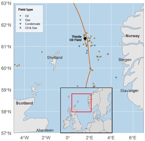
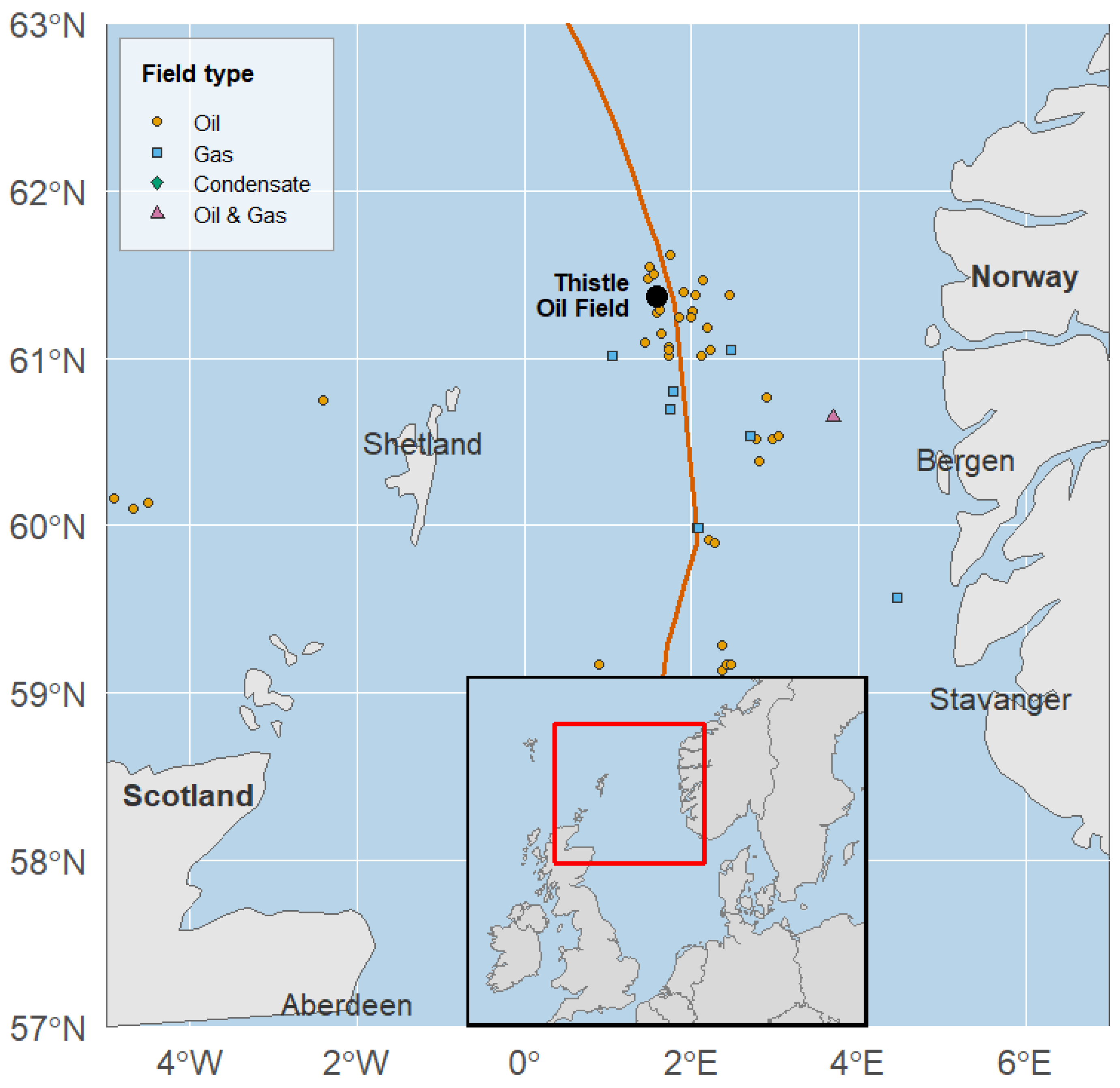
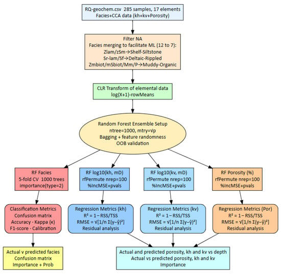
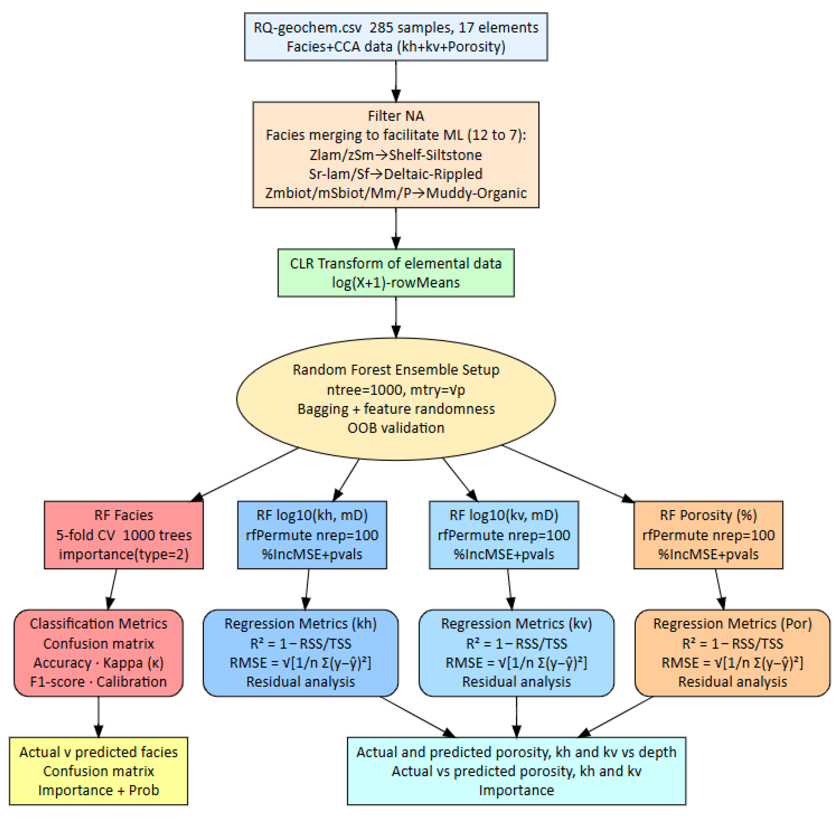
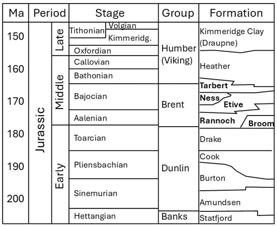
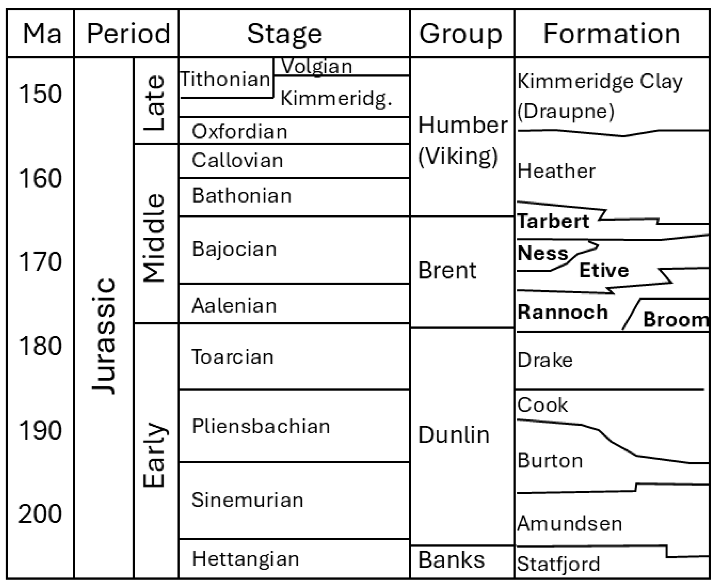
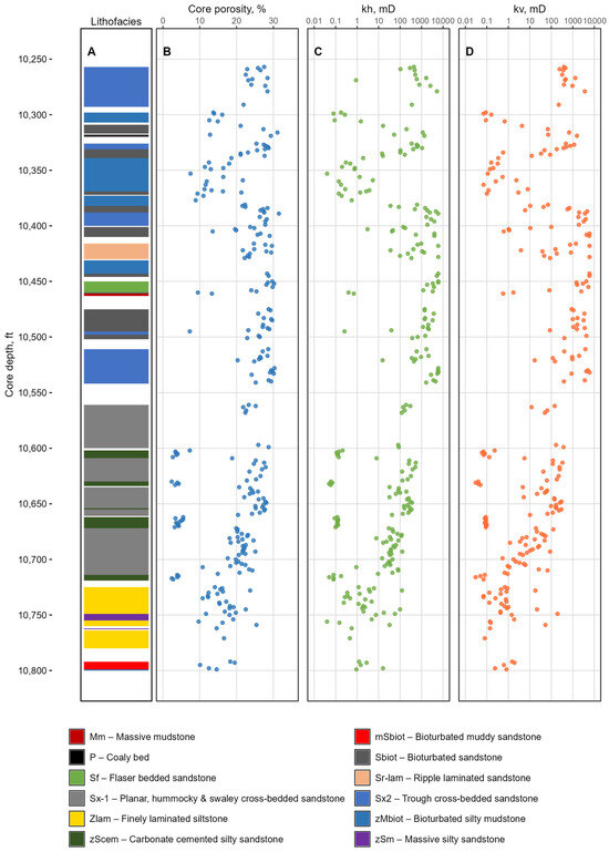
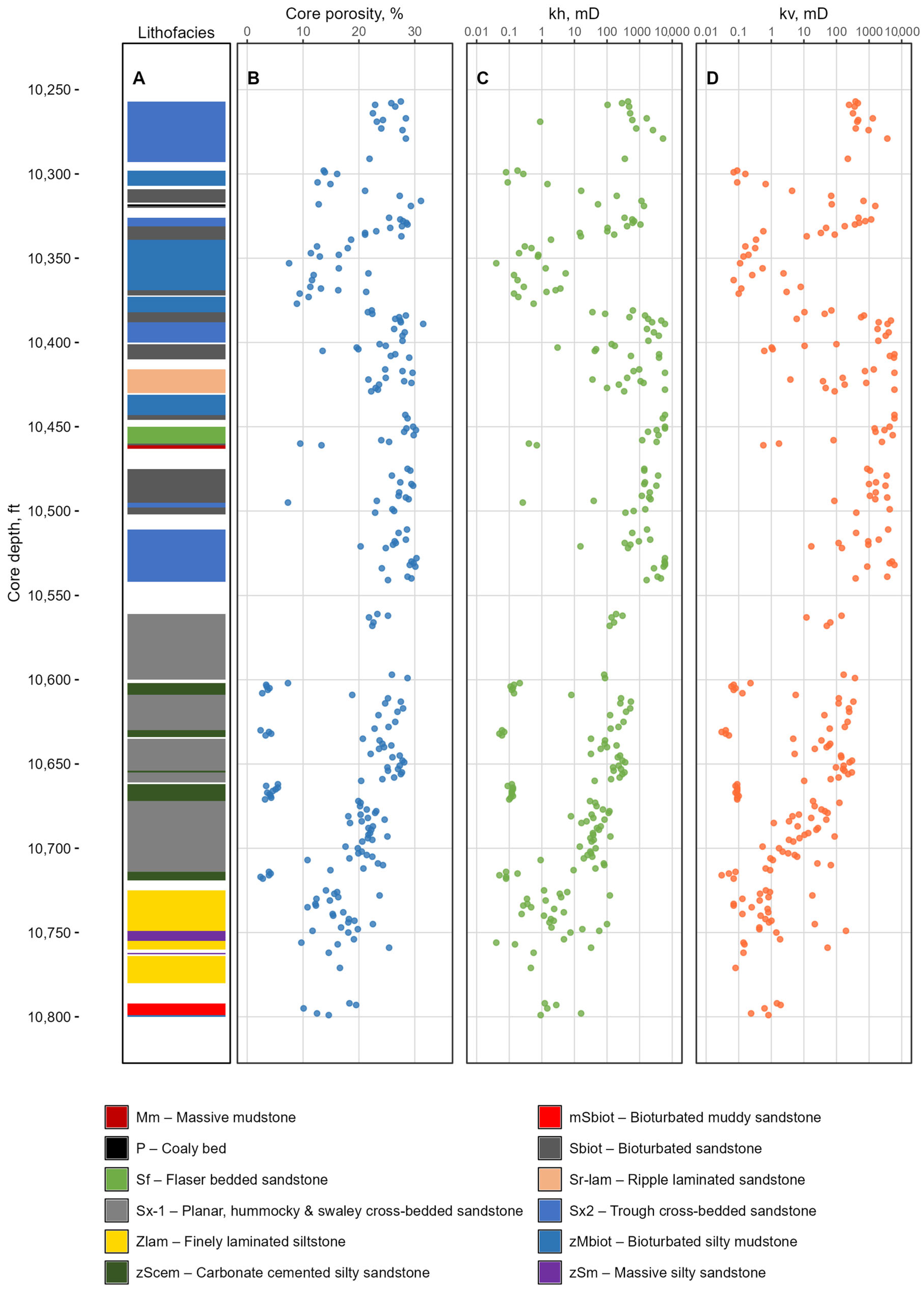
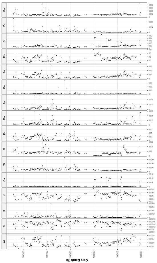
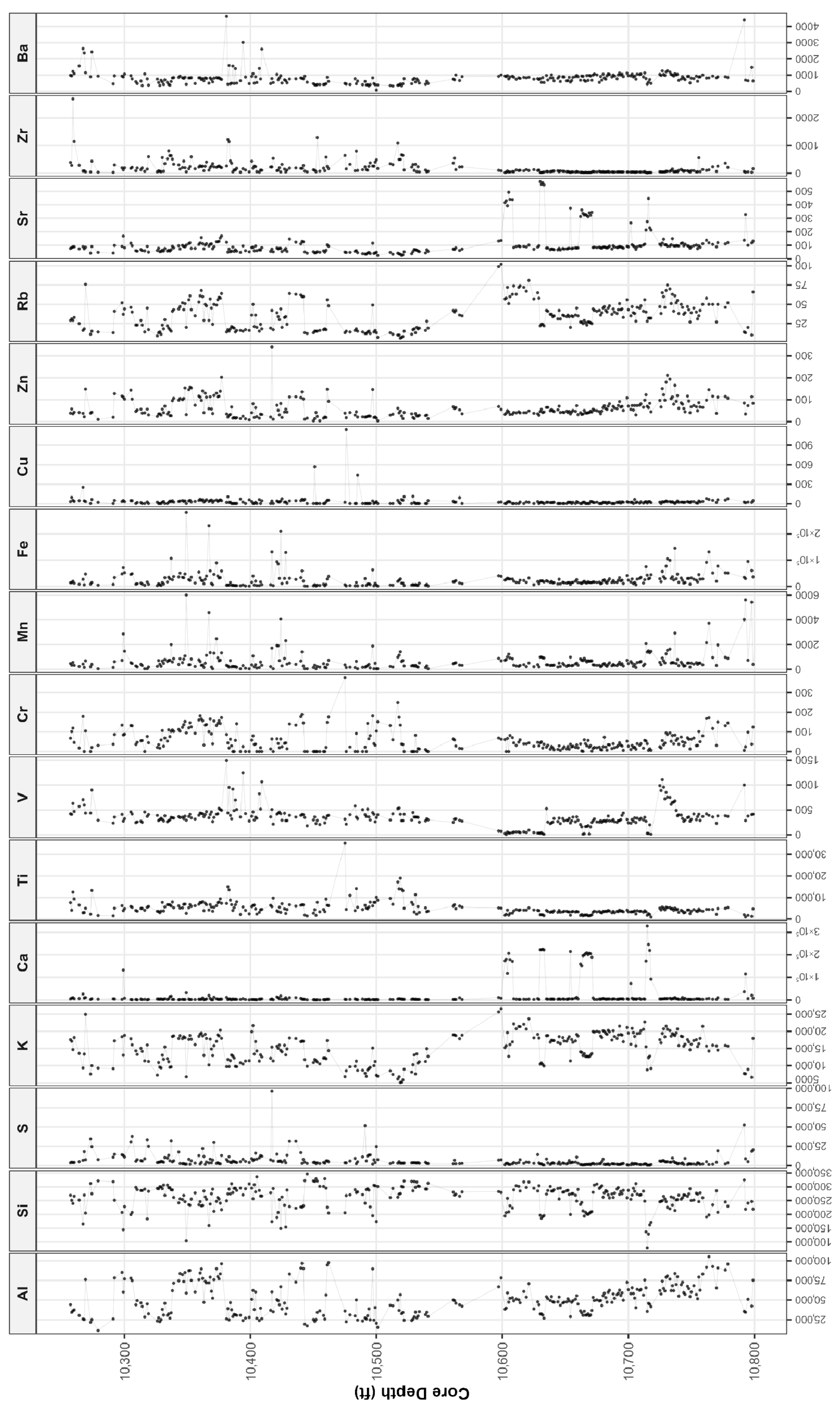
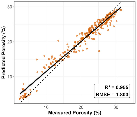
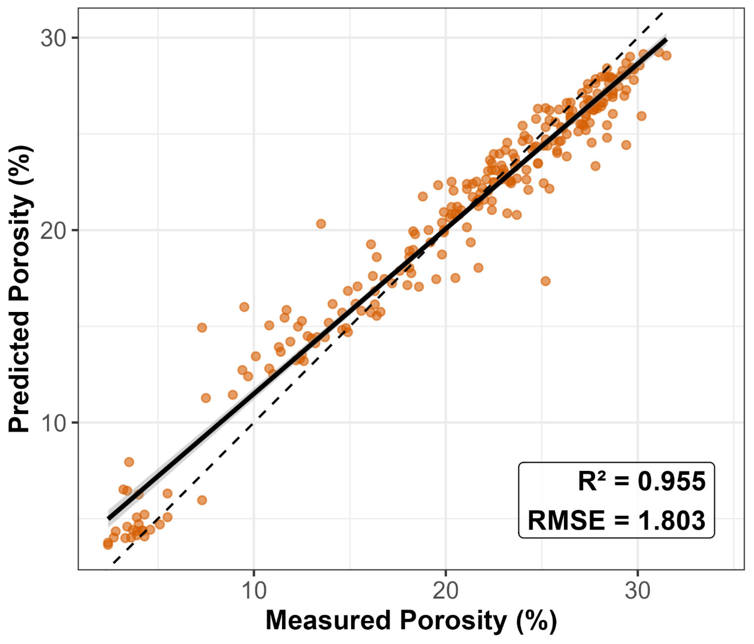
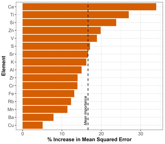
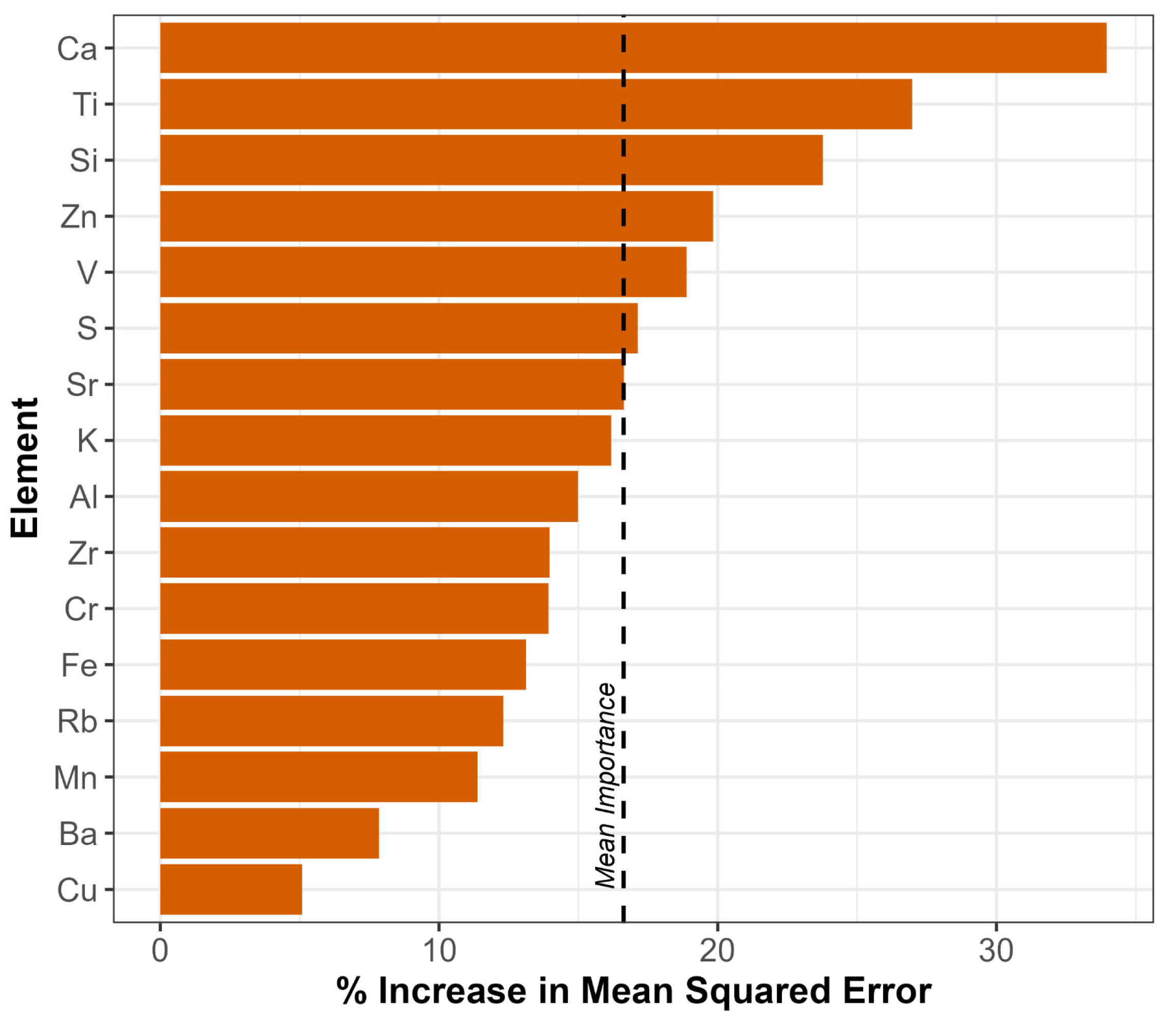
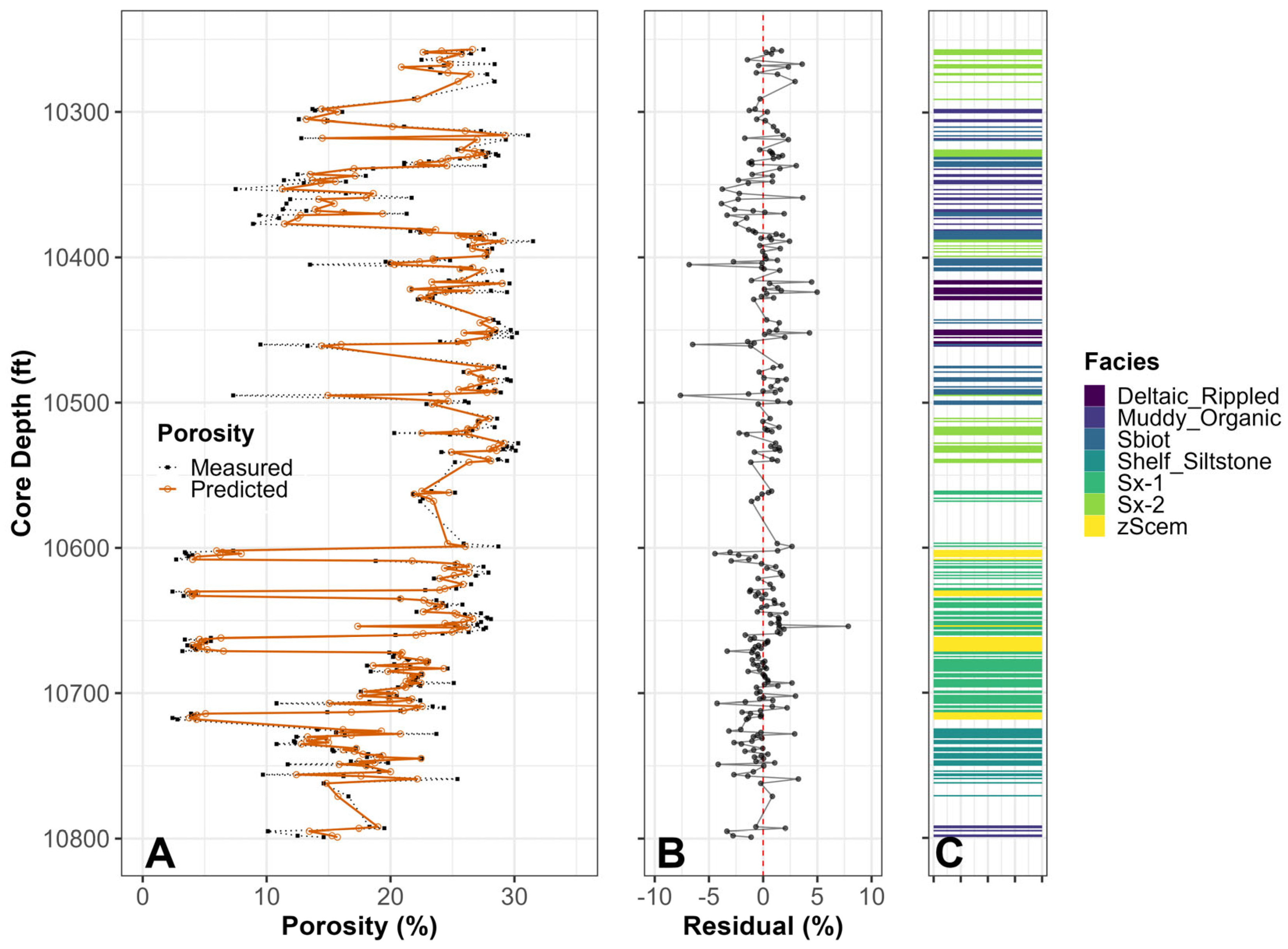
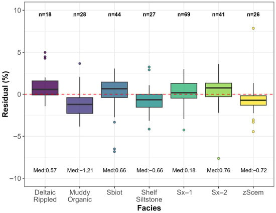
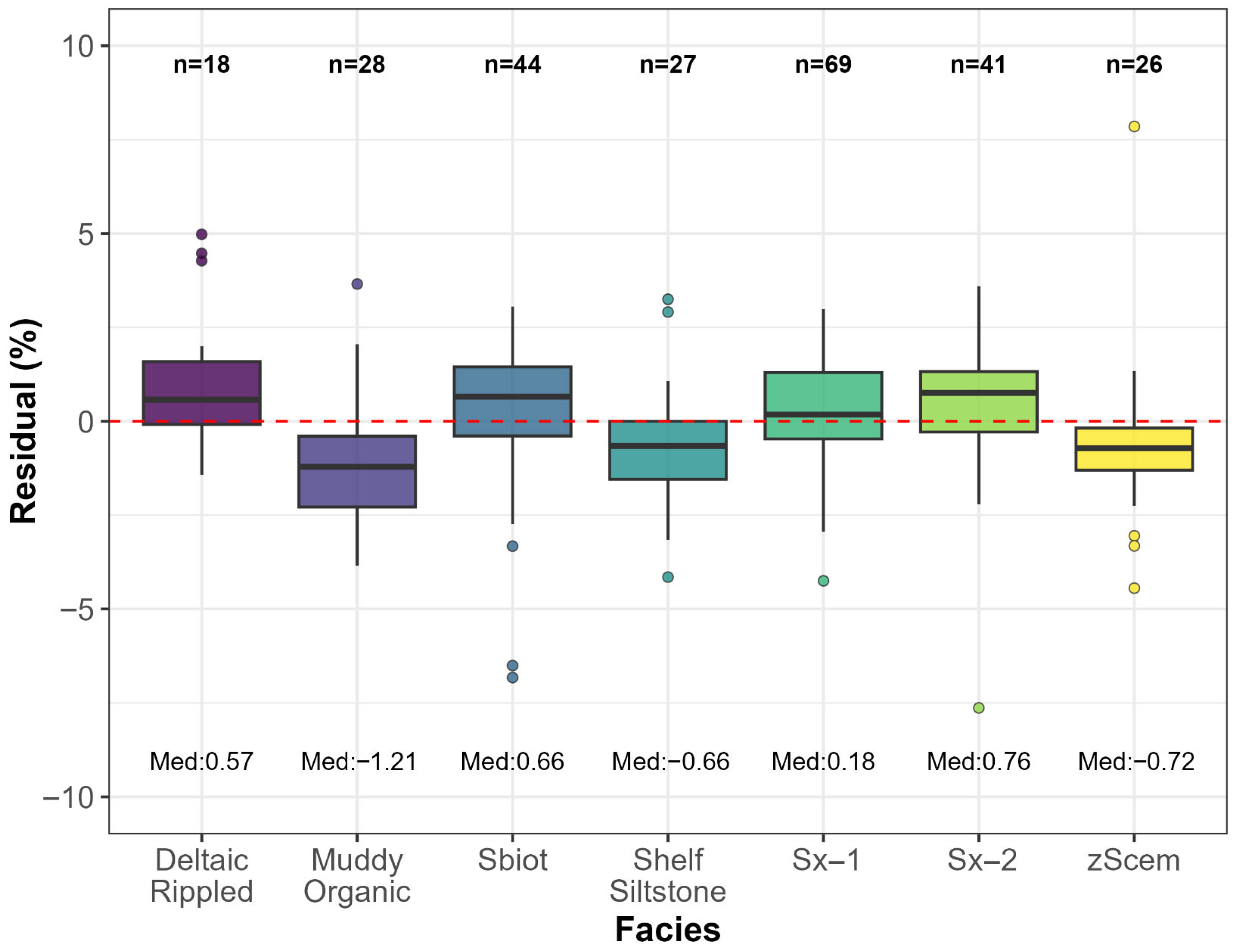
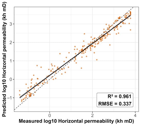
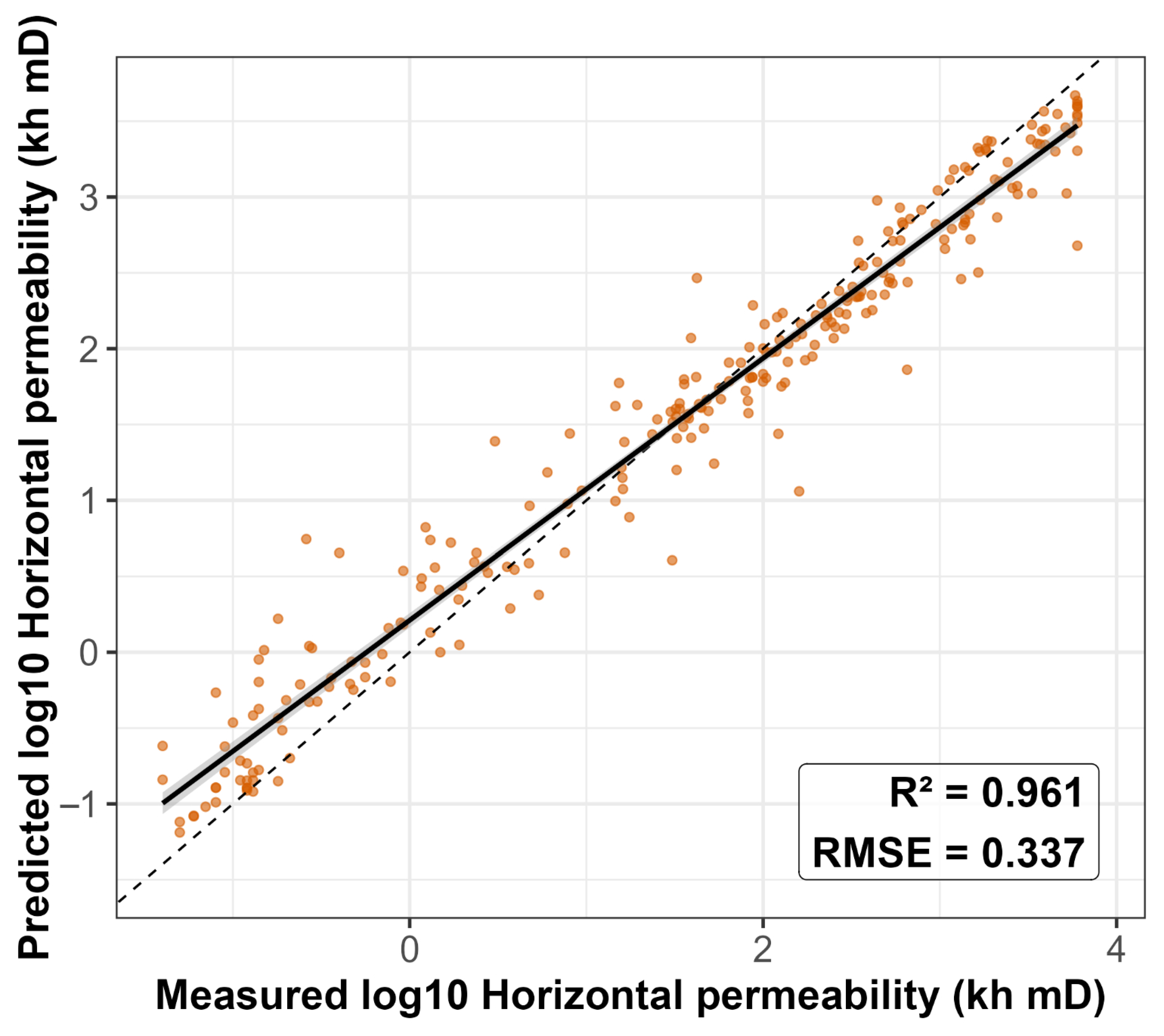
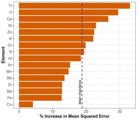
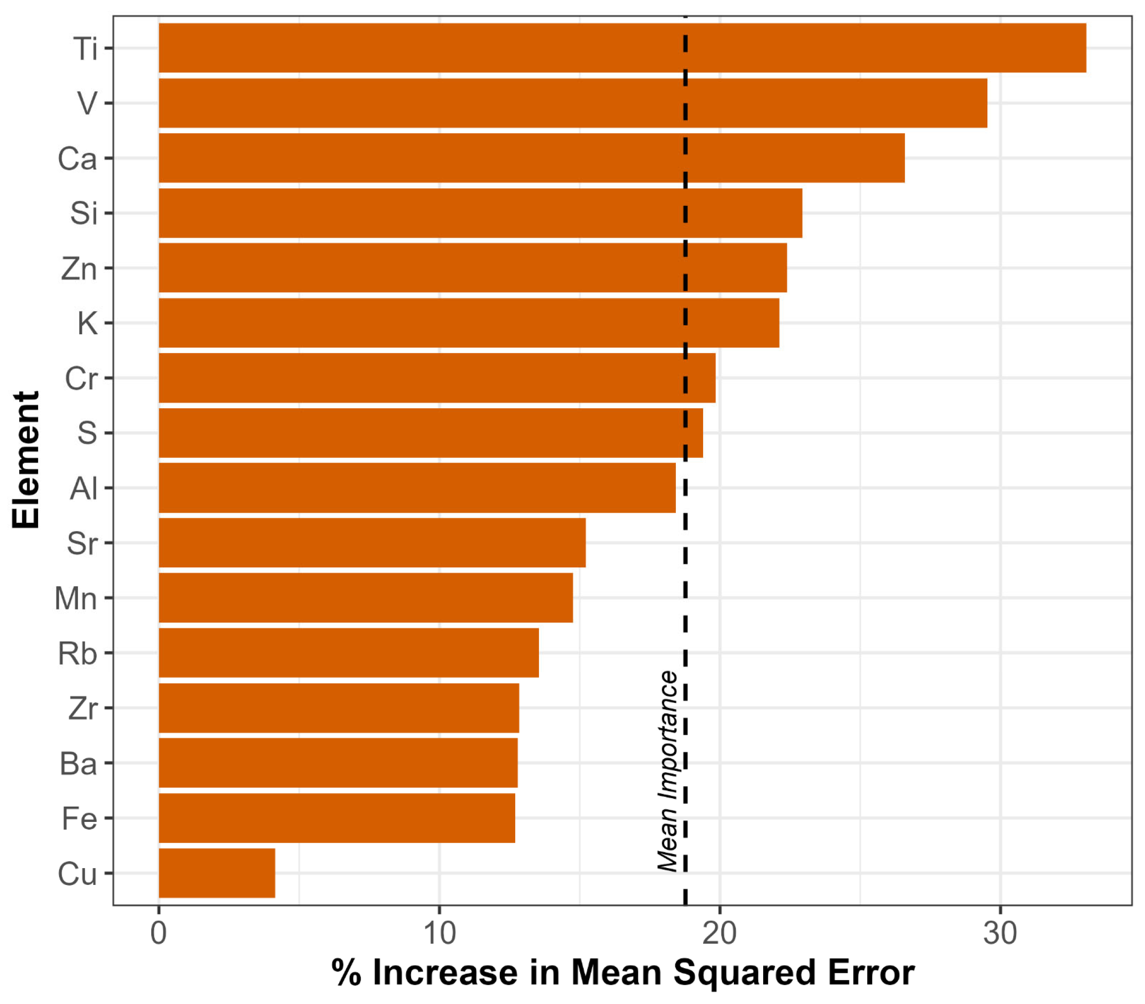
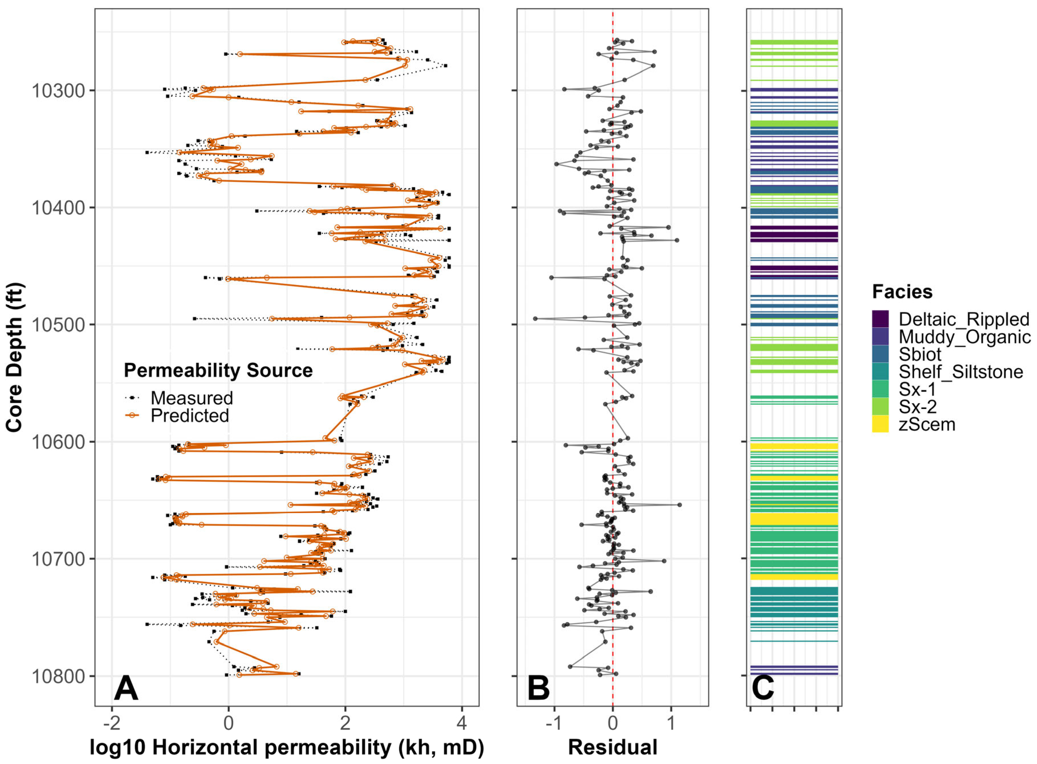
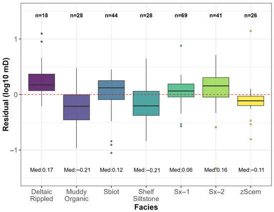
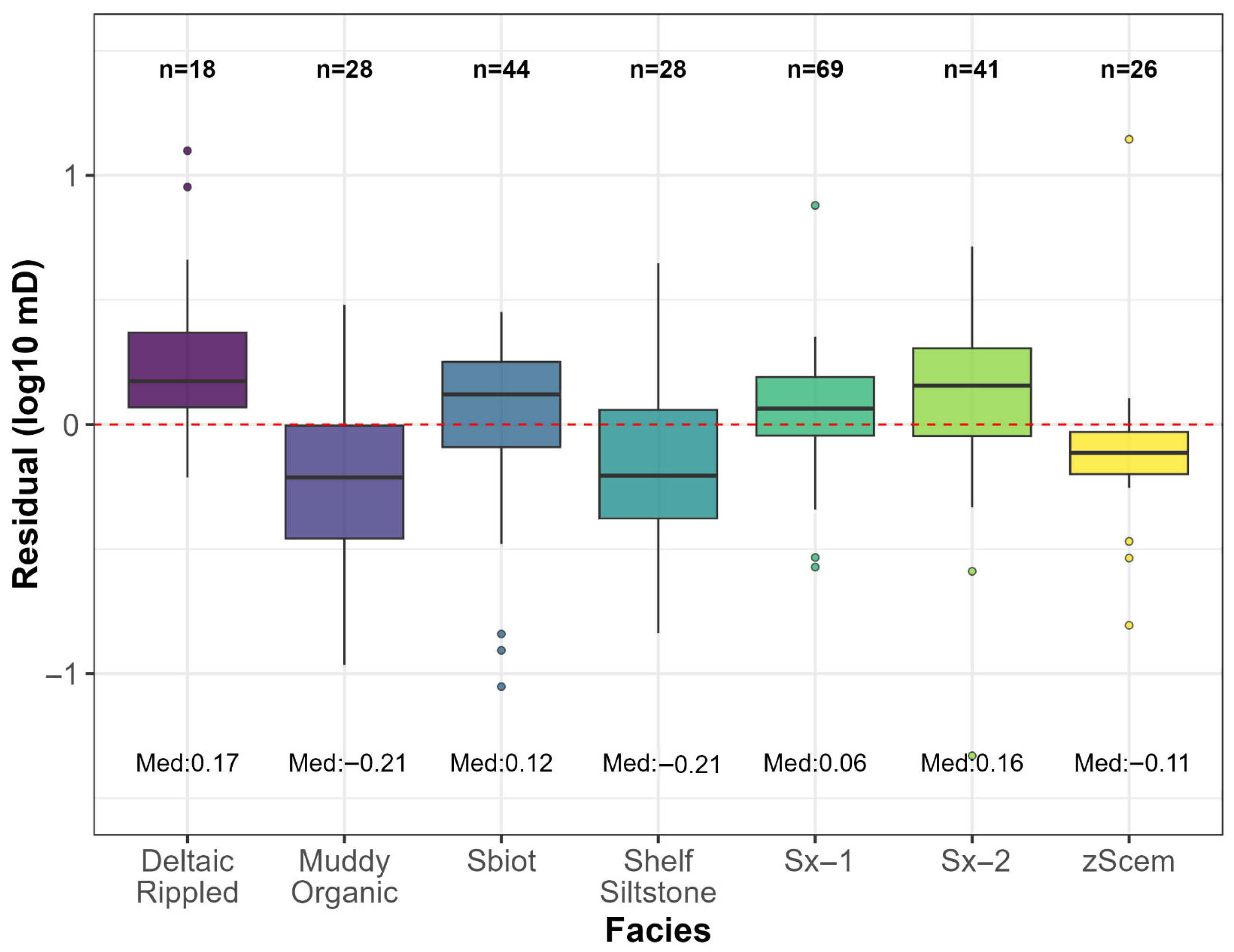
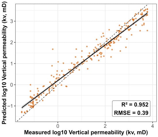
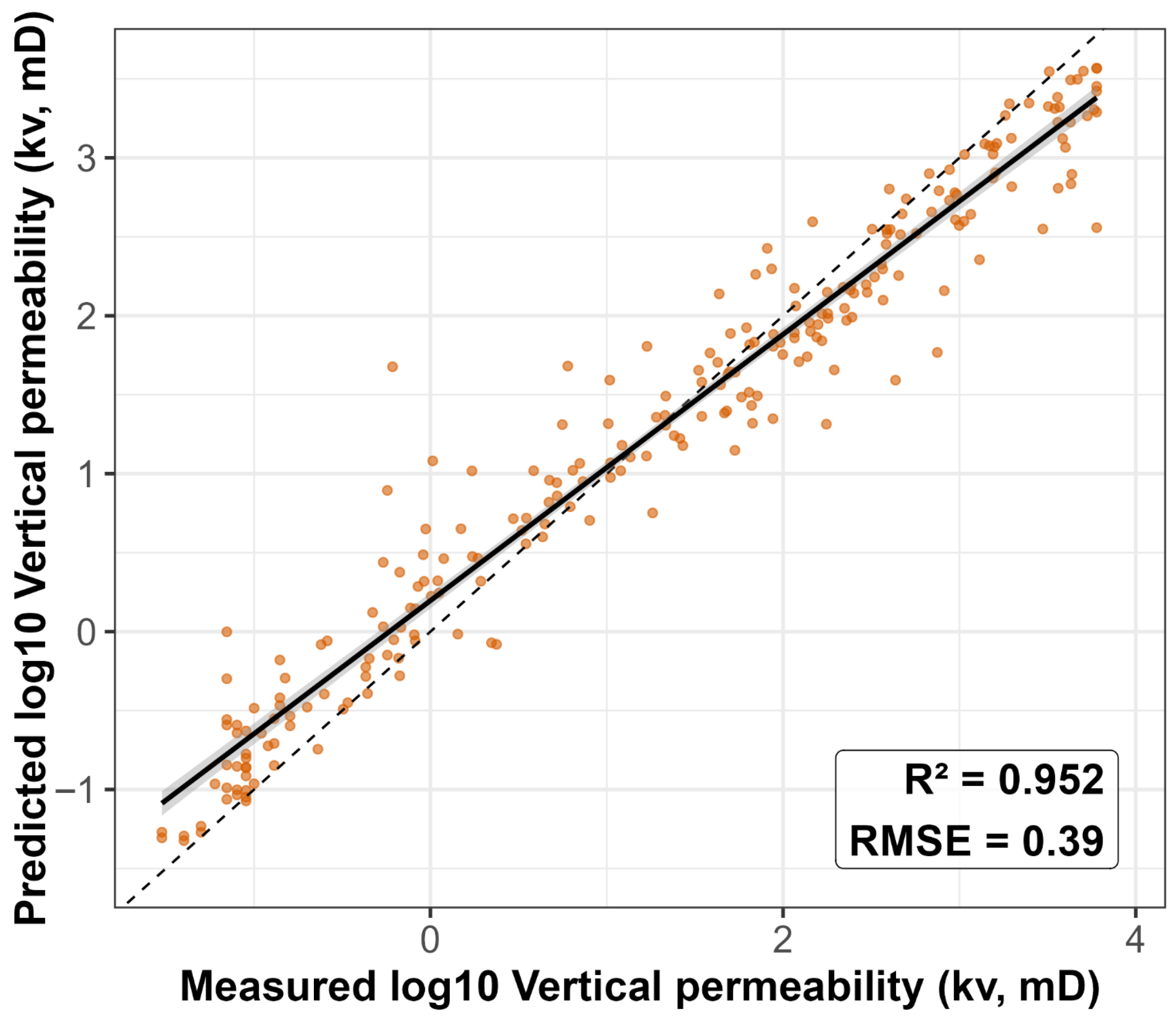
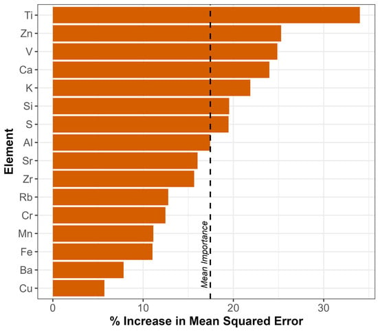
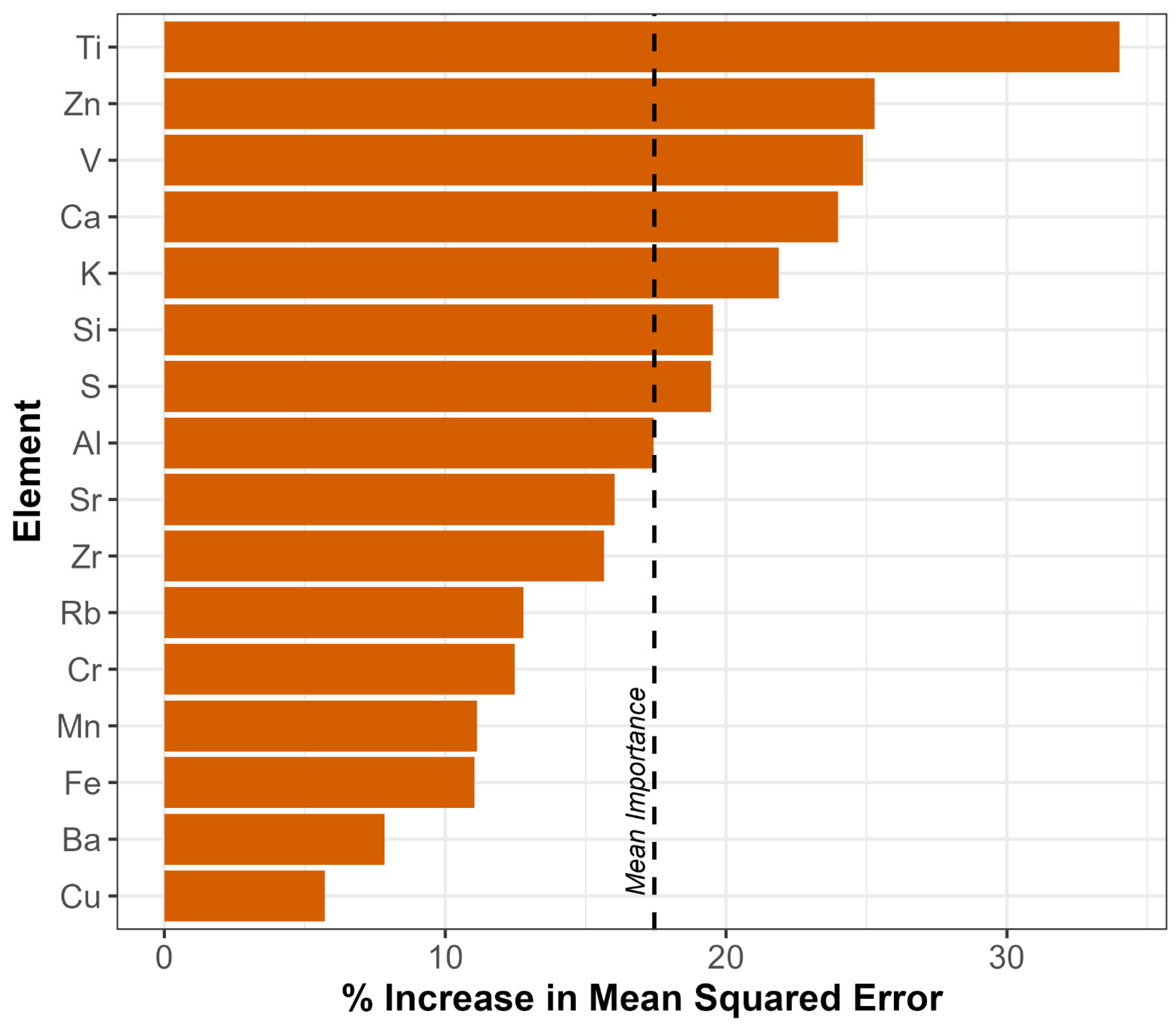
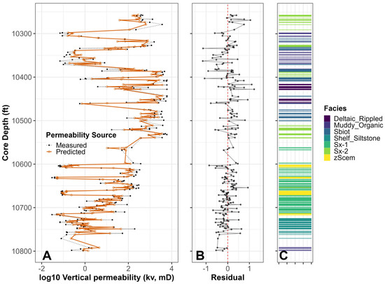
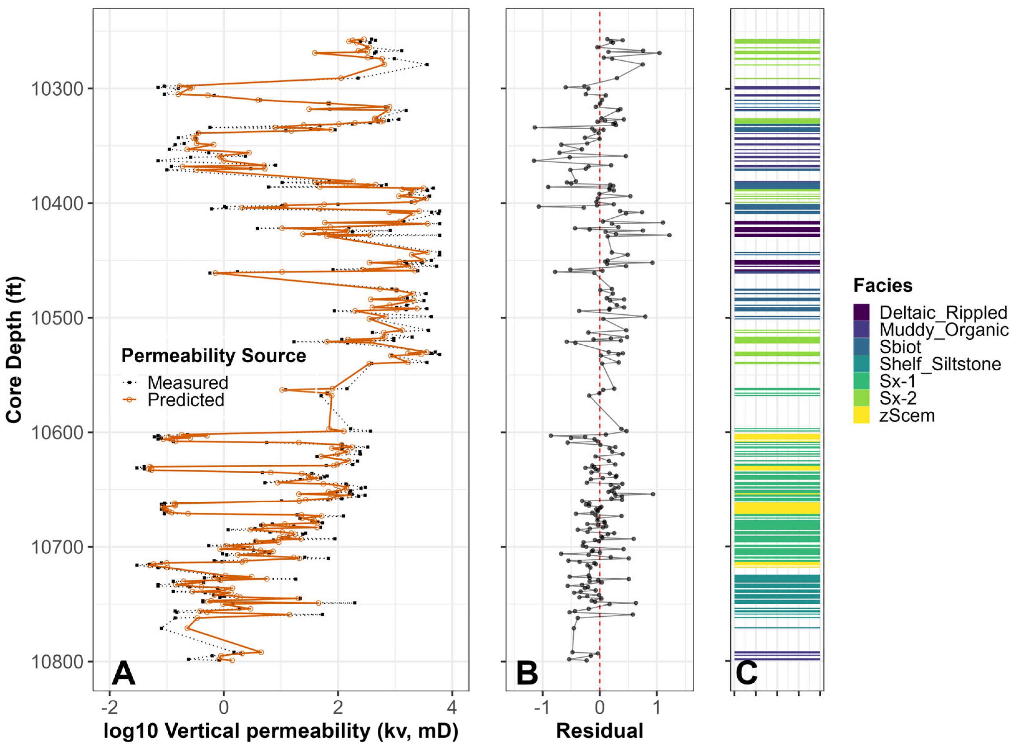
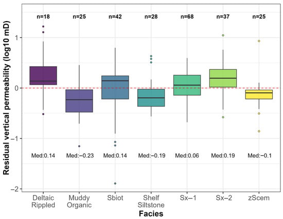
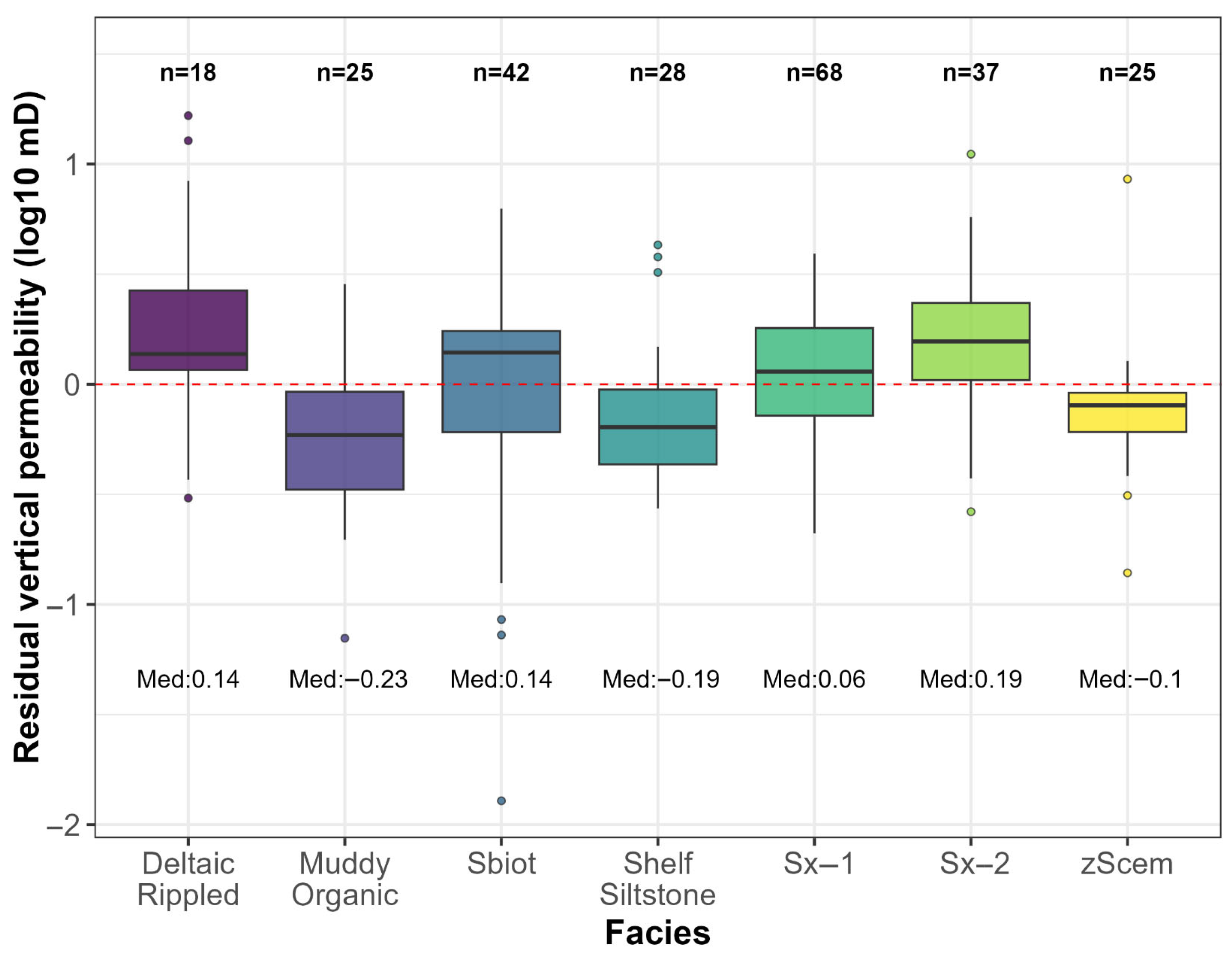
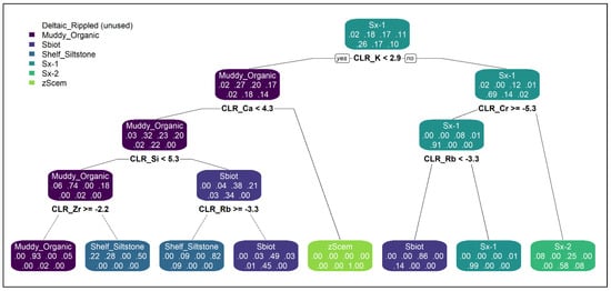
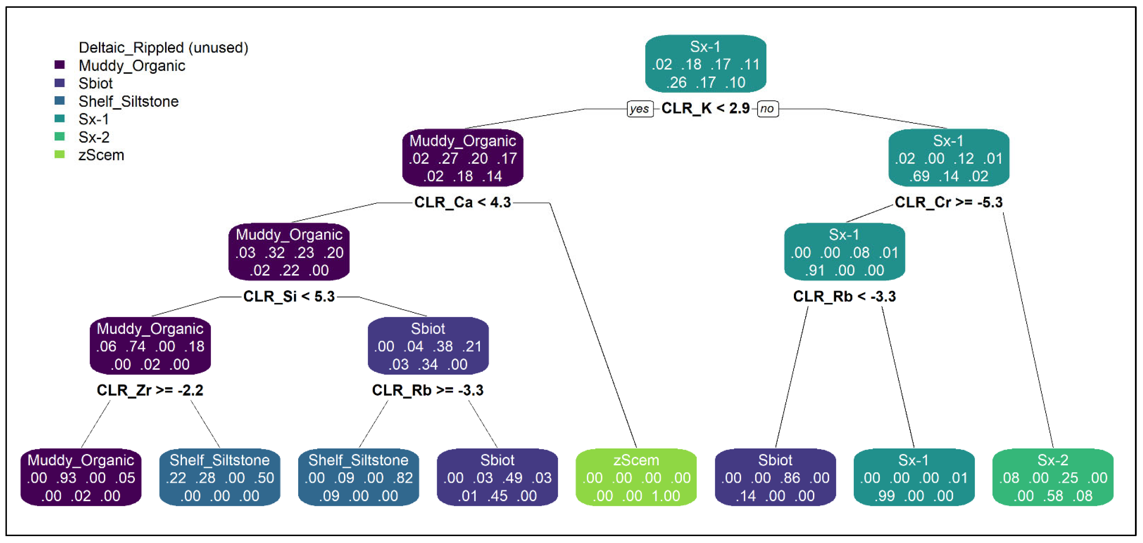
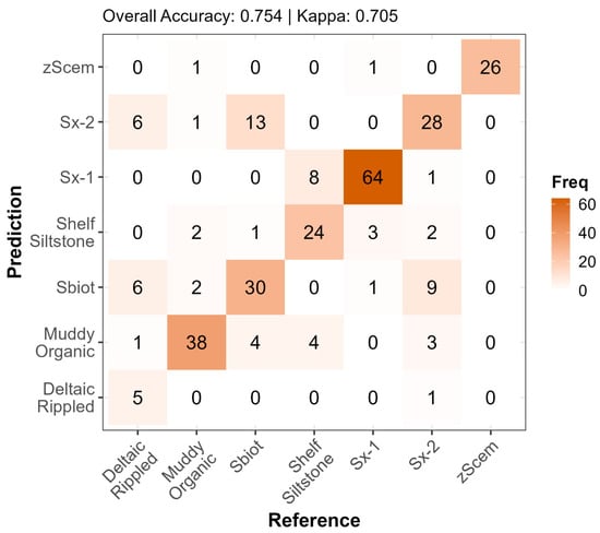
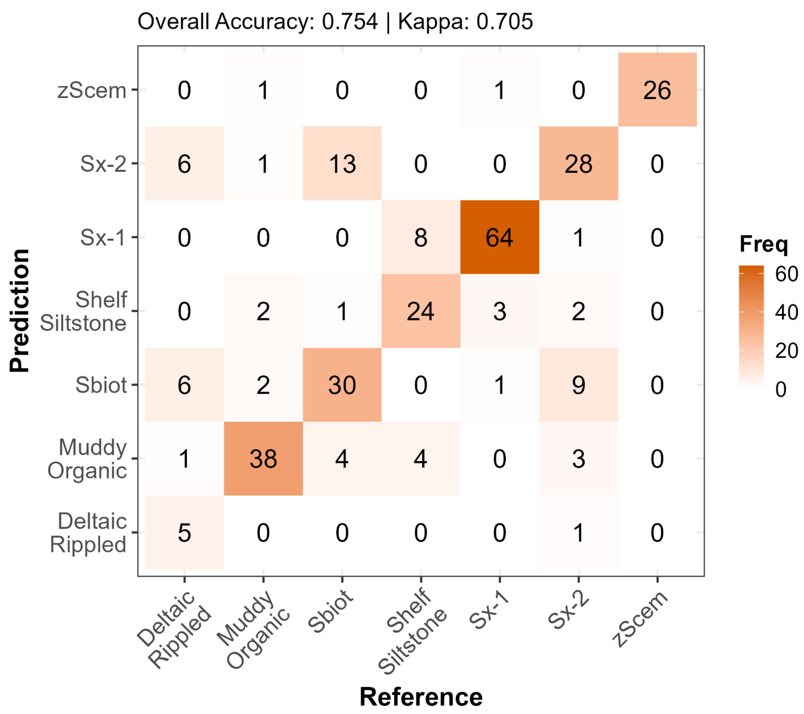
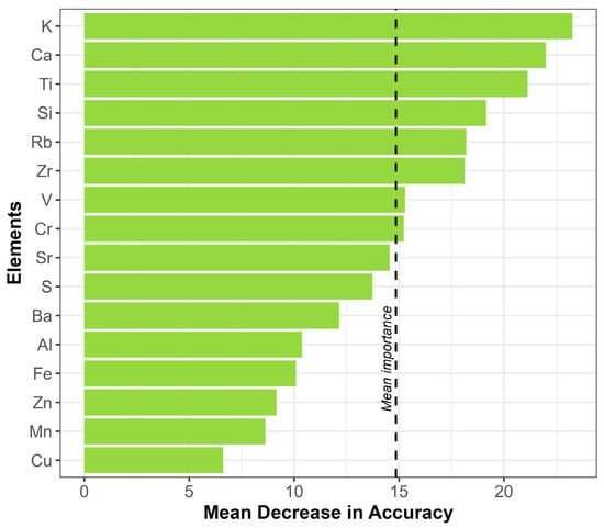
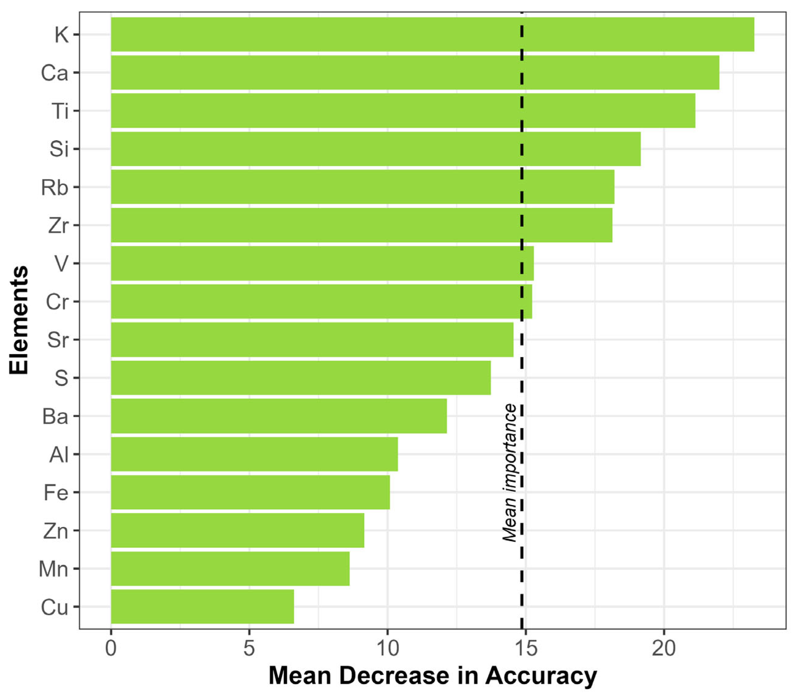

Disclaimer/Publisher’s Note: The statements, opinions and data contained in all publications are solely those of the individual author(s) and contributor(s) and not of MDPI and/or the editor(s). MDPI and/or the editor(s) disclaim responsibility for any injury to people or property resulting from any ideas, methods, instructions or products referred to in the content. |
© 2026 by the authors. Licensee MDPI, Basel, Switzerland. This article is an open access article distributed under the terms and conditions of the Creative Commons Attribution (CC BY) license.