Transport of Scomber japonicus Larvae in Different Kuroshio Paths Investigated by a Coupled Ocean–Biophysical Model

Abstract

The transport and distribution of Scomber japonicus larvae significantly affect their habitat and population dynamics. Understanding these processes is crucial for developing effective fishing and conservation strategies. However, the interannual variability of the Kuroshio path introduces both complexity and uncertainty. This study implemented a coupled ocean–biophysical model to simulate and analyze the transport of S. japonicus larvae in the Pacific Ocean south of Japan across three Kuroshio path modes, including the offshore non-large-meander (ONLM), nearshore non-large-meander (NNLM), and typical large-meander (TLM) paths. Two transport scenarios, passive drift (PD) and active swimming (AS), were considered in the simulations. The simulated results presented a comprehensive analysis of the distribution, connectivity, and transport distances of S. japonicus larvae. These findings highlighted the significant influence of biological behavior on larval transport, notably reducing transport distances and shifting the distributions northward. This allowed larvae to actively migrate to areas with higher zooplankton aggregation. Larvae released from the western and nearshore spawning grounds around Southern Kyushu–Shikoku were mainly transported to the central nursery region between 132.5° E and 140° E, whereas larvae released from the eastern spawning grounds were mainly distributed in the eastern nursery region east of 140° E near the Kuroshio Extension. These patterns suggest that nursery areas 2 and 3 may warrant further attention in future spatial management assessments, particularly when considering larval transport under different Kuroshio path modes. This study provides valuable insights into the transport and distribution mechanisms of S. japonicus larvae, offering critical guidance for the conservation of fishery resources and the promotion of sustainable fishery management.

1. Introduction

S. japonicus, a key economically important fish species in the Northwest Pacific, is primarily harvested in China, Japan, Russia, and South Korea [1,2]. The population of S. japonicus saw a significant decline in the 1980s and has been classified as overfished since the 1990s [3,4]. Despite the adoption of the Convention on the Conservation and Management of High Seas Fisheries Resources in the North Pacific Ocean in 2012 (https://www.npfc.int/ (accessed on 23 May 2026)) to address overfishing, the population has not yet recovered, owing to climate change and frequent human maritime activities [5]. Sustainable exploitation of S. japonicus is crucial, particularly during its early life stages, including egg and larval stages, which are significantly influenced by the physical marine environment in terms of survival, growth, and replenishment [6,7,8]. Since larval distribution largely determines the abundance of the species, studying the distribution of S. japonicus during its larval stage is increasingly critical [9].

S. japonicus is divided into two cohorts based on the region: the Tsushima cohort and the Pacific cohort [10]. Among these, the Pacific cohort has a higher population proportion and is influenced more by the Kuroshio current, making its habitat more vulnerable to change. Sassa and Tsukamoto (2010) [11] discovered that the intensity of the Kuroshio intrusion significantly affected the growth, transport, and distribution of S. japonicus in the East China Sea. Kamimura et al. (2015) [12] identified sea surface temperature in the Kuroshio region as a major factor affecting the growth rate and recruitment intensity of S. japonicus larvae. Kaneko et al. (2019) [13] discovered that spawning grounds closer to the Kuroshio axis result in higher spawning numbers, while greater distances led to the lower spawning numbers. Guo et al. (2022) [14] suggested that the larvae located north of the Kuroshio axis experienced a better prey environment, exhibited higher growth rates, and reached the superior feeding grounds.

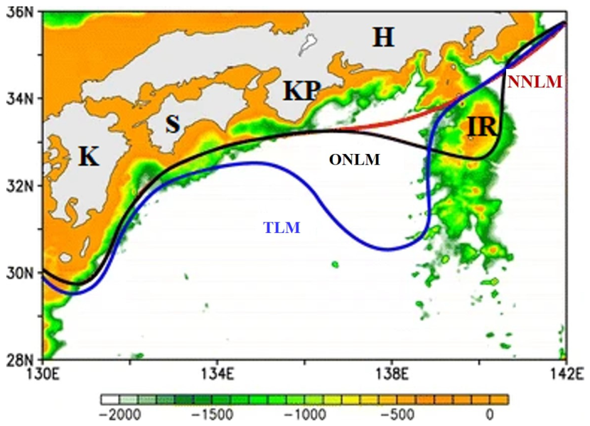
Collectively, these studies demonstrated the Kuroshio’s decisive role in the early life stages of S. japonicus. The Kuroshio exhibited the interannual variability, particularly in the Pacific Ocean south of Japan, and could be classified into three paths: the typical large-meander (TLM) path, offshore non-large-meander (ONLM) path, and nearshore non-large-meander (NNLM) path [15,16,17] (Figure 1). The shapes and physical dynamics of these paths vary considerably, which inevitably affects the larval transport and distribution [14]. To date, no comprehensive study has examined the effects of different Kuroshio paths on larval transport and distribution. Therefore, this study focused on the transport of S. japonicus larvae during the three Kuroshio path periods in the Pacific Ocean south of Japan.

Owing to observational limitations, recent studies on larval transport processes have increasingly employed the coupling of ocean models with biophysical models. Ospina-Alvarez et al. (2012) [18] integrated the biophysical model Ichthyop, a Lagrangian tool for simulating ichthyoplankton dynamics, with the hydrodynamic model MARS-3D to examine the impact of DVM (diel vertical migration) on the transport of European anchovy larvae. Huang et al. (2021) [19] combined the CROCO model with Ichthyop to investigate blue mackerel larval transport in the East China Sea. Zhou et al. (2024) [20] used the combination of CROCO and Ichthyop to investigate the dispersal and connectivity of red snapper (Lutjanus campechanus) larvae in the Northern Gulf of Mexico. These studies demonstrated that the coupled ocean–biophysical models effectively captured the effects of the physical environment and biological behavior on larval stages, providing a robust foundation for this research.

Transport research on S. japonicus larvae using the ocean model CROCO coupled with the biophysical model Ichthyop has been validated. This study focused on two main aspects of utilizing this coupled model. Physically, it examined three distinct Kuroshio paths, emphasizing the effects of currents and eddies on larval transport. Biologically, it considered three direct factors affecting larval transport: buoyancy, swimming and DVM [21,22]. Upon the aforementioned, this study systematically investigated the distribution patterns and transport distances of larvae across the three Kuroshio path periods. The influences of oceanic currents, eddies, and prey density in shaping larval transport dynamics were comprehensively examined. Based on these findings, we discuss the potential implications of larval transport patterns for future habitat and fishery management studies.

The remainder of this paper is organized as follows: Section 2 reviews the methods and materials, including the CROCO and Ichthyop models, and details the experimental setup. Section 3 presents and analyzes the simulation results of the coupled model. Section 4 discusses the key findings, placing them within the broader scientific context. Section 5 presents the conclusions.

2. Methods and Materials

2.1. Ocean Model

CROCO v2.0 (http://www.croco-ocean.org (accessed on 23 May 2026)) is an oceanic modeling system renowned for its precision and capability to capture the complex topography and dynamics of coastal areas. CROCO provides the essential hydrodynamic data, including current velocity, temperature, and salinity, for use in the biophysical model of Ichthyop.

The modeling domain spans 122–152° E and 25–45° N, encompassing the areas of the three Kuroshio paths and part of the Kuroshio Extension. The simulation periods included 2009, 2013, and 2018. The shoreline data for CROCO were sourced from the Global Self-consistent Hierarchical High-resolution Shorelines provided by the National Geophysical Data Center of the U.S. The model grid was based on the 2-Minute Gridded Global Relief Data (ETOPO2) topography [23], with a horizontal resolution of 1/12° and 32 sigma levels vertically, incorporating the stretching parameters of 5 at the surface and 0.6 at the bottom to enhance upper ocean resolution. The harmonic constants for eight tidal components (M2, S2, N2, K2, K1, O1, P1, and Q1) were obtained from the OTIS model at Oregon State University (https://www.tpxo.net/tpxo-products-and-registration (accessed on 23 May 2026)). The initial and boundary conditions were sourced from the HYCOM + NCODA Global 1/12° Reanalysis/Analysis data (https://www.hycom.org/dataserver/gofs-3pt1/analysis (accessed on 23 May 2026)), and the forcings were derived from the National Centers for Environmental Prediction Climate Forecast System Version 2 6-hourly Products (https://rda.ucar.edu (accessed on 23 May 2026)).

2.2. Biophysical Model

Ichthyop v3.3 (http://www.ichthyop.org/ (accessed on 23 May 2026)) It is a well-established model used to study the effects of physical and biological factors on ichthyoplankton dynamics [24]. It incorporates the essential processes in the early life stages of fish, such as spawning, swimming, and buoyancy. The time series data of velocity, temperature, and salinity fields from ocean models were adopted as the input in Ichthyop to simulate the physical environment.

2.2.1. Habitat of S. japonicus

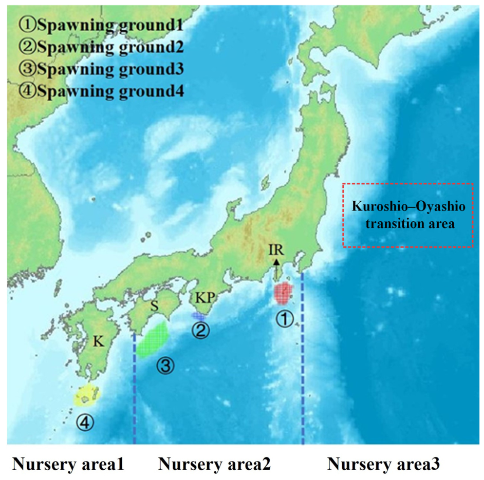
Japanese fisheries have identified four spawning grounds in the Pacific Ocean south of Japan [25] that were set at the same locations in Ichthyop (Figure 2). To quantitatively analyze the larval transport process, the study region was divided into three nursery areas based on Kuroshio path characteristics: nursery area 1, positioned west of 132.5° E, where the Kuroshio exhibited the coastal characteristics and tended to carry the larvae towards the shore; nursery area 2, situated between 132.5° E and 140° E, where the Kuroshio path exhibited the significant variations; and nursery area 3, located east of 140° E in the Kuroshio Extension region, is an important area for many small pelagic fish due to its high prey abundance [26]. Japanese fishery surveys have reported major spawning-related areas of the Pacific cohort of S. japonicus along the southern coast of Japan [25]. Based on these fishery records and the spatial pattern shown in Figure 2, four representative release locations were defined in the Ichthyop experiments. These spawning grounds were used as representative release locations in the Ichthyop experiments rather than as fixed spawning habitat polygons with precise latitude–longitude boundaries. Geographically, spawning ground 1 is located near the Izu Ridge, spawning ground 2 south of the Kii Peninsula, spawning ground 3 south of Shikoku, and spawning ground 4 south of Kyushu, as illustrated in Figure 2.

2.2.2. Parameter Settings

S. japonicus are positively buoyant in the egg stage. To determine the buoyancy velocity of S. japonicus eggs, this research replaced the default equation in Ichthyop, which is commonly applied to elliptical fish eggs (e.g., Engraulis capensis eggs), as S. japonicus eggs are spherical in shape. The formula employed is as follows:

$$V_b=d^2\times g\times {\displaystyle \frac{{\rho }_s-{\rho }_f}{18\mu }}$$

(1)

where $V_b$ is the buoyant velocity (cm/s), $d$ is the fish egg diameter (mm), $g$ is the gravitational force (cm/${\mathrm{s}}^2$). ${\rho }_s$ and ${\rho }_f$ represent the densities of the sea water and the fish egg, respectively (g/cm³), and $\mu$ is the water molecular viscosity (WMV, g·cm⁻¹·s⁻¹) depending on the sea temperature. A value of 1.0 mm and 0.004 g/cm³ were assigned to $d$ and the fish egg density, based on the previous studies reported by Jung et al. (2013) [27]. The density of water is variable and is obtained from the ocean model.

S. japonicus larvae develop weak swimming ability after 3 days post-hatching [28]. To simulate this behavior, two key factors of swimming direction and speed must be considered. Therefore, this research replaced Ichthyop’s default orientation option, wherein the larvae are programmed to swim in random directions, with a setting that directs the larvae to swim toward areas with higher plankton aggregation. For swimming speed, this research depended on the actual swimming situation and set it to the minimum swimming speed of 32 cm/s [29]. The larvae exhibit a diurnal cycle in specific gravity, peaking during the day and reaching its lowest point at midnight after 2–4 days after hatching [30]. It was considered a highly efficient behavioral mechanism that can significantly impact larval transport [21]. On this basis, this research set the particles (larvae) to drift passively with the current from release and to access DVM behavior after 3 days. Therefore, the particles were programmed to exhibit vertical movement, descending into deeper waters during the daytime (06:59 AM to 7:00 PM) and ascending to shallower waters during the nighttime (7:01 PM to 7:00 AM).

The time step ($dt$) for Ichthyop was set to 300 s to satisfy the Courant–Friedrichs–Lewy (CFL) criterion, which was essential for convergence in solving certain partial differential equations:

$${\displaystyle \frac{U\ast dt}{dX}}<1$$

(2)

where $U$ is the current velocity from the hydrodynamic model (CROCO), and $dX$ is the resolution of the hydrodynamic model grid. For the advection process, a fourth-order Runge–Kutta numerical scheme was employed to accurately model particle trajectories near physical obstacles such as islands and reefs [31]. To prevent the particles from moving inland and distorting the simulation results, the coastline behavior was set to bouncing, ensuring that particles rebound upon encountering the coastline [32]. Spawning grounds were positioned as described in Section 2.2.1. As S. japonicus typically spawns at depths of 0–25 m [9,33], the release depths were set between 0 and 25 m with particles evenly distributed within this range to ensure uniform distribution [24]. The parameter settings are detailed in

Table 1. Ichthyop parameter settings.

Variable	Value and Notes
Time step	300 s, satisfy the CFL criteria
Release depth	Evenly released between 0 and 25 m
Buoyant velocity	$V_b,$ Formula (1)
Spawning grounds	Demonstrated in Figure 2
Speed and direction	32 cm/s, toward to high plankton aggregation
Number of particles	4000
Coastline behavior	Bouncing
Numerical scheme of vertical process	DVM
Numerical scheme of advection process	Runge–Kutta 4

.

2.2.3. Chlorophyll-a Data

Chlorophyll-a data were used to describe the spatial pattern of phytoplankton biomass and potential lower-trophic productivity in the study region. The data were obtained from the Copernicus Marine Service NEMO biogeochemical reanalysis product (GLOBAL_MULTIYEAR_BGC_001_029; https://data.marine.copernicus.eu/product/GLOBAL_MULTIYEAR_BGC_001_029/ (accessed on 23 May 2026)). Monthly mean chlorophyll-a mass concentration in sea water was extracted for April 2009, April 2013, and April 2018, corresponding to the three particle-tracking simulation periods. Because direct zooplankton prey fields were not available for the selected years and region, chlorophyll-a was used only as an indirect proxy for potentially favorable feeding conditions and should not be interpreted as measured zooplankton abundance.

2.3. Design of Numerical Experiments

2.3.1. Transport Scenarios

Two transport scenarios were considered: PD (passive drift) and AS (active swimming). For the PD scenario, due to their weak swimming ability, it was assumed that the movement of larvae relies entirely on currents [34]. For the AS scenario, the larvae possess all biological capabilities described in the previous section, Ichthyop parameter settings (Table 1). By comparing the two transport scenarios described above, we explore the effects of biological behavior on larval transport processes.

2.3.2. Selection of the Simulation Periods

Three distinct periods characterized by significant variations in the Kuroshio path were selected: 2009, 2013, and 2018, corresponding to the ONLM, NNLM, and TLM path periods, respectively. April, identified as the peak spawning month in previous research [12,14], was selected as the experimental month. Therefore, this research set the release of 200 particles per day at each spawning ground throughout April. Given that the larval stage of S. japonicus can last 29 d or less [11], the transport duration was set to 20 d. The release time for all particles was set to 22:00 on each day after the simulation began, reflecting the typical spawning time of S. japonicus [9,33].

In total, 6 experiments were conducted (three Kuroshio paths × two transport scenarios) to examine the effects of different Kuroshio paths on larval transport and distribution. A summary of these experiments is presented in

Table 2. Design of experiments.

Path Type	Transport Scenarios	Release Locations	Release Time (22:00)	Release Number
ONLM	PD/AS	Spawning ground 1	Each day in April 2009	200
		Spawning ground 2		200
		Spawning ground 3		200
		Spawning ground 4		200
NNLM	PD/AS	Spawning ground 1	Each day in April 2013	200
		Spawning ground 2		200
		Spawning ground 3		200
		Spawning ground 4		200
TLM	PD/AS	Spawning ground 1	Each day in April 2018	200
		Spawning ground 2		200
		Spawning ground 3		200
		Spawning ground 4		200

.

2.4. Model Evaluation and Connectivity Metrics

The MD was calculated as the average difference between paired observed and simulated values using the following formula:

$$\mathrm{M}\mathrm{D}={\displaystyle \frac{1}{n}}{\sum }_{i=1}^n(O_i-S_i)$$

(3)

where $n$ is the number of observations, $O_i$ is the observed value, and $S_i$ is the simulated value.

The correlation coefficient (R) measures the strength and direction of the linear relationship between observed and simulated values. The formula for the correlation coefficient (R) is

$$R^2={\left({\displaystyle \frac{{\sum }_{i=1}^n\left(O_i-\overline{O}\right)\left(S_i-\overline{S}\right)}{\sqrt{{{\sum }_{i=1}^n\left(O_i-\overline{O}\right)}^2}\sqrt{{{\sum }_{i=1}^n\left(S_i-\overline{S}\right)}^2}}}\right)}^2$$

(4)

where $\overline{O}$ is the mean of the observed values, and $\overline{S}$ is the mean of the simulated values. Moreover, $R^2$ ranges from 0 to 1, where 0 indicates no correlation and 1 indicates perfect correlation.

The connectivity between the spawning grounds and nursery areas was calculated as follows:

$$p_{ij}={\displaystyle \frac{n_{ij}^{\prime }}{n_i}}$$

(5)

where $p_{ij}$ represents the connectivity between $i$-th spawning ground and $j$-th nursery area; $n_i$ is the number of particles released in the $i$-th spawning ground; and $n_{ij}^{\prime }$ is the number of particles remaining in the $j$-th nursery area after the simulation.

3. Results

3.1. Model Validations

3.1.1. Currents

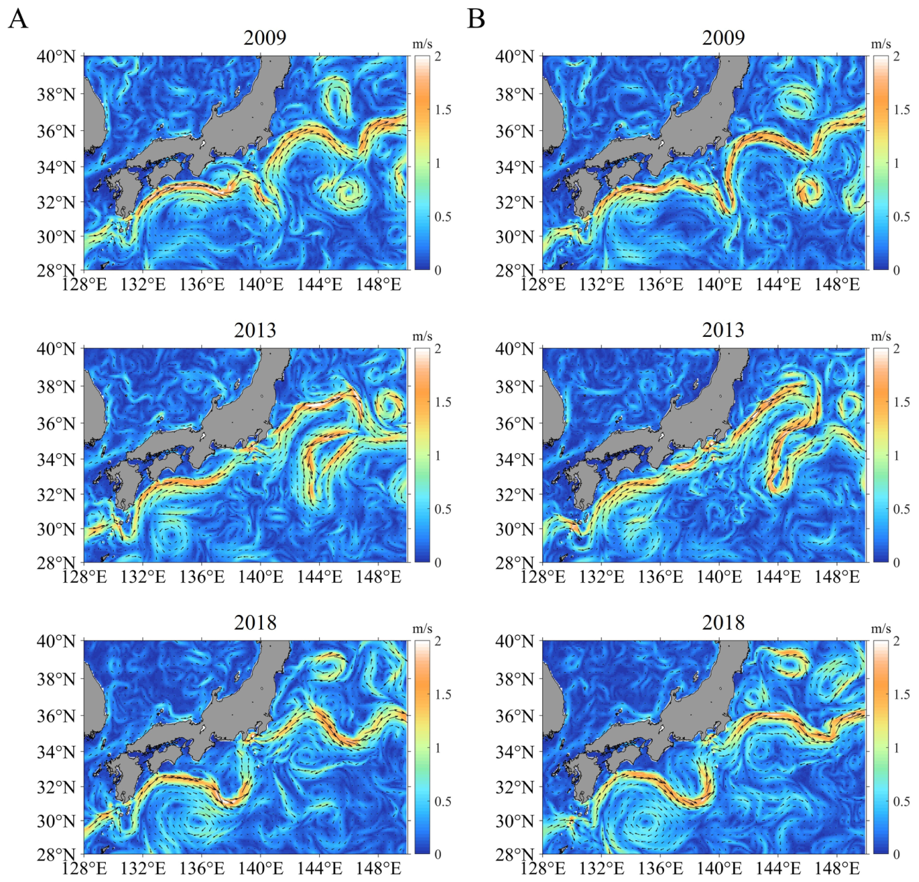
The Kuroshio, as a western boundary current, exhibits significantly higher speeds compared to the surrounding waters. Within the core of the Kuroshio, speeds can exceed 2 m/s, while those in the surrounding areas typically range from 0.1 m/s to 0.5 m/s. Accurate simulation of current is critical to the Ichthyop model, as it directly impacts the transport and distribution processes within the system. To validate the simulated current fields, this research compared the monthly average currents of the model with the HYCOM + NCODA global 1/12° reanalysis data (https://hycom.org/data/ (accessed on 23 May 2026)) for April 2009, 2013, and 2018. The comparison results are shown in Figure 3; the shapes and velocities of the Kuroshio during the three path periods were well-simulated, with the main axis and its meander accurately captured, indicating that the model effectively reproduced the key features of the Kuroshio.

3.1.2. Tides

The harmonic constants were utilized to validate the model at various tide stations with data obtained from the University of Hawaii Sea Level Center [35]. The analysis focused on the harmonic constants of four major tidal components: M2, S2, K1, and O1. Tidal heights and phase angles were compared across 12 selected stations, as shown in

Table 3. Name and location of tidal stations.

No	Station Name	Longitude (° E)	Latitude (° N)
1	Aburatsu	131.417	31.567
2	Hakodate	140.733	41.783
3	Kushimoto	135.783	33.467
4	Kushiro	144.383	42.967
5	Mera	139.833	34.917
6	Miyakejima	139.482	34.067
7	Naha	127.667	26.217
8	Naze	129.495	28.382
9	Nishinoomote	130.992	30.735
10	Ofunato	141.75	39.017
11	Toyama	137.217	36.767

.

Table 4. Statistical analysis compared model-simulated and observed harmonic constants for M2, S2, K1, and O1 at 12 stations during April 2009, 2013, and 2018.

Time	Tidal Constituents	Amplitude Mean Differences/cm	Amplitude Correlation Coefficient (R2)	Phase-Lag Mean Differences/°	Phase-Lag Correlation Coefficient (R2)
2009	M2	1.7	0.9874	3.7	0.9935
	S2	1.7	0.9902	2.5	0.9976
	K1	2.5	0.9720	2.4	0.9895
	O1	1.9	0.9833	4.1	0.9822
2013	M2	1.5	0.9897	2.9	0.9812
	S2	1.8	0.9826	1.8	0.9963
	K1	2.4	0.9799	3.3	0.9824
	O1	1.1	0.9923	3.6	0.9913
2018	M2	1.9	0.9974	4.4	0.9966
	S2	1.5	0.9781	3.9	0.9982
	K1	2.2	0.9230	3.2	0.9968
	O1	2.1	0.9536	4.2	0.9851

presents the mean differences (MDs) and correlation coefficients ($R^2$) between the simulated and observed harmonic constants for the four main tidal constituents. For the specific calculation formula, please refer to Section 2.4.

The maximum difference in amplitude did not exceed 2.5 cm, and the maximum difference in phase lag did not exceed 4.4°, indicating a strong agreement between the simulated and observed tide amplitudes and phase angles. Although minor deviations were present across the three periods, they remained within the normal range.

3.1.3. Temperature

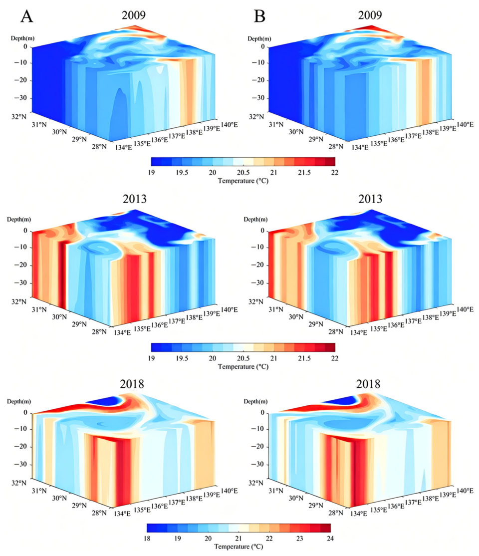
The hatching rate of eggs, larval growth, and survival are all closely linked to upper ocean water temperatures. Therefore, ensuring the accuracy of model simulations for upper-layer water temperatures is crucial. To validate the modeling temperature, this research selected a portion of the modeled region in April (134° E–140° E, 28° N–32° N), coinciding with the location where the Kuroshio current bends. The results are presented in Figure 4, showing the annual variability and the comparison with reanalysis data from the Nucleus for European Modeling of the Ocean (NEMO, downloaded from CMEMS). It is shown that upper-layer temperatures were lower in 2009 and higher in 2013 and 2018. Additionally, the temperature of the Kuroshio current was consistently higher than that of the surrounding sea during these periods. It is indicated that the model is capable of reproducing the prominent features of the upper-layer water temperatures.

3.2. Larval Distributions

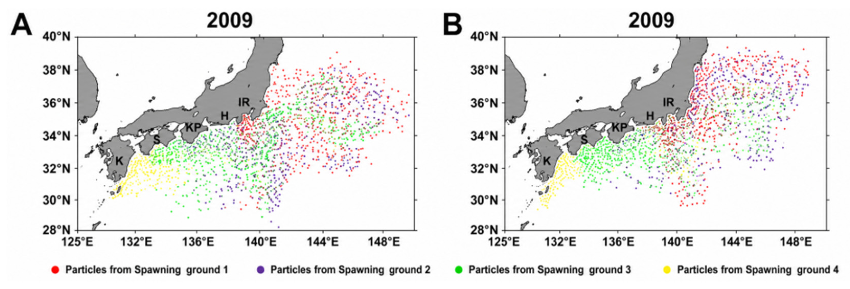
Here, this research presents the results of a 20-day simulation of larvae distribution. During the ONLM period, the Kuroshio path is relatively stable, with small oscillations and small meander. In the PD scenario (Figure 5A), larvae from spawning grounds 1 and 2 (red and purple particles) were transported eastward following the Kuroshio current, leading to significant offshore dispersal into the central Pacific. Some of these larvae were also influenced by a southward-branching tributary of the Kuroshio at ~140° E. The larvae from spawning grounds 3 and 4 (green and yellow particles) exhibited higher nearshore retention, forming clusters near Southern Kyushu and Shikoku. Meanwhile, some larvae were influenced by the anticyclonic eddy south of Shikoku Island, resulting in an entrapment within the eddy, preventing the further eastward movement. Conversely, in the AS scenario (Figure 5B), biological behaviors enhanced nearshore retention. Larvae from all spawning grounds exhibited reduced offshore dispersal, forming notable aggregations near Kyushu, Shikoku, Kii Peninsula, and the Izu Ridge. However, a significant number of larvae were still observed far from the shore south of Shikoku Island and near 140° E.

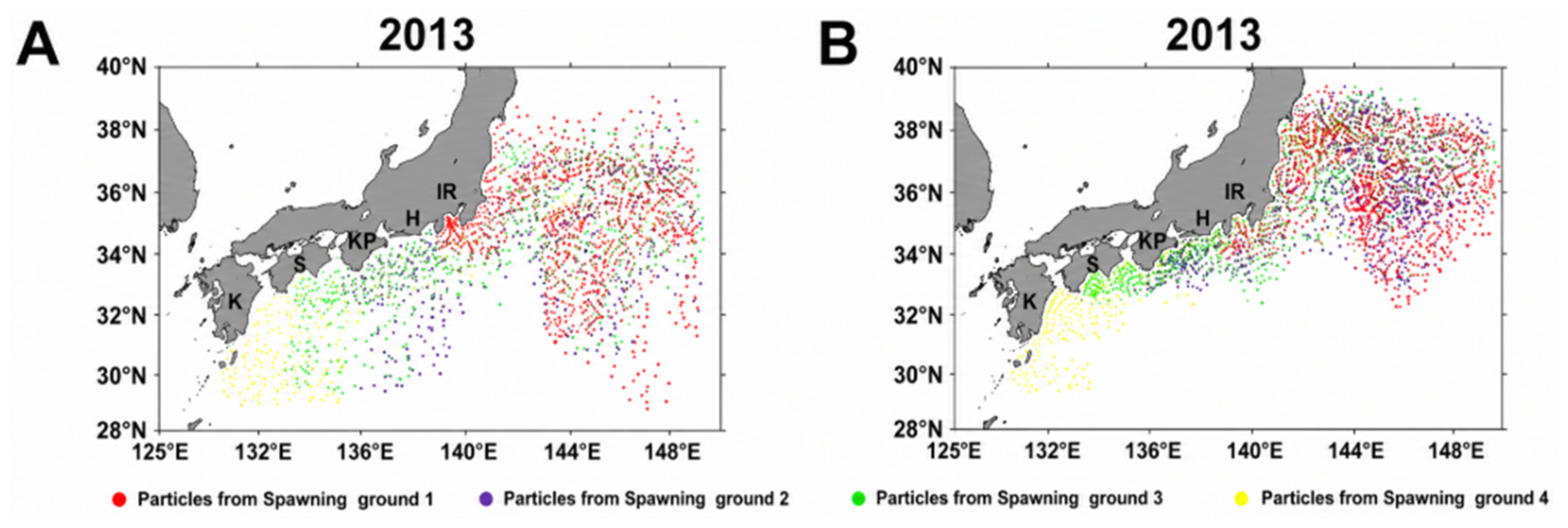
Compared to the ONLM, the main path of the Kuroshio during the NNLM is closer to the Japanese coastline, particularly near Southern Shikoku and Honshu. It is characterized by faster current speeds, a relatively stable flow direction, and greater interaction with the continental shelf. In the PD scenario (Figure 6A), larvae from spawning grounds 1 and 2 experienced accelerated northeastward dispersal, with a significant portion reaching the Central Pacific. However, due to the proximity of the Kuroshio CurrentKuroshio current to the shore, the complex coastal environment caused some larvae to being be retained between Honshu Island and the Izu Ridge. Larvae from spawning grounds 3 and 4 exhibited a wider spatial distribution, with fewer larvae remaining nearshore. In the AS scenario (Figure 6B), larvae from all spawning grounds exhibited a tendency to aggregate near the coast.

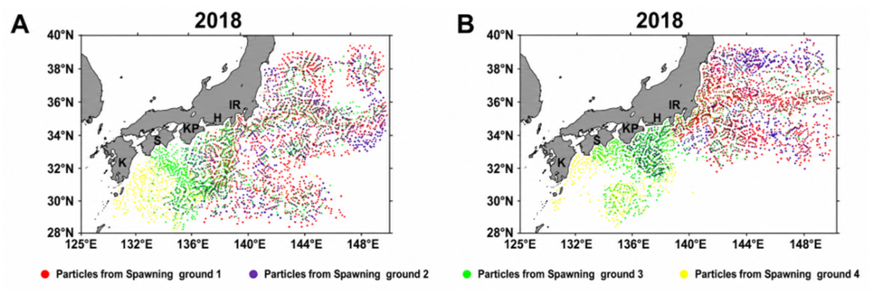
The Kuroshio during the TLM is characterized by its pronounced large-meander pattern, featuring a path that shifts away from the coastline, significant variations in current velocity, and actively mesoscale eddy. In the PD scenario (Figure 7A), the larval distribution was the most extensive among the three modes. Larvae from spawning grounds 1 and 2, while being transported eastward by the Kuroshio current, were also influenced by the southeastward branch near 140° E and the anticyclonic eddies on both sides of the main Kuroshio flow between 141° E and 148° E. These factors lead to a distribution range spanning from 28° N to 39° N. In the AS scenario (Figure 7B), biological behaviors enhanced nearshore retention, particularly for larvae from spawning grounds 3 and 4, which showed significant aggregation near Kyushu and Shikoku. However, a considerable number of larvae were still retained south of the Kii Peninsula. Meanwhile, larvae from spawning grounds 1 and 2, guided by biological behaviors, followed the Kuroshio current and migrated directly to the Kuroshio–Oyashio transition area.

3.3. Transport Distance

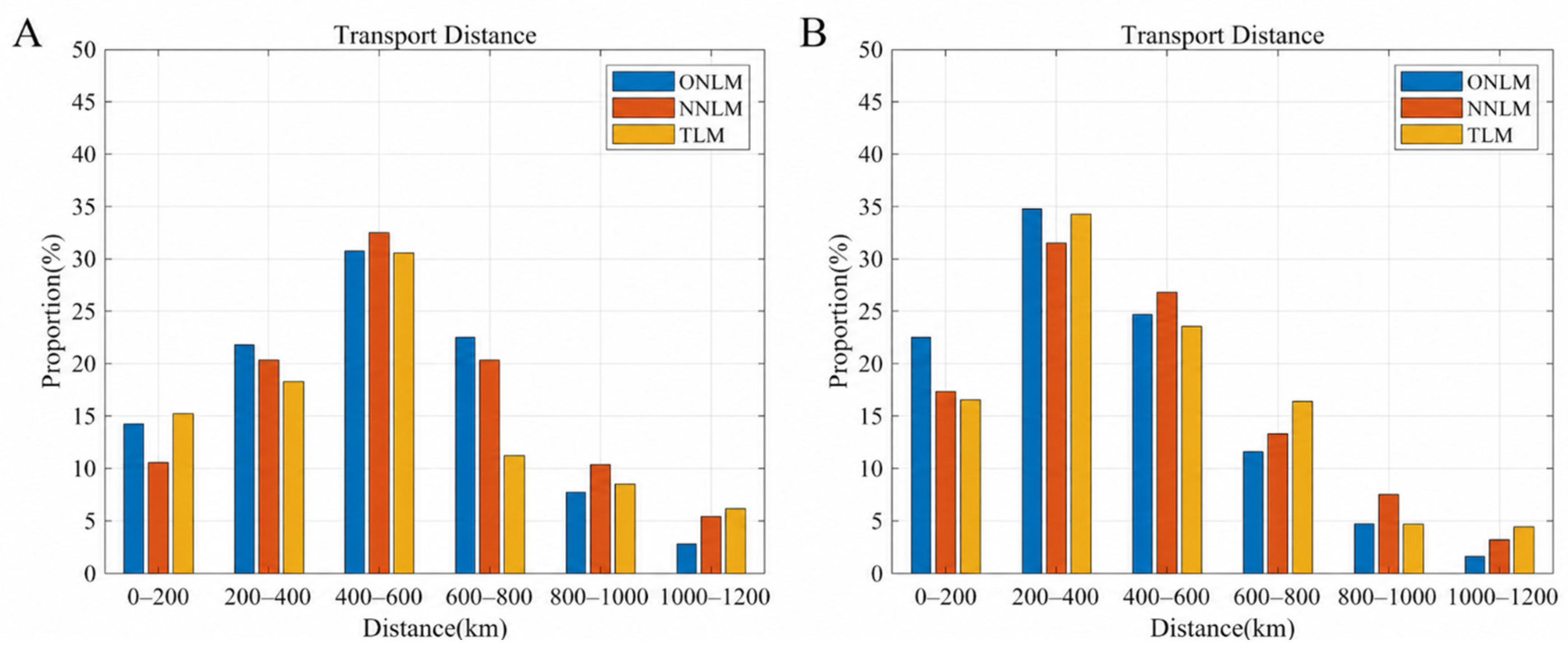
The larval transport distances across the three periods were systematically analyzed with two transport scenarios (Figure 8). In the PD scenario (Figure 8A), larval dispersal is predominantly governed by ocean currents, resulting in a broader spatial distribution. The highest proportion (30–35%) of larvae is transported for mid-distances (400–600 km), reflecting the significant influence of the Kuroshio current. Short-distance transport (0–400 km) accounts for a relatively smaller proportion due to the absence of active retention mechanisms, while approximately 15–20% of larvae are transported over long distances (600–1200 km), driven by the strong Kuroshio current and its southward branching near 140° E.

In contrast, the AS scenario (Figure 8B) demonstrates the critical role of biological behavior in enhancing nearshore retention. Nearshore waters, characterized by weaker ocean currents, eddies, and tidal movements, along with complex coastal topography such as bays, islands, and coral reefs, provide favorable conditions for larval aggregation. These features create hydrodynamic convergence zones, which offer larvae with suitable habitats and shield them from the disruptive effects of strong offshore currents. Consequently, the proportion of larvae within short distances (0–400 km) increases significantly, surpassing 25% in all periods. Mid-distance transport (400–600 km) slightly declines compared to the PD scenario, while long-distance transport (600–1200 km) drops substantially, with very few larvae reaching beyond 800 km. This pattern highlights the influence of biological behavior in concentrating larvae within ecologically favorable nearshore zones.

3.4. Connectivity

To better quantify the larval distribution and facilitate the jurisdictional management, the connectivity was introduced [36,37]. For the specific calculation, refer to Equation (5) in Section 2.4.

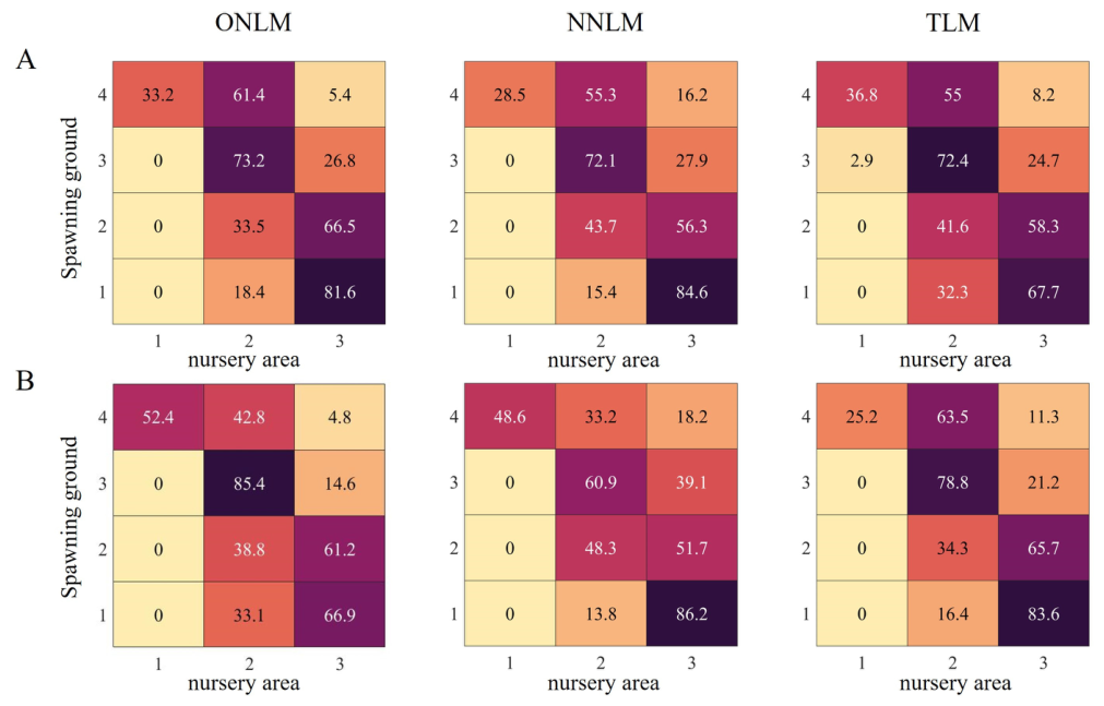
Figure 9 illustrates the larval connectivity in both PD and AS transport scenarios. During all three periods, larvae from spawning grounds 3 and 4 show higher connectivity with nursery area 2, whereas larvae from spawning grounds 1 and 2 exhibit stronger connectivity with nursery area 3. This indicates that nursery areas 2 and 3 serve as the primary habitat at the end of the simulation.

4. Discussions

4.1. Different Transport Scenarios

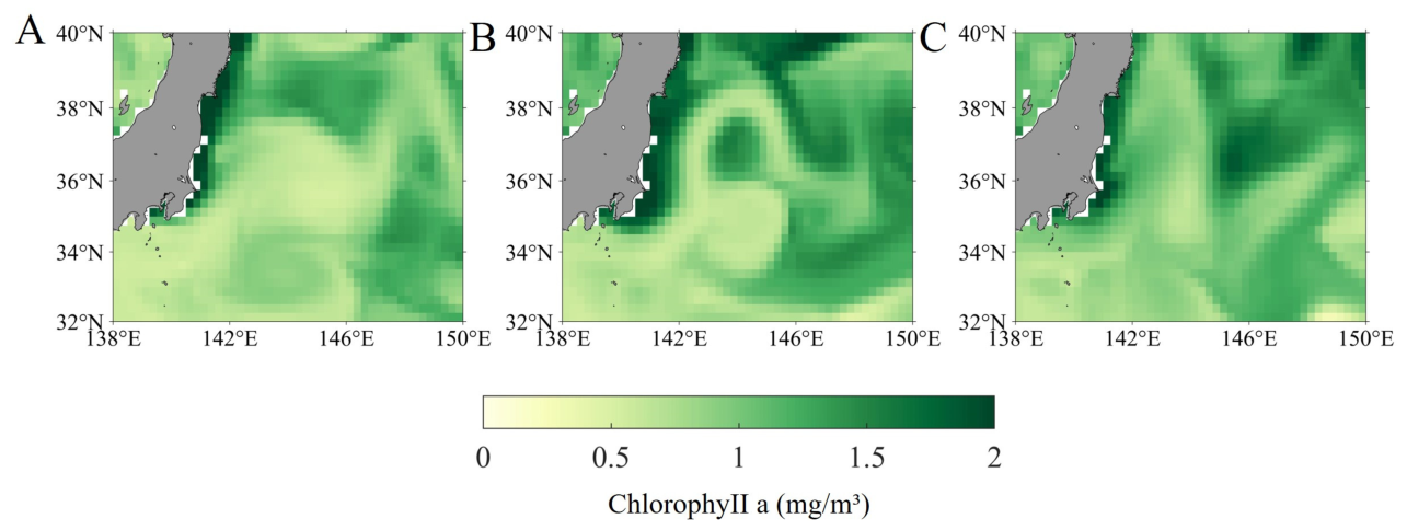
Under the AS transport scenarios, the Kuroshio current carried a substantial number of larvae into the Kuroshio–Oyashio transition area, located between 143° E and 147° E (Figure 5, Figure 6 and Figure 7). In this region, the convergence of the warm Kuroshio and the cold Oyashio currents generated upwelling processes that transported nutrient-rich deep waters to the surface. These upwelling dynamics markedly enhanced the productivity of phytoplankton and zooplankton, thereby supplying abundant food resources critical for larval growth and survival. As shown in the chlorophyll-a distribution (Figure 10), the larvae exhibited behavioral adaptations that enabled them to seek out favorable environmental conditions.

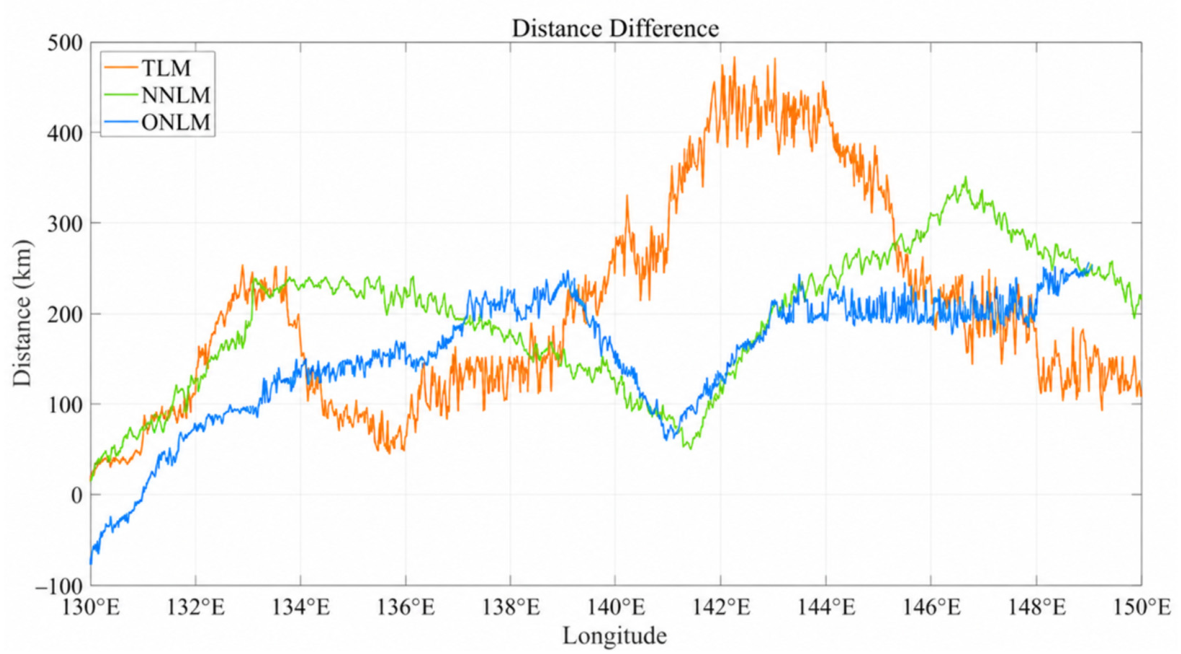
Consequently, the larvae tended to aggregate in regions with higher chlorophyll-a concentrations compared to those in the PD scenarios, particularly within the Kuroshio–Oyashio Transition Zone and coastal areas. This behavioral preference resulted in a northward shift in larval distribution under the AS scenarios. To quantitatively assess this northward movement, this research calculated the difference in the mean latitude of larvae between scenarios, as illustrated in Figure 11. The largest difference is observed during the TLM period, where the maximum northward shift is 473.2 km, occurring between 142° E and 144° E. This significant difference is due to the complex meandering of the Kuroshio current, which drove a portion of the PD scenario larvae southward, while larvae in the AS scenario, actively migrated toward areas with higher prey density, such as the Kuroshio–Oyashio transition area. Additionally, smaller peaks can also be observed in both the ONLM and NNLM periods, especially in the longitudinal ranges of 132° E–134° E. These peaks indicate that larvae in the AS scenario consistently exhibited a preference for productive nearshore waters, resulting in higher retention rates along the coast.

4.2. Potential Implications for Spatial Management

Nursery area 2 is a critical zone characterized by pronounced Kuroshio meandering, active eddy dynamics, and expansive nearshore waters. While some larvae successfully establish suitable habitats along the coastline, many others in this region face significant survival challenges due to the complex hydrodynamic conditions. These challenges include increased predation pressure, limited food availability, and harsh environmental conditions. The high connectivity and retention in nursery area 2 suggest that this region may deserve further attention in future spatial management assessments. However, the present model does not explicitly simulate predation, habitat quality, or protection effects. Therefore, any potential application of dynamic MPAs in this region should be regarded as a management hypothesis that requires additional ecological and fishery evidence.

Nursery area 3 showed strong endpoint connectivity and was located near productive waters associated with the Kuroshio–Oyashio transition region. These results indicate that this area may be important for larval transport and potential nursery function. However, the present model does not evaluate fishing pressure, pollution exposure, seagrass beds, coral reefs, or other habitat-quality variables. Therefore, specific conservation actions in this area should be evaluated in future studies by combining larval transport simulations with habitat surveys, fishery data, and long-term ecological monitoring.

Future studies should further integrate larval transport simulations with observations of habitat quality, prey availability, mortality, fishing activity, and environmental stressors. Such integrated analyses would be necessary before proposing specific conservation measures for nursery areas 2 and 3.

4.3. Limitations and Future Work

Several limitations should be noted when interpreting the present results. First, the hydrodynamic forcing and boundary conditions may influence the simulated larval trajectories. Although the CROCO model reproduced the main Kuroshio structures used in this study, the comparison with HYCOM + NCODA should be interpreted mainly as a consistency assessment because HYCOM + NCODA also provided the initial and boundary conditions. Second, the biological behavior of larvae was simplified in the particle-tracking experiments. The PD scenario represents a passive-dispersal baseline, whereas the AS scenario represents an idealized active-swimming case. These scenarios do not fully resolve stage-specific processes such as egg buoyancy changes, hatching time, the onset of diel vertical migration, and the developmental timing of active orientation. Third, the prescribed swimming speed and prey-seeking behavior introduce additional uncertainty. The swimming speed used in the AS scenario may overestimate the ability of early-stage larvae, and a lower, ontogeny-dependent swimming speed scheme would be more realistic. In addition, chlorophyll-a was used only as an indirect proxy for potentially favorable feeding conditions. It reflects phytoplankton biomass and lower-trophic productivity, but it does not directly represent zooplankton prey abundance. Fourth, larval mortality was treated in a simplified way and did not explicitly include predation, starvation, fishing pressure, pollution exposure, or habitat-quality effects. Finally, each Kuroshio path mode was represented by a single case year. Therefore, the results should be interpreted as case-based comparisons under different Kuroshio path backgrounds rather than as long-term mean responses of each path mode. Future studies should incorporate multiple years for each path type, independent observational validation, stage-dependent larval behavior, direct prey fields, survival functions, and uncertainty estimates to provide a more comprehensive assessment of larval transport and connectivity.

5. Conclusions

This study used a coupled CROCO–Ichthyop model to examine the transport of S. japonicus larvae under three Kuroshio path conditions and two transport scenarios. The results show that larval distribution was strongly shaped by both the Kuroshio path and biological behavior. Compared with passive drift, active swimming shifted larval distributions northward and reduced transport distances, with most larvae transported over shorter ranges of approximately 200–400 km.

Among the three Kuroshio path conditions, the typical large-meander case produced the widest larval distribution because of the pronounced meandering flow and associated eddy activity, whereas the nearshore non-large-meander case led to a narrower distribution under a more stable Kuroshio path. Connectivity analysis further indicated that larvae released from Southern Kyushu and Shikoku were mainly transported to the central region between 132.5° E and 140° E, while larvae released from the waters south of the Kii Peninsula and near the Izu Ridge were more frequently distributed east of 140° E near the Kuroshio Extension and the Kuroshio–Oyashio transition region.

These findings suggest that changes in Kuroshio path configuration can alter larval dispersal pathways and potential nursery connectivity. The results should be interpreted as case-based transport patterns under selected Kuroshio path conditions, and future work should further incorporate multi-year simulations, stage-dependent larval behavior, direct prey fields, and independent observational validation.

References

1. Hiyama, Y.; Yoda, M.; Ohshimo, S. Stock size fluctuations in chub mackerel (Scomber japonicus) in the East China Sea and the Japan/East Sea. Fish. Oceanogr. 2002, 11, 347–353. [Google Scholar] [CrossRef]
2. Yukami, R.; Ohshimo, S.; Yoda, M.; Hiyama, Y. Estimation of the spawning grounds of chub mackerel Scomber japonicus and spotted mackerel Scomber australasicus in the East China Sea based on catch statistics and biometric data. Fish. Sci. 2009, 75, 167–174. [Google Scholar]
3. Crone, P.R.; Hill, K.T.; Zwolinski, J.P.; Kinney, M.J. Pacific Mackerel (Scomber japonicus) Stock Assessment for US Management in the 2019-20 and 2020-21 Fishing Years; Pacific Fishery Management Council: Portland, Oregon, 2019; 112p. [Google Scholar]
4. Yukami, R.; Nishijima, S.; Isu, S.; Kamimura, Y.; Furuichi, S.; Watanabe, R. Stock assessment and evaluation for the Pacific stock of chub mackerel (fiscal year 2018). In Marine Fisheries Stock Assessment and Evaluation for Japanese Waters (Fiscal Year 2018/2019); Fisheries Agency and Fisheries Research Agency of Japan: Tokyo, Japan, 2019; pp. 163–208. [Google Scholar]
5. Hong, J.B.; Kim, D.Y.; Kim, D.H. Stock assessment of chub mackerel (Scomber japonicus) in the Northwest Pacific Ocean based on catch and resilience data. Sustainability 2022, 15, 358. [Google Scholar] [CrossRef]
6. Jonsson, B.; Jonsson, N. Early environment influences later performance in fishes. J. Fish Biol. 2014, 85, 151–188. [Google Scholar] [CrossRef]
7. Li, Y.; Chen, X.; Chen, C.; Ge, J.; Ji, R.; Tian, R.; Xue, P.; Xu, L. Dispersal and survival of chub mackerel (Scomber japonicus) larvae in the East China Sea. Ecol. Model. 2014, 283, 70–84. [Google Scholar] [CrossRef]
8. Kim, S.R.; Kim, J.J.; Stockhausen, W.T.; Kim, C.S.; Kang, S.; Cha, H.K.; Ji, H.-S.; Jang, S.-H.; Baek, H.J. Characteristics of the eggs and larval distribution and transport process in the early life stage of the chub mackerel Scomber japonicus near Korean waters. Korean J. Fish. Aquat. Sci. 2019, 52, 666–684. [Google Scholar]
9. Kume, G.; Shigemura, T.; Okanishi, M.; Hirai, J.; Shiozaki, K.; Ichinomiya, M.; Komorita, T.; Habano, A.; Makino, F.; Kobari, T. Distribution, feeding habits, and growth of chub mackerel, Scomber japonicus, larvae during a high-stock period in the northern Satsunan area, southern Japan. Front. Mar. Sci. 2021, 8, 725227. [Google Scholar] [CrossRef]
10. Cai, K.; Kindong, R.; Ma, Q.; Tian, S. Stock assessment of chub mackerel (Scomber japonicus) in the northwest pacific using a multi-model approach. Fishes 2023, 8, 80. [Google Scholar] [CrossRef]
11. Sassa, C.; Tsukamoto, Y. Distribution and growth of Scomber japonicus and S. australasicus larvae in the southern East China Sea in response to oceanographic conditions. Mar. Ecol. Prog. Ser. 2010, 419, 185–199. [Google Scholar] [CrossRef]
12. Kamimura, Y.; Takahashi, M.; Yamashita, N.; Watanabe, C.; Kawabata, A. Larval and juvenile growth of chub mackerel Scomber japonicus in relation to recruitment in the western North Pacific. Fish. Sci. 2015, 81, 505–513. [Google Scholar] [CrossRef]
13. Kaneko, H.; Okunishi, T.; Seto, T.; Kuroda, H.; Itoh, S.; Kouketsu, S.; Hasegawa, D. Dual effects of reversed winter-spring temperatures on year-to-year variation in the recruitment of chub mackerel (Scomber japonicus). Fish. Oceanogr. 2019, 28, 212–227. [Google Scholar] [CrossRef]
14. Guo, C.; Ito, S.I.; Kamimura, Y.; Xiu, P. Evaluating the influence of environmental factors on the early life history growth of chub mackerel (Scomber japonicus) using a growth and migration model. Prog. Oceanogr. 2022, 206, 102821. [Google Scholar] [CrossRef]
15. Kawabe, M. Sea level variations at the Izu Islands and typical stable paths of the Kuroshio. J. Oceanogr. Soc. Jpn. 1985, 41, 307–326. [Google Scholar] [CrossRef]
16. Sugimoto, S.; Hanawa, K. Relationship between the path of the Kuroshio in the south of Japan and the path of the Kuroshio Extension in the east. J. Oceanogr. 2012, 68, 219–225. [Google Scholar] [CrossRef]
17. Usui, N.; Tsujino, H.; Nakano, H.; Matsumoto, S. Long-term variability of the Kuroshio path south of Japan. J. Oceanogr. 2013, 69, 647–670. [Google Scholar] [CrossRef]
18. Ospina-Alvarez, A.; Parada, C.; Palomera, I. Vertical migration effects on the dispersion and recruitment of European anchovy larvae: From spawning to nursery areas. Ecol. Model. 2012, 231, 65–79. [Google Scholar] [CrossRef]
19. Huang, S.; Deng, Z.; Tang, G.; Li, H.; Yu, T. Numerical study on blue mackerel larval transport in East China Sea. J. Mar. Syst. 2021, 217, 103515. [Google Scholar] [CrossRef]
20. Zhou, X.; Lopera, L.; Roa-Varón, A.; Bracco, A. Modeling the larval dispersal and connectivity of Red Snapper (Lutjanus campechanus) in the Northern Gulf of Mexico. Prog. Oceanogr. 2024, 224, 103265. [Google Scholar] [CrossRef]
21. Jansen, T.; Post, S.; Olafsdottir, A.H.; Reynisson, P.; Óskarsson, G.J.; Arendt, K.E. Diel vertical feeding behaviour of Atlantic mackerel (Scomber scombrus) in the Irminger current. Fish. Res. 2019, 214, 25–34. [Google Scholar] [CrossRef]
22. Go, S.; Lee, K.; Jung, S. A temperature-dependent growth equation for larval chub mackerel (Scomber japonicus). Ocean. Sci. J. 2020, 55, 157–164. [Google Scholar] [CrossRef]
23. NOAA National Geophysical Data Center. 2-Minute Gridded Global Relief Data (ETOPO2) v2; NOAA National Centers for Environmental Information: Boulder, CO, USA, 2006. [CrossRef]
24. Lett, C.; Verley, P.; Mullon, C.; Parada, C.; Brochier, T.; Penven, P.; Blanke, B. A Lagrangian tool for modelling ichthyoplankton dynamics. Environ. Model. Softw. 2008, 23, 1210–1214. [Google Scholar] [CrossRef]
25. Yukami, R.; Nishijima, S.; Isu, S.; Watanabe, C.; Kamimura, Y.; Furuichi, S. Stock Assessment of the Pacific Cohort of Chub Mackerel (Scomber japonicus) in 2018; Research Institute of Fisheries Science: Yokohama, Japan, 2018.
26. Wang, Y.; Kang, J.; Sun, X.; Huang, J.; Lin, Y.; Xiang, P. Spatial patterns of phytoplankton community and biomass along the Kuroshio Extension and adjacent waters in late spring. Mar. Biol. 2021, 168, 40. [Google Scholar] [CrossRef]
27. Jung, K.M.; Kang, S.; Cha, H.K.; Choi, K.H.; Myksvoll, M.S. Buoyancy and vertical distribution of mackerel Scomber japonicus eggs in Korean waters. Korean J. Fish. Aquat. Sci. 2013, 46, 957–965. [Google Scholar] [CrossRef]
28. Kim, D.H.; Kim, D.J.; Yoon, S.J.; Hwang, H.G.; Kim, E.O.; Son, S.G.; Kim, J.K. Development of the eggs, larvae and juveniles by artificially-matured pacific mackerel, Scomber japonicus in the Korean waters. Korean J. Fish. Aquat. Sci. 2008, 41, 471–477. [Google Scholar] [CrossRef]
29. Dickson, K.A.; Donley, J.M.; Sepulveda, C.; Bhoopat, L. Effects of temperature on sustained swimming performance and swimming kinematics of the chub mackerel Scomber japonicus. J. Exp. Biol. 2002, 205, 969–980. [Google Scholar] [CrossRef] [PubMed]
30. Lee, H.H.; Kang, S.; Jung, K.M.; Jung, S.; Sohn, D.; Kim, S. Observed Pattern of Diel Variation in Specific Gravity of Pacific Mackerel Eggs and Larvae. Ocean Polar Res. 2017, 39, 257–267. [Google Scholar]
31. North, E.W.; Gallego, A.; Petitgas, P. Manual of Recommended Practices for Modelling Physical–Biological Interactions During Fish Early Life; International Council for the Exploration of the Sea: Copenhagen, Denmark, 2009. [Google Scholar] [CrossRef]
32. Neira, F.J.; Keane, J.P. Ichthyoplankton-based spawning dynamics of blue mackerel (Scomber australasicus) in south-eastern Australia: Links to the East Australian Current. Fish. Oceanogr. 2008, 17, 281–298. [Google Scholar] [CrossRef]
33. Kim, D.G.; Seong, G.C.; Kang, D.Y.; Jin, S.; Soh, H.Y.; Baeck, G.W. Feeding habits of chub mackerel, Scomber japonicus (Houttuyn, 1782) in the South Sea of Korea. Iran. J. Fish. Sci. 2023, 22, 352–367. [Google Scholar] [CrossRef]
34. Lechner, A.; Keckeis, H.; Humphries, P. Patterns and processes in the drift of early developmental stages of fish in rivers: A review. Rev. Fish Biol. Fish. 2016, 26, 471–489. [Google Scholar] [CrossRef]
35. Caldwell, P.C.; Merrifield, M.A.; Thompson, P.R. Sea Level Measured by Tide Gauges from Global Oceans—The Joint Archive for Sea Level Holdings (NCEI Accession 0019568); Version 5.5; NOAA National Centers for Environmental Information, Dataset: Asheville, NC, USA, 2001. [Google Scholar]
36. Fullerton, A.H.; Burnett, K.M.; Steel, E.A.; Flitcroft, R.L.; Pess, G.R.; Feist, B.E.; Torgersen, C.E.; Miller, D.J.; Sanderson, B.L. Hydrological connectivity for riverine fish: Measurement challenges and research opportunities. Freshw. Biol. 2010, 55, 2215–2237. [Google Scholar] [CrossRef]
37. Perry, D.; Staveley, T.A.; Gullström, M. Habitat connectivity of fish in temperate shallow-water seascapes. Front. Mar. Sci. 2018, 4, 440. [Google Scholar] [CrossRef]
Figure 1. Three main axes of the three Kuroshio paths: NNLM, ONLM, and TLM. The paths have been redrawn based on Sugimoto (2012) [16], (‘K’, ‘S’, ‘KP’, ‘H’, and ‘IR’ respectively represent Kyushu Island, Shikoku Island, Kii Peninsula, Honshu Island, and Izu Ridge). Shading shows bathymetry features (m); areas deeper than 2000 m are shown in white to emphasize shelf and slope topography.
Geosciences 16 00212 g001
Figure 2. Spawning grounds and nursery areas of S. japonicus (‘K’, ‘S’, ‘KP’, and ‘IR’ respectively represent Kyushu Island, Shikoku Island, Kii Peninsula, and Izu Ridge). The four spawning grounds represent the release locations used in the Ichthyop experiments rather than the exact polygonal boundaries of spawning habitats. The approximate location of the Kuroshio–Oyashio transition area is indicated by the dashed box.
Geosciences 16 00212 g002
Figure 3. The monthly average current fields in April 2009, 2013, and 2018, for (A) the model simulation, (B) the HYCOM + NCODA global 1/12° reanalysis data. The arrow denotes the direction of the ocean current.
Geosciences 16 00212 g003
Figure 4. The 3D plots of the monthly upper ocean water temperature between 0 and 30 m for (A) the model simulation and (B) the NEMO reanalysis data.
Geosciences 16 00212 g004
Figure 5. Distribution of larvae from the four spawning grounds during the ONLM path period for (A) the PD scenario and (B) the AS scenario. K, S, KP, H, and IR represent Kyushu Island, Shikoku Island, Kii Peninsula, Honshu Island, and Izu Ridge, respectively.
Geosciences 16 00212 g005
Figure 6. Distribution of larvae from the four spawning grounds during the NNLM path period for (A) the PD scenario and (B) the AS scenario. K, S, KP, H, and IR represent Kyushu Island, Shikoku Island, Kii Peninsula, Honshu Island, and Izu Ridge, respectively.
Geosciences 16 00212 g006
Figure 7. Distribution of larvae from the four spawning grounds during the TLM path period for (A) the PD scenario and (B) the AS scenario. K, S, KP, H, and IR represent Kyushu Island, Shikoku Island, Kii Peninsula, Honshu Island, and Izu Ridge, respectively.
Geosciences 16 00212 g007
Figure 8. Percentage of the larval transport distance for (A) the PD scenario and (B) the AS scenario.
Geosciences 16 00212 g008
Figure 9. The larval connectivity between spawning grounds and nursery areas in the three periods for (A) the PD scenario and (B) the AS scenario. The values indicate the percentage of particles released from each spawning ground that were located in each nursery area after the simulation. The color gradient is used to visualize the magnitude of these percentages, with lighter colors representing lower connectivity and darker colors representing higher connectivity.
Geosciences 16 00212 g009
Figure 10. The monthly data of chlorophyll-a mass concentration in sea water, for (A) April 2009, (B) April 2013, and (C) April 2018. The data were from the NEMO reanalysis data (https://data.marine.copernicus.eu/product/GLOBAL_MULTIYEAR_BGC_001_029/ (accessed on 23 May 2026)).
Geosciences 16 00212 g010
Figure 11. The latitudinal distance difference between the AS and the PD scenario.
Geosciences 16 00212 g011