3D Response Characteristics Analysis of Vertical Electric Dipole Transient Electromagnetic Fields Under Complex Geological Conditions

Highlights

What are the main findings?

• We systematically clarify the 3D spatio-temporal diffusion laws of six VED-excited electromagnetic field components in shallow marine whole-space, and quantitatively identify Ex as the optimal component for resistive target boundary delineation, with Ez showing the highest anomaly contrast (up to 120% amplitude difference) for qualitative detection.
• We reveal the distortion mechanism of complex seabed topography on VSTEM fields, and verify that VSTEM Ex component accurately identifies reservoir boundaries under 400 m seamount and 200 m valley terrains, with stable boundary identification capability that is slightly affected but not severely disturbed by topographic relief.
• 3D comparative simulations quantitatively demonstrate the resolution superiority of VSTEM over conventional horizontal electric dipole sources in complex shallow marine environments: its Ex component has a 30–75% higher anomaly amplitude difference and a wider effective detection time window.

What are the implications of the main findings?

• This study provides a complete 3D forward modeling scheme and quantitative response system for VSTEM in complex shallow marine geology, fills the research gap of 3D VSTEM response analysis under complex marine topography, and verifies the feasibility and robustness of VSTEM in complex shallow marine areas, providing theoretical and technical support for hydrocarbon exploration in marine regions where conventional electromagnetic methods are not applicable.

Abstract

Vertical electric sources serve as an effective method for identifying deep hydrocarbon reservoirs. This involves the ability to generate transverse magnetic fields, concentrate currents at reservoir interfaces, and effectively emphasize resistivity anomalies in late-time domains. Marine geological conditions are often complex, marked by rugged topography and intricate structures. This complexity results in highly complicated electromagnetic response features, presenting significant challenges for data interpretation. This research employs the Time-Domain Finite Element Method (TDFEM) using unstructured meshes to accurately discretize complex geological models. Through the formulation of TDFEM equations, we successfully performed three-dimensional forward modeling of VED transient electromagnetic (VSTEM) responses in intricate geological environments. An analysis was conducted on the diffusion mechanisms and spatial distribution characteristics of VSTEM fields located beneath the seabed. A comparative analysis was conducted on the resolution capabilities of different fields stimulated by horizontal and VED sources. The findings show that the Ex provides enhanced boundary identification for the lateral extent of targets, whereas the Ez displays the greatest anomaly contrast, highlighting its exceptional results in anomaly detection. We investigated how complex seabed topography and geological structures affect the resolution of hydrocarbon targets. The research indicates that complex topography significantly influences electromagnetic fields; however, the proposed method can still effectively identify resistive hydrocarbon reservoirs, even in intricate model scenarios, thus confirming its reliability in challenging marine environments.

1. Introduction

In recent years, marine electromagnetic methods have played a progressively significant role in the exploration of offshore oil, gas, and mineral resources [1,2]. However, the airwave effect in shallow marine environments causes significant interference to electromagnetic signals, with its influence range and amplitude increasing dramatically as water depth decreases. Research indicates that when the water depth H is below 300 m, airwave interference prevails in the frequency-domain electromagnetic signals, nearly obscuring the effective responses from seabed geological formations, thereby presenting significant challenges for data interpretation [3,4]. The Time-domain Electromagnetic Method (TDEM) effectively distinguishes the airwave from the subsurface diffusive field by utilizing their notable differences in propagation velocity and arrival time, thereby demonstrating distinct advantages in addressing the challenges associated with shallow water exploration. The electric-source transient electromagnetic method utilizes a grounded long wire as the transmitter, demonstrating exceptional detection capabilities for both conductive and resistive targets. This method presents significant application potential in the exploration of shallow marine resources [5,6,7,8,9,10,11,12].

Conventional marine electromagnetic exploration primarily employs horizontal electric dipole (HED) as the transmission sources. The HED generates a combination of transverse electric (TE) and transverse magnetic (TM) modes. The TE mode component can easily penetrate the seawater layer and excite strong airwaves, which obscure the signals of deep targets at far offsets, thereby limiting detection resolution and reliability [13,14]. The Vertical Electric Dipole (VED) source presents notable physical advantages: VED exclusively stimulates a pure TM field, with currents vertically penetrating the stratigraphic interfaces. The device demonstrates exceptionally high sensitivity to resistive layers and shows enhanced robustness in three-dimensional heterogeneous media [15]. Numerous studies have demonstrated that the observation array consisting of VED and seabed receivers surpasses the traditional horizontal array regarding lateral resolution and short-offset sensitivity [16]. Particularly, the late-time domain response signals can effectively detect deeply buried hydrocarbon reservoirs that exhibit minimal resistivity contrast with the overlying shales [17,18]. Jang et al. indicated that the amplitude of the vertical electric field Ez produced by VED in a one-dimensional model is typically less than that of the horizontal electric field. However, its distinct response mechanism to horizontal resistive layers renders it a valuable approach for exploring deep resistive bodies [19].

Shallow marine areas, primarily found on the continental shelf, serve as typical transitional zones between land and sea, characterized by highly complex geological conditions, where undulating topography and fault structures are extensively developed. Complex geological structures can cause substantial changes and effects on the electromagnetic field, which considerably complicates the interpretation of VSTEM data and limits the widespread use and application of this method in intricate environments. Currently, there is a limited amount of research regarding the response characteristics of the electric-source transient electromagnetic method in complex shallow marine geological conditions. This study utilizes the Unstructured Time-Domain Finite Element Method (TDFEM) for the research conducted. Due to the superior adaptability and simulation precision of unstructured tetrahedral meshes in representing complex topography and geological interfaces, this paper develops a refined geological model. It systematically executes the 3D forward modeling of the VSTEM method in shallow marine environments, while also performing a thorough analysis of the response characteristics and distribution patterns of the 3D electromagnetic field. The objective is to offer a theoretical foundation and technical assistance for hydrocarbon exploration in intricate marine geological settings.

2. 3D Modeling Theory

2.1. 3D Forward Modeling Theory Based on Time-Domain Finite Element Method

Seawater, being a highly conductive medium that meets the criteria for the quasi-static approximation, allows for the neglect of the displacement current. Beginning with the time-domain calculations of Maxwell, we proceed to derive the double-curl equation for the electromagnetic fields in the following manner:

$$\nabla \times \left[{\displaystyle \frac{1}{\mu }}\nabla \times E\right]+\mathit{\sigma }{\displaystyle \frac{\partial \mathit{E}}{\partial t}}+{\displaystyle \frac{\partial {\mathit{J}}_{\mathrm{s}}}{\partial t}}=0$$

(1)

$$\nabla \times \nabla \times \mathit{H}+\mu \sigma {\displaystyle \frac{\partial \mathit{H}}{\partial t}}-\nabla \times {\mathit{J}}_{\mathrm{s}}=0$$

(2)

Here, $\mathit{E}$, and $\mathit{H}$ denote the electric field intensity and magnetic field intensity, respectively; ${\mathit{J}}_s$ represents the source current density; and $\mu$ and $\sigma$ correspond to the magnetic permeability and electrical conductivity of the conductive medium, respectively.

Applying the Galerkin method to establish the variational formulation of the finite element method (FEM) leads us to the variational equation for the electric field:

$${{\displaystyle \int }}_V\left[\left(\nabla \times \mathit{N}\right)\cdot \left({\displaystyle \frac{1}{\mu }}\nabla \times \mathit{E}\right)+\sigma \mathit{N}\cdot {\displaystyle \frac{\partial \mathit{E}}{\partial t}}+\mathit{N}\cdot {\displaystyle \frac{\partial {\mathit{J}}_s}{\partial t}}\right]\mathrm{d}V=0$$

(3)

Here, $\mathit{N}$ denotes the vector basis function, and $V$ represents the solution domain.

The finite element governing equations are derived by discretizing the entire computational domain with an unstructured tetrahedral mesh:

$${\mathit{A}}_{e_i}{\mathit{E}}_{e_i}+{\mathit{B}}_{e_i}{\displaystyle \frac{\partial {\mathit{E}}_{e_i}}{\partial t}}+\mathit{S}=0$$

(4)

where ${\mathit{A}}_{e_i}$ denotes the mass matrix, ${\mathit{B}}_{e_i}$ represents the stiffness matrix, and $\mathit{S}$ is the current source term. The vector ${\mathit{E}}_{e_i}$ is a column vector formed by the projections of the electric field onto the edges of the tetrahedra. Their specific expressions are given as follows:

$${\mathit{A}}_{e_i}={{\displaystyle \int }}_{e_i}{\displaystyle \frac{1}{\mu }}(\nabla \times {\mathit{N}}_i)\cdot (\nabla \times {\mathit{N}}_j)\mathrm{d}V$$

(5)

$${\mathit{B}}_{e_i}=\int \sigma {\mathit{N}}_i\cdot {\mathit{N}}_j\mathrm{d}V$$

(6)

$$\mathit{S}={{\displaystyle \int }}_{e_i}{\mathit{N}}_i\cdot {\displaystyle \frac{\partial {\mathit{J}}_{si}}{\partial t}}\mathrm{d}V$$

(7)

For the current source term (7) Equation (4), the grounded long wire serves as the transmitter source for the electrical-source transient electromagnetic method. The long-wire source is segmented into several end-to-end wire segments, with each segment modeled as an electric dipole positioned at the edge of a tetrahedral element. The current density of each electric dipole is expressed as:

$${\mathbf{J}}_{\mathit{s}}={\mathit{J}}_0\nu \delta (r-r_{\mathit{s}})$$

(8)

where ${\mathit{J}}_0$ denotes the current density intensity, $\nu$ is the current direction vector, $r_{\mathit{s}}$ represents the spatial position of the transmitting electric dipole source, and $\delta (r-r_{\mathit{s}})$ is the impulse function.

${\mathit{J}}_0$ is defined as:

$${\mathit{J}}_0=\mathit{I}(\mathit{t})\mathit{d}\mathit{l}$$

(9)

where $\mathit{I}(\mathit{t})$ is the current intensity at time $\mathit{t}$, and $\mathit{d}\mathit{l}$ is the length of the discrete electric dipole. Substituting the above formula into Equation (8) yields:

$${\mathbf{J}}_{\mathit{s}}=\mathit{I}(\mathit{t})\mathit{d}\mathit{l}l\delta (r-r_{\mathit{s}})$$

(10)

Substituting the above formula into Equation (7), the current source term $\mathit{S}$ of the tetrahedral element containing the electric dipole is obtained as:

$$\mathbf{S}={\displaystyle {\int }_{e_i}{\mathbf{N}}_i}\cdot {\displaystyle \frac{\partial }{\partial t}}\left[{\displaystyle \frac{I(t)}{dl}}l\delta (r-r_s)\right]dV$$

(11)

The unconditionally stable second-order backward differentiation formula is adopted for the time discretization of the finite element governing equation.

Rewrite Equation (4) into the standard form of a time-domain first-order ordinary differential equation:

$${\mathit{B}}_{{\mathit{e}}_{\mathit{i}}}{\displaystyle \frac{\partial {\mathit{E}}_{{\mathit{e}}_{\mathit{i}}}}{\partial \mathit{t}}}+{\mathit{A}}_{{\mathit{e}}_{\mathit{i}}}{\mathit{E}}_{{\mathit{e}}_{\mathit{i}}}=-\mathit{S}$$

(12)

The backward Euler scheme is employed for time-domain discretization to yield an unconditionally stable implicit equation, which significantly relaxes the restrictions on the time step size. For a uniform time step $\Delta \mathit{t}$, the time derivative of the electric field at ${\mathit{t}}_{\mathit{n}+2}$ is approximated by BDF2 as:

$${\left.{\displaystyle \frac{\partial {\mathit{E}}_{{\mathit{e}}_{\mathit{i}}}}{\partial \mathit{t}}}\right|}_{{\mathit{t}}_{\mathit{n}+2}}={\displaystyle \frac{3{\mathit{E}}_{{\mathit{e}}_{\mathit{i}}}^{\mathit{n}+2}-4{\mathit{E}}_{{\mathit{e}}_{\mathit{i}}}^{\mathit{n}+1}+{\mathit{E}}_{{\mathit{e}}_{\mathit{i}}}^{\mathit{n}}}{2\Delta \mathit{t}}}$$

(13)

where ${\mathit{E}}_{{\mathit{e}}_{\mathit{i}}}^{\mathit{n}+2}$, ${\mathit{E}}_{{\mathit{e}}_{\mathit{i}}}^{\mathit{n}+1}$ and ${\mathit{E}}_{{\mathit{e}}_{\mathit{i}}}^{\mathit{n}}$ denote the electric field vectors at times ${\mathit{t}}_{\mathit{n}+2}$, ${\mathit{t}}_{\mathit{n}+1}$ and ${\mathit{t}}_{\mathit{n}}$, respectively.

Substituting Equation (13) into Equation (12) yields the time-stepping discrete form:

$$\left({\displaystyle \frac{3}{2\Delta \mathit{t}}}{\mathit{B}}_{{\mathit{e}}_{\mathit{i}}}+{\mathit{A}}_{{\mathit{e}}_{\mathit{i}}}\right){\mathit{E}}_{{\mathit{e}}_{\mathit{i}}}^{\mathit{n}+2}=-{\mathit{S}}^{\mathit{n}+2}+{\displaystyle \frac{4}{2\Delta \mathit{t}}}{\mathit{B}}_{{\mathit{e}}_{\mathit{i}}}{\mathit{E}}_{{\mathit{e}}_{\mathit{i}}}^{\mathit{n}+1}-{\displaystyle \frac{1}{2\Delta \mathit{t}}}{\mathit{B}}_{{\mathit{e}}_{\mathit{i}}}{\mathit{E}}_{{\mathit{e}}_{\mathit{i}}}^{\mathit{n}}$$

(14)

For the two-step BDF2 scheme, the initial electric field ${\mathit{E}}_{{\mathit{e}}_{\mathit{i}}}^0$ is obtained by solving Poisson’s equation of electric potential, and the first-step field ${\mathit{E}}_{{\mathit{e}}_{\mathit{i}}}^{\mathrm{1}}$ is calculated via the first-order backward Euler scheme:

$$\left({\displaystyle \frac{{\mathit{B}}_{{\mathit{e}}_{\mathit{i}}}}{\Delta \mathit{t}}}+{\mathit{A}}_{{\mathit{e}}_{\mathit{i}}}\right){\mathit{E}}_{{\mathit{e}}_{\mathit{i}}}^1=-{\mathit{S}}^1+{\displaystyle \frac{{\mathit{B}}_{{\mathit{e}}_{\mathit{i}}}}{\Delta \mathit{t}}}{\mathit{E}}_{{\mathit{e}}_{\mathit{i}}}^0$$

(15)

Equation (14) is rearranged into the standard form of linear system for direct solving:

$$K\cdot {\mathit{E}}_{{\mathit{e}}_{\mathit{i}}}^{\mathit{n}+2}=b$$

(16)

With the coefficient matrix K and right-hand term b defined as:

$$K={\displaystyle \frac{3}{2\Delta \mathit{t}}}{\mathit{B}}_{{\mathit{e}}_{\mathit{i}}}+{\mathit{A}}_{{\mathit{e}}_{\mathit{i}}}$$

(17)

$$b=-{\mathit{S}}^{\mathit{n}+2}+{\displaystyle \frac{2}{\Delta \mathit{t}}}{\mathit{B}}_{{\mathit{e}}_{\mathit{i}}}{\mathit{E}}_{{\mathit{e}}_{\mathit{i}}}^{\mathit{n}+1}-{\displaystyle \frac{1}{2\Delta \mathit{t}}}{\mathit{B}}_{{\mathit{e}}_{\mathit{i}}}{\mathit{E}}_{{\mathit{e}}_{\mathit{i}}}^{\mathit{n}}$$

(18)

The boundary conditions for 3D marine VSTEM forward modeling are divided into internal medium interface conditions and computational domain outer boundary conditions.

At subsurface resistivity–permittivity discontinuous interfaces, electromagnetic fields follow Maxwell interface continuity conditions:

$$\left\{\begin{array}{l}n\times \left(E_1-E_2\right)=0\hfill \\ n\times \left(H_1-H_2\right)=J_{\mathit{S}}\hfill \\ n\cdot \left(D_1-D_2\right)={\rho }_{\mathit{S}}\hfill \\ n\cdot \left(B_1-B_2\right)=0\hfill \end{array}\right.$$

(19)

where n denotes the interface unit normal vector. The equations describe continuous tangential electric field, tangential magnetic field jump related to surface current $J_{\mathit{S}}$, normal electric displacement jump related to surface charge ${\rho }_{\mathit{S}}$, and continuous normal magnetic induction, respectively. The DC initial field and time-domain EM field share identical tetrahedral meshes and total-field formulation for consistent boundary matching.

Homogeneous Dirichlet zero boundaries are applied on the domain outer boundary Γ [20,21,22]:

$${\left.\phi \right|}_{\mathsf{\Gamma }}=0,\hspace{1em}{\left.\left(n\times \mathbf{E}\right)\right|}_{\mathsf{\Gamma }}=0$$

(20)

The 140,000 m × 140,000 m × 140,000 m large domain ensures far-field EM signals decay to near zero. This boundary accurately approximates infinite-space radiation conditions, eliminates artificial boundary reflections, and guarantees high-precision modeling for sources, rugged seabed topography and resistive hydrocarbon reservoirs combined with core-region mesh refinement.

The coefficient matrix $K$ derived from unstructured tetrahedral mesh discretization is a sparse matrix. We adopt the Compressed Sparse Row format, which stores only non-zero elements via three 1D arrays to significantly reduce memory overhead and accelerate computation. For solving the sparse linear system (16), we select the MUMPS direct solver over iterative methods. Iterative methods suffer from severe convergence degradation or even non-convergence here, due to the large condition number of $K$ and the extreme resistivity contrast between the air layer and submarine media. MUMPS, based on the multifrontal method, efficiently solves both symmetric and asymmetric matrices via three core steps:

• Analysis: Perform matrix ordering and symbolic factorization to optimize fill-in and pre-allocate memory.
• Factorization: Conduct numerical decomposition according to matrix properties:

  $$K=LU$$

  (21)

  $$K=LD{L}^{\mathit{T}}$$

  (22)

  where $L$ is the unit lower triangular matrix, $U$ is the upper triangular matrix, $D$ is the diagonal matrix, and $L^{\mathit{T}}$ is the transpose of $L$.
• Solution: Obtain the electric field solution ${\mathit{E}}_{{\mathit{e}}_{\mathit{i}}}^{\mathit{n}+2}$ via forward elimination and backward substitution:

  $$Ly=b$$

  (23)

  $$U{\mathbf{E}}_{{\mathit{e}}_{\mathit{i}}}^{\mathit{n}+2}=y\hspace{1em}$$

  (24)

With the edge electric field values solved, full-domain electromagnetic field components are calculated via vector basis interpolation and Faraday’s law.

2.2. Accuracy Verification

We define the relative anomaly as the percentage ratio of the electromagnetic response with the target reservoir to the response without the target:

$$\mathit{Relative} \mathit{Anomaly}={\displaystyle \frac{|E{|}_{\mathit{with} \mathit{target}}}{|E{|}_{\mathit{without} \mathit{target}}}}\times 100\%$$

(25)

Background subtraction is applied to suppress topographic and environmental interference. We formally propose a same-topography background subtraction method, in which the background field is computed using a model with identical topography but no resistive reservoir. The target-induced anomaly is then obtained by subtracting this background field from the total field.

Boundary identification is determined according to the peaks, troughs, and inflection points of the relative anomaly curve. The lateral boundaries of the target are identified as the positions where the relative anomaly exhibits stable extremums throughout the time window.

In order to assess the reliability and numerical accuracy of the proposed unstructured mesh-based Time-Domain Finite Element Method (TDFEM) for 3D VSTEM forward modeling, we conducted a comparison of our numerical results with the analytical solutions obtained from the open-source CSEM1D software, using a classical 1D layered marine model.

The model is composed of an air layer with a resistivity of 10⁸ Ω·m, a seawater layer that is 400 m thick with a resistivity of 0.3 Ω·m, and a seabed sediment layer with a resistivity of 1 Ω·m beneath it. A 300 m long axial grounded wire source, carrying a 1 A step-off current and discretized into 100 dipoles, was positioned 40 m above the seabed, while the receiver was located 30 m above the seabed. The observation time window extends from 10⁻³ s to 10² s, incorporating local mesh refinement in the vicinity of the source and receiver. An adaptive strategy is adopted where the time step is only updated when the calculated numerical error falls below a predefined threshold.

Figure 1 presents the comparison results, demonstrating that the Ex field response derived from our TDFEM algorithm aligns closely with the CSEM1D analytical solution throughout the entire time window. The maximum relative error remains under 4.3% across the entire observation range and decreases to below 3% during the later time period (t > 1 s), thereby satisfying the accuracy standards for geophysical numerical simulation. The results confirm the accuracy and stability of the proposed algorithm, establishing a robust numerical foundation for future 3D VSTEM response analysis in complex geological scenarios.

3. Numerical Analysis

3.1. VSTEM Field Characteristics Excited by Vertical Electric Dipole

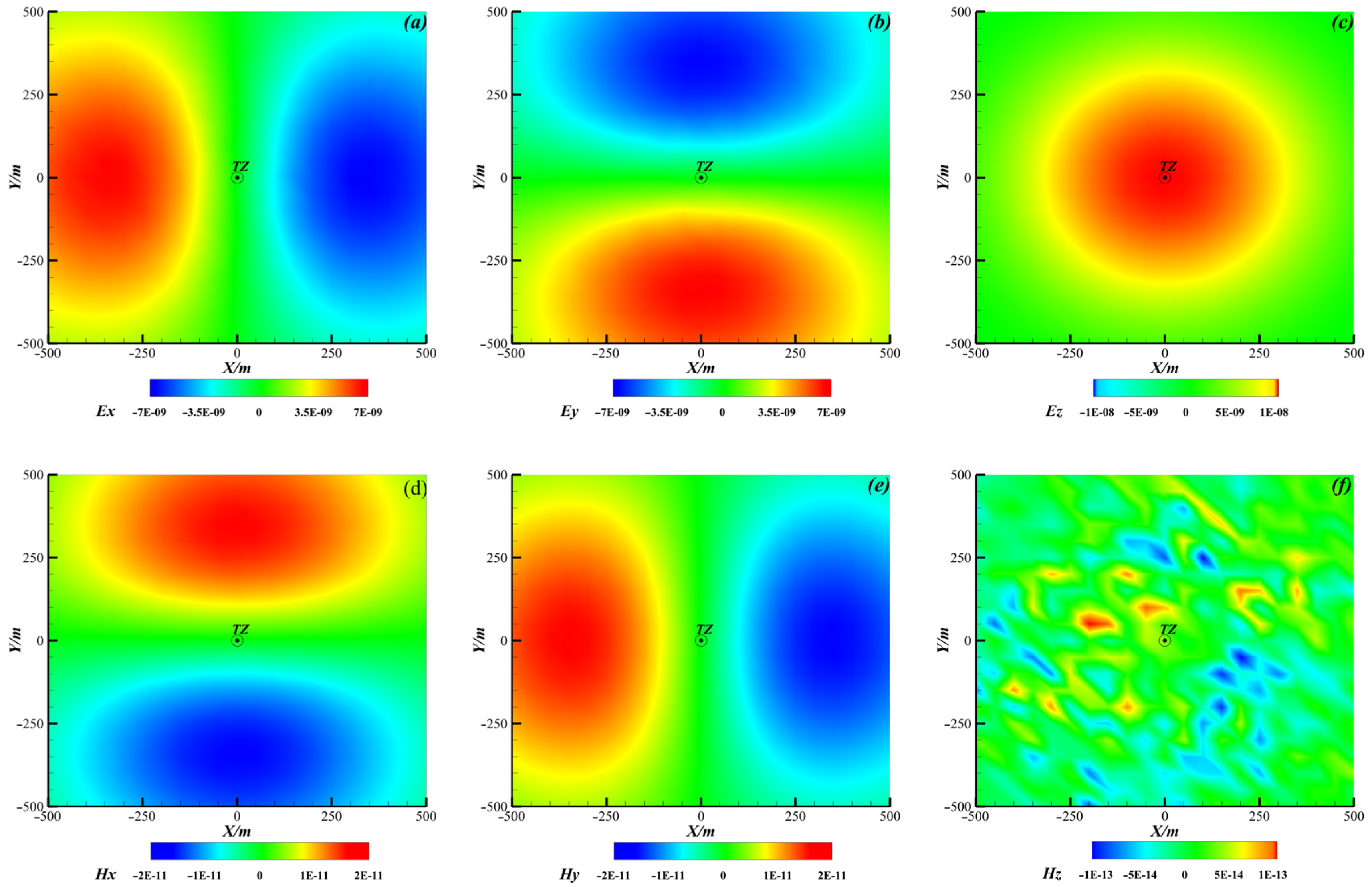
Analyzing the fields excited by a Vertical Electric Dipole (VED) produced by marine VED sources is essential for enhancing the geometric arrangement of transmitters and receiver stations during field operations. A well-structured survey line design should guarantee that receivers are located in areas where the target electromagnetic fields exhibit strong signal intensity and consistent spatial distribution. This study calculated the response values of six electromagnetic fields at a depth of 900 m at two specific time gates: early time (0.01 s) and late time (0.1 s), and presented their planar distribution maps (refer to Figure 2). The simulation domain encompasses an area of 1000 m × 1000 m, with coordinates in the x and y directions extending from −500 m to 500 m.

Figure 2 depicts the planar distribution characteristics of the underground VSTEM fields generated by VED sources at t = 0.01 s. The examination of this figure indicates the ensuing findings: The extreme value region of the Ex field shows a dipole-like distribution that is symmetric on both the left and right sides, with its center positioned directly beneath the transmitter. The distribution of field values is continuous and uniform along the y-axis, nearing zero exclusively on the central axis where x = 0. The extreme value region of the Ey field exhibits symmetry concerning the point directly beneath the transmitter and its perpendicular bisector. This region demonstrates an orthogonal relationship to the Ex field. The distribution of field values is continuous and uniform along the x-axis, with the field value reaching zero along the symmetry axis at y = 0. The extreme value region of the Ez field creates an axially symmetric ring distribution centered directly beneath the transmitter. The field value reaches its peak in the central area and decreases uniformly with a radial gradient outward in all directions. There are no zero-value regions or polarity reversals throughout the entire plane, which indicates optimal distribution stability. The distribution characteristics of the dHx/dt field closely resemble those of the Ey field, exhibiting extreme values along the positive and negative y-axis directions, while the field value remains zero on the symmetry axis at x = 0. The extreme value region of the dHy/dt field is located on both the positive and negative sides of the transmitter along the x-axis, exhibiting a distribution pattern that closely aligns with the Ex field. The dHz/dt field displays low field values throughout the entire plane, which restricts its practical application in real-world exploration.

HxHyHxHyMarine VSTEM methods primarily utilize fixed seabed array observations or towed continuous profile observations. Therefore, the selection of observation time windows and the spatial arrangement of survey points must be carefully designed in conjunction with the temporal diffusion laws of the transient field. Consequently, the five components (Ex, Ey, Ez, dHx/dt, dHy/dt) are all appropriate for practical observation during the designated observation time window: To achieve stable and effective signals for the Ex, Ey, dHx/dt, and dHy/dt fields, which exhibit zero-value symmetry axes, it is essential to design the geometric relationship between the transmitter and survey points carefully. Specifically, the receiver points should be positioned outside the axial regions where the field values of the corresponding components are zero, ensuring optimal signal acquisition throughout the entire time window. The dHz/dt field shows very low values during the entire observation period. Its effective signals are easily obscured by marine environmental noise and instrument background noise, making it practically unobservable throughout the survey.

This study focuses on analyzing the vertical diffusion laws of the VSTEM field originating from marine VED sources within seabed strata that exhibit typical electrical anomalies. The objective is to explain the influence mechanisms of different resistivity anomaly layers on the characteristics of transient field propagation. To accomplish this, two varieties of three-layer geoelectric models were developed, representing real-world situations in marine VSTEM exploration: the H-type conductive anomaly model and the K-type resistive anomaly model.

Table 1. Model parameters.

Model	H1 (m)	H2 (m)	ρ1 (Ω·m)	ρ2 (Ω·m)	ρ3 (Ω·m)
H	1000	100	10	1	10
K	1000	100	10	100	10

presents the model parameters. The vertical profile distribution characteristics of the Ex field, Ey field, Ez field, dHx/dt field, and dHy/dt field, as excited by the VED sources, were simulated at three specific time instances: 0.01 s, 0.1 s, and 0.5 s. The profiles align with the strike of the transmitting source, extending from depths of 0 to 2000 m beneath the seabed and spanning a lateral range of −1000 m to 1000 m. The field values are presented in base-10 logarithmic format following the application of their absolute values. 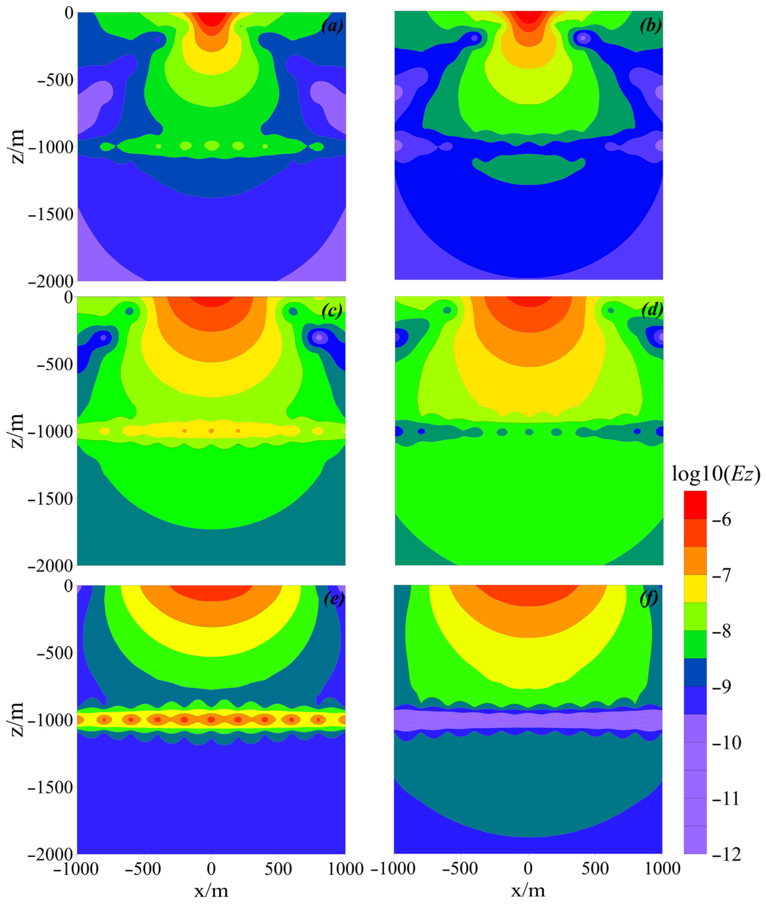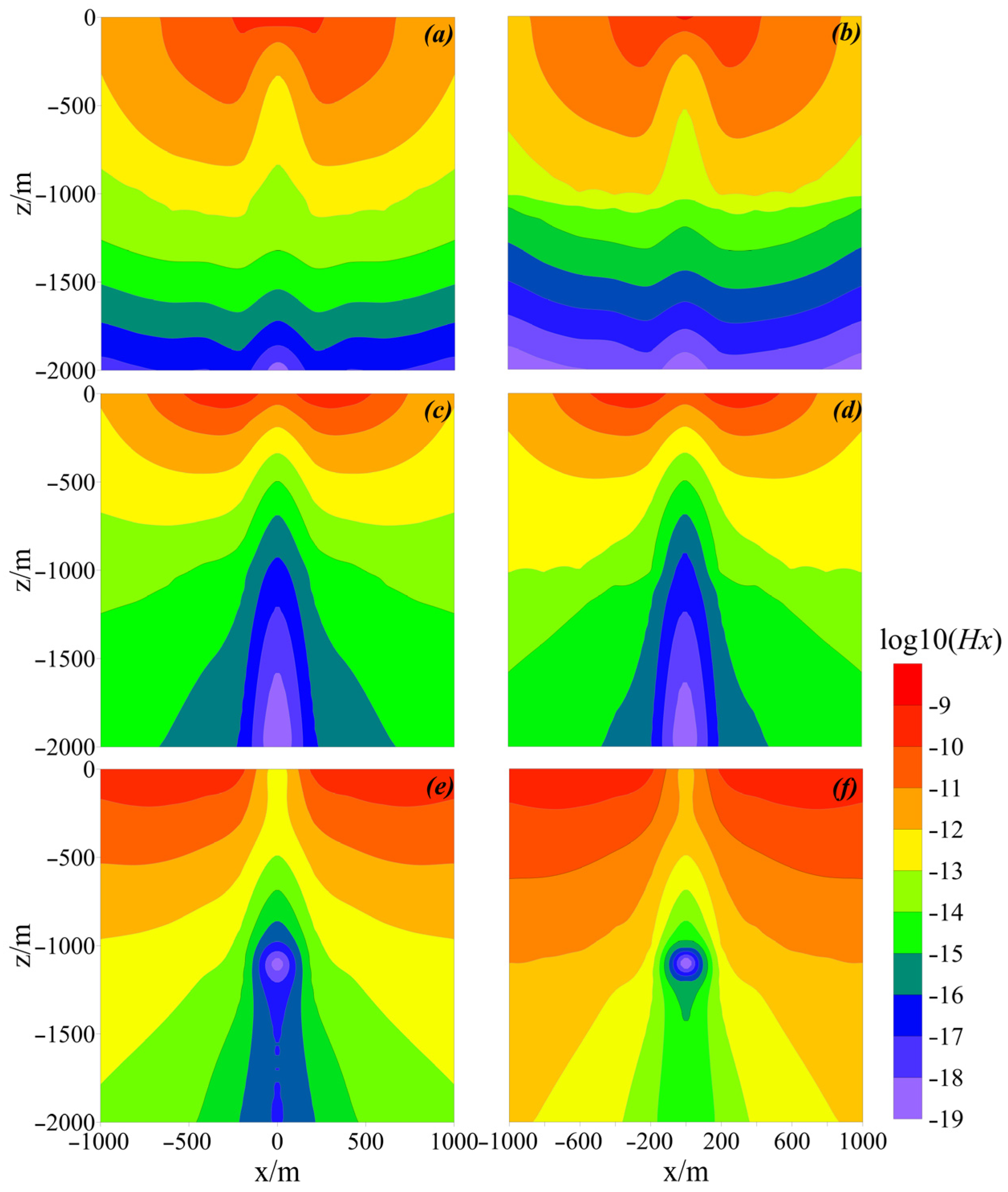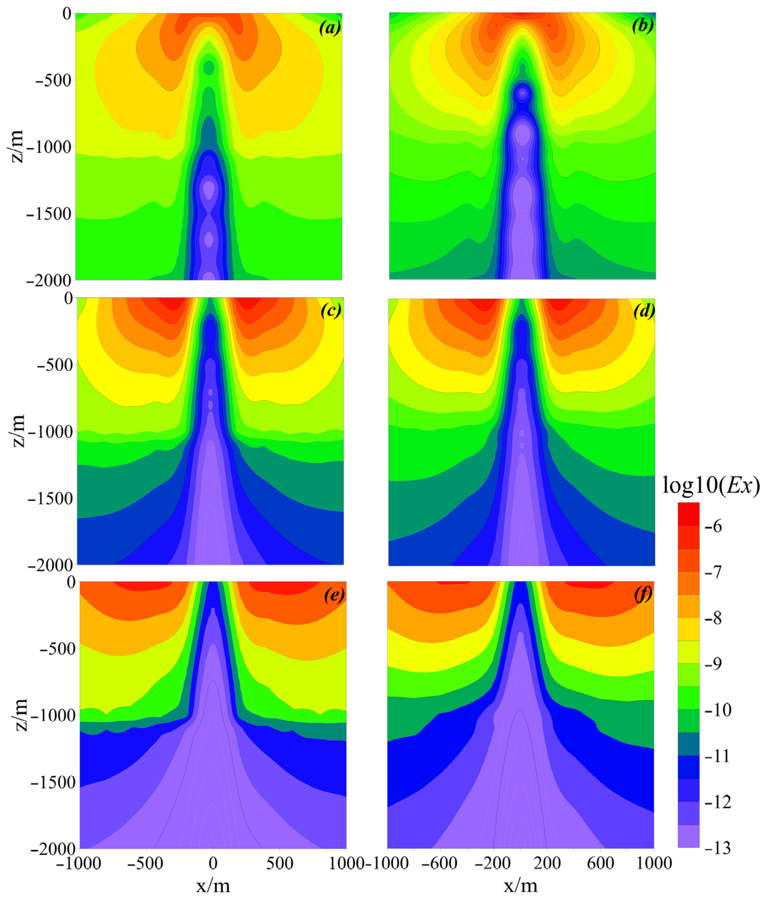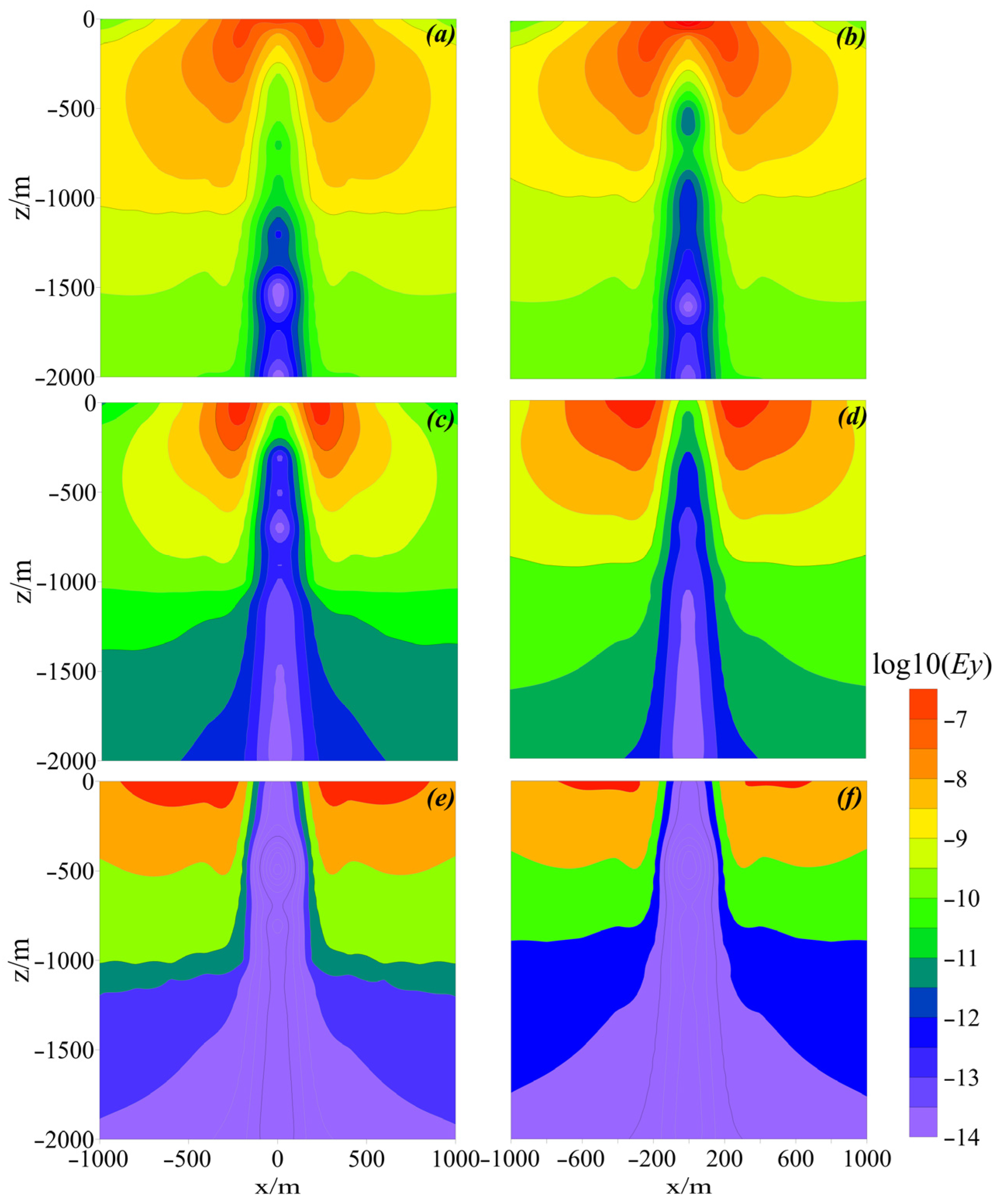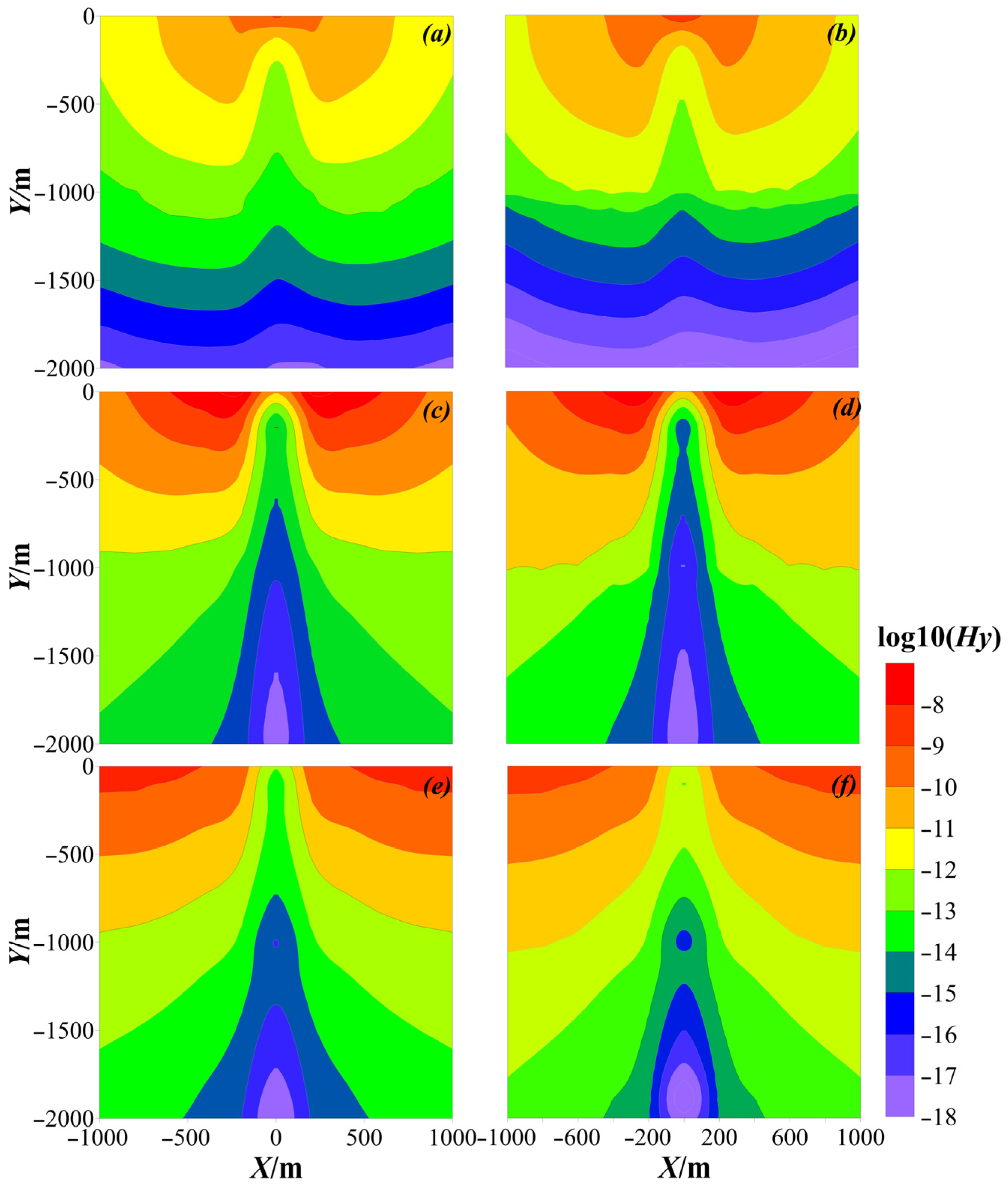Figure 3, Figure 4, Figure 5, Figure 6 and Figure 7 illustrate the vertical diffusion maps for Ex, Ey, Ez, dHx/dt, and dHy/dt, respectively. Each figure presents the simulation results for the H-type model on the left side (a,c,e), and the results for the K-type model on the right side (b,d,f). Additionally, in each figure, the first row (a,b), the second row (c,d), and the third row (e,f) represent the vertical diffusion maps at 0.01 s, 0.1 s, and 0.5 s, respectively.

Figure 3 indicates the vertical diffusion maps of the Ex field at various time instances, displaying a logarithmic distribution range of field values from −6 to −13. The total strength of the electric field is considerably greater than that of the magnetic field. At the initial stage (0.01 s), the region of elevated values in the Ex field has already progressed downward along the central axis to a depth of 2000 m, significantly ahead of the associated magnetic fields. The data show that the vertical diffusion velocity of electric fields is considerably greater than that of magnetic fields, enabling penetration into the anomaly layers even at early stages. At this stage, a minor distinction in field distribution between the resistive and conductive models is noted: the shallow field values in the K-type model are marginally greater than those in the H-type model, indicating the initial shielding effect of the resistive layer on the early electric field, with field energy starting to accumulate above the resistive layer.

At the intermediate stage (0.1 s), separate variations are noted in the Ex field distribution between the two models. The H-type model illustrates that the high-value band of the Ex field exhibits important narrowing and accumulation within the conductive layer at a depth of 1000 m. Field values establish local extrema within this layer, resulting in a notable reduction in diffusion velocity. The occurrence of this phenomenon is attributed to a substantial increase in the induced current density within the conductive layer, which results in significant dissipation of electric field energy. The K-type model shows a notable change in the amplitude of the Ex field as it traverses the resistive layer at a depth of 1000 m. The field values that exceed the resistive layer exhibit a significant increase, whereas those located within and beneath the layer diminish swiftly. Contour lines display a clear vertical displacement at the resistive layer, indicating its significant shielding effect on the electric field. Induced currents face challenges in developing within the resistive layer, which hinders the efficient downward transmission of electric field energy; as a result, a significant portion of energy stays trapped above the resistive layer.

In the final phase (0.5 s), the H-type model demonstrates that the high-value region of the Ex field consistently gathers at the conductive layer depth (1000 m), resulting in the formation of a closed high-value trap within that layer. The gradients of field values above and below the conductive layer are significantly large, resulting in highly stable identification characteristics of the conductive anomaly. The K-type model indicates an overall upward shift in the high-value zone of the Ex field. A specific low-value belt is established at the location of the resistive layer, situated at a depth of 1000 m. Values in the field above the resistive layer have experienced global attenuation, whereas values in deeper fields exhibit only minimal diffusion. The resistive layer maintains a consistent shielding effect on the vertical propagation of the late-stage electric field. The main identification feature for the resistive anomaly is defined by this layered low-value belt.

Figure 4 shows the vertical diffusion maps of the Ey field across various time instances. The Ey field is distributed orthogonally in relation to the Ex field. The response pattern to resistive anomalies aligns with that of the Ex field; however, it demonstrates enhanced lateral focusing and improved identification accuracy for thin resistive layers. During the initial phase (0.01 s), the distinction in shallow field values between the resistive and conductive models is more evident in the Ey field compared to the Ex field, suggesting a greater effectiveness in the early detection of resistive anomalies. During the intermediate stage (0.1 s), the amplitude mutation of the Ey field at the position of the resistive layer is more significant, resulting in enhanced identification characteristics for both the upper and lower interfaces of the resistive layer. At the late stage (0.5 s), the low-value anomaly belt created by the Ey field in the resistive model exhibits more defined boundaries, indicating enhanced accuracy in identifying vertical and lateral boundaries for thin resistive layers when compared to the Ex field.

Figure 5 presents the vertical diffusion maps of the Ez field at various time instances, featuring a logarithmic distribution range from −6 to −12. At the initial phase (0.01 s), the elevated region of the Ez field is localized in the near-surface area (0–500 m), exhibiting an axisymmetric ring-like pattern. A clear horizontal low-value zone is established at a depth of 1000 m, whereas deeper field values decline quickly. This indicates the layered distribution features of the vertical electric field during the initial periods and highlights its significant responsiveness to stratigraphic boundaries. This feature arises from the charge accumulation effect of the vertical electric field at electrical interfaces. At stratigraphic boundaries where resistivity changes abruptly, charges of opposite signs accumulate. These function as a series of electric dipoles oriented perpendicular to the interface, resulting in notable variations in the Ez field at the interface.

During the intermediate stage (0.1 s), the high-value region of the Ez field shifts downward as a complete entity. A continuous horizontal high-value belt is established at a depth of 1000 m, with field values exhibiting distinct segmented characteristics throughout the vertical profile, extending to a depth of 2000 m. The horizontal layered distribution pattern of the contour lines shows a marked enhancement, suggesting that the mid-stage Ez field has effectively penetrated through strata at different depths and has created stable field anomalies at electrical interfaces.

At the late stage (0.5 s), the high-value belt of the Ez field reaches stability at a depth of 1000 m. Field values in both shallow and deep regions exhibit significant decay, leaving only a continuous, closed high-value anomaly present at this particular depth. The horizontal continuity of the contour lines is notably robust, indicating the accurate identification capability of the late-stage Ez field for stratigraphic electrical interfaces. The distribution of its field anomalies along horizontal interfaces illustrates a vertical resolution that significantly exceeds that of horizontal electric and magnetic fields.

Figure 6 depicts the vertical diffusion maps of the dHx/dt field at various time instances, with the logarithmic distribution range of field values extending from −9 to −19. During the initial phase (0.01 s), the area of high values in the dHx/dt field is focused within the shallow strata, specifically between 0 and 500 m below the seabed. The contour lines typically display a nearly horizontal layered arrangement, with a minor downward bulge noted along the central axis of the transmitter source (X = 0 m). The field distributions observed in the H-type model and the K-type model exhibit negligible differences, suggesting that the energy from the early transient field has yet to reach the anomaly layer located at a depth of 1000 m. As a result, the resistive and conductive anomalies do not significantly influence the shallow field distribution; rather, the propagation of the field is mainly determined by the conductivity properties of the overlying background layers.

At the intermediate stage (0.1 s), the transient field energy has reached the anomaly layers, leading to notable differences in field distribution between the two models. In the H-type model, the high-value zone of the dHx/dt field reaches a depth of 1500 m. Distinct field value accumulation takes place at the conductive layer position (1000 m depth), characterized by narrowing contour lines within the layer and a significant reduction in diffusion velocity. Conversely, in the K-type model, the high-value zone of the dHx/dt field shows a distinct amplitude change as it traverses the resistive layer at a depth of 1000 m. The field values present above the resistive layer are significantly higher than those in the H-type model at the same time. In contrast, the values present within and beneath the layer demonstrate a rapid decline. At the late stage (0.5 s), differences in field distribution between the two models become more apparent. The H-type model indicates that the high-value anomaly of the Hx field is consistently located at the conductive layer depth of 1000 m. Field values establish a closed high-value trap within the conductive layer, whereas values beneath the layer diminish quickly. This shows the prolonged accumulation impact of the conductive body on magnetic field energy, resulting in unique identification characteristics for conductive anomalies. In the K-type model, there is an overall upward shift in the high-value zone of the dHx/dt field. A unique low-value belt is established at the position of the resistive layer, located at a depth of 1000 m. The values in the field above the resistive layer have diminished considerably, while the deep field values exhibit only minimal diffusion. This shows that the resistive layer maintains a continuous shielding effect on the vertical propagation of the late-stage magnetic field. The response of field values to resistive anomalies is primarily characterized by low-value anomalies, serving as the core identification marker.

Figure 7 presents the vertical diffusion maps of the dHy/dt field at different time instances, showcasing a logarithmic distribution range of field values from −8 to −18. The overall magnitude of the field surpasses that of the Hx field, and its response patterns to resistive and conductive anomalies exhibit certain similarities to those of the dHx/dt field. During the initial phase (0.01 s), the high-value region of the dHy/dt field is similarly focused in the shallow layers (0–500 m), showing no notable variations in field distribution between the resistive and conductive models, which aligns with the characteristics of the dHx/dt field at the same moment.

During the intermediate stage (0.1 s), the differentiation characteristics between the resistive and conductive models for the dHy/dt field are significantly more pronounced compared to those for the dHx/dt field. The H-type model indicates that the high-value band of the dHy/dt field creates a clear accumulation within the conductive layer at a depth of 1000 m. The contour lines become significantly narrower within this layer, and there is a notable decrease in the vertical diffusion velocity, underscoring the pronounced confinement effect of the conductive layer on the field. The dHy/dt field in the K-type model shows a notable amplitude mutation at the position of the resistive layer. A distinct high-value accumulation develops above the resistive layer, whereas field values within and beneath the layer experience a steep decline. The response characteristics of the resistive interface are more distinct compared to those of the dHx/dt field. This suggests that the dHy/dt field exhibits greater sensitivity to vertical electrical variations within the strata, making it more effective for detecting thin-layer anomalies.

At the late stage (0.5 s), in the H-type model, the dHy/dt field exhibits a well-defined, closed high-value anomaly core located at the conductive layer position (1000 m depth). The gradient of the field value throughout the conductive layer is significantly pronounced, resulting in a clearly defined identification marker for the conductive anomaly. The dHy/dt field in the K-type resistive model creates a notable low-value anomaly belt at the position of the resistive layer, located at a depth of 1000 m. The distinguishing features of field values situated above and below the resistive layer are evident, showcasing a notably enhanced ability to detect resistive anomalies in comparison to the dHx/dt field.

3.2. Analysis of Target Resolution Capability Under Different Transmitter Configurations

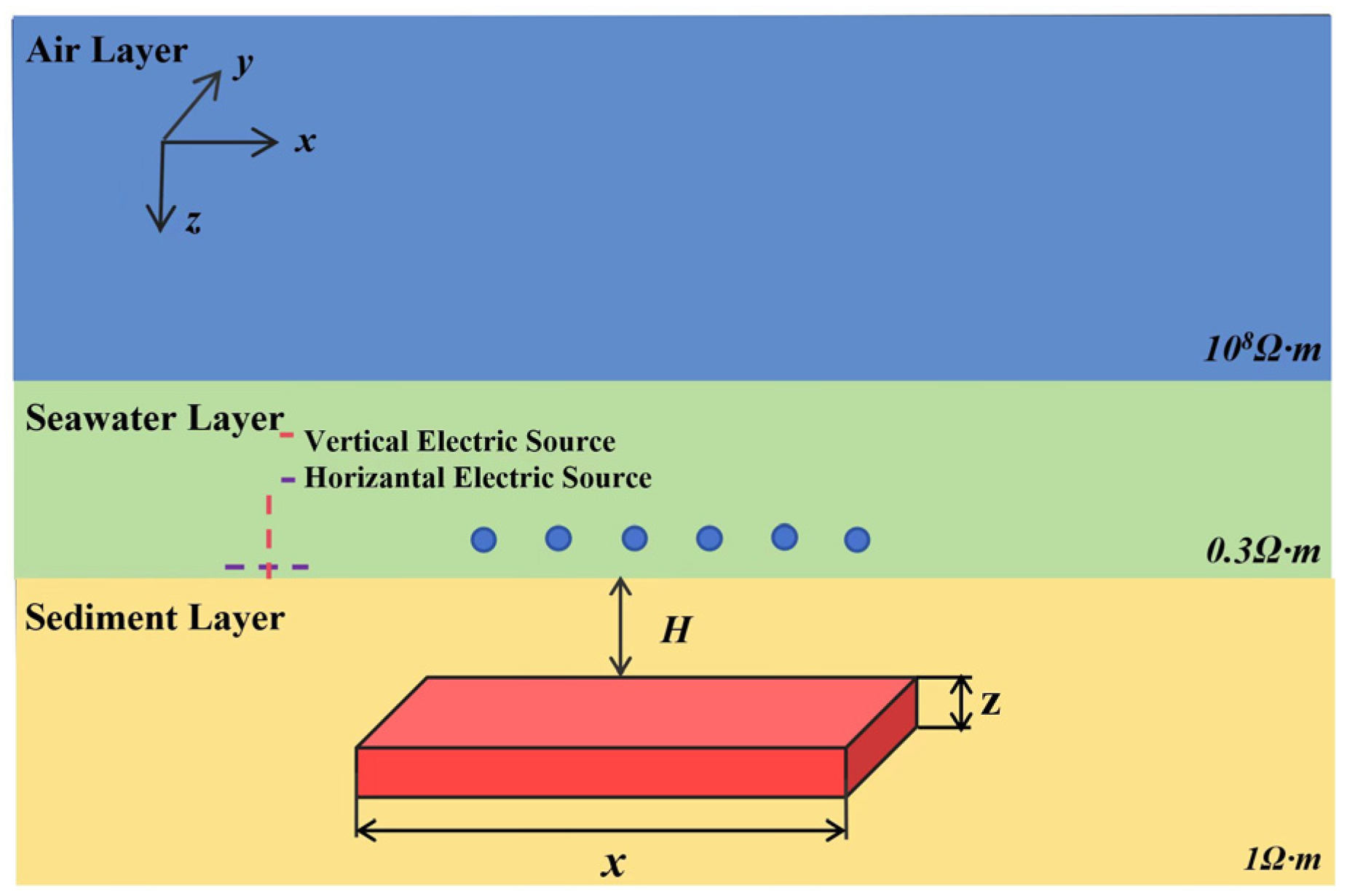
A layered marine model, illustrated in Figure 8, is used to assess the resolution capability of different transmitter configurations concerning variations in the target’s x-direction. The model consists of a 500 m thick seawater layer with a resistivity of 0.3 Ω·m, an air layer that has a resistivity of 10⁸ Ω·m, and a seabed sediment layer below it with a resistivity of 1 Ω·m.

A resistive hydrocarbon reservoir anomaly is located within the sediment layer, characterized by a resistivity of 100 Ω·m. The anomaly has defined dimensions of 4000 m in the y-direction and 200 m in the z-direction, with its extension length in the x-direction varying between two scenarios: 2000 m and 4000 m. The anomaly’s center is positioned at the coordinates (0, 0, −700).

Two configurations for the transmitter are examined: a horizontal long wire and a vertical long wire. The two sources each measure 300 m in length, with their centers located at coordinates (−6000, 0, 40) and (−6000, 0, 190), respectively. Each source is divided into a superposition of 100 uniform electric dipoles. A current of 1 A is applied using a downward step-off waveform.

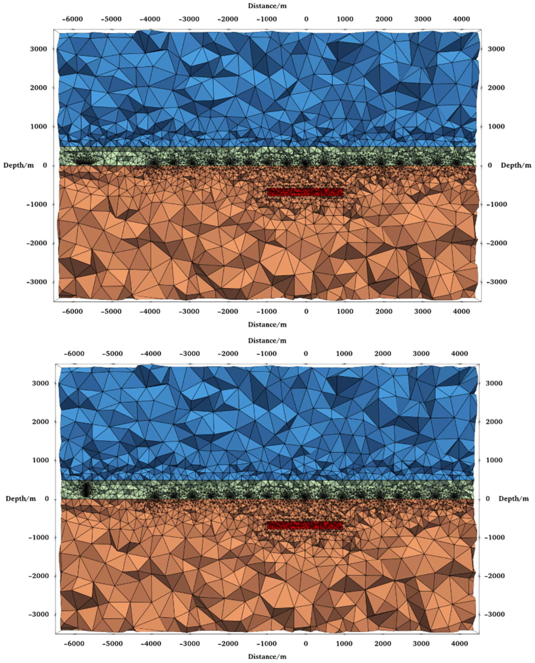
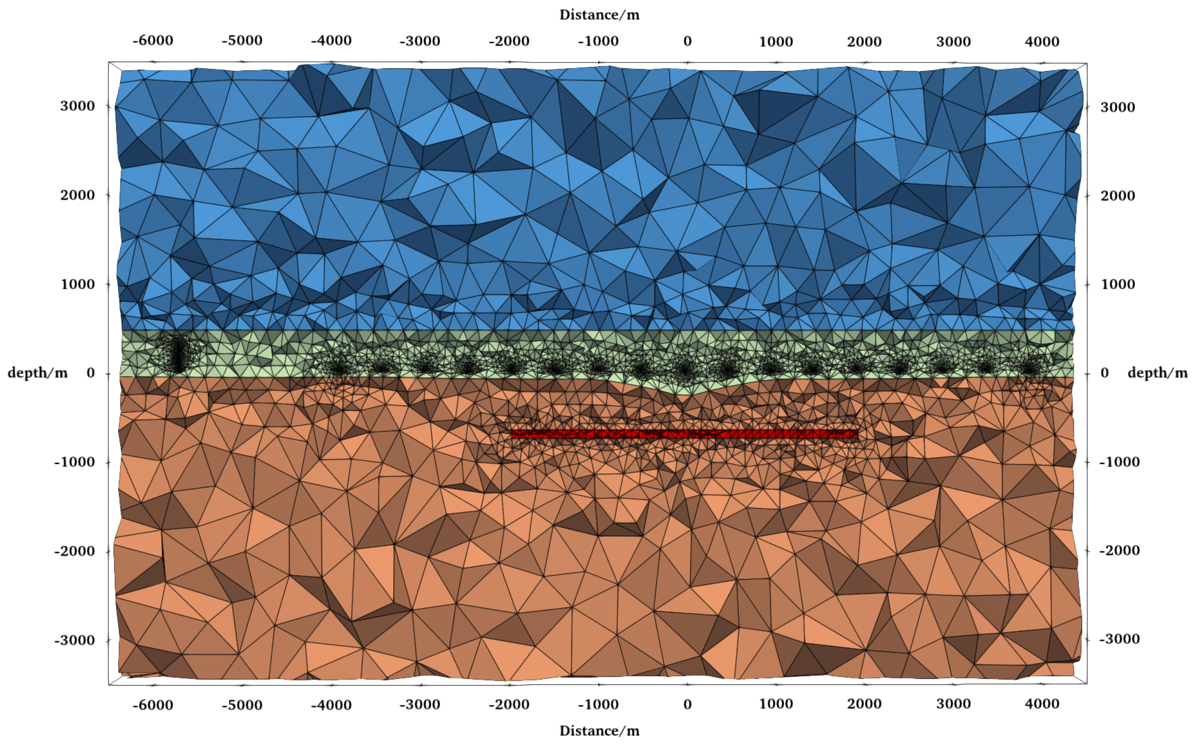
Receivers are positioned at a height of 40 m above the seabed. Local mesh refinement is implemented around the transmitter and receiver locations to guarantee numerical precision. Figure 9 and Figure 10 shows the mesh discretization of the model for the scenario in which the anomaly’s length in the x-direction measures 2000 m.

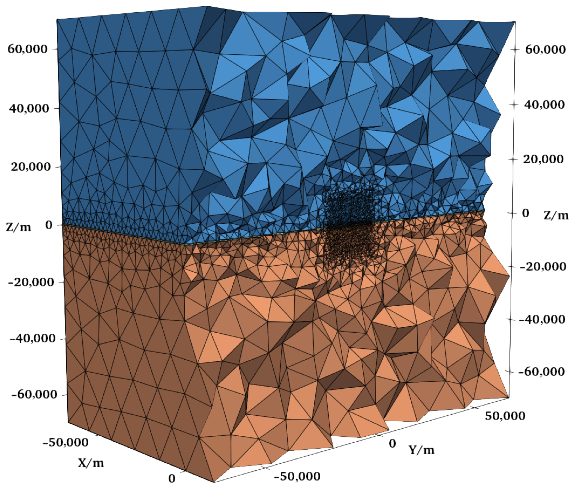
The 3D numerical model was discretized using unstructured tetrahedral meshes, as illustrated in Figure 9. The entire computational domain spans 140,000 m, 140,000 m and 140,000 m in the X, Y and Z directions, respectively. To balance numerical accuracy and computational efficiency, a local mesh refinement strategy was adopted: the core region with a size of 20,000 m × 20,000 m × 20,000 m was discretized with dense meshes, while the mesh size was gradually coarsened towards the outer boundary of the domain. The cross-section at the x = 0 plane is provided to clearly demonstrate the spatial distribution characteristics of the meshes. For the homogeneous full-space model, the computational domain is discretized into 592,794 unstructured tetrahedral elements with a corresponding total of 100,432 nodes.

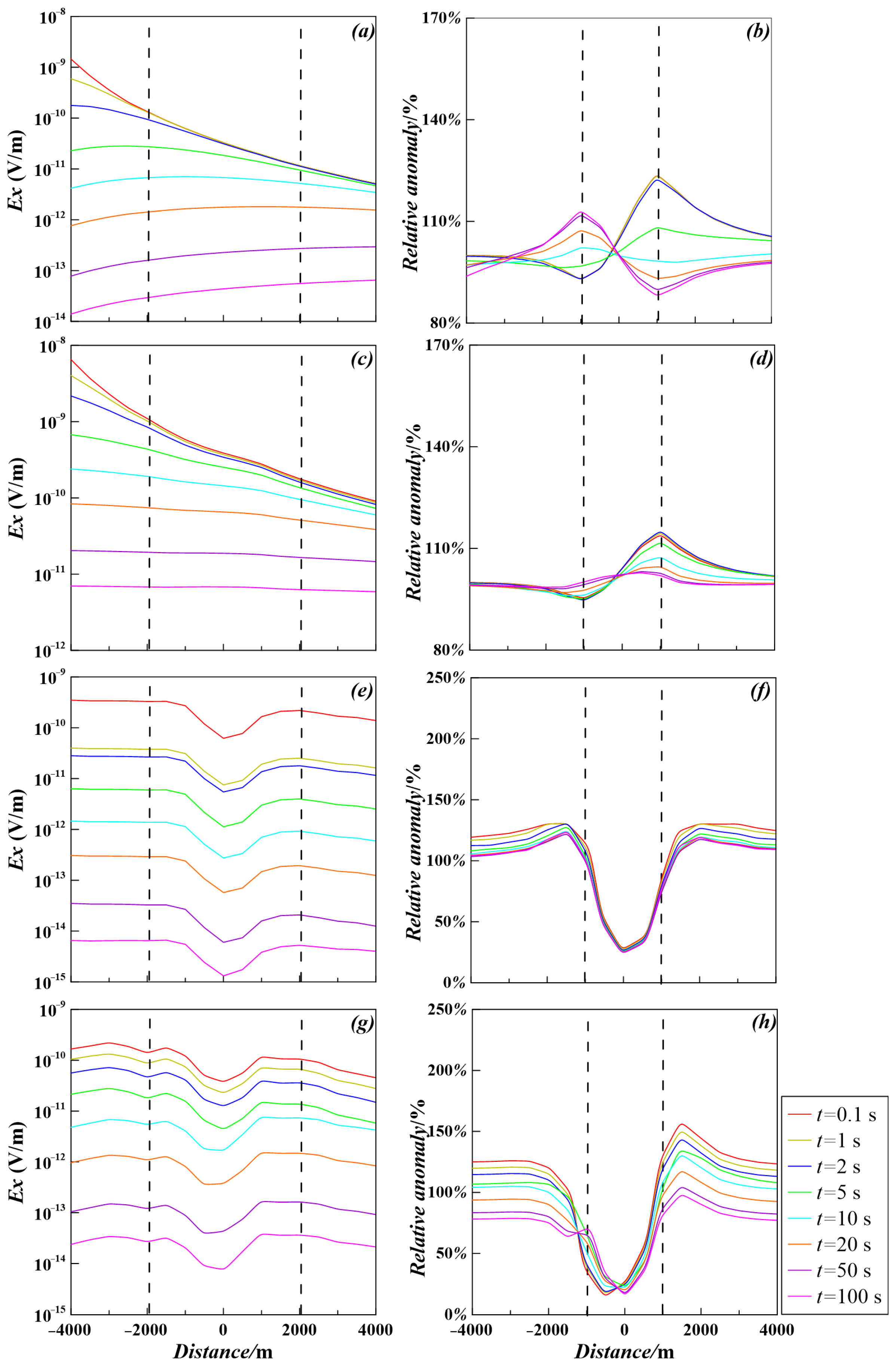
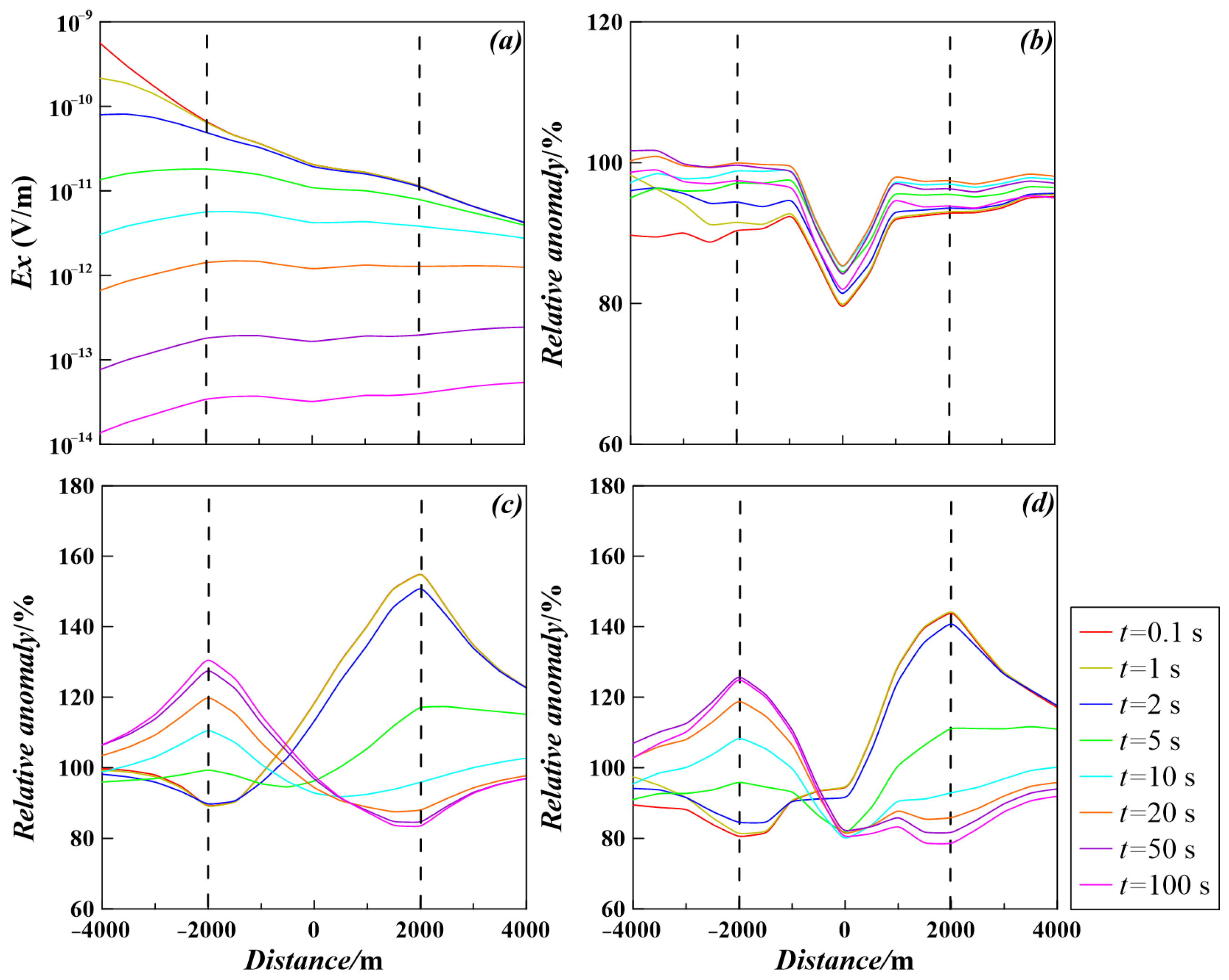
Figure 11 and Figure 12 illustrate the profile curves of the Ex and Ez fields, along with their corresponding relative anomaly responses (defined as the ratio of responses with and without the anomaly), for anomalies extending 2000 m and 4000 m in the x-direction, respectively, excited by vertical and horizontal sources. Figure 11a shows the amplitude distribution of the Ex field generated by the VED. The Ex field profiles show clear morphological changes at the anomaly boundaries, creating distinct inflection points that can be utilized to determine the lateral extent of the anomaly. The relative anomaly curve presented in Figure 11b closely corresponds with the anomaly boundaries, exhibiting a “trough-peak” pattern during the early time intervals, which transitions into a “peak-trough” pattern as time progresses. The positions of the anomaly peaks and troughs consistently remain fixed at the ±2000 m boundary coordinates, showing no spatial shift over time. This component showcases remarkable precision in positioning the lateral boundaries and scale of the anomaly, achieving a maximum relative anomaly amplitude that surpasses 123%, while the minimum falls to 88%. Figure 11e illustrates the amplitude distribution of the Ez field generated by the VED. Inflection points are present at the boundaries in the Ez field profiles; however, their positions are notably altered. The relative anomaly curve (Figure 11f) reveals a stable morphology throughout both early and late times, showing notable low-value zones around ±1500 m. Although the anomaly contrast of the Ez field is significantly high with a maximum amplitude surpassing 128%, a minimum falling to 25%, and a total variation range of 103%, the locations of its extrema are shifted inward by about 500 m compared to the actual boundaries (±2000 m), resulting in imprecise boundary localization.

Figure 11c shows the amplitude distribution of the Ex field generated by the horizontal source. The distribution trend of the horizontal source Ex field resembles that of the VED. Throughout both early and late periods, the relative anomaly curve exhibits distinct “trough-peak” features at the boundaries, achieving a maximum amplitude that surpasses 114% and a minimum of 95%. Figure 11g demonstrates the amplitude distribution of the Ez field generated by the horizontal source. The horizontal source Ez field shows a distinct low-value area within the anomaly range; however, the center of this area does not align with the geometric center of the anomaly. The relative anomaly curve indicates low values between −2000 m and 1500 m, featuring a maximum amplitude that surpasses 155% and a minimum that falls to 16%. Although there is a very strong signal contrast, the peak positions do not align with the actual boundaries, which complicates the accurate delineation of the anomaly edges.

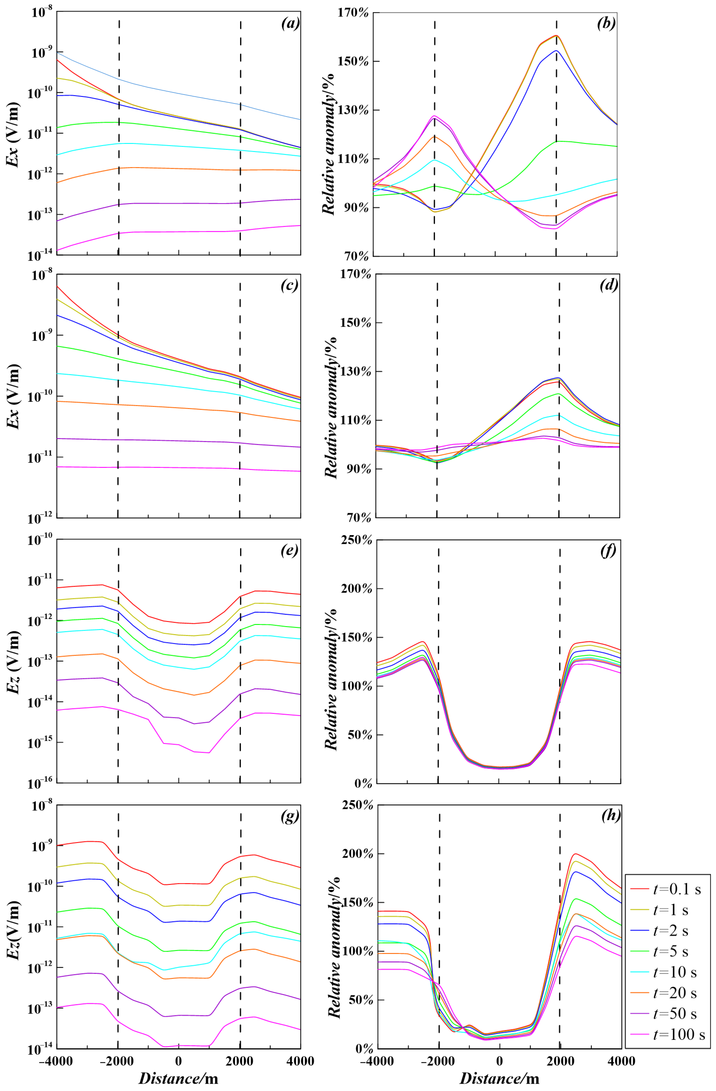
Figure 12 demonstrates the electric field responses for both horizontal and VED sources, when the scale of the anomaly is increased, with the anomaly extending 4000 m in the xx-direction. Figure 12a illustrates the amplitude distribution of the Ex field produced by the VSTEM. The Ex field profiles delineate more distinct and precise inflection points at ±4000 m, accurately aligning with the actual boundaries of the anomaly. The relative anomaly curve (Figure 12b) maintains the evolutionary pattern of “early-time trough-peak” and “late-time peak-trough,” with the peak and trough positions consistently fixed at ±4000 m. The maximum relative anomaly amplitude rises to 162%, whereas the minimum decreases to 87%, demonstrating that the VSTEM Ex field preserves outstanding boundary identification precision even in the presence of significant anomaly conditions.

Figure 12e,f display the amplitude distribution and relative anomaly curves of the Ez field excited by the VSTEM. The Ez field maintains notable contrast features, with a maximum amplitude surpassing 132% and a minimum decreasing to 12%. Nonetheless, it establishes a continuous low-value area around ±3500 m, resulting in a discrepancy of roughly 500 m between its edges and the actual boundaries at ±4000 m. This indicates that the Ez field encounters difficulties in attaining accurate boundary localization.

The integration of the response characteristics from both models, utilizing anomaly lengths of 2000 m and 4000 m in the x-direction, reveals that the Ex field generated by the VSTEM exhibits enhanced precision in boundary identification accuracy. In both models, the inflection points of the field values and the peak-trough positions of the relative anomaly curves align precisely with the true boundaries of the anomaly, demonstrating no spatial displacement. The identification accuracy remains stable even when the anomaly scale is doubled, with only the polarity of the peaks and troughs reversing over time. The horizontal source Ex field demonstrates restricted identification capability primarily during early to intermediate times, exhibiting poor performance at later times. In the meantime, the Ez field, irrespective of the source type, can indicate the presence of an anomaly; however, it shows considerable spatial shifts in all cases, making it inadequate for accurate localization.

In terms of anomaly detection capability, the 2000 m model shows an anomaly amplitude difference for the VSTEM Ex field of 35% (with a maximum of 123% and a minimum of 88%). This is greater than the 19% noted for the horizontal source, which has a maximum of 114% and a minimum of 95%. In the 4000 m model, this difference increases to 75% (maximum 162%, minimum 87%) for the VSTEM, significantly surpassing the 30% observed for the horizontal source (maximum > 124%, minimum 94%). This suggests that the VSTEM Ex field has a superior resolution capability for detecting anomalies when compared to the horizontal source Ex field. In contrast, for the 2000 m model, the amplitude difference for the horizontal source Ez attains 139% (155% compared to 16%), exceeding the 103% observed in the VSTEM Ez. In the 4000 m model, the variation for the horizontal source Ez increases dramatically to 190% (198% compared to 8%), significantly surpassing the VSTEM Ez (120%) and all Ex fields. Consequently, the Ez field is better suited for swift qualitative detection of targets.

3.3. Electromagnetic Response Characteristics of VSTEM Under Undulating Topography

In the setting of marine hydrocarbon exploration, the seabed interface rarely presents as a perfect horizontal layered structure; rather, it is characterized by a variety of complex undulating topographies, including seamount uplifts, trench depressions, and slope zones, which are commonly encountered. The variations in topography lead to distortions in the electromagnetic field, which can obscure or alter the genuine anomaly responses of deep reservoirs, creating considerable challenges for data interpretation. Building upon the previous study of horizontal layered media, this section further focuses on the VSTEM response characteristics under complex seabed topography. This study examines the effects of topographic distortion and its influence on anomaly identification, while also validating the detection adaptability of VED sources in these complex environments.

3.3.1. Seamount Topography

To examine the electric field response characteristics of a VSTEM in relation to undulating seabed topography, a seamount model, as depicted in Figure 13, is utilized. The model is composed of a central seawater layer measuring 500 m in thickness, exhibiting a resistivity of 0.3 Ω·m. Above this layer is an air layer characterized by a resistivity of 10⁸ Ω·m, while below lies a seabed sediment layer with a resistivity of 1 Ω·m. Figure 13 (top) illustrates a seamount measuring 200 m in height, whereas Figure 13 (bottom) presents a seamount with a height of 400 m. The centers of both seamounts are located at x = 0 m, with dimensions measuring 2000 m in both the x and y axes.

A resistive hydrocarbon reservoir anomaly is located within the sediment layer, characterized by a resistivity of 100 Ω·m. The dimensions of the anomaly are established at 4000 m × 4000 m × 100 m, with the center positioned at coordinates (0, 0, −700). The electric-source VSTEM survey configuration is established as an axial array. A long-wire transmitter measuring 300 m in length is situated between 40 m and 340 m above the seabed, with its center located at the coordinates (−5850, 0, 190). The source is divided into a combination of 100 uniform electric dipoles. A current of 1 A is applied in the positive x-direction utilizing a downward step-off waveform. Receivers are positioned along the seabed topography, consistently maintaining a height of 40 m above the seabed surface, with a spacing of 500 m between each receiver. Local mesh refinement is implemented around the transmitter and receiver locations to guarantee numerical precision. The 200 m-high seamount model is discretized with 1,169,762 unstructured tetrahedral elements and 196,228 nodes, while the 400 m-high seamount model adopts a graded mesh scheme with 955,945 elements and 160,715 nodes.

Figure 14a,b indicate the Ex field response curves observed in a resistive hydrocarbon reservoir. The results indicate that the topography of the seafloor seamount has a significant impact on the morphology of the Ex field value curves, resulting in considerable distortion, with fluctuation trends closely corresponding to the undulations of the topography. In regions characterized by important topographical variations, the response amplitude induced by the terrain is substantial, partially masking the weaker response from the deep hydrocarbon reservoir. The direct identification of the target body is facilitated by the absolute field value curves.

Figure 14c,d illustrate the relative percentage anomaly curves for the “model with hydrocarbon reservoir” compared to the “flat seabed + hydrocarbon reservoir” model, specifically under seamount topographies of 200 m and 400 m, respectively. The curves demonstrate a clear “seamount” morphology, with the primary peak precisely aligning with the position of the seamount summit (x = 0). In the 200 m topography (Figure 14c), secondary troughs on either side of the peak are clearly aligned with the seamount boundaries. However, in the 400 m topography (Figure 14d), increased topographic distortion obscures the response characteristics at the seamount boundaries, making them less distinct due to the influence of the main peak anomaly. This suggests that pure topographic influences produce significant false anomalies on relative anomaly curves, exhibiting morphologies that are closely linked to topographic geometric characteristics.

Figure 14e,f illustrate the relative percentage anomaly curves used to evaluate the impact of topography on target identification. These curves compare the “model with topography and hydrocarbon reservoir” against the “model with topography but without hydrocarbon reservoir,” effectively showing the residual anomalies after accounting for the pure topographic effect. Under the 200 m seamount topography (Figure 14e), the curve exhibits clear bipolar characteristics (one peak and one trough) flanking the transmitter source, with the extremum positions closely matching the actual boundaries of the anomaly body (±2000 m). The maximum relative anomaly value attains 163%, surpassing the levels observed under flat seabed conditions. However, the overall curve morphology remains intact, suggesting that the topography does not affect the assessment of the target body’s boundaries. Below the 400 m seamount topography (Figure 14f), the topographic height increases twofold, and the maximum value of the curve reaches 172%. However, the extremum positions on either side of the transmitter source continue to precisely align with the boundaries of the anomaly body, while the morphology of the curve remains consistent. The results indicate that while complex topography affects the absolute amplitude of the electromagnetic field, the vertical Ex field can still effectively delineate the lateral boundaries of resistive targets after applying the “same-topography background subtraction method.” The core characteristics of the anomalous response are slightly affected but not severely distorted by topographic factors., demonstrating that the VSTEM method exhibits strong adaptability and robustness in shallow marine environments with intricate topography.

Figure 14g,h present a comparison of the relative anomalies between the “model with topography and target body” and the “uniform half-space (no topography, no target).” This analysis aims to examine the superposition effect of topographic false anomalies and target true anomalies. Prominent peaks influenced by topography are observed at x = 0 in both scenarios. Below the 200 m seamount topography (Figure 14g), the amplitude of the false anomaly induced by the topography is less than that of the true anomaly generated by the target body; therefore, the characteristics of the target response prevail, and the interference from the topography is minimal. Below the 400 m seamount topography (Figure 14h), the amplitude of the topographic false anomaly markedly surpasses the target response, emerging as the dominant characteristic of the curve. Upon careful observation, it is clear that, against the backdrop of the significant topographic false anomaly, the peak characteristics corresponding to the target body boundaries on both sides of the transmitter source are distinctly identifiable and not entirely submerged. By synthesizing Figure 14e–h, it can be concluded that even in the presence of significant topographic variations (400 m), where topographic false anomalies are prevalent, the characteristics of the target body boundary (peak positions) produced by the VSTEM Ex field remain consistently observable. The topographic effect primarily appears as an increase in amplitude or background distortion, without altering the identified positions of target boundary positions or losing their key characteristic shapes.

3.3.2. Valley Topography

Figure 15 presents the 3-D geoelectric model of a submarine valley. The middle seawater layer is established at a depth of 400 m, exhibiting a resistivity of 0.3 Ω·m, whereas the resistivity of the air layer is defined as 10⁸ Ω·m. The seabed sedimentary layer is characterized by a resistivity of 1 Ω·m. The depth of the valley is established at 200 m, with the center point positioned at x = 0 m; the dimensions in both the x and y directions are defined as 2000 m. A resistive hydrocarbon reservoir anomaly body is located within the seabed sedimentary layer directly beneath the valley, exhibiting a resistivity of 100 Ω·m. The anomaly body has dimensions of 4000 m × 4000 m × 200 m, with its upper boundary located at a burial depth of 400 m beneath the valley floor.

Figure 16a shows the response curves of the Ex field value for the model featuring a resistive hydrocarbon reservoir situated beneath valley topography. The Ex field value distribution, influenced by the concave valley terrain, shows a strong correlation with the topographic morphology. At the valley center (x = 0 m), the notable increase in the thickness of the conductive seawater layer leads to enhanced attenuation of the VSTEM field, which results in a global low-value depression in the field values. As the profile extends laterally to the valley boundaries at approximately 2000 m, the field values progressively recover and rise in alignment with the ascending topography. In these circumstances, the inherent anomalous response of the resistive hydrocarbon reservoir is entirely obscured by the significant topographic distortion, rendering it unfeasible to directly discern the target body from the raw field value curves.

Figure 16b illustrates the relative percentage anomaly curve for the “valley topography + hydrocarbon reservoir” model in comparison to the “flat seabed + hydrocarbon reservoir” model. This curve displays a depression that aligns with the geometric shape of the valley: a notable low-value trough occurs at x = 0 m, directly corresponding to the position of the valley floor, while the inflection points at ±2000 m accurately correspond to the valley boundaries.

Figure 16c provides a comparison of the relative percentage anomaly curves for the “valley topography + hydrocarbon reservoir” model and the “valley topography + no hydrocarbon reservoir” model, specifically focusing on the residual anomalies obtained after eliminating the pure topographic background. The curve exhibits two distinct and independent extrema at ±2000 m, locations that closely correspond with the lateral boundaries of the resistive hydrocarbon reservoir, thereby validating the efficacy of this method in accurately identifying the boundaries of the anomaly body. The maximum relative anomaly value is 158%, indicating a minor amplitude increase when compared to the flat seabed model. The fundamental morphology and the distribution patterns of peaks and troughs are largely in alignment with the flat model. The 200 m deep valley topography does not affect the resolution mechanism of the Ex field for the anomaly body; VSTEM capabilities remain effective even in complex concave terrain.

Figure 16d shows the relative anomaly curve for the “valley topography + hydrocarbon reservoir” model in comparison to the “uniform half-space” model, demonstrating the combined effect of topographic distortion and hydrocarbon reservoir anomalies. While the curve maintains the low value trough characteristics influenced by topography at x = 0 m, in this case, the amplitude of the false anomaly produced by the valley topography is less than that of the true anomaly created by the hydrocarbon reservoir boundaries. The peaks associated with the boundaries of the hydrocarbon reservoir at ±2000 m are distinctly identifiable and remain unaffected by the low-value topographic zone. While topographic distortion is present, it does not interfere with or alter the essential anomalous responses of the hydrocarbon reservoir. Additionally, it does not impact the qualitative assessment of anomaly characteristics or the quantitative determination of boundaries. In conclusion, the 200 m deep concave valley topography mainly leads to distortion in background field values and slight variations in anomaly amplitude for the VSTEM Ex field, yet it does not change the fundamental physical properties of the Ex field in delineating resistive hydrocarbon reservoir boundaries. This result clearly demonstrates that the VSTEM method has stable exploration capabilities and notable advantages in mitigating topographic interference in regions with undulating seabed topography.

3.4. Electromagnetic Response Characteristics of VSTEM Under Complex Geological Conditions

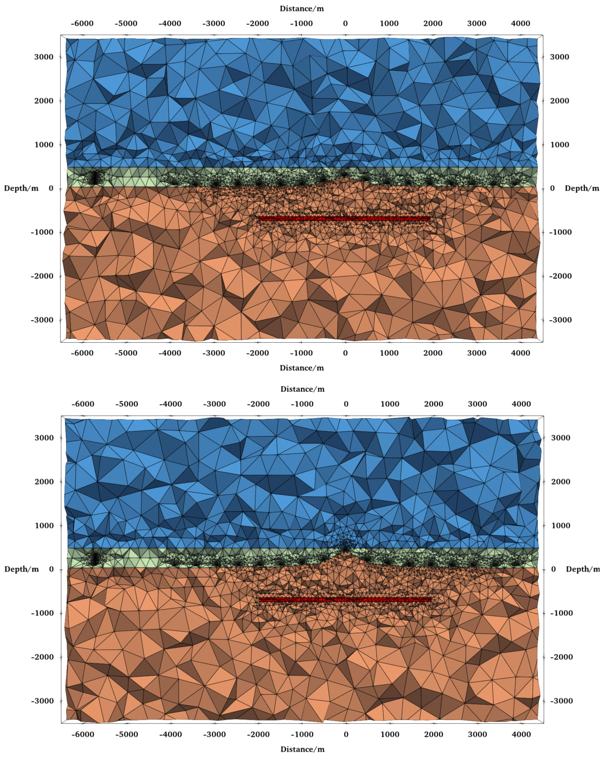
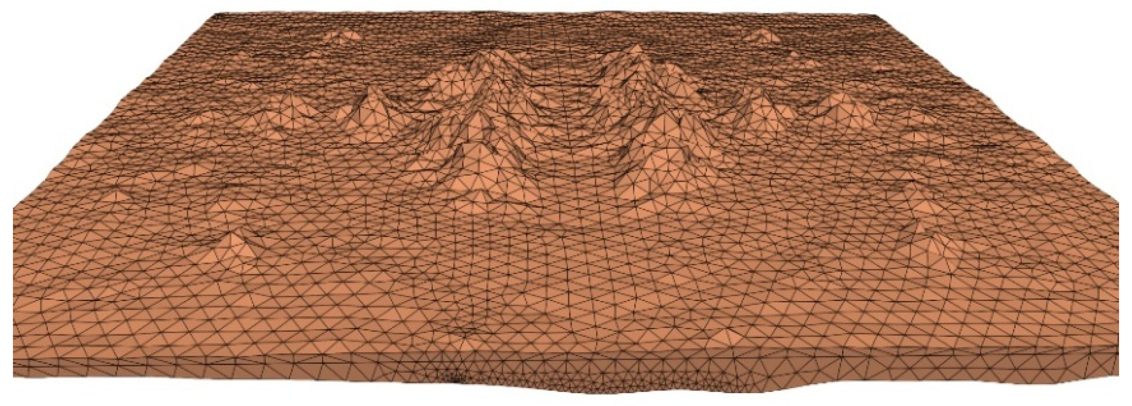
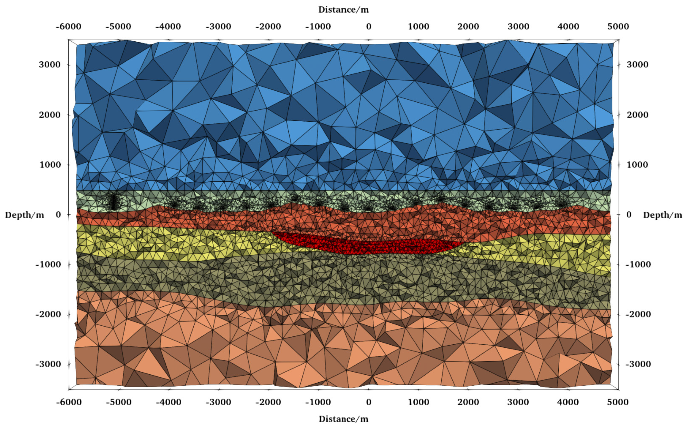
In order to investigate the electric field response characteristics of VSTEM method in relation to complex seabed topography and intricate geological structures, we developed a 3D complex hydrocarbon reservoir model (illustrated in Figure 17 and Figure 18) to replicate actual seabed geological conditions. The model establishes the intermediate seawater layer at a depth of 500 m, characterized by a resistivity of 0.3 Ω·m. In contrast, the overlying air layer exhibits a resistivity of 10⁸ Ω·m. Under the seawater, there are four distinct stratigraphic layers. The initial sedimentary layer exhibits a varied seabed topography with a maximum relief of 250 m and a resistivity measurement of 0.8 Ω·m. The subsequent layers are characterized by resistivities of 1 Ω·m for the second layer, 2 Ω·m for the third layer, and a range of 1/5/10 Ω·m for the fourth layer. For the complex seabed topography and multi-layer stratigraphic model, the computational domain is discretized into 1,398,837 unstructured tetrahedral elements with a corresponding total of 234,852 nodes.

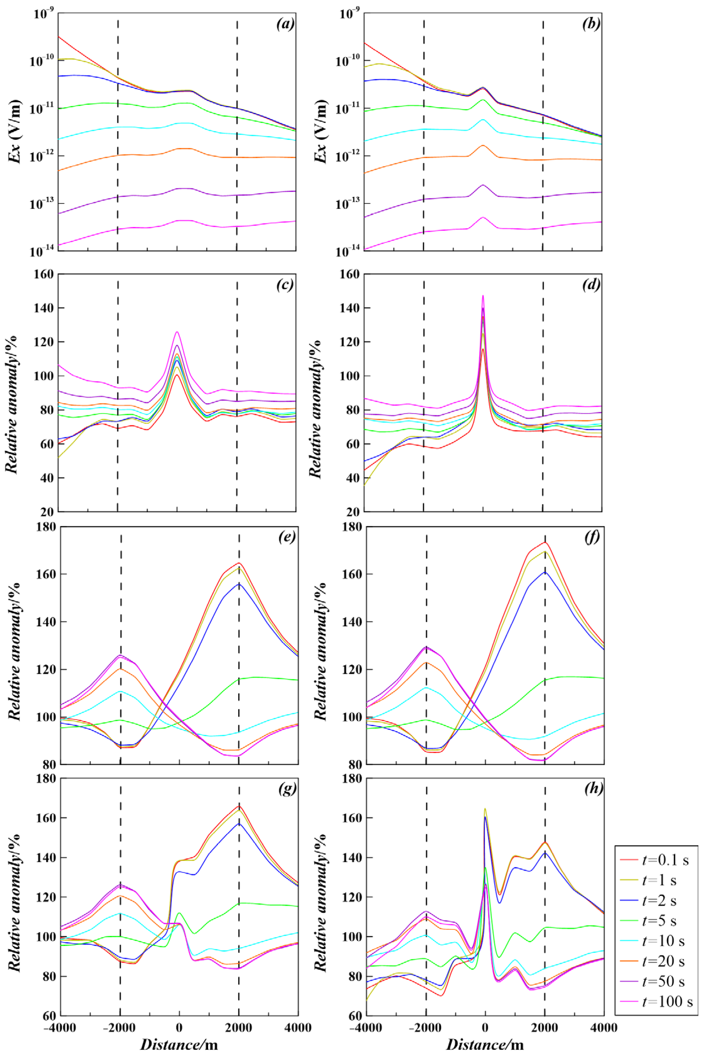
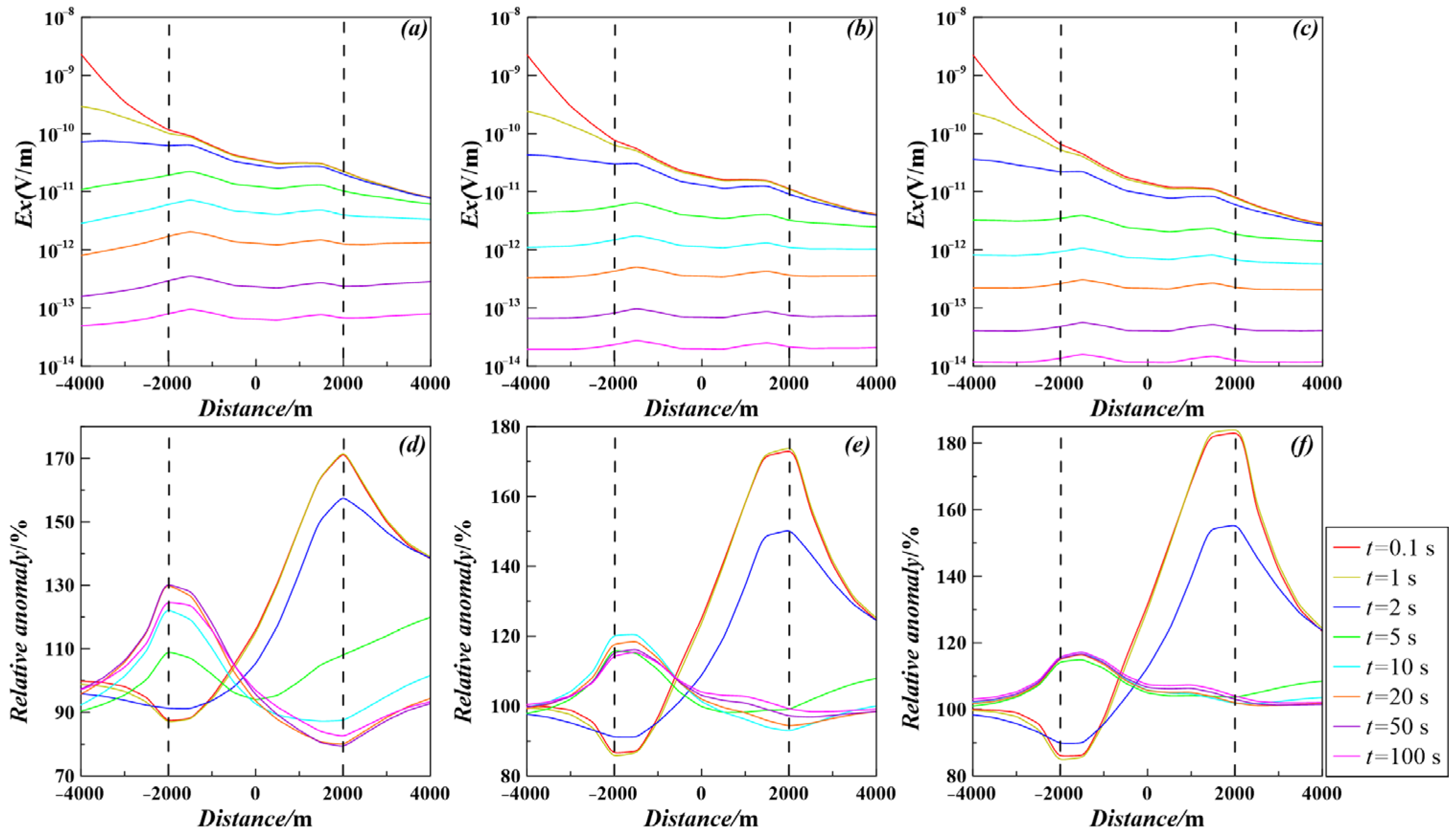
Figure 19 presents the response characteristics of the VSTEM Ex field, highlighting its ability to detect irregular resistive hydrocarbon reservoirs amidst a backdrop of complex undulating seabed topography (250 m relief) and a four-layer geological structure. An analysis of Figure 19a–c indicates that the Ex field values demonstrate a consistent decay trend as the offset increases. Significant local undulations are observed near ±2000 m, a characteristic that closely aligns with the lateral extent of the irregular resistive hydrocarbon reservoir. The local morphology of the field value curves exhibits a significant correlation with the overlying 250 m high seabed topography. Field values indicate local uplifts at topographic highs and display low values in depressions, effectively illustrating the distorting effect of topography on VSTEM field propagation. It is important to note that while the field amplitude exhibits decay over time at various intervals, the overall shape of the curve and its unusual characteristics maintain a high level of consistency.

Figure 19d–f display the curves representing the relative anomaly ratios. The findings indicate that stable and distinct anomaly peaks develop at ±2000 m, with locations accurately aligning with the lateral boundaries of the irregular resistive hydrocarbon reservoir. Despite the significant interference posed by complex topography featuring a 250 m relief and multi-layer geological structures, the Ex field ratio generated by the VSTEM efficiently determines anomaly boundaries, without any instances of anomaly confusion, false anomalies, or boundary shifts. This validates the dependability of this approach in highly intricate settings.

In a comparative analysis of varying working conditions (from left to right), it is observed that as the resistivity of the fourth-layer basement escalates from 1 Ω·m to 10 Ω·m, there is a significant increase in the anomaly peaks at the same time instance. The maximum relative anomaly amplitude rises from 170% to 183%. Additionally, the time window during which the anomaly signal is recognizable is markedly extended. A conductive basement has a significant absorption and attenuation effect on the VSTEM field, leading to a diminished return of field energy from depth, which in turn reduces the anomalous response of the hydrocarbon reservoir. In contrast, a resistive basement exhibits a diminished attenuation effect on the field, thereby promoting the retention and propagation of deep reflected field energy. This greatly enhances the difference in electrical characteristics between the hydrocarbon reservoir and the adjacent rock, facilitating the extraction and detection of subtle anomalies.

In the end, despite the challenging conditions and intricate seabed topography along with multi-layer geological formations, the VSTEM Ex field consistently exhibits reliable performance in delineating the boundaries of resistive anomaly bodies: the peaks of these anomalies align accurately with the lateral boundaries of the hydrocarbon reservoir, showing no spatial displacement or morphological alteration. Furthermore, the resistivity of the deep basement plays a crucial role in influencing the intensity of the anomalous response. An increase in basement resistivity correlates with a higher amplitude of the hydrocarbon reservoir’s anomalous response, an expanded effective detection time window, and enhanced conditions for the precise identification of deep targets.

4. Conclusions

This study applied the advantages of unstructured tetrahedral meshes in TDFEM to characterize complex geometric boundaries, constructing shallow marine geological models. The aim was to achieve 3D forward modeling and analyze the response characteristics of the VSTEM method in intricate environments. The primary conclusions are stated as follows:

This study compares the resolution capabilities of vertical and horizontal sources for target bodies and quantitatively analyzes the detection performance and applicable scenarios of different observation components. The results indicate that the VSTEM Ex field demonstrates significantly superior resolution regarding the spatial morphological variations of the anomaly body in the x and z directions compared to the horizontal source. The positions of the anomaly peaks and troughs completely coincide with the true boundaries of the target body throughout the entire observation time window, showing no spatial shift. Consequently, it serves as an ideal observation component for the detailed characterization of high-resistivity reservoir geometries. Although the Ez field exhibits higher anomaly contrast, it suffers from obvious boundary location offsets, making it more suitable for rapid qualitative detection of target bodies. These findings fully confirm the significant advantages of vertical sources in the fine characterization of deep resistive targets.

The research reveals that even in extreme scenarios involving strongly undulating topography (such as peaks and valleys with 200–400 m relief) and the coupling of multi-layered complex geological structures, the vertical source Ex field can still accurately lock onto the lateral boundaries of resistive hydrocarbon reservoirs after removing the pure topographic background effect. While only local fluctuations in anomaly amplitude occur, the core response characteristics remain undistorted. Furthermore, it was observed that the higher the resistivity of the deep basement, the larger the anomaly response amplitude of the reservoir and the wider the effective detection time window, which facilitates the detailed identification of deep targets.