Investigation of Plate Movements on the Antarctic Continent and Its Surroundings Using GNSS Data and Global Plate Models

Abstract

The Earth’s lithosphere, the rigid outermost layer of the planet, is composed of numerous tectonic plates of varying sizes that move over the underlying asthenosphere. The motion and interaction of these plates give rise to a wide range of geodynamic processes. Accurate monitoring of these processes is essential for maintaining a stable, up-to-date, and reliable terrestrial reference frame. This study investigates the horizontal and vertical motions of the Antarctic Plate resulting from its interactions with adjacent plates. Tectonic plate movements can be determined using several space-geodetic techniques, including Global Navigation Satellite Systems (GNSS), Very Long Baseline Interferometry (VLBI), Satellite Laser Ranging (SLR), and Interferometric Synthetic Aperture Radar (InSAR). Among these methods, GNSS is currently the most widely used, as plate motions can be derived from continuous observations recorded at permanent stations and processed using scientific or commercial software. Within the scope of this research, GNSS data collected between 2020 and 2023 were processed using the GAMIT/GLOBK V.10.7 software package to estimate the coordinates and velocities of stations located on the Antarctic, South American, African, and Australian Plates in the ITRF14 reference frame. Furthermore, plate-fixed solutions were generated to analyze the relative motion of the Antarctic Plate with respect to neighboring plates. The results indicate that the Antarctic Plate moves at an average velocity of approximately 4–18 mm/year in the ITRF14 frame. The plate diverges from both the African and Australian Plates and exhibits predominantly strike-slip motion relative to the South American Plate. A comparison with existing global plate motion models demonstrates that the obtained velocities are consistent within 0–5 mm/year.

1. Introduction

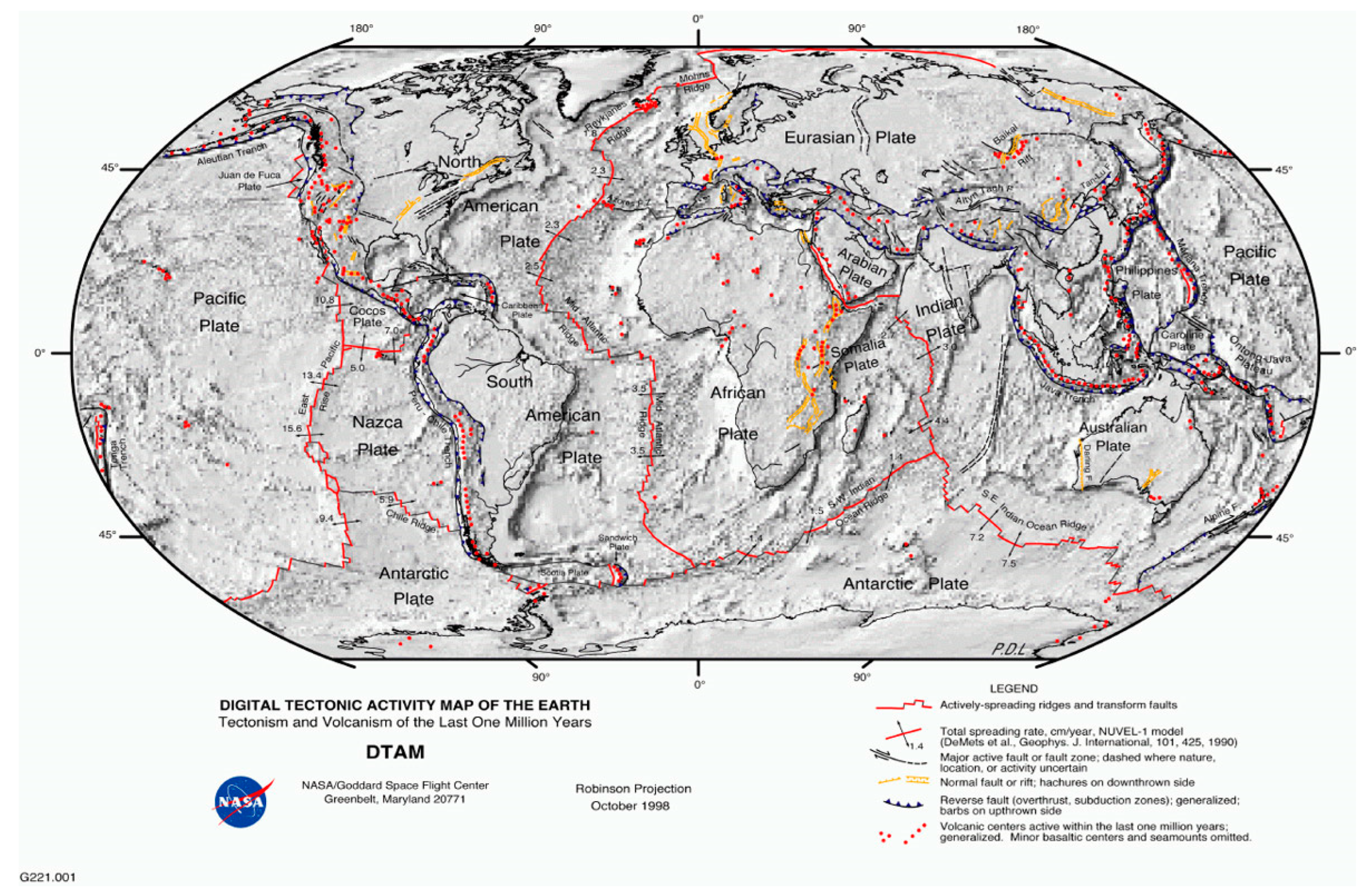
Tectonic plate activity driven by the dynamic processes of the Earth constitutes the primary source of major ground motions, including earthquakes and volcanic eruptions. These activities represent continuous crustal movements that have persisted throughout geological time and are expected to continue for as long as the planet exists. However, the complex and irregular nature of these processes prevents modern science and technology from accurately predicting the exact timing and location of earthquakes. According to plate tectonics theory, the Earth’s lithosphere is divided into several major plates—such as the African, North American, South American, Antarctic, and Australian Plates—as well as numerous smaller plates, including the Scotia, Philippine, and Arabian Plates. The continents situated on these plates are transported passively as the plates move. Although plates are typically named after the continents they carry, their boundaries extend well beyond continental margins into oceanic regions. Consequently, continents undergo spatial displacement as a direct result of underlying plate motions. As illustrated in Figure 1, plate boundaries are the primary loci of tectonic and magmatic activity on Earth, where the largest earthquakes and most intense volcanic eruptions predominantly occur [1].

A substantial portion of deformation within the Earth’s crust is expressed through earthquakes. Quantifying deformation associated with seismic and volcanic processes is a central objective across multiple scientific disciplines, with geodetic methods playing a particularly important role. Modern geodetic measurement technologies provide exceptionally high precision, enabling the detection and monitoring of even small-magnitude deformations in tectonically active regions [3]. Technological advances have reduced operational costs while simultaneously improving measurement accuracy, thereby promoting the widespread use of satellite geodesy in Earth science research. Satellite-based techniques—such as Global Navigation Satellite Systems (GNSS), Interferometric Synthetic Aperture Radar (InSAR), Satellite Laser Ranging (SLR), and Lunar Laser Ranging (LLR)—have largely surpassed traditional terrestrial methods for determining plate motions due to their global coverage, continuity, and high accuracy [4]. The term GNSS denotes the ensemble of global navigation satellite systems operated by different countries. These systems include the United States’ Global Positioning System (GPS), the European Union’s Galileo, Russia’s GLONASS, Japan’s Quasi-Zenith Satellite System (QZSS), China’s BeiDou Navigation Satellite System (BDS), and India’s Indian Regional Navigation Satellite System (IRNSS), among others. GPS represents one of the principal components of the GNSS constellation [5,6].

The concept of integrating GNSS receivers into network-based systems has been implemented since the early 1990s. Advances in telecommunications infrastructure have enabled continuous remote access to GNSS receivers, allowing observation data from numerous stations to be transmitted automatically to processing centers without the need for on-site human intervention. Continuously operating GNSS (CORS) networks that record and transmit data in near real time provide critical information for monitoring tectonic plate motions [7]. High-quality observations obtained from such networks have become a fundamental resource for crustal deformation monitoring, tectonic investigations, the detection of millimeter-scale annual displacements, and the assessment of tectonic strain accumulation [8].

Numerous GNSS networks have been established worldwide to support both regional and international scientific investigations. One of the earliest large-scale networks, Japan’s GPS Earth Observation Network (GEONET), was established in 1993 and comprises more than 1200 GNSS stations, supplemented by several VLBI stations, with an average inter-station spacing of approximately 20 km. GEONET was designed primarily for crustal deformation monitoring and provides real-time data to support earthquake and volcanic research. In Europe, France established the REGAL (Réseau GPS permanent dans les Alpes occidentales) network in 1997 to investigate crustal deformation and estimate strain rates in the Western Alps [9]. In Italy, the Geodetic Data Archiving Facility (GEODAF), operated by the Italian Space Agency at the Centro di Geodesia Spaziale (CGS) in Matera, supplies geodetic data for monitoring tectonic activity across the region. In the United States, additional regional networks include the Southern California Integrated GPS Network (SCIGN) and the Bay Area Regional Deformation (BARD) network in Northern California. Among all regional and national systems, the International GNSS Service (IGS) global network represents the most comprehensive infrastructure for high-precision geodetic applications. Established by the International Association of Geodesy (IAG) in 1993 and operational since 1994, the IGS network provides continuous, high-quality observations from stations distributed worldwide. These data are made available in near real time and archived for public access, supporting a wide range of scientific and geodetic studies [10].

Time series derived from long-term daily observations of permanent GNSS stations contain real-time trends—either linear or nonlinear—as well as periodic variations occurring on semiannual or annual scales. These seasonal effects adversely influence station velocity estimates. Observations from permanent GNSS stations in Antarctica are affected by the region’s harsh environmental conditions and dynamic geophysical processes. Seasonal variations in snow and ice loading cause displacements at the millimeter level in the vertical component, while atmospheric conditions and polar ionospheric variability introduce short-term signal errors. During winter months—particularly throughout the polar night—power shortages, extreme cold, and snow accumulation on antennas may lead to data gaps. In addition, ice sheet motion and seismic events can produce transient deformations at the centimeter level in both horizontal and vertical components. Therefore, Antarctic GNSS time series must be analyzed by carefully accounting for seasonal and transient signals as well as data discontinuities.

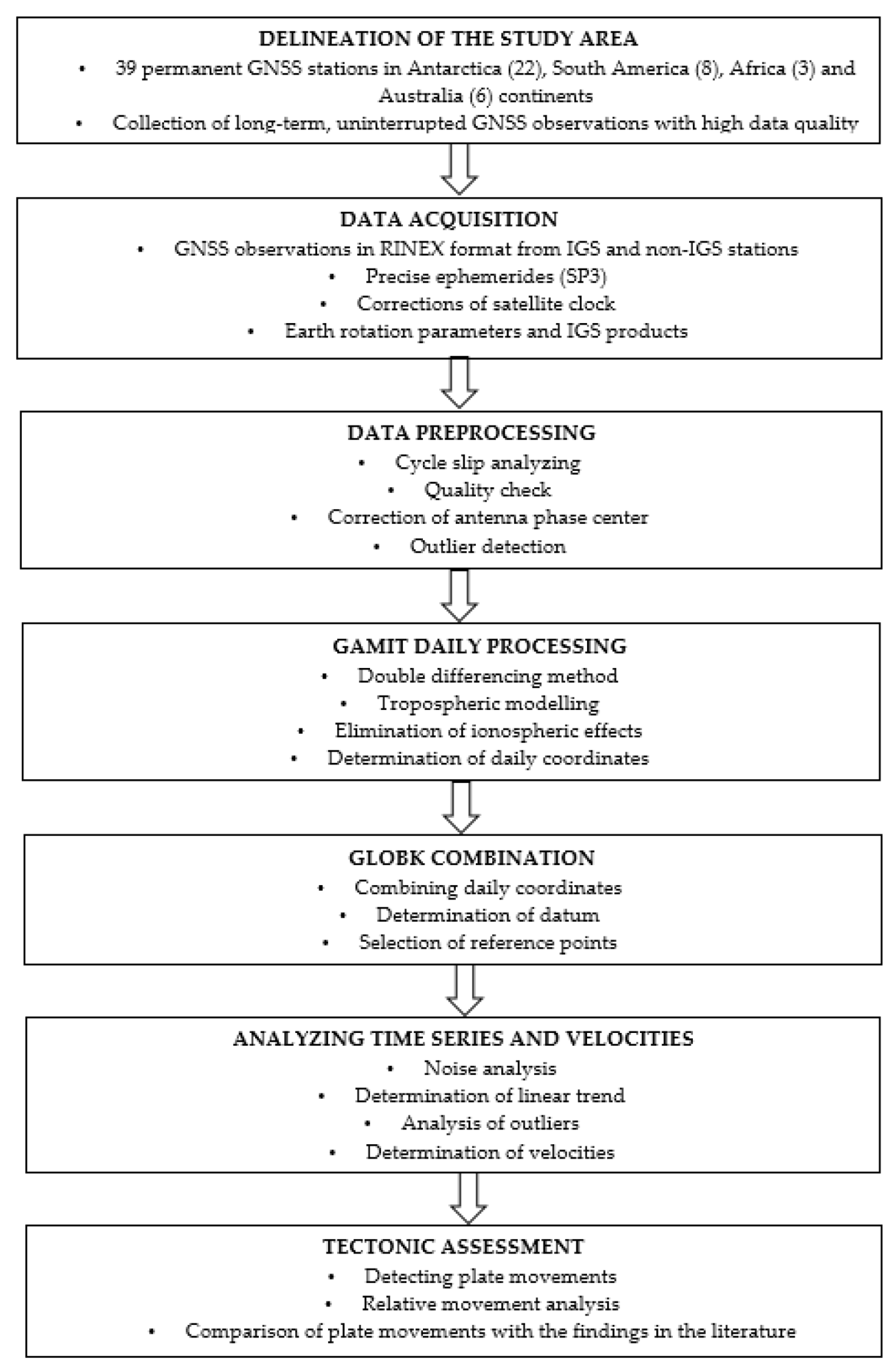
In this study, a geodetic network of 39 stations in Antarctica and neighboring plates has been established. GNSS data collected at these stations between 2020 and 2023 were processed using the GAMIT/GLOBK V10.7 software package to estimate the coordinates and velocities of stations located on the Antarctic, South American, African, and Australian Plates in the ITRF14 reference frame. Furthermore, plate-fixed solutions were generated to analyze the relative motion of the Antarctic Plate with respect to neighboring plates. In Figure 2, a workflow chart for the sequence of research steps is illustrated.

This study focuses on the determination of plate motions using geodetic methods based on data obtained from permanent GNSS stations, with particular emphasis on horizontal movements. Nevertheless, numerous scientific investigations in Antarctica address other research topics like monitoring vertical crustal motions and sea-level variations, GNSS meteorology, and GNSS reflectometry. For example, Hammond et al. [11] examined vertical land motion and global sea-level change, with specific consideration of the Antarctic continent. Hattori et al. [12] estimated glacial isostatic adjustment signals using GNSS observations from Lützow–Holm Bay by applying elastic deformation corrections derived from mass variations observed by the Gravity Recovery and Climate Experiment (GRACE) mission and satellite altimetry. Richter et al. [13] investigated elevation changes in East Antarctica using GNSS data. Selbesoğlu et al. [14] applied the GNSS reflectometry technique to monitor sea level using observations from a permanent GNSS station established on Horseshoe Island as part of Türkiye’s Antarctic research activities. Similarly, Pinat et al. [15] conducted research on long-term variations in snow height in Antarctica using GNSS reflectometry.

2. Materials and Methods

2.1. Study Area

The study area was defined so as to monitor the motions of the Antarctic, South American, Australian and African (Nubian) plates using data obtained from GNSS systems. To this end, it encompasses the entire Antarctic continent, the southern part and western margin of the South American continent, the southernmost tip of the African continent, and the whole of the Australian continent. Antarctica hosts numerous scientific stations operated by different countries, where a broad range of research activities are conducted. Although many of these investigations are concentrated along the western coastal regions of the continent, studies are also carried out on surrounding islands of various sizes. One such location is Horseshoe Island, part of the Faure Islands group, where Turkish scientists conduct research at a temporary station established within the framework of the Turkish Antarctic Scientific Expeditions.

The main reason for including the southern part of South America in this study is its proximity to the Antarctic continent, particularly the Chilean sector, which allows a better observation of the relative motion between the South American and Antarctic plates in this region. In addition, the western margin of the continent was incorporated into the study in order to monitor the motion of the Nazca Plate along the Pacific plate boundary zone.

To investigate the relationship between the African (Nubian) Plate and the adjacent Antarctic Plate, three GNSS stations belonging to the IGS network and located at the southern tip of the African continent were included in the study area. The African Plate is generally regarded as tectonically stable compared with neighboring plates. Therefore, selecting three stations located in the southern part of the continent, in proximity to Antarctica, was considered sufficient to represent the plate’s motion within the study area.

The Australian Plate, which also borders the Antarctic Plate, was included in the study because it is one of the most seismically active and kinematically fastest-moving plates on Earth. Accordingly, continuous GNSS stations distributed across the Australian continent were incorporated into the analyses.

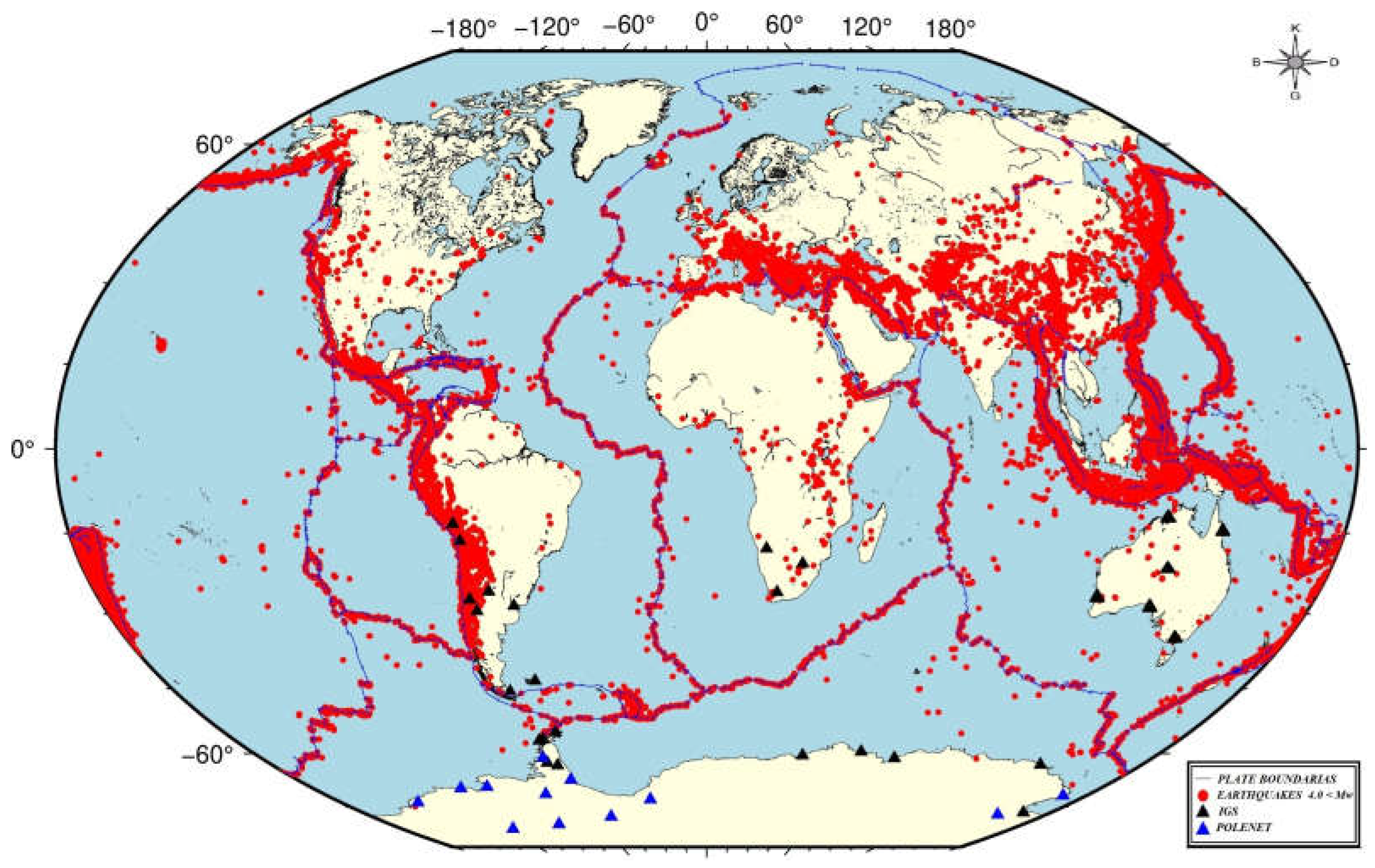
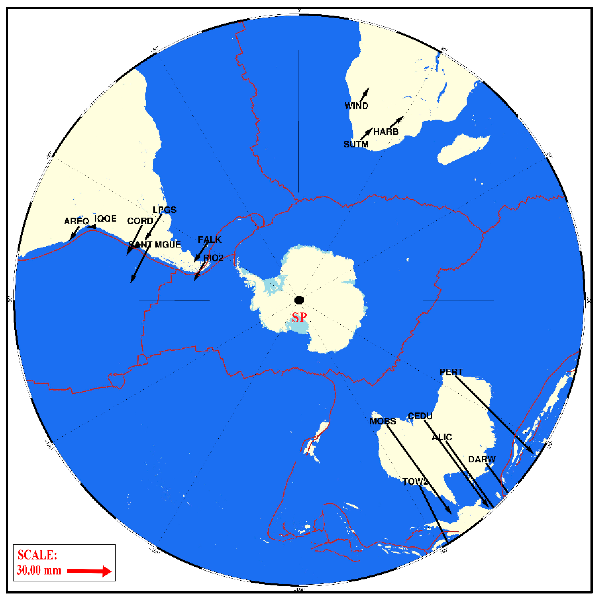
The stations in the research area include existing IGS stations and POLENET network points operating with more than 100 permanent GNSS stations on the Antarctic continent. In total, the network consists of 39 permanent GNSS stations: 22 on the Antarctic Plate, 8 on the South American Plate, 6 on the Australian Plate, and 3 on the African Plate. The distribution of these stations within the study area is shown in Figure 3. In selecting stations, several factors were taken into account, including continuity of measurements, multipath conditions, monument stability, the ability of the station to reliably represent the motion of the tectonic plate on which it is located, and the suitability of its position with respect to the geometry of plate boundaries. Although continuity of measurements was considered, data gaps are present in some of the stations in Antarctica, particularly in the periods corresponding to the polar night. Information on the stations used in the research is given in

Table 1. Station information of the GNSS networks used.

Point Number	Station Name	Station ID	Latitude (°)	Longitude (°)	Ell. Height (m)	Network
1	Arequipa, Peru	AREQ	16.46552 S	71.4928 W	2488.928	IGS
2	McMurdo Station, Antarctica	ARHT	77.82944 S	166.66366 E	135.3350	IGS
3	Cordoba, Argentina	CORD	31.52843 S	64.47005 W	746.8335	IGS
4	Davis, Antarctica	DAV1	68.57732 S	77.97261 E	44.3875	IGS
5	Dumont d’Urville, Antarctica	DUMG	66.66519 S	140.00219 E	−1.6427	IGS
6	Falkland Island (Malvinas)	FALK	51.69365 S	57.87407 W	50.8197	IGS
7	Pretoria, South Africa	HARB	25.88696 S	27.70725 E	1558.085	IGS
8	Hugo Island, Antarctica	HUGO	64.96256 S	65.66754 W	20.6361	IGS
9	Iquique, Chile	IQQE	20.27354 S	70.13172 W	38.9717	IGS
10	La Plata, Argentina	LPGS	34.90674 S	57.9323 W	29.8670	IGS
11	Mawson, Antarctica	MAW1	67.60477 S	62.87071 E	59.1171	IGS
12	Malargue, Argentina	MGUE	35.77735 S	69.39793 W	1553.717	IGS
13	O’Higgins, Antarctica	OHI3	63.32109 S	57.90138 E	32.6362	IGS
14	Palmer Station, Antarctica	PALM	64.77509 S	64.05112 W	31.1391	IGS
15	Rio Grande, Argentina	RIO2	53.78547 S	67.75112 W	32.0237	IGS
16	Santiago, Chile	SANT	33.15029 S	70.66855 W	723.1162	IGS
17	Sutherland, Güney Afrika	SUTM	32.38143 S	20.81091 E	1797.618	IGS
18	East Ongle Island, Antarctica Antarctica	SYOG	69.00696 S	39.58374 E	49.9921	IGS
19	Traverse Mountains, Antarctica	TRVE	69.98882 S	67.55471 W	1064.349	IGS
20	Windhoek, Namibia	WIND	22.57492 S	17.08944 E	1734.681	IGS
21	Welch Mountains, Antarctica	WLCH	70.72935 S	63.82041 W	1534.123	IGS
22	Alice Springs Australia	ALIC	23.67011 S	133.88552 E	603.2343	IGS
23	Ceduna, Australia	CEDU	31.86666 S	133.80984 E	144.7163	IGS
24	Darwin, Australia	DARW	12.84370 S	131.13274 E	125.1024	IGS
25	Melbourne, Australia	MOBS	37.82940 S	144.97534 E	40.5640	IGS
26	Perth, Australia	PERT	31.80196 S	115.88526 E	12.6656	IGS
27	Townsville, Australia	TOW2	19.26927 S	147.05569 E	88.0936	IGS
28	Backer Island, Antarctica	BACK	74.43044 S	102.47818W	33.3562	POLENET
29	Bennett Nunatak, Antarctica	BENN	84.78646 S	116.45979W	1416.46	POLENET
30	Butcher Ridge, Antarctica	BURI	79.14744 S	155.89416 E	2006.309	POLENET
31	Cordiner Peak, Antarctica	CRDI	82.86152 S	53.19913 W	945.3200	POLENET
32	Haag Nunatak, Antarctica	HAAG	77.03805 S	78.28711 W	1171.809	POLENET
33	Hutton Mountains, Antarctica	HTON	74.08001 S	61.73059 W	950.4719	POLENET
34	Mt Carbone, Antarctica	MCAR	76.3222 S	144.30351W	964.8968	POLENET
35	Martin_Peninsula, Antarctica	MRTP	74.1804 S	115.10213W	96.4097	POLENET
36	Stewart Hills, Antarctica	STEW	84.18701 S	86.24729 W	1587.0520	POLENET
37	Theron Mountains, Antarctica	THRO	79.12669 S	28.31891 W	1058.1350	POLENET
38	Tombstone Hill, Antarctica	VL01	72.45014 S	169.72508 E	596.8925	POLENET
39	Dismal Island, Antarctica	DISM	68.09113 S	68.84476 W	37.3392	DGM

.

In this study, 24 h observations from these stations covering the period 2020–2023 have been processed and analyzed. As in Figure 3, the visualization of station locations and graphical representation of station motions relative to the plates on which they are situated were conducted using the Generic Mapping Tools (GMT) V.6.4.0 software package [16]. These visualizations were produced using open-access data provided by the U.S. Geological Survey (USGS), the National Science Foundation (NSF), and EarthScope [17,18,19].

2.2. Evaluation of GNSS Observations and Estimation of GNSS Station Velocities

GNSS receivers record 24 h observations as raw data in proprietary formats specific to each receiver model. Before the analysis, the raw data must be converted into the Receiver Independent Exchange Format (RINEX), which is the international standard exchange format. For this purpose, each receiver manufacturer provides conversion utilities, enabling observation data to be transformed into RINEX format with relative ease. At present, a wide variety of software packages are employed for the analysis of GNSS data, serving different objectives. These include scientific and educational software such as GAMIT/GLOBK, BERNESE, GIPSY-OASIS, GEONAP and MICROCOSM, as well as commercially developed platforms such as Trimble Pivot Platform (TPP), TopNET+, GNSS Spider, Leica Geo Office and Leica Infinity.

In this study, the GAMIT/GLOBK V.10.7 software, a comprehensive scientific package developed by the Massachusetts Institute of Technology (MIT) for analyzing GNSS observations to determine crustal deformation, was employed [20]. The software consists of two main modules. The GAMIT (GNSS at MIT) module is a collection of programs that process phase observations in order to estimate the three-dimensional relative positions of ground stations and satellite orbits, atmospheric zenith delays, and Earth orientation parameters. The primary purpose of the GLOBK (Global Kalman Filter) module is to combine different geodetic solutions. As input, it accepts station coordinates, Earth orientation parameters, orbit parameters, and source positions, along with their covariance matrices, obtained from the analysis of primary observations. These individual solutions are typically generated by assigning large a priori uncertainties to global parameters, so that constraints can be applied uniformly in the combined solution [21].

In accordance with the adopted GNSS processing strategy given in

Table 2. GNSS data processing strategy information.

Processing Strategy
Data sampling rate	30 s
Satellite elevation cut-off angle	0°
Orbit information	IGS-Final
Earth rotation parameters	USNO_bull_b
Earth orientation model	TUME1
Number of iterations for solution	1
Tropospheric Model	VMF1 (Vienna Mapping Function-1)
Carrier Wave Phase Ambiguity Resolution	Ionosphere-free

, the 24 h RINEX data were initially subjected to quality control using the Translation, Editing, and Quality Check (TEQC) software in order to assess multipath effects and observation quality [22].

In the GLOBK analysis stage, a number of programs such as glred, globk and glorg are used. First, the glred program is executed to combine the daily H-files produced by the GAMIT processing and to map them into a given reference frame, thereby generating time series for each station. In this way, both long- and short-term time series can be obtained for all stations. The daily combined H-files are then merged on a monthly basis to produce a single H-file representing longer time spans. This procedure is carried out using the GLOBK submodule. The glorg module is used for the realization of the reference frame and for the estimation of station velocities. In GLOBK, observations acquired at different epochs are combined using the Kalman filtering technique. Through this combination, a strategy is implemented to estimate both station coordinates and velocities. Discontinuities caused by antenna and receiver changes, as well as earthquake-related offsets, were introduced into the model via the eq_file and solved as step parameters. Kinematic models are employed to understand geodynamic processes; these models describe positional changes over time and involve the application of various filtering techniques. Filtering procedures are used to predict the state of the system, reduce data noise, and optimally combine observations [23]. The Kalman filter, also known as the Kalman–Bucy filter and in use since 1960, can be summarized as a recursive prediction–correction algorithm [24]. Following the GLOBK solution, the resulting coordinate time series are re-modeled using the TSFIT program, in which linear trends, seasonal components, and defined offsets are estimated simultaneously. Velocity uncertainties are recomputed by considering both white noise and time-correlated noise components.

Prior to the final estimation of precise positions and velocities, the time series were examined to assess whether the results for each station were suitable for tectonic interpretation and for evaluating data quality. The daily time series produced for stations with long observation intervals provide insight into their overall tectonic behavior. Because the Kalman filter propagates modeling and solution errors throughout the entire time series, the series were carefully inspected and interpreted. Time series for all stations were plotted, and outlying observations were removed from the analyses. During the daily and monthly combination steps, the list of reference stations defined within the glorg.cmd file was used for the specification of the reference frame. For geophysical interpretation, it is natural to express the derived velocities in a reference frame tied to a stable tectonic block, typically corresponding to a major plate in the vicinity of the network. When a primary plate realization based on the ITRF dataset is desired [25], transformed ITRF a priori files (e.g., igb14_noam.apr) provided in the gg/tables directory are specified in the glorg.cmd file. In this manner, a rotation vector (Euler pole) is estimated for a block encompassing the region of interest with respect to the stabilization frame. These plate a priori files contain the rotation vector velocities for each station. The glorg output file reports the components and uncertainties of the estimated rotation vector, as well as the velocity adjustments relative to the a priori file, effectively transforming the velocities into a frame fixed to the selected plate. Any number of plates can be estimated in a single solution, provided the corresponding station sets are independent and do not substantially overlap the areas used for stabilization. The sh_org2vel command is then run with the glorg output and plate files as input to generate a velocity summary that contains the motions of all sites in the solution with respect to each plate [20].

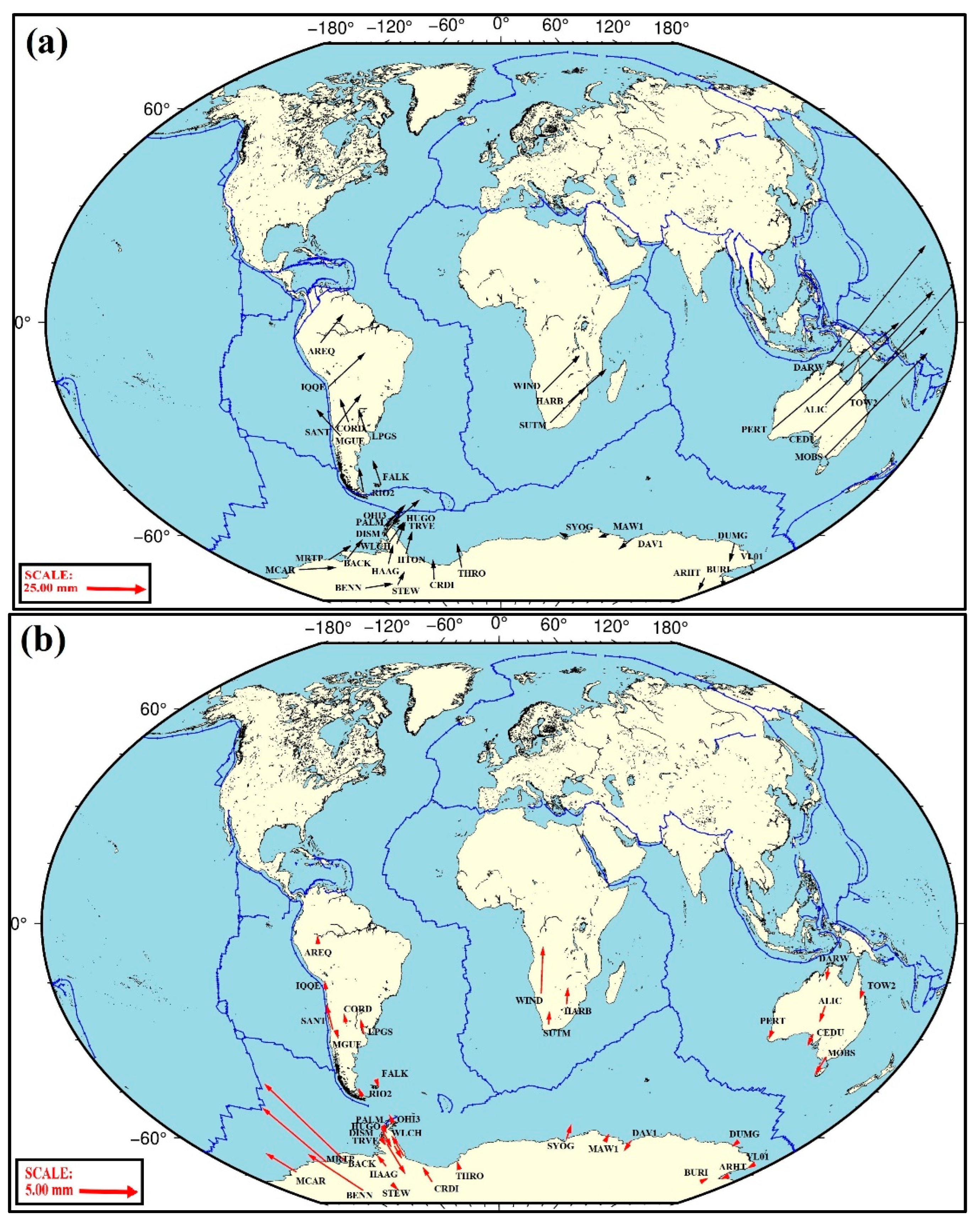
Following the final position and velocity estimations, the summary of station velocities can be obtained from the “SUMMARY VELOCITY ESTIMATES FROM GLOBK Ver 5.34X” section of the file globk_vel.org. The velocity and position estimates for the stations derived from the analyses are presented in

Table 3. Summary of velocity and position estimates of stations.

Site	N Rate (mm/year)	E Rate (mm/year)	h Rate (mm/year)	N± (mm/year)	E± (mm/year)	h± (mm/year)	dE± (mm/year)	dN± (mm/year)	dh± (mm/year)
ALIC *	59.46	31.75	−2.62	0.04	0.04	0.26	0.06	0.08	0.45
AREQ *	13.46	11.33	1.37	0.05	0.04	0.20	0.08	0.09	0.44
ARHT *	−10.46	10.00	−0.11	0.04	0.04	0.19	0.07	0.07	0.33
BACK	11.31	15.30	17.59	0.07	0.06	0.20	0.13	0.14	0.53
BENN	2.39	14.97	10.39	0.05	0.05	0.20	0.10	0.10	0.50
BURI	−11.37	7.10	0.79	0.07	0.06	0.29	0.11	0.13	0.53
CEDU *	58.11	28.96	−2.02	0.04	0.05	0.20	0.07	0.08	0.35
CORD	11.45	−1.68	1.62	0.06	0.06	0.20	0.11	0.12	0.40
CRDI	11.05	5.26	2.72	0.06	0.05	0.20	0.09	0.10	0.49
DARW	59.81	35.37	−1.90	0.10	0.10	0.42	0.19	0.18	0.77
DAV1	−6.38	−2.88	−1.95	0.08	0.06	0.26	0.11	0.14	0.46
DISM	10.88	12.88	−1.23	0.15	0.12	0.50	0.28	0.34	1.14
DUMG	−12.43	7.58	−0.29	0.09	0.07	0.30	0.14	0.17	0.55
FALK *	12.25	0.06	−0.12	0.06	0.05	0.20	0.09	0.11	0.40
HAAG	10.94	9.18	2.20	0.07	0.06	0.20	0.11	0.12	0.50
HARB	16.15	16.90	2.62	0.12	0.12	0.28	0.22	0.22	0.50
HTON	11.79	8.91	3.68	0.06	0.05	0.20	0.09	0.10	0.38
HUGO	9.02	13.13	−3.29	0.08	0.06	0.20	0.12	0.14	0.44
IQQE	15.83	19.68	1.20	0.07	0.07	0.20	0.13	0.12	0.49
LPGS *	11.42	−1.43	2.34	0.16	0.16	0.69	0.18	0.18	0.75
MAW1 *	−2.18	−4.31	0.40	0.06	0.04	0.21	0.07	0.10	0.37
MCAR	−1.76	16.19	5.62	0.06	0.06	0.23	0.11	0.11	0.41
MGUE *	13.39	−7.99	−0.09	0.07	0.06	0.20	0.11	0.12	0.40
MOBS	59.81	15.72	−3.27	0.06	0.07	0.23	0.11	0.13	0.42
MRTP	8.01	16.70	13.22	0.08	0.07	0.30	0.13	0.15	0.54
OHI3 *	10.01	15.70	1.36	0.06	0.05	0.20	0.09	0.11	0.39
PALM *	10.36	13.68	−0.94	0.05	0.04	0.10	0.09	0.10	0.31
PERT *	57.59	38.43	−1.40	0.08	0.08	0.30	0.14	0.14	0.54
RIO2	12.44	2.69	1.00	0.05	0.06	0.18	0.09	0.11	0.32
SANT *	15.60	15.98	4.01	0.05	0.04	0.10	0.08	0.09	0.33
STEW	8.63	9.57	−0.59	0.08	0.07	0.40	0.13	0.14	0.75
SUTM	17.11	15.79	2.06	0.11	0.11	0.25	0.19	0.19	0.45
SYOG *	1.97	−4.78	2.42	0.07	0.06	0.25	0.09	0.10	0.38
THRO	11.72	1.32	1.38	0.06	0.06	0.20	0.12	0.13	0.57
TOW2	57.24	28.13	−1.05	0.08	0.07	0.29	0.14	0.12	0.50
TRVE	10.32	12.22	−5.50	0.09	0.07	0.20	0.10	0.11	0.37
VL01	−10.08	12.38	−0.35	0.07	0.07	0.26	0.12	0.14	0.48
WIND	17.52	16.77	7.39	0.12	0.13	0.30	0.23	0.23	0.52
WLCH	11.31	9.66	−2.27	0.07	0.05	0.20	0.09	0.10	0.33

N & E Rate: Velocities (mm/year) in the topocentric north and east components in the ITRF14 (igb14) reference frame. h Rate: Velocity of ellipsoidal height (mm/year). N & E±: Standard deviations (sigma) of the east and north velocity components. h±: Standard deviation (sigma) of the ellipsoidal height rate. dE & dN ±: Standard deviations (sigma) of the east and north coordinate components in the horizontal plane. dh±: Standard deviation (sigma) of the ellipsoidal height. * indicates the points used for the definition of the reference frame.

. Based on these values, the ITRF14 horizontal and vertical position–velocity components of the stations are illustrated in Figure 4a and Figure 4b, respectively.

For stations whose velocities are to be expressed in a different reference frame, such as EUREF, it is sufficient to rerun only the glorg module with the appropriate a priori files. Reference frame files for various plates are available in the tables subdirectory of the GAMIT/GLOBK installation. In this study, the following plate models were used: South American Plate (igb14_comb_soam.apr), African Plate (igb14_comb_nubi.apr), Antarctic Plate (igb14_comb_anta.apr) and Australian Plate (igb14_comb_aust.apr). By fixing each of the four plates within the study area in turn, the position–velocity information describing the motion of neighboring plates was obtained; a summary of these plate-fixed velocity solutions is given in

Table 4. Summary of velocities of plate fixed solutions in the ITRF14 reference frame.

Australian Plate Fixed		South American Plate Fixed		Antarctic Plate Fixed		African Plate Fixed		SITE
N Rate (mm/year)	E Rate (mm/year)	N Rate (mm/year)	E Rate (mm/year)	N Rate (mm/year)	E Rate (mm/year)	N Rate (mm/year)	E Rate (mm/year)
69.42	−19.57	2.58	13.75	3.01	−10.69	10.33	−15.76	AREQ
−56.50	38.26	0.48	5.10	1.03	0.57	7.26	12.38	ARHT
69.49	−27.14	−0.09	−0.48	0.23	−22.48	6.04	−30.61	CORD
−44.40	−58.13	−0.17	8.76	−0.97	0.05	−13.30	5.45	DAV1
67.17	15.35	−0.23	9.26	0.15	−1.01	6.90	−12.99	DISM
−70.28	4.51	0.03	8.92	0.16	−0.21	0.13	11.88	DUMG
71.25	−18.38	0.25	0.06	0.46	−16.35	4.77	−27.85	FALK
27.06	−40.82	11.81	25.89	10.86	3.10	−2.07	−0.82	HARB
66.44	10.12	−2.39	10.41	−2.06	−1.12	4.01	−13.25	HUGO
72.26	−9.51	4.81	21.71	5.22	−2.26	12.25	−8.10	IQQE
70.56	−28.85	−0.59	0.16	−0.38	−21.08	3.95	−30.11	LPGS
−26.95	−67.63	0.99	8.48	0.08	−0.85	−13.52	1.31	MAW1
70.03	−28.16	2.30	−7.83	2.70	−28.83	9.58	−37.36	MGUE
68.99	4.47	−1.97	14.58	−1.77	2.37	2.55	−10.27	OHI3
68.25	9.02	−1.19	11.28	−0.89	−0.33	4.83	−12.60	PALM
69.53	−6.47	1.21	0.87	1.58	−14.79	8.10	−25.78	RIO2
71.80	−5.22	4.65	16.34	5.06	−5.28	12.21	−13.31	SANT
34.86	−45.04	11.40	25.37	10.49	3.88	−1.71	−1.27	SUTM
0.17	−72.71	0.12	8.27	−0.85	−0.84	−14.56	−3.86	SYOG
67.21	14.12	−0.91	8.63	−0.56	−0.88	5.93	−13.09	TRVE
39.20	−37.88	11.09	24.86	10.2	1.43	−1.53	−3.12	WIND
69.22	8.81	−0.26	6.70	0.04	−2.53	5.70	−15.15	WLCH
48.86	49.33	5.19	6.01	6.01	−1.31	18.39	−7.97	BACK
27.84	64.81	−0.93	3.40	−0.01	0.76	13.56	−2.62	BENN
−63.70	27.39	0.49	4.18	0.88	0.30	4.67	13.14	BURI
70.33	1.96	−1.16	3.37	−1.05	−0.74	2.16	−14.42	CRDI
64.08	26.47	0.91	2.95	1.43	−3.54	10.10	−14.58	HAAG
70.12	8.38	0.06	6.03	0.32	−1.81	5.52	−14.75	HTON
−4.15	64.93	0.92	5.40	1.90	−0.46	15.41	2.49	MCAR
34.92	57.49	4.41	6.41	5.33	−0.84	18.82	−4.74	MRTP
57.43	38.94	−0.28	1.34	0.34	−1.98	10.44	−11.73	STEW
65.87	−28.9	−0.39	5.01	−0.70	−0.67	−3.49	−14.43	THRO
−54.13	38.86	0.53	7.47	1.13	0.59	8.02	11.61	VL01
0.51	−0.27	71.92	36.09	71.93	13.38	70.42	17.28	ALIC
−0.81	0.14	70.56	33.13	70.58	12.22	69.05	17.99	CEDU
0.60	−0.56	72.22	39.92	72.16	15.56	69.99	16.86	DRAW
3.20	−3.46	72.21	18.24	72.41	−1.11	73.60	5.97	MOBS
−0.33	−0.08	69.16	44.59	68.87	23.64	63.14	28.81	PERT
1.23	−1.01	69.58	31.58	69.81	8.09	71.51	10.94	TOW2

within the ITRF14 reference frame.

3. Results

3.1. African Plate

The African Plate consists of several smaller plates, most notably the Somali and Arabian Plates. With an area of approximately 61,334,000 km², it is the fourth largest tectonic plate on Earth. The African Plate is largely bordered by oceanic crust along its western and southern margins, except for its easternmost part. It is bounded to the west by the South and North American Plates, to the north by the Eurasian and Aegean–Anatolian Plates, to the east by the Arabian–Somali Plates, and to the south by the Antarctic Plate. The kinematics of the African Plate is complex, involving both convergent and divergent motions and incorporating a variety of fault systems.

Geodynamic investigations in this region attract considerable scientific interest, as they have the potential to provide a more detailed understanding of the processes occurring within the African Plate system. In many recent studies, GNSS techniques have been preferred because they enable the investigation of spatial displacements with high accuracy. There are numerous examples of the use of these techniques in the geodynamic investigation of different parts of the African Plate system [26,27,28,29,30]. Reported horizontal velocities generally fall within the range of 20–60 mm/year and differ across the various regions of the African Plate system. Savchyn [31] derived horizontal velocities in the ITRF14 reference frame for permanent GNSS stations located on the African Plate for the period 1996–2022. Their results indicate a northeastward motion with magnitudes between 18.8 and 47.8 mm/year.

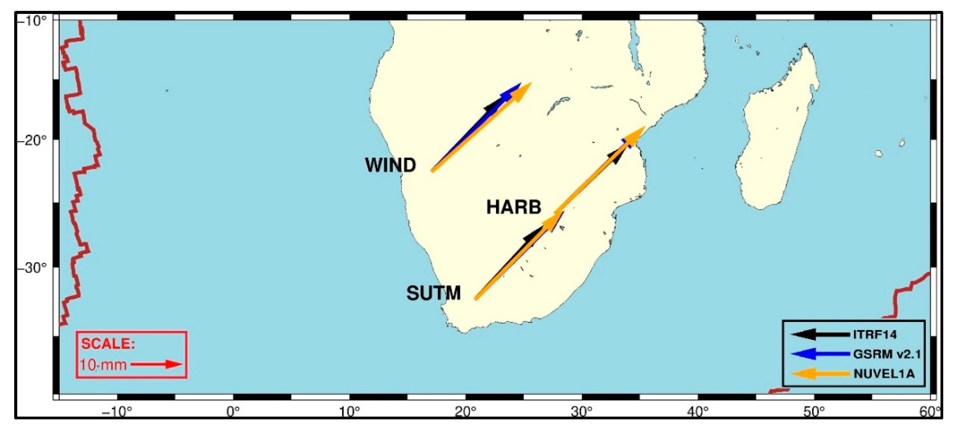
Within the African Plate system, the velocities of the WIND, HARB and SUTM continuous GNSS stations located in the study area, expressed in the ITRF14 reference frame, are found to be approximately 23–24 mm/year in a northeastward direction. To assess the reliability of these estimates, the GNSS-derived velocities were compared with the GSRM v2.1 (Global Strain Rate Map) and NUVEL-1A plate motion models. In addition to these three models, the horizontal velocity components obtained from analyses by the Nevada Geodetic Laboratory and the Jet Propulsion Laboratory of the California Institute of Technology were compiled and are listed in

Table 5. Velocities of African Plate GNSS stations in different plate models.

Station Name	ITRF14 Plate Model		GSRM v2.1 Plate Model		NUVEL-1A Plate Model		Nevada Geodesy Laboratory		California Institute of Technology Jet Propulsion Lab.
	N Rate (mm/year)	E Rate (mm/year)	N Rate (mm/year)	N Rate (mm/year)	N Rate (mm/year)	E Rate (mm/year)	N Rate (mm/year)	E Rate (mm/year)	N Rate (mm/year)	E Rate (mm/year)
HARB	16.15	16.90	19.78	20.13	20.13	20.71	18.48	17.71	18.57	17.70
SUTM	17.11	15.79	20.30	20.48	20.48	20.23	19.24	16.72	19.26	16.81
WIND	17.52	16.77	20.47	20.55	20.55	22.97	19.43	19.40	19.08	19.83

; the agreement among the different models is illustrated in Figure 5.

The GSRM v2.1 and NUVEL-1A models are commonly used global plate motion models. The GSRM v2.1 model provides rotational parameters for 50 plates (major and minor) and models the deformation field within plate boundary zones. It constrains the motions of several plates more tightly than previous geodetic plate motion models and is based exclusively on Global Navigation Satellite Systems data (i.e., without using VLBI or DORIS), for the period 1996–2013. The NUVEL-1A model, on the other hand, describes the relative motion rates and directions of the major tectonic plates on Earth. It is constructed from multiple data sources, including geodetic observations, GPS measurements, seafloor spreading data and geological evidence, thus yielding precise and reliable information on plate motions. This model is also used by the IERS. NUVEL-1A is primarily based on magnetic seafloor spreading anomalies over the last ~3 million years and only includes rigid plates. An alternative approach is to construct an Actual Plate Kinematic and Deformation Model (APKIM) from modern space-geodetic observations, including VLBI, SLR and GPS [32]. Both GSRM v2.1 and NUVEL-1A are global models derived for different time periods and using different datasets, which allows comparisons between our solutions and models based on varying temporal and methodological frameworks. Using the Plate Motion Calculator developed by UNAVCO, the east and north velocity components for the HARB, SUTM and WIND stations were computed from both plate motion models and compared with the ITRF14-based velocities obtained from our GAMIT/GLOBK solutions. The results show consistency at the level of 3–4 mm. Furthermore, comparison with the Nevada Geodetic Laboratory and Jet Propulsion Laboratory solutions reveals agreement within 1–3 mm.

3.2. South American Plate

The South American Plate covers an area of approximately 43,000,000 km² and comprises the entire South American continent as well as the surrounding oceanic basins. As shown in Figure 1, it is bounded to the west by the Nazca Plate, to the east by the African Plate along the mid-Atlantic region, to the north by the Caribbean Plate, and to the south by the Antarctic Plate. The westward motion of the South American Plate and its collision with the Nazca Plate has led to the uplift of the Andes. This subduction process is accompanied by intense volcanic and seismic activity. Many of the world’s largest earthquakes occur along this convergent margin. To the east, along its boundary with the African Plate, spreading at the Mid-Atlantic Ridge causes the Atlantic Ocean to widen, forming seafloor troughs and ridges. To the south, the plate boundary with the Antarctic Plate is characterized by a transform-type margin.

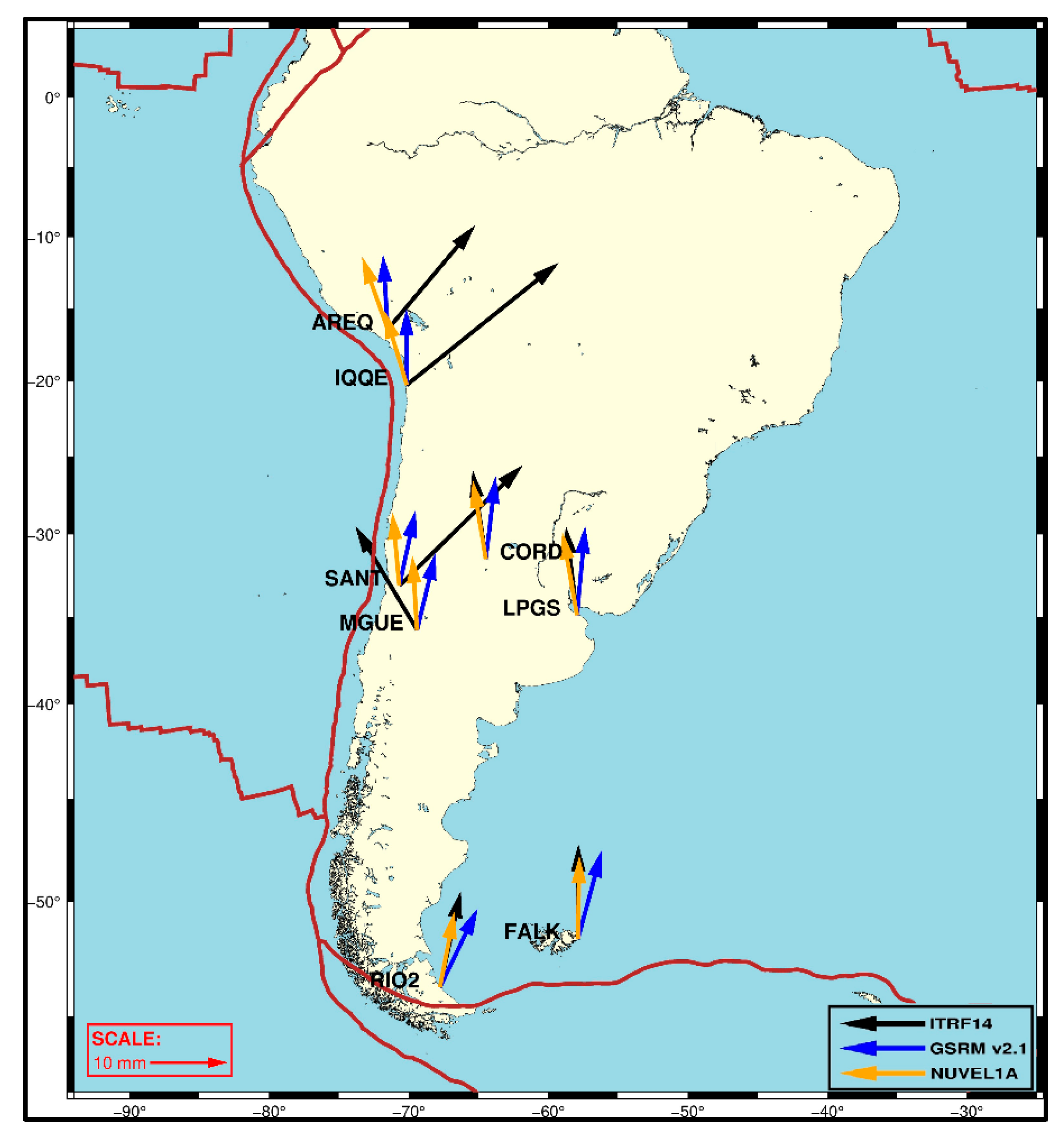
To monitor crustal deformation and plate motion in the seismically and volcanically active South American Plate, a dense network of permanent GNSS stations (IGS) has been established across the continent. For the purposes of this study, eight stations—most of which are situated along the Andean belt—were selected and incorporated into the analysis. Examination of the horizontal displacements of these stations in the ITRF14/IGB14 reference frame reveals that stations located on the western flank of the Andes exhibit velocities of 17–24 mm/year toward the northeast, whereas stations situated on the eastern side show velocities of 6–15 mm/year directed toward the northwest. To further evaluate our solutions, the station velocities were compared with the NUVEL-1A and GSRM v2.1 plate motion models. The comparisons given in

Table 6. Velocities of South American plate GNSS stations in different plate models.

Station Name	ITRF14 Plate Model		GSRM v2.1 Plate Model		NUVEL-1A Plate Model
	N Rate (mm/year)	E Rate (mm/year)	N Rate (mm/year)	E Rate (mm/year)	N Rate (mm/year)	E Rate (mm/year)
AREQ	13.46	11.33	9.62	−0.62	9.34	−3.33
IQQE	15.83	19.68	9.83	−0.05	9.51	−2.85
SANT	15.60	15.98	9.74	2.11	9.44	−0.88
MGUE	13.39	−7.99	9.94	2.41	9.59	−0.60
LPGS	11.42	−1.43	11.49	1.05	10.73	−1.90
CORD	11.45	−1.68	10.66	1.27	10.13	−1.68
FALK	12.25	0.06	11.49	3.12	10.72	0.20
RIO2	12.44	2.69	10.18	4.87	9.76	1.88

indicate that significant discrepancies exist for stations AREQ, IQQE, SANT and MGUE, particularly on the western flank of the Andes. By contrast, the LPGS, CORD, FALK and RIO2 stations agree with the global models to within approximately 5 mm/year. For AREQ, IQQE, SANT and MGUE, however, differences of about 9–19 mm/year are observed, as illustrated in Figure 6.

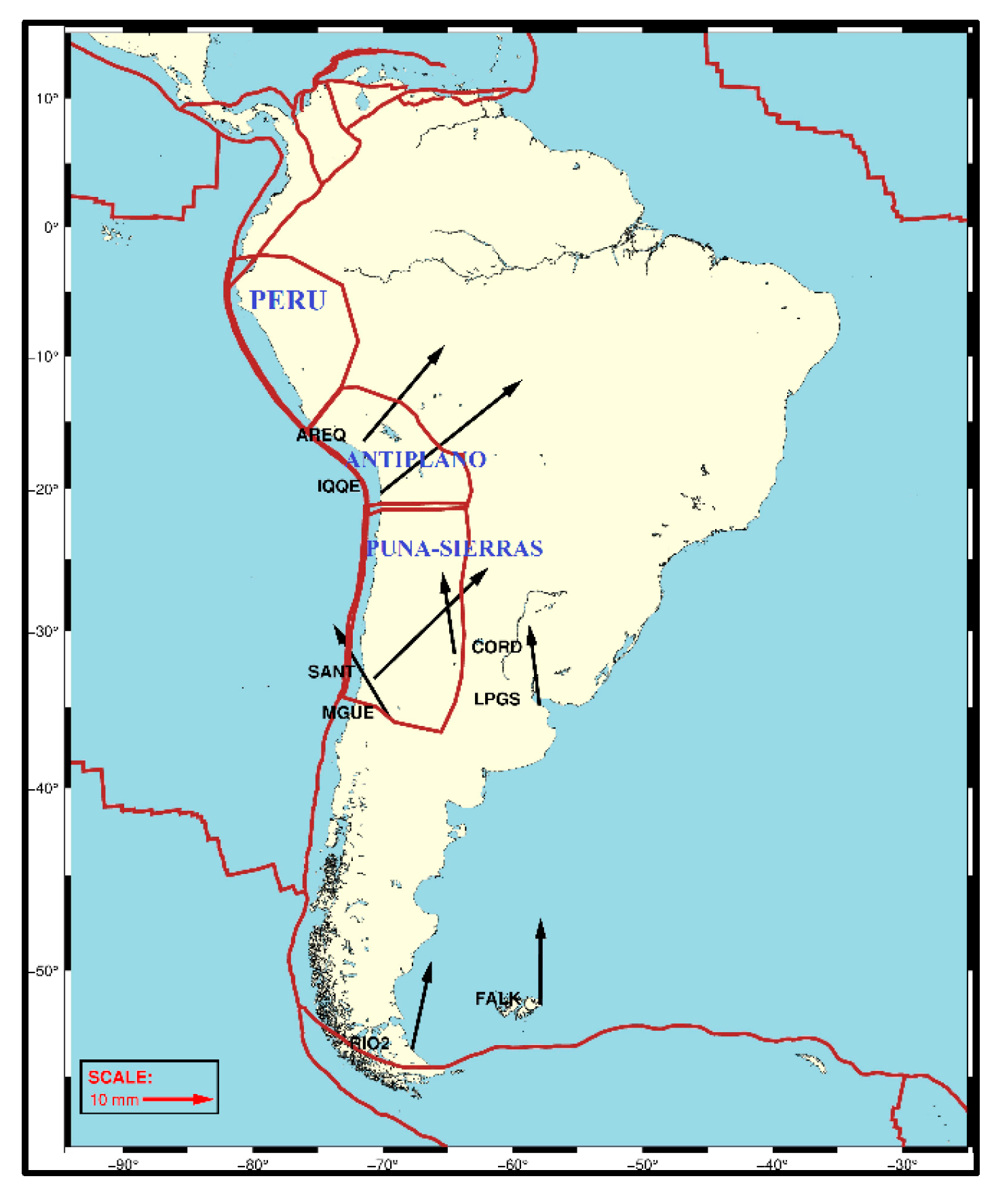
The region extending across Peru, Chile and Argentina is known to be among the most seismically and volcanically active areas on Earth. The South American arc spans a distance of roughly 7000 km, extending from the Chile triple junction off the southern coast of Chile to the intersection with the Panama fracture zone in Central America. This arc delineates the boundary where the Nazca Plate subducts beneath the South American Plate and marks the onset of descent of the Nazca oceanic crust and lithosphere into the mantle beneath South America. The convergence associated with this subduction process is responsible for the uplift of the Andes and for the development of an active volcanic chain in front of the deforming margin. Since 1900, numerous great earthquakes (Mw ≥ 8) have occurred along this subduction interface, many of which have generated devastating tsunamis. Hayes et al. [33] identified five major subduction segments along the Nazca–South America plate boundary based on their study of earthquakes in the region. Two of these segments, the southern Peru and central Chile subduction zones, coincide with the locations of stations AREQ, IQQE, SANT and MGUE used in this study. The presence of these multiple subduction segments has led to the development of small microplates in the region. These microplates are shown in Figure 1 in Gutscher et al. 1999 [34]. Along the western margin of South America, these microplates include the Peru, Altiplano and Puna–Sierras Pampeanas blocks, within which our stations are situated. The spatial relationship between the stations and these microplates is shown in Figure 7.

Since the ITRF14, GSRM v2.1 and NUVEL-1A models are global plate motion models and because many large earthquakes have occurred in this region—especially in the areas comprising the three microplates—between the time periods covered by these models and the present, discrepancies between our GNSS-derived velocities and the model predictions are not unexpected. Major earthquakes in this region include, among others, the Arequipa (Mw 8.4, June 2001), Maule (Mw 8.8, February 2010), Nicoya (Mw 7.6, September 2012), Champerico (Mw 7.4, November 2012), Pisagua–Iquique (Mw 8.2, April 2014), Illapel (Mw 8.3, September 2015), Pedernales (Mw 7.8, April 2016), Quellón (Mw 7.6, December 2016), Atiquipa (Mw 7.1, January 2018), Palora (Mw 7.5, February 2019), Navarro (Mw 8.0, May 2019), Barranca (Mw 7.5, November 2021) and Azángaro (Mw 7.2, May 2022) earthquakes. These earthquakes contribute annual deformation rates of about 5–12 mm in Central America and up to 35 mm along the Andes. In active seismic regions, large earthquakes can cause substantial coseismic displacements at GNSS stations and alter long-term velocity estimates.

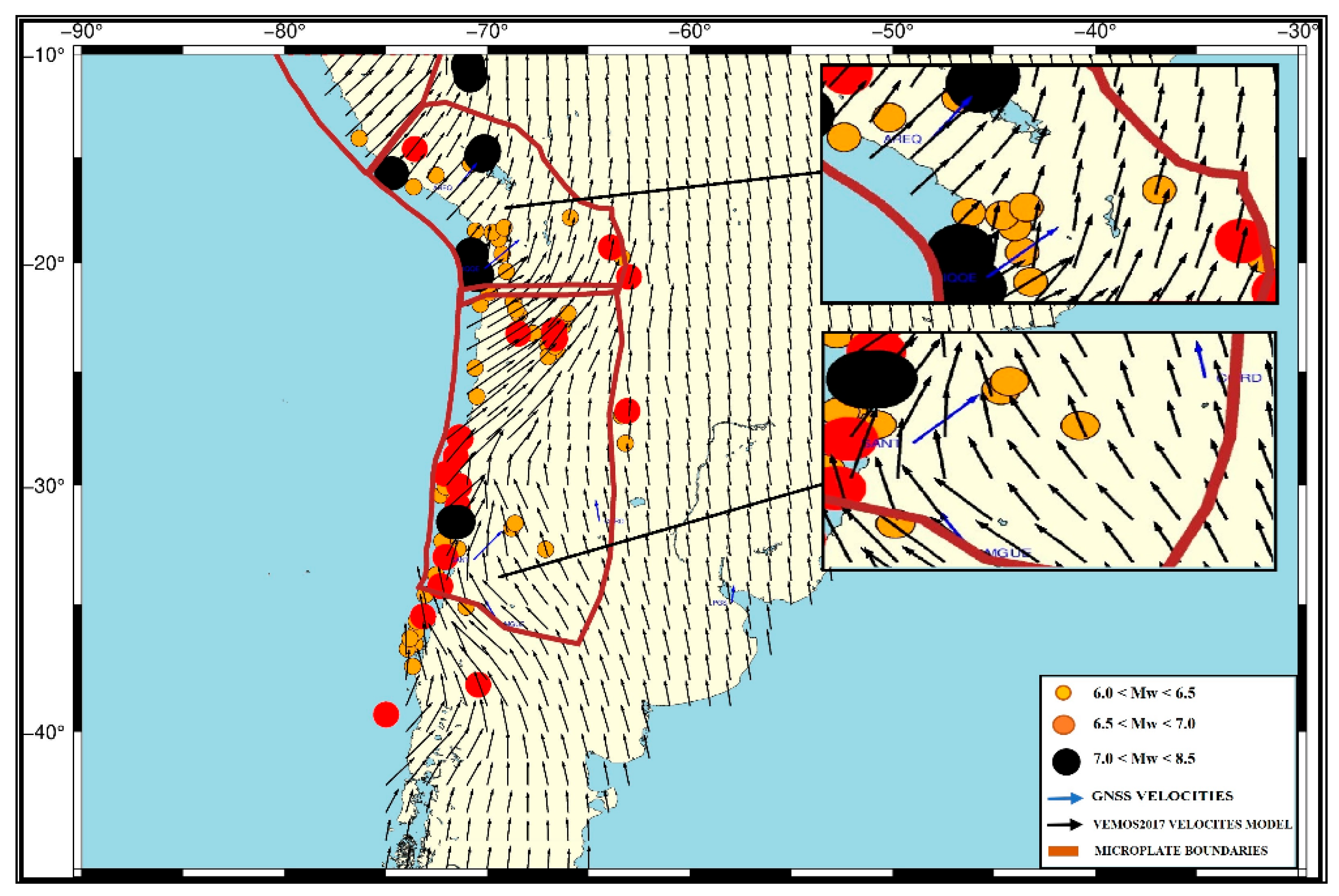
Because crustal deformation in this area is highly time-dependent, the Velocity Model for SIRGAS (VEMOS) model, which is the velocity model associated with the SIRGAS (Sistema de Referencia Geocéntrico para las Américas) reference frame, was used for comparison with our GAMIT/GLOBK results. The SIRGAS reference network, which began in 1995 with 58 stations and now comprises around 500 stations, requires frequent updates of surface deformation models, especially along the seismically active western margin of South America [35]. Comparison of our 2020–2023 solutions with the VEMOS2017 deformation model developed by Sánchez and Drewes [35] for the period 2014–2017 indicates agreement at the level of approximately 5 mm/year. The comparison of our results with VEMOS2017, in light of the earthquakes that have occurred in the region since 2015, is illustrated in Figure 8. Herman and Govers [36] examined the interaction between the South American and Nazca Plates and concluded that the Nazca Plate subducts beneath South America from southern Chile to Colombia at a rate of about 75–60 mm/year along a constant azimuth of 75–78°, generating mega-earthquakes. Along the coast, velocities of 20–30 mm/year toward the northeast are observed, decreasing to nearly 0 mm/year east of the Andes. Their study also identifies nearly trench-parallel (i.e., perpendicular to plate convergence) velocity components in northern Peru and southern Ecuador, interpreted as reflecting complex kinematics: toward the northeast in northern Ecuador and Colombia and toward the east in Chile, parallel to the direction of shortening associated with interplate locking [37]. Espurt et al. [38] investigated the flat-slab dynamics and deformation of the South American Plate and showed that the Nazca Plate is anomalously thick and buoyant and carries several topographic anomalies (aseismic ridges and oceanic plateaus). The corresponding flat-slab segments beneath South America include Peru, central Chile, northwestern Argentina and Ecuador. Stations AREQ, SANT, IQQE and MGUE are located in these zones, which explains the deviation of their observed motions from global plate models; they lie in regions where the Nazca Plate is strongly coupled to the overriding South American Plate and accumulates significant seismic strain. Jagoda [39] estimated the motion parameters of several major tectonic plates using GNSS station positions and velocities in ITRF2014, employing data from 29 GNSS stations in South America. In that study, stations along the Peru–Chile margin (AREQ, CALL, CONT, VALP, ANTC and OUI3) were excluded from the final solutions because they showed inconsistencies attributed to seismic strain accumulation due to strong coupling with the subducting Nazca Plate.

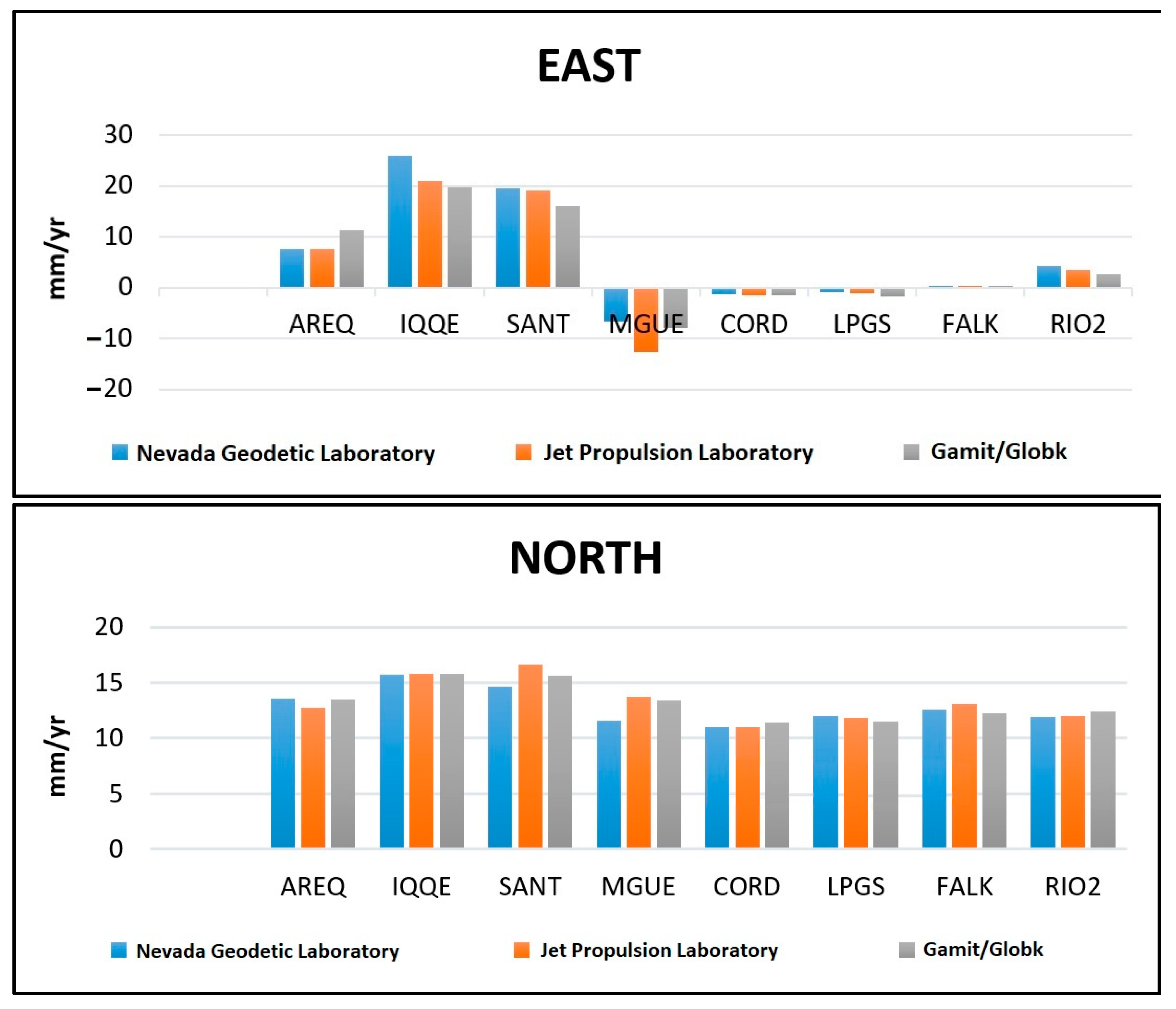
In addition, comparison of our GAMIT/GLOBK V.10.7 solutions with the velocities derived by the Nevada Geodetic Laboratory and the Jet Propulsion Laboratory for permanent stations in the region shows agreement within 1–5 mm/year in both east and north components, as illustrated in Figure 9 [40,41].

3.3. Australian Plate

The Australian Plate is one of the largest tectonic plates on Earth, encompassing the Australian continent, Tasmania, New Guinea, New Zealand, and parts of the Indian Ocean basin. As shown in Figure 1, it covers much of Southeast Asia, India, Australia and a large portion of the Pacific Ocean. The plate plays a key role in understanding global geological and tectonic processes and has been the focus of numerous studies across different disciplines. It is bounded to the east by the Pacific Plate, to the southwest by the Antarctic Plate, to the north by the Eurasian and Philippine Plates, and to the west by the African Plate. Because it shares boundaries with several other plates, a variety of tectonic processes occur along its margins. For example, the boundary between the Indian and Eurasian Plates is characterized by a strong collisional regime, while the Pacific margin is dominated by subduction zones and extensional forces. Consequently, high levels of seismicity and volcanic activity are observed along plate boundaries, particularly along the western coast of Indonesia and near the eastern margin of Australia, where numerous volcanic centers are present.

Within the plate interior, major geological structures and formations also occur. The Ninetyeast Ridge, for instance, is a prominent mid-ocean ridge feature that reflects significant intraplate tectonic activity. Such processes can produce large-scale local and regional variations in topography, contributing to uplift and basin formation. The Australian Plate also records important faulting and seismic activity during the Neogene and Quaternary periods.

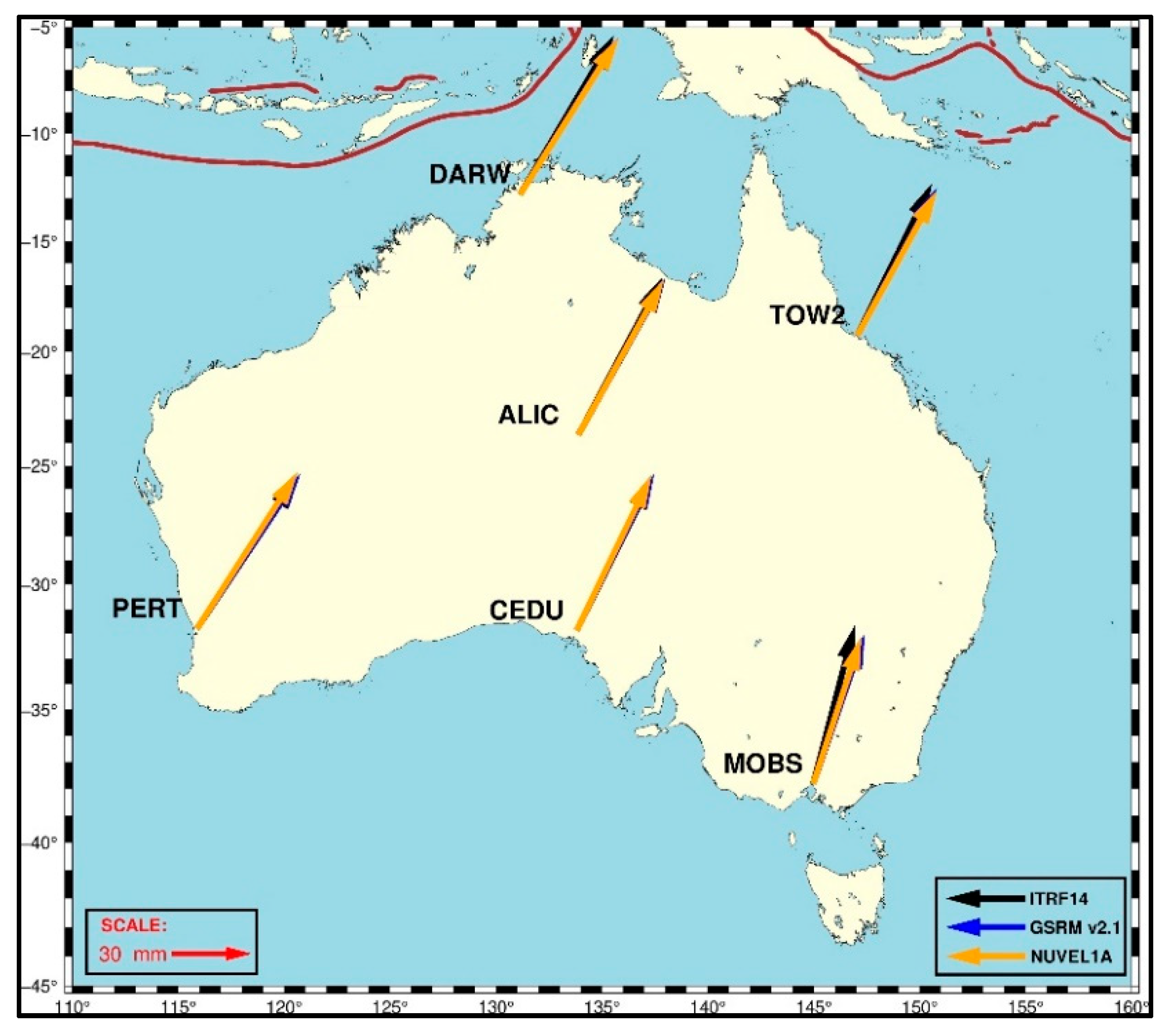
The Australian Plate has an area of about 47,000,000 km² and hosts approximately 474 permanent GNSS stations, most of which are located in the southwestern part of the continent [42]. For this study, six stations—CEDU, ALIC, TOW2, DARW, MOBS and PERT—were selected to best represent the motion of the Australian continent. Analysis of their horizontal velocities indicates that these stations move toward the northeast at rates of 60–70 mm/year. To evaluate the accuracy of these estimates, comparisons were made with the NUVEL-1A and GSRM v2.1 plate motion models (Figure 10). As shown in

Table 7. Velocities of Australian Plate GNSS stations in different plate models.

Station Name	ITRF14 Plate Model		GSRM v2.1 Plate Model		NUVEL-1A Plate Model
	N Rate (mm/year)	E Rate (mm/year)	N Rate (mm/year)	E Rate (mm/year)	N Rate (mm/year)	E Rate (mm/year)
ALIC	59.46	31.75	58.88	32.69	58.66	32.29
CEDU	58.11	28.96	58.86	29.16	58.65	28.27
DARW	59.81	35.37	59.20	36.99	59.15	37.24
MOBS	59.81	15.72	56.24	19.32	55.39	18.15
PERT	57.59	38.43	58.37	38.89	59.19	38.05
TOW2	57.24	28.13	55.57	29.99	54.60	29.91

, the differences are generally within 1–2 mm/year, indicating very good agreement. Using GNSS data from 2002–2021, Savchyn [42] determined that the Australian Plate exhibits a motion of approximately 35/71 (E/N) mm/year.

Because of its rich permanent network, coherent motion, numerous neighboring plates and high level of seismic activity, the Australian Plate has been the subject of many geodetic and geophysical investigations. Mowafy and Bilbas [43] used GNSS station data (GPS + GLONASS) in Western Australia to estimate horizontal plate motion and found a displacement of 0.0684 m/year with an azimuth of 29.65° in ITRF2008. Jagoda [39] selected 20 GNSS stations on the Australian Plate to determine plate motion parameters for all major plates based on GNSS station positions in ITRF2014. The results highlight that the Australian Plate is the most tectonically stable among the plates analyzed and, at the same time, exhibits the highest absolute plate velocity; it has been moving toward the northeast at approximately 6–7 cm/year toward the Eurasian–Pacific plates for the last 45 million years. This motion is largely attributed to the collision of India with the Asian continent. According to the corresponding research, the relatively large velocity of the Australian Plate is also closely related to the high level of seismic activity in the surrounding region [39].

The motion of the Australian Plate is primarily driven by slab pull forces associated with subduction zones in the Indonesian region. This motion is resisted by continental collision zones in the Himalaya, New Zealand and New Guinea orogens. The intraplate stress field in Australia, as inferred from focal mechanism solutions, borehole breakouts and faulting, is unusual for an intraplate region. The maximum horizontal compressive stress (sHmax) is oriented at a high angle to the north–northeastward plate motion vector. The orientation of sHmax varies regionally:

-

East–west in western and south-central Australia;

-

Northeast–southwest in northern, central and east-central Australia;

-

North–northeast–south–southwest in northeastern Australia;

-

Northwest–southeast in southeastern Australia.

These variations in stress orientation reflect the complex interaction of regional tectonic forces and the dynamic nature of plate motions affecting the Australian continent.

The Australian Plate Motion Model (APMM) is a global Earth-centered, Earth-fixed (ECEF) model aligned with ITRF2014. The currently published APMM provides the basis for the transformation used to generate Australia’s static geocentric datum (GDA2020) and the time-dependent Australian Terrestrial Reference Frame (ATRF) coordinates [44]. ITRF is realized for the Australian Plate using only about 15 stations, whereas ATRF is based on data from 109 permanent GNSS stations. APMM is a conventional Euler pole plate motion model with a 30-year validity period from 2005.0 to 2035.0. According to this model, the Australian Plate moves toward the north–northeast at a rate of approximately 7 cm/year [45].

3.4. Antarctic Plate

The Antarctic Plate shown in Figure 1 covers an area of about 60,916,000 km² and is the fifth largest tectonic plate on Earth. It comprises the entire Antarctic continent and the surrounding oceanic regions. The Antarctic Plate is bounded by the Nazca, South American, African, Somali, Australian and Pacific Plates. Its formation began roughly contemporaneously with the breakup of the Gondwana supercontinent. The separation of the Antarctic Plate toward the South Pole and the development of the Antarctic Circumpolar Current around 35 million years ago led to its isolation and glaciation.

The Antarctic continent consists of East and West Antarctica, separated by a prominent mountain range extending from northern Victoria Land around the western Ross Sea to the Weddell Sea. Almost all of East Antarctica is covered by ice 1–2 km thick, whereas West Antarctica is a relatively young province formed by the amalgamation of small microplates about 500 million years ago.

Compared with other major plates, geodynamic studies on the Antarctic Plate have advanced more slowly. The primary reasons are the large geographic extent of the plate, the harsh climatic conditions and the presence of extensive ice cover. Despite these challenges, the Antarctic Plate is of great scientific interest for geodynamic research because investigations of this region can significantly improve our understanding of the processes occurring between tectonic plates. In particular, monitoring geodynamic processes and detecting deformation on the ice-free surfaces require the development and application of GNSS techniques in conjunction with a precise and consistent terrestrial reference frame based on the most recent plate motion models.

To facilitate the observation of these geodynamic and environmental processes, permanent GNSS station networks such as the IGS and POLENET have been established across the Antarctic Plate, enabling high-precision monitoring of both horizontal and vertical crustal motions. The spatial distribution of these networks is notably heterogeneous; station density is comparatively higher in West Antarctica, where climatic and logistical conditions are relatively more favorable, whereas East Antarctica remains more sparsely instrumented due to its harsher environmental conditions and operational constraints.

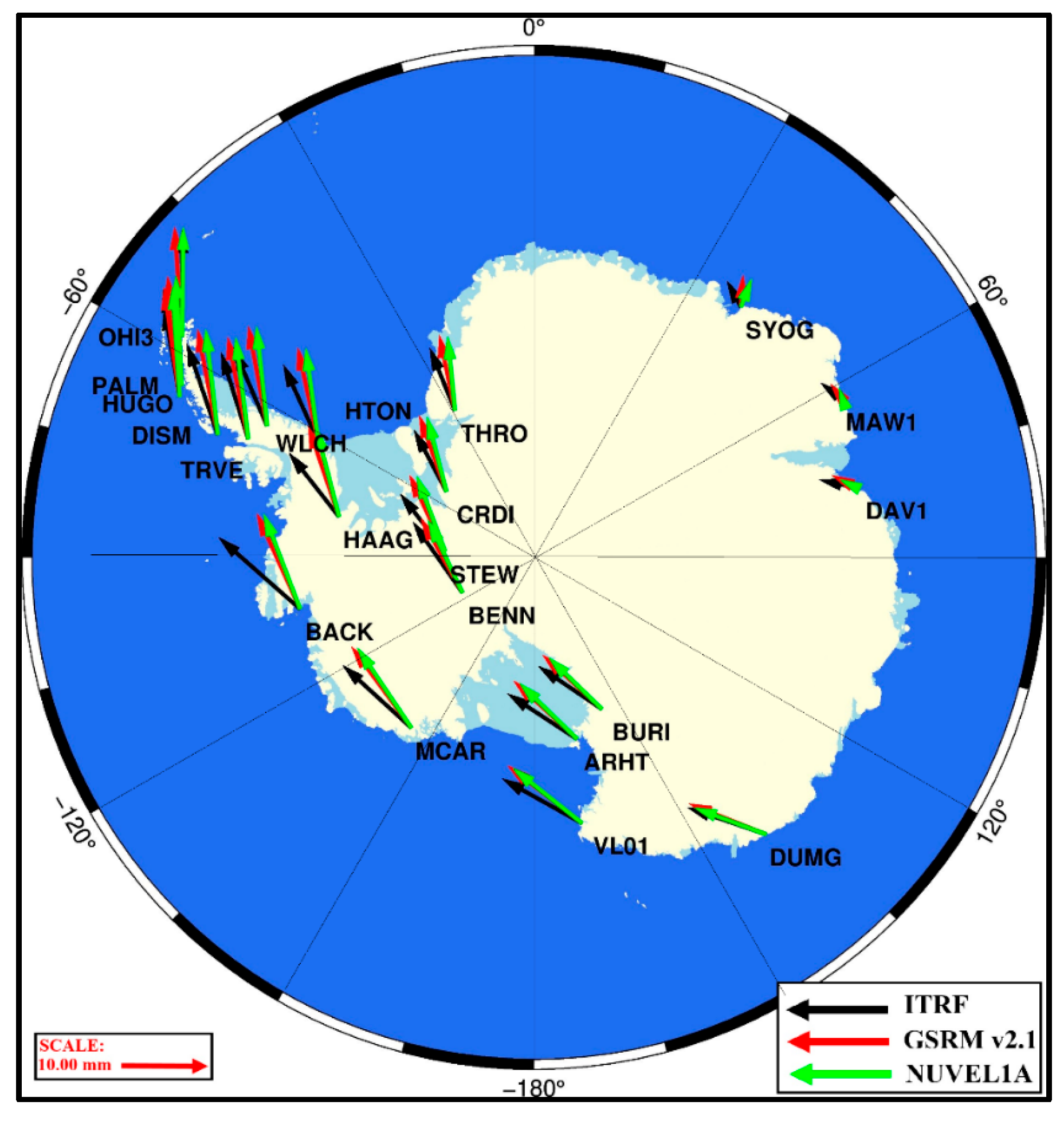
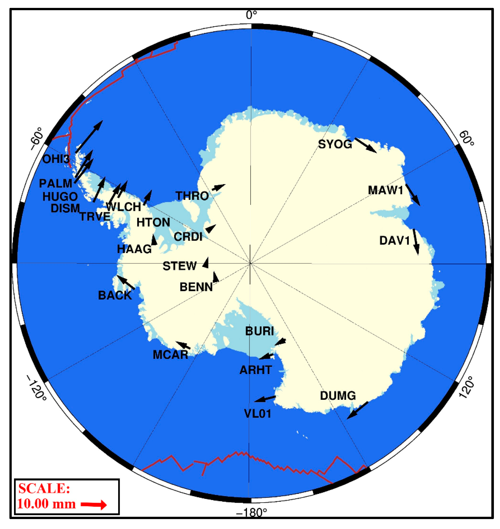
To best capture the tectonic motion of the Antarctic Plate and its interaction with neighboring plates, 22 GNSS stations were selected for analysis, 18 of which are located in West Antarctica and 4 in East Antarctica. Examination of the station velocities in the ITRF14/IGB14 reference frame shows that West and East Antarctica exhibit distinct horizontal motion patterns, as summarized in

Table 8. Velocities of Antarctic Plate GNSS stations in different plate models.

Station Name	ITRF14 Plate Model		GSRM v2.1 Plate Model		NUVEL-1A Plate Model
	N Rate (mm/year)	E Rate (mm/year)	N Rate (mm/year)	E Rate (mm/year)	N Rate (mm/year)	E Rate (mm/year)
THRO	11.72	1.32	12.92	3.86	12.00	5.00
CRDI	11.05	5.26	11.89	7.83	10.66	8.44
OHI3	10.01	15.70	11.44	15.52	10.17	16.34
HTON	11.79	8.91	11.01	12.71	9.72	13.28
WLCH	11.31	9.66	10.76	14.22	9.46	14.81
PALM	10.36	13.68	10.73	16.15	9.43	16.83
HUGO	9.02	13.13	10.52	16.36	9.22	17.01
TRVE	10.32	12.22	10.27	15.11	8.96	15.63
DISM	10.88	12.88	10.09	15.93	8.77	16.45
HAAG	10.94	9.18	8.62	14.45	7.31	14.60
STEW	8.63	9.57	7.21	12.96	5.92	12.80
BACK	11.31	15.30	3.92	17.93	2.76	17.62
BENN	2.39	14.97	0.83	14.9	−0.15	14.11
MCAR	−1.76	16.19	−5.29	16.8	−5.74	15.85
VL01	−10.08	12.38	−12.16	11.00	−11.57	10.21
ARHT	−10.46	10.00	−12.37	8.42	−11.73	7.52
BURI	−11.37	7.10	−12.85	5.59	−12.00	4.81
DUMG	−12.43	7.58	−12.74	6.92	−11.64	6.68
DAV1	−6.38	−2.88	−4.02	−3.18	−2.85	−2.19
MAW1	−2.18	−4.31	−0.68	−3.32	0.29	−2.06
SYOG	1.97	−4.78	4.48	−3.22	5.01	−1.69

. To compare our results with global plate motion estimates, the NUVEL-1A and GSRM v2.1 models were used. With the exception of stations BACK and MCAR, our ITRF14/IGB14 solutions agree with these models to within 0–5 mm/year, as shown in Table 8. The comparison of horizontal velocity vectors among NUVEL-1A, GSRM v2.1 and ITRF14 is illustrated in Figure 11, which also highlights the differing kinematic characteristics of West and East Antarctica.

In West Antarctica, particularly in the Antarctic Peninsula region, stations exhibit velocities of about 14–18 mm/year toward the northeast, whereas in East Antarctica velocities are lower, on the order of 4–6 mm/year, and generally directed toward the southwest. Overall, the horizontal displacement vectors of continuous GNSS stations indicate that the Antarctic Plate, in the ITRF14/IGB14 frame, rotates clockwise.

For BACK and MCAR, significant discrepancies are observed in the north component when comparing our results with NUVEL-1A and GSRM v2.1. As seen in Table 8, the difference in the north component is about 5 mm/year for MCAR and up to 7 mm/year for BACK. To refine the comparison, we examined the horizontal velocity components derived by the Nevada Geodetic Laboratory and the Jet Propulsion Laboratory. For BACK, the horizontal components are Vn = 9.46 mm/year and Ve = 16.63 mm/year; for MCAR, they are Vn = 2.62 mm/year and Ve = 17.18 mm/year. These values agree with our GAMIT/GLOBK V.10.7 results within 1–2 mm/year in the north component and about 1 mm/year in the east component. Furthermore, Özel et al. [46] obtained velocities of Vn = 10.39 mm/year and Ve = 15.61 mm/year for BACK and Vn = −2.86 mm/year and Ve = 16.15 mm/year for MCAR in their analysis of Antarctic plate motion, again demonstrating agreement within about 1 mm/year.

Savchyn et al. [47] used data from 60 permanent GNSS stations spanning 1994–2021 to estimate horizontal displacement vectors for the Antarctic Plate in the ITRF2014/IGS14 frame. For the stations BACK, BENN, BURI, CRDI, DUMG, HAAG, HUGO, MAW1, MCAR, STEW, SYOG and THRO, their results agree with ours to within about 1–2 mm/year. Dietrich et al. [48] analyzed data from more than 20 GNSS stations within the framework of the Scientific Committee on Antarctic Research (SCAR), using the Bernese GPS Software and expressing results in ITRF2000. Comparison of common stations shows good consistency between their horizontal velocities and those obtained in this study.

Berrocoso et al. [49] designed geodetic networks in the South Shetland Islands, Bransfield Strait and Antarctic Peninsula to investigate tectonic and volcanic processes. Analysis of GNSS campaign data collected between 1987 and 2007 indicates horizontal velocities of about 15 mm/year at stations in the Antarctic Peninsula region. Savchyn et al. [50] analyzed GNSS data from the Ukrainian Antarctic Station Akademik Vernadsky (ASAV) for the period 2019–2021 using Bernese v5.2 in the IGB08 frame and obtained a horizontal displacement vector oriented toward the northeast (Vn = 10.83 ± 0.10 mm/year, Ve = 13.43 ± 0.09 mm/year, Vu = 5.39 ± 0.29 mm/year), consistent with expected plate motion. Dietrich and Rülke [51] analyzed GNSS campaign data from SCAR campaigns conducted between 1995 and 1999 using Bernese v4.2 in ITRF2000. For common stations DAV1 (6.58 mm/year), DUMG (14.18 mm/year), MAW1 (4.49 mm/year), PALM (17.5 mm/year) and SYOG (4.35 mm/year), their horizontal velocity magnitudes agree with our GAMIT/GLOBK V.10.7 estimates to within about 1 mm/year.

3.4.1. Seismicity of the Antarctic Plate

Glacial earthquakes occur in regions hosting large ice masses such as Greenland, Antarctica and Alaska. They represent a class of seismic events first identified in long-period seismograms recorded by the Global Seismographic Network. These earthquakes are thought to be generated when large ice masses slide abruptly along their beds due to gravitational forces and their own weight, producing rapid slip along the ice–bed interface and generating earthquake-like seismic signals. Subglacial volcanic activity can also trigger motion by causing basal melting of the ice. Glacial earthquakes exhibit pronounced seasonality, occurring most frequently in late summer. Early hypotheses regarding their physical mechanism, developed from detailed analysis and interpretation of seismological data, proposed that they result from sudden slip of large ice volumes. These hypotheses have been tested using GPS measurements of ice motion, which have revealed a clear spatial and temporal relationship between glacial earthquakes and major slip events. Wiens et al. [52] combined long-period surface-wave observations with GPS measurements of ice displacement to characterize the seismogenic stick–slip behavior of the Whillans Ice Stream in West Antarctica. Their results show that the ice stream undergoes sudden slip over an area exceeding 20,000 km², with displacements of up to 70 cm [53].

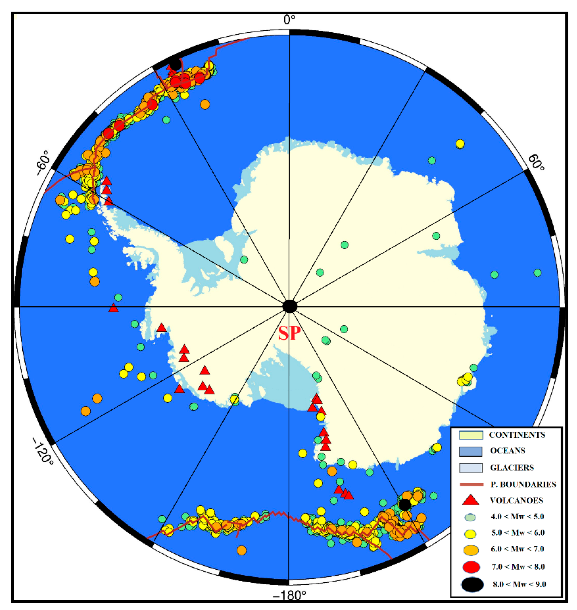
From 1990 to the present, the distribution of earthquakes and volcanic eruptions in Antarctica, shown in Figure 12, indicates that most seismic and volcanic activity occurs along the boundaries with the South American and Pacific Plates. The light green symbols on the continent mark earthquakes of moderate magnitude (Mw 4–5), many of which are interpreted as glacial earthquakes. According to the Smithsonian Institution’s Global Volcanism Program, three historical volcanic eruptions are documented in this region: Penguin Island (1905), Deception Island (1970) and Mount Erebus (1972). Volcanic and seismic activity is particularly concentrated in West Antarctica and contributes to both horizontal and vertical deformation in this area. Vries et al. [54], in their study of subglacial topography in West Antarctica, identified 138 volcanic edifices. High regional heat flow, geomagnetic anomalies and evidence of recent subglacial volcanism all suggest that the West Antarctic Rift System is currently active. In contrast, earthquakes in East Antarctica are generally intraplate events. Kaminuma [55], in his study of Antarctic seismicity, found that small earthquakes occur in West Antarctica and the Ross–Weddell graben system, but overall activity is relatively low. In the Lützow–Holm Bay (Syowa Station) region of East Antarctica, microearthquakes occur less than once per month. Along the marginal belt of the East Antarctic Shield, however, seismicity is somewhat higher. Near Victoria Land (McMurdo Station), the area around the Dry Valleys produces micro- and ultra-microearthquakes at a rate of about one event every two days. Kaminuma also concluded that West Antarctica experiences approximately 10 times more seismic activity than East Antarctica and that seismicity in volcanic regions of Antarctica is relatively higher than in surrounding areas [55].

3.4.2. Motion of the Antarctic Plate Relative to Neighboring Plates

Geological structures (plates) are evaluated in terms of both deformation and relative motion. A dynamic understanding of deformation processes requires analysis of the relative motions of the relevant plates or blocks. This approach is inherently kinematic. Relative plate motions can be considered approximately constant over geologic time intervals; accelerations and decelerations occur so slowly that the resulting forces are negligible in comparison. Constant plate velocities do not, by themselves, generate forces or deformation; rather, forces associated with relative motion arise along plate boundaries, where resistance or friction between adjacent plates is concentrated [56].

Isacks et al. proposed that seismic zones delineate the boundaries of rigid plates and that each plate is surrounded by a continuous belt of seismic activity [57]. Because seismicity reflects fault slip at high strain rates, each plate must be in relative motion with respect to its neighbors. Such relative motion can occur in three principal forms: (i) divergent boundaries, where plates move apart and new oceanic crust is created at mid-ocean ridges; (ii) convergent boundaries, where one plate subducts beneath another, leading to destructive and collisional margins; and (iii) transform boundaries, where lateral slip occurs along strike-slip faults. The location of plate boundaries determines the spatial distribution of tectonic activity, while the boundary type provides information on the nature of the tectonic processes operating there [57].

The continental part of the Antarctic Plate is characterized by very slow motion, as shown in Table 8. In East Antarctica, velocities are about 5–7 mm/year, whereas, in West Antarctica, particularly in the tectonically active northern Antarctic Peninsula, velocities exceed 15 mm/year. Along the boundaries between the Antarctic Plate and its neighboring plates, different types of motion reflecting the characteristic behavior of each boundary are observed. Table 5 lists the horizontal displacements of permanent GNSS stations on the neighboring plates, derived from GLOBK solutions in which each plate is held fixed in turn. In this section, we examine whether the horizontal motions obtained from solutions with the Antarctic Plate held fixed are consistent with the known kinematics of the corresponding plate boundaries.

Considering first the boundary between the South American and Antarctic Plates, the America–Antarctic Ridge, a 2000 km long spreading center extending from the Bouvet triple junction to the southern end of the South Sandwich Trench, accommodates slow left-lateral motion between the South American and East Antarctic Plates [58]. Barker and Lawver analyzed magnetic and bathymetric data collected over the past 50 million years east of the South Sandwich Trench to determine seafloor ages, spreading rates and directions [59]. They found that spreading rates along the South America–Antarctic Ridge vary between 18 and 30 mm/year and that spreading directions were approximately east–west, with azimuths of 120–300° around 20 million years ago. These findings indicate that the plate boundary is a left-lateral transform zone with an overall east–west orientation.

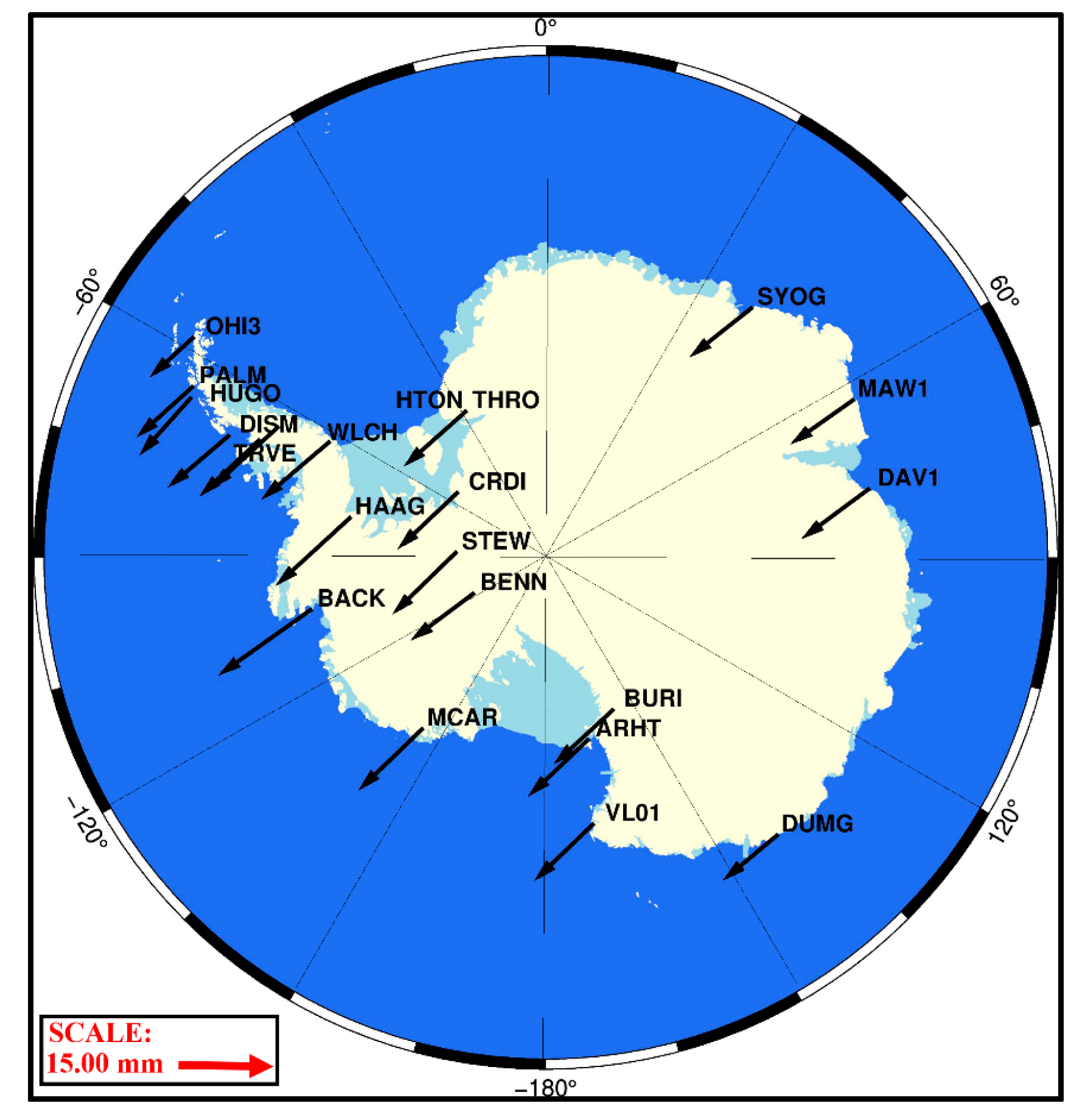
Over the last 84 million years, approximately 1320 km of left-lateral displacement in the east–west direction and 490 km of extension in the north–south direction have occurred between the southern tip of South America and the northern margin of the Antarctic Plate. Increasing separation rates and changes in plate divergence angle between about 55 and 40 Ma eventually led, around 30 Ma, to accelerated continental breakup, seafloor spreading in the western Scotia Sea and the development of the Scotia Arc [60]. According to the GLOBK solutions summarized in Table 5, with the Antarctic Plate held fixed, the horizontal velocities of stations on the South American Plate range from 6 to 29 mm/year and are oriented primarily east–west. Conversely, with the South American Plate held fixed, horizontal velocities of stations in East Antarctica are about 8–9 mm/year and those in West Antarctica are about 3–14 mm/year, directed eastward (Figure 13).

In plate-fixed solutions with the African Plate held fixed, the Antarctic Plate is observed to move away from Africa at a rate of about 14 mm/year toward the northwest (Figure 14). This divergence is associated with the formation of mid-ocean ridges between the two plates. The relative rotation pole between Africa and Antarctica has changed very little over the last 64 million years, and their relative motion has resulted in the development of the Indian–Antarctic mid-ocean ridge [61]. The paleopositions of the African, Indian and Antarctic Plates, and the origin and formation of five major aseismic structures in the western and southern Indian Ocean (the Crozet and Kerguelen plateaus, the Marion Dufresne, Lena and Ob seamount chains, and the Madagascar and Mascarene ridges), are closely related to their relative motions. Volcanic events are generally contemporaneous with major changes in relative plate motion—such as ridge jumps, asymmetric spreading and rapid changes in spreading rate or direction—that are common features of the kinematic pattern in the western and southern Indian Ocean [62]. Spreading between Africa and Antarctica occurs along the Southwest Indian Ridge between the Bouvet triple junction and the Indian Ocean triple junction [63]. In support of this, the African Plate fixed solutions in Table 5 indicate that stations HARB, SUTM and WIND in South Africa move away from Antarctica at a rate of about 11 mm/year.

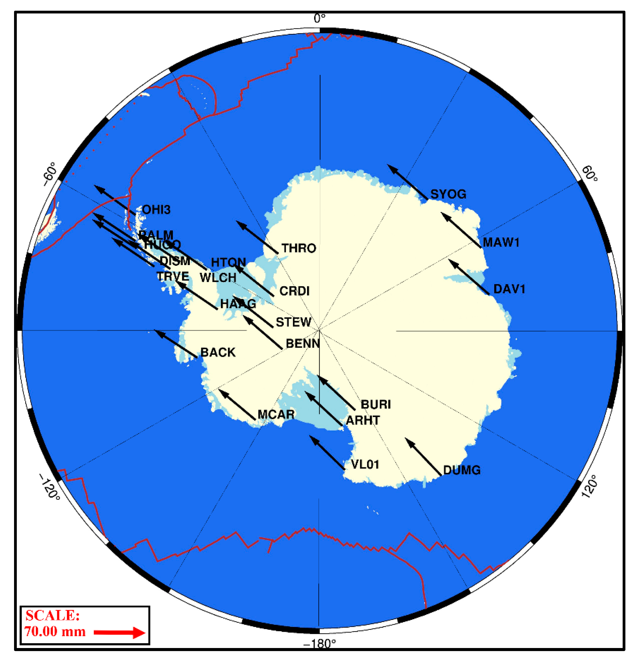
The relative motion between the Antarctic and Australian Plates also plays a key role in Southern Hemisphere plate tectonics. Along the Chile Trench, where the Antarctic Plate subducts beneath South America, relative velocities are about 20 mm/year, whereas along the Australia–Pacific Plate boundary they reach 70–100 mm/year (Figure 15). Gordon calculated angular velocities along present-day plate boundaries using the NUVEL-1 model and determined an angular velocity of 0.68° Myr⁻¹ (corresponding to ~75.6 mm/year) for the Australia–Antarctica boundary [64]. Larson et al. used data from 204 GNSS stations collected between 1991 and 1996 to estimate velocities for the African, Antarctic, Australian, Eurasian, Nazca, Pacific, North and South American Plates [65]. They compared their angular velocity estimates for the Australia–Antarctica boundary with the NUVEL-1 model and with independent solutions by Smith et al. [66] based on VLBI, SLR, GPS and DORIS observations and found angular velocities of 0.64–0.65° Myr⁻¹ (71–72 mm/year). These results indicate that the two plates are moving apart and that the plate boundary is undergoing progressive opening. The Antarctic Plate fixed solutions for stations ALIC, CEDU, DARW, MOBS, PERT and TOW2 used in this study show velocities of about 70–73 mm/year toward the northeast, consistent with these earlier estimates of Australia–Antarctica relative motion.

4. Conclusions and Recommendations

In this study, the horizontal motions of selected continuous GNSS stations located on the Antarctic, Australian, African and South American Plates were determined in the ITRF14 reference frame using the scientific software package GAMIT/GLOBK V.10.7. To compare the horizontal velocities of the stations, additional analyses were performed using different global plate motion models such as NUVEL-1A and GSRM v2.1. These comparisons show that, with the exception of stations on the western part of the South American Plate, the station velocities obtained in the ITRF14 frame are largely consistent with the predictions of the global models.

A detailed review of the literature reveals that the stations on the South American Plate exhibiting inconsistent velocities relative to the global models are located at key locations along the convergent Nazca–South America plate boundary, where one plate subducts beneath the other, and that these stations lie on microplates such as the Altiplano, Puna–Sierras Pampeanas and Peru blocks. This finding indicates that global plate models such as ITRF14, NUVEL-1A and GSRM v2.1 are insufficient for capturing the kinematics of small microplates. When the GNSS-derived station velocities are compared with the regional VEMOS2017 velocity model, which most accurately represents the kinematics of the South American Plate, the results show good agreement, further supporting this interpretation.

Examination of the time series for stations on the Antarctic Plate shows that data gaps occur in many stations, especially during the polar night. For example, the DISM station regularly exhibits interruptions in data acquisition during certain times of the year. In light of these observations, it is recommended that more robust and long-lasting power and energy storage systems (e.g., batteries, wind turbines, and similar solutions) be used to ensure continuous operation of the stations and to enable more reliable analyses and interpretations.

Analysis of the horizontal motions of Antarctic stations reveals distinct kinematic behavior between West and East Antarctica. This is most likely due to the fact that West Antarctica, particularly stations on the Antarctic Peninsula, is subject to more intense tectonic activity than East Antarctica. Seismic and volcanic activity records for the period 1990–2024 also show a concentration of events in West Antarctica.

Analysis of the results for vertical velocity components shows also significant regional differences. In East Antarctica, vertical velocities at permanent GNSS stations generally range between −1.9 and 2.4 mm/year, whereas values between −5.5 and 5.6 mm/year have been identified in West Antarctica. Moreover, extreme uplift rates reaching 17.6 mm/year (BACK) have been observed in the Amundsen Sea region. These vertical crustal motions in Antarctica represent a complex combination of the lithosphere’s response to both past and present ice mass changes. The primary factors contributing to such complex vertical movements include glacial isostatic adjustment (GIA), contemporary ice mass variations and the associated elastic response, loading effects (atmospheric and oceanic), and regional tectonic and geodynamic processes. In this context, it is clear that processes related to ice mass loss, such as glacier melting and the associated glacial earthquakes, must be considered as factors that can affect the positions and velocities of GNSS stations in the region.

By holding the South American, African and Australian Plates fixed in turn, we examined whether the horizontal motions of Antarctic stations reflect the characteristic kinematics of the corresponding plate boundaries. Previous studies indicate that the Antarctic–South America boundary is a transform-type margin, whereas the boundaries between Antarctica and Africa and between Antarctica and Australia are divergent margins, characterized by relative motions of approximately 14 mm/year and 70 mm/year in the northeast–northwest directions, respectively. Figure 16 shows that the Antarctic Plate fixed solutions obtained in this study are consistent with these boundary characteristics.

The analyses conducted in this study demonstrate that GNSS provides significant advantages over other methods for monitoring plate motion and related geodynamic processes. In particular, in regions where plate boundaries intersect and where large earthquakes occur over long time periods, GNSS observations make an indispensable contribution to the development and refinement of plate motion models. For fast-moving plates such as the Australian Plate, which moves at a rate of 70–75 mm/year, GNSS plays a crucial role in updating and maintaining the accuracy of terrestrial reference frames. Moreover, in regions where global plate models are insufficient or incomplete—especially in areas containing microplates—long-term GNSS solutions provide essential information on the motion of the plate hosting a given station and can support the development of regional plate motion models.

GNSS observations provide critical data for regional tectonic analyses and climate change models by monitoring ice sheet dynamics and continental plate motions in Antarctica with millimeter-level precision. Such high-precision measurements will enable more accurate assessments of ice loss processes, plate kinematics, and sea-level changes in future studies, particularly through the use of longer time series and broader spatial coverage. Although the three-year time series analysis applied in this study is sufficient from the plate tectonics perspective, the use of longer time series in future scientific studies will further enhance the reliability and robustness of the outcomes.

It is further anticipated that this study will contribute to the scientific research activities conducted by Türkiye in Antarctica under the leadership of TÜBİTAK (The Scientific and Technological Research Council of Türkiye), particularly in the field of plate tectonics.

References

1. Acocella, V. Corrigendum to ‘Structural control on magmatism along divergent and convergent plate boundaries: Overview, model, problems’. Earth Sci. Rev. 2014, 136, 226–288. [Google Scholar] [CrossRef]
2. USRA. Available online: https://epod.usra.edu/blog/2000/11/plate-tectonics-on-the-birthday-of-alfred-wegener.html (accessed on 9 January 2026).
3. Keller, E.A.; Pinter, N. Active Tectonics: Earthquakes, Uplift and Landscape; Prentice Hall Publishers: Upper Saddle River, NJ, USA, 1996; ISBN 10:0023632615. [Google Scholar]
4. Yavaşoğlu, H. Determination of Recent Tectonic Activity of North Anatolian Fault in Mid Anatolia Region with Geodetic Methods and Elastic Half Space Modeling. Ph.D. Thesis, Istanbul Technical University, Institute of Science and Technology, Istanbul, Turkey, 2009. (In Turkish) [Google Scholar]
5. Kahveci, M.; Yıldız, F. Theory and Application of Positioning Systems Using GPS/GNSS Satellites; Nobel Publishing: Ankara, Turkey, 2009; ISBN 9786051332659. (In Turkish) [Google Scholar]
6. Groves, P.D. Principles of GNSS, Inertial, and Multisensor Integrated Navigation Systems, 2nd ed.; Artech House: Boston, MA, USA, 2013; ISBN 978-1-58053-255-6. [Google Scholar]
7. Uzel, T.; Eren, K.; Gülal, E.; Tiryakioğlu, İ.; Dindar, A.A.; Yılmaz, H. Monitoring the tectonic plate movements in Turkey based on the national continuous GNSS network. Arab. J. Geosci. 2012, 6, 3573–3580. [Google Scholar] [CrossRef]
8. Tunini, L.; Magrin, A.; Rossi, G.; Zuliani, D. Global Navigation Satellite System (GNSS) time series and velocities about a slowly convergent margin processed on high-performance computing (HPC) clusters: Products and robustness evaluation. Earth Syst. Sci. Data 2024, 16, 1083–1106. [Google Scholar] [CrossRef]
9. Calais, E.; Bayer, R.; Chéry, J.; Cotton, F.; Doerflinger, E.; Flouzat, M.; Jouanne, F.; Kasser, M.; Laplanche, M.; Maillard, D.; et al. REGAL: Reseau GPS permanent dans les Alpes occidentales; configuration et premiers resultats. Bull. Société Géologique Fr. 2001, 172, 141–158. [Google Scholar] [CrossRef]
10. Tiryakioğlu, I. Identification of the Block Movements and Stress Zones in Southwestern Anatolia with GNSS Measurements. Ph.D. Thesis, Yıldız Technical University, Institute of Science and Technology, Istanbul, Turkey, 2012. (In Turkish) [Google Scholar]
11. Hammond, W.C.; Blewitt, G.; Kreemer, C.; Nerem, R.S. GPS Imaging of global vertical land motion for studies of sea level rise. J. Geophys. Res. Solid Earth 2021, 126, e2021JB022355. [Google Scholar] [CrossRef]
12. Hattori, A.; Aoyama, Y.; Okuna, J.; Doi, K. GNSS observations of GIA-Induced crustal deformation in Lützow-Holm Bay, East Antarctica. Geophys. Res. Lett. 2021, 48, e2021GL093479. [Google Scholar] [CrossRef]
13. Richter, A.; Popov, S.V.; Fritsche, M.; Lukin, V.V.; Matveev, A.Y.; Ekaykin, A.A.; Lipenkov, V.Y.; Fedorov, D.V.; Eberlein, L.; Schröder, L.; et al. Height changes over subglacial Lake Vostok, East Antarctica: Insights from GNSS observations. J. Geophys. Res. Earth Surf. 2014, 119, 2460–2480. [Google Scholar] [CrossRef]
14. Selbesoğlu, M.O.; Yavaşoğlu, H.H.; Karabulut, M.F.; Oktar, Ö.; Gülal, V.E.; Karaman, H.; Kamaşak, M.E. Accuracy investigation of GNSS-reflectometry for sea level monitoring on Horseshoe Island, Antarctica: Preliminary results of the Turkish permanent GNSS station (TUR1). Turk. J. Earth Sci. 2023, 32, 1013–1021. [Google Scholar] [CrossRef]
15. Pinat, E.; Defraigne, P.; Bergeot, N.; Chevalier, J.-M.; Bertrand, B. Long-Term snow height variations in Antarctica from GNSS interferometric reflectometry. Remote Sens. 2021, 13, 1164. [Google Scholar] [CrossRef]
16. Generic Mapping Tools. Available online: https://www.generic-mapping-tools.org/ (accessed on 6 December 2025).
17. USGS Earthquake Catalog. Available online: https://earthquake.usgs.gov/earthquakes/search/ (accessed on 10 January 2026).
18. NSF National Science Foundation SAGE Earthquake Catalog. Available online: https://ds.iris.edu/wilber3/find_event (accessed on 10 January 2026).
19. EarthScope Consortium. Available online: https://www.earthscope.org/data/ (accessed on 10 January 2026).
20. Herring, T.A.; King, R.W.; Floyd, M.A.; McClusky, S.C. Introduction to GAMIT/GLOBK, Release 10.7, Department of Earth, Atmospheric, and Planetary Sciences; Massachusetts Institute of Technology: Cambridge, MA, USA, 2018. [Google Scholar]
21. USGS. Available online: https://www.usgs.gov/ (accessed on 6 May 2024).
22. Estey, L.H.; Meertens, C.M. TEQC: The Multi-Purpose Toolkit for GPS/GLONASS Data. GPS Solut. 1999, 3, 42–49. [Google Scholar] [CrossRef]
23. Grewal, M.S.; Andrews, A.P. Kalman Filtering: Theory and Practice Using MATLAB, 2nd ed.; John Wiley & Sons Publications: New York, NY, USA, 2001; ISBN 0-471-39254-5. [Google Scholar]
24. Masnadi-Shirazi, H.; Masnadi-Shirazi, A.; Dastgheib, M.A. A step by step mathematical derivation and tutorial on Kalman Filters. arXiv 2019. [Google Scholar] [CrossRef]
25. Altamimi, Z.; Métivier, L.; Collilieux, X. ITRF2008 plate motion model. J. Geophys. Res. Solid Earth 2012, 117, B07402. [Google Scholar] [CrossRef]
26. Fernandes, R.M.S.; Ambrosius, B.A.C.; Noomen, R.; Bastos, L.; Combrinck, L.; Miranda, J.M.; Spakman, W. Angular velocities of Nubia and Somalia from continuous GPS data: Implications on present-day relative kinematics. Earth Planet. Sci. Lett. 2004, 222, 197–208. [Google Scholar] [CrossRef]
27. Fernandes, R.M.S.; Miranda, J.M.; Delvaux, D.; Stamps, D.S.; Saria, E. Re-evaluation of the kinematics of Victoria Block using continuous GNSS data. Geophys. J. Int. 2013, 193, 1–20. [Google Scholar] [CrossRef]
28. Gomo, S.; Durrheim, R.J.; Cooper, G.R.J. Analysis of GPS Position Time Series in Africa. In Proceedings of the South African Geophysical Association Biannual Conference, Cape Town, South Africa, 10–13 September 2017. [Google Scholar]
29. Deville, E.; Marsset, T.; Courgeon, S.; Jatiault, R.; Ponte, J.P.; Thereau, E.; Jouet, G.; Jorry, S.J.; Droz, L. Active fault system across the oceanic lithosphere of the Mozambique Channel: Implications for the Nubia–Somalia southern plate boundary. Earth Planet. Sci. Lett. 2018, 502, 210–220. [Google Scholar] [CrossRef]
30. Viltres, R.; Jónsson, S.; Alothman, A.O.; Liu, S.; Leroy, S.; Masson, F.; Doubre, C.; Reilinger, R. Present-day motion of the Arabian Plate. Tectonics 2022, 41, e2021TC007013. [Google Scholar] [CrossRef]
31. Savchyn, I. Analysis of recent African tectonic plate system kinematics based on GNSS data. Acta Geodyn. Geomater. 2023, 20, 19–28. [Google Scholar] [CrossRef]
32. Kurt, A.I. Improving Velocity Obtained from Campaign Type GPS Measurements via Utilizing Time Series Analysis of Continuous GPS Stations. Ph.D. Thesis, Istanbul Technical University, Institute of Science and Technology, Istanbul, Turkey, 2009. (In Turkish) [Google Scholar]
33. Hayes, G.P.; Moore, G.L.; Portner, D.E.; Hearne, M.; Flamme, H.; Furtney, M.; Smoczyk, G.M. Slab2, a comprehensive subduction zone geometry model. Science 2018, 362, 58–61. [Google Scholar] [CrossRef]
34. Gutscher, M.; Malavielille, J.; Lallemand, S.; Collet, J.Y. Tectonic segmentation of the North Andean margin: Impact of the Carnegie Ridge collision. Earth Planet. Sci. Lett. 1999, 168, 255–270. [Google Scholar] [CrossRef]
35. Sanchez, L.; Drewes, H. Geodetic monitoring of the variable surface deformation in Latin America. In Beyond 100: The Next Century in Geodesy, International Association of Geodesy Symposia; Freymueller, J.T., Sánchez, L., Eds.; Springer: Berlin/Heidelberg, Germany, 2020; Volume 152, pp. 197–208. [Google Scholar] [CrossRef]
36. Herman, M.W.; Govers, R. Locating fully locked asperities along the South America subduction megathrust: A new physical inter-seismic inversion approach in a Bayesian framework. Geochem. Geophys. Geosyst. 2020, 21, e2020GC009063. [Google Scholar] [CrossRef]
37. Metois, M.; Vingy, C.; Socquet, A. Interseismic coupling, megathrust earthquakes and seismic swarms along the Chilean Subduction Zone (38A degrees-18A degrees S). Pure Appl. Geophys. 2016, 173, 1431–1449. [Google Scholar] [CrossRef]
38. Espurt, N.; Funiciello, F.; Martinod, J.; Guillaume, B.; Regard, V.; Faccenna, C.; Brusset, S. Flat subduction dynamics and deformation of the South American plate: Insights from analog modeling. Tectonics 2008, 27, TC3011. [Google Scholar] [CrossRef]
39. Jagoda, M. Determination of Motion Parameters of Selected Major Tectonic Plates Based on GNSS Station Positions and Velocities in the ITRF2014. Sensors 2021, 21, 5342. [Google Scholar] [CrossRef]
40. ESA. Available online: https://www.esa.int/Applications/Satellite_navigation/Galileo/What_is_Galileo (accessed on 1 November 2024).
41. IGS. Available online: https://igs.org/about/ (accessed on 1 November 2024).
42. Savchyn, I. Determination of the recent rotation poles of the main tectonic plates on the base of GNSS data. Geodynamics 2022, 2, 17–27. [Google Scholar] [CrossRef]
43. Mowafy, A.; Bilbas, E. Quality control in using GNSS CORS network for monitoring plate tectonics: A Western Australia case study. J. Surv. Eng. 2016, 142, 05015003. [Google Scholar] [CrossRef]
44. ICSM. ATRF Technical Implementation Plan, Version 2.3. Available online: https://www.icsm.gov.au/publications/australian-terrestrial-referenceframe-technical-implementationplan-v23 (accessed on 1 November 2023).
45. McCubbine, J.; Riddell, A.; Brown, N. A Plate Motion Model of the Indo-Australian Tectonic Plate that Better Aligns with the Geodetic Coordinate System-Towards a More Precise Static Ellipsoidal Datum, ESS Open Archive 2023. Available online: https://essopenarchive.org/doi/full/10.22541/essoar.169602311.17461835 (accessed on 5 January 2024).
46. Özel, Ö.; Ural, Y.; Kellevezir, A.; Gündoğan, T.; Yalçın, F.; Peker, S.; Kılınc, H.; Demirel, İ.C.; Akpınar, İ. Turkiye’s permanent GNSS station for monitoring tectonic movements in the Antarctic continent: DISMAL (DISM) Station. Harit. Derg. 2024, 172, 17–29. (In Turkish) [Google Scholar]
47. Savchyn, I.; Brusak, I.; Tretyak, K. Analysis of recent Antarctic Plate kinematics based on GNSS Data. Geod. Geodyn. 2023, 14, 99–110. [Google Scholar] [CrossRef]
48. Dietrich, R.; Rülke, A.; Ihde, J.; Lindner, K.; Miller, H.; Niemeier, W.; Schenke, H.W.; Seeber, G. Plate kinematics and deformation status of the Antarctic Peninsula based on GPS. Glob. Planet. Change 2004, 42, 313–321. [Google Scholar] [CrossRef]
49. Berrocoso, M.; Fernández-Ros, A.; Ramírez, M.E.; Salamanca, J.M.; Torrecillas, C.; Pérez-Peña, A.; Páez, R.; Jiménez-Teja, Y.; García-García, A. Geodetic research on deception island and its environment (South Shetland Islands, Bransfield Sea and Antarctic Peninsula) during Spanish Antarctic campaigns, (1987–2007). In Geodetic and Geophysical Observations in Antarctica; Capra, A., Dietrich, R., Eds.; Springer: Berlin/Heidelberg, Germany, 2008; pp. 98–124. ISBN 978-3-540-74881-6. [Google Scholar]
50. Savchyn, I.; Otruba, Y.; Tretyak, K. The first Ukrainian permanent GNSS station in Antarctica: Processing and analysis of observation data. Ukr. Antarct. J. 2021, 2, 3–11. [Google Scholar] [CrossRef]
51. Dietrich, R.; Rülke, A. The SCAR GPS campaigns in the ITRF2000; Report 21; Scientific Committee on Antarctic Research (SCAR): Cambridge, UK, 2002. [Google Scholar]
52. Wiens, D.A.; Anandakrishnan, S.; Winberry, J.P.; King, M.A. Simultaneous teleseismic and geodetic observations of the stick–slip motion of an Antarctic ice stream. Nature 2008, 453, 770–774. [Google Scholar] [CrossRef]
53. Nettles, M.; Ekström, G. Glacial earthquakes in Greenland and Antarctica. Annu. Rev. Earth Planet. Sci. 2010, 38, 467–491. [Google Scholar] [CrossRef]
54. Vries, M.V.W.D.; Bingham, R.G.; Hein, A.S. A new volcanic province: An inventory of subglacial volcanoes in West Antarctica. Geol. Soc. Lond. Spec. Publ. 2018, 461, 231–248. [Google Scholar] [CrossRef]
55. Kaminuma, K. Seismicty in Antarctica. J. Phys. Earth 1976, 24, 381–395. [Google Scholar] [CrossRef]
56. Park, R.G. Geological Structures and Moving Plates; Springer Science+Business Media: Dordrecht, The Netherlands, 1988; ISBN 10:0412742608. [Google Scholar]
57. Isacks, B.; Oliver, J.; Sykes, L.R. Seismology and the new global tectonics. J. Geophys. Res. 1968, 73, 5855–5899. [Google Scholar] [CrossRef]
58. DeMets, C.; Merkouriev, S. High-resolution reconstructions of South America plate motion relative to Africa, Antarctica and North America: 34Ma to present. Geophys. J. Int. 2019, 217, 1821–1853. [Google Scholar] [CrossRef]
59. Barker, P.F.; Lawwer, L.A. South American-Antarctic plate motion over the past 50 Myr, and the evolution of the South American-Antarctic ridge. Geophys. J. Int. 1988, 94, 377–386. [Google Scholar] [CrossRef]
60. Cunningham, W.D.; Dalziel, I.W.D.; Lee, T.Y.; Lawver, L.A. Southernmost South America-Antarctic Peninsula relative plate motions since 84 Ma: Implications for the tectonic evolution of the Scotia Arc region. J. Geophys. Res. Solid Earth 1995, 100, 8257–8266. [Google Scholar] [CrossRef]
61. Hartnady, C.J.H.; Roex, A.P. Southern Ocean hotspot tracks and the Cenozoic absolute motion of the African, Antarctic, and South American plates. Earth Planet. Sci. Lett. 1985, 75, 245–257. [Google Scholar] [CrossRef]
62. Goslin, J.; Patriat, P. Absolute and relative plate motions and hypotheses on the origin of five aseismic ridges in the Indian Ocean. Tectonophysics 1983, 101, 221–244. [Google Scholar] [CrossRef]
63. Cande, S.C.; Patriat, P.; Dyment, J. Motion between the Indian, Antarctic and African plates in the early Cenozoic. Geophys. J. Int. 2010, 183, 127–149. [Google Scholar] [CrossRef]
64. Gordon, R.G. Present Plate Motions and Plate Boundaries. In Global Earth Physics Book: A Handbook of Physical Constants; Ahrens, T.J., Ed.; AGU Reference Shelf Series: Washington, DC, USA, 1995; Volume 1, pp. 66–87. ISBN 9780875908519. [Google Scholar]
65. Larson, K.M.; Freymueller, J.T.; Philipsen, S. Global plate velocities from the Global Positioning System. J. Geophys. Res. Solid Earth 1997, 102, 9961–9981. [Google Scholar] [CrossRef]
66. Smith, D.E.; Kolenkiewicz, R.; Dunn, P.J.; Robbins, J.W.; Torrence, M.H.; Klosko, S.M.; Williamson, R.G.; Pavlis, E.C.; Douglas, N.B.; Fricke, S.K. Tectonic motion and deformation from satellite laser ranging to LAGEOS. J. Geophys. Res. 1990, 95, 22013–22041. [Google Scholar] [CrossRef]
67. Kellevezir, A. Investigation of Velocity Information of the Antarctic Continent Using GNSS Data. Master’s Thesis, Konya Technical University, Institute of Science and Technology, Konya, Turkey, 2024. (In Turkish) [Google Scholar]
Figure 1. Current major and medium-sized plates and tectonic activity map of the world [2].
Geosciences 16 00119 g001
Figure 2. Sequence of research steps.
Geosciences 16 00119 g002
Figure 3. GNSS stations in the study area.
Geosciences 16 00119 g003
Figure 4. (a) ITRF14 horizontal position velocity components of fixed GNSS stations. (b) ITRF14 vertical position velocity components of fixed GNSS stations.
Geosciences 16 00119 g004
Figure 5. Comparison of different plate models with GAMIT/GLOBK (ITRF14 fixed) solutions (Africa).
Geosciences 16 00119 g005
Figure 6. Comparison of different plate models with GAMIT/GLOBK (ITRF14 fixed) solutions (South America).
Geosciences 16 00119 g006
Figure 7. South American plate microplates and network stations.
Geosciences 16 00119 g007
Figure 8. Comparison of VEMOS plate model and analysis results.
Geosciences 16 00119 g008
Figure 9. Comparison of GAMIT/GLOBK V.10.7 solutions with Nevada Geodetic Laboratory and Jet Propulsion Laboratory solutions.
Geosciences 16 00119 g009
Figure 10. Comparison of different plate models with GAMIT/GLOBK V.10.7 (ITRF14 fixed) solutions (Australia).
Geosciences 16 00119 g010
Figure 11. Comparison of different plate models with GAMIT/GLOBK V.10.7 (ITRF14 fixed) solutions (Antarctica).
Geosciences 16 00119 g011
Figure 12. Earthquakes and volcanic eruptions on the Antarctic plate between 1990 and 2024 [21].
Geosciences 16 00119 g012
Figure 13. South American Plate fixed solutions.
Geosciences 16 00119 g013
Figure 14. African Plate fixed solutions.
Geosciences 16 00119 g014
Figure 15. Australian Plate fixed solutions.
Geosciences 16 00119 g015
Figure 16. Antarctic Plate fixed solutions.
Geosciences 16 00119 g016