


Abstract
This study proposes a hybrid landslide displacement prediction model based on multi-strategy integrated optimization to address high nonlinearity and limited accuracy. An improved SFOA with Lévy flight, dynamic exploration adjustment, and stagnation detection enhances global search and convergence. The optimized SFOA (OSFOA) is employed to optimize CEEMDAN using minimum envelope entropy, reducing hyperparameter subjectivity and decomposing cumulative displacement into multi-scale components. The trend term is predicted by a Bayesian-optimized ARIMA, while periodic and stochastic terms are further decomposed by VMD and predicted using Bayesian-optimized SVR. GRA-MIC is applied to select key influencing factors and optimize model inputs. Results show that the proposed method improves accuracy and stability, reducing RMSE by about 82% and 52% compared with SSA-SVR and the baseline single decomposition model, respectively. The study further identifies monthly rainfall change and two-month reservoir level variation as the dominant driving factors for the displacement evolution, providing an effective and interpretable approach for complex landslide early warning.
1. Introduction
Landslides are major geological hazards involving the downslope movement of rock and soil along shear surfaces, influenced by both intrinsic geological conditions and extrinsic environmental triggers. They are characterized by sudden occurrence, high destructive potential, and frequent recurrence, posing serious threats to human life and property while hindering sustainable socio-economic development [1]. According to the 2024 National Natural Disaster Report issued by the Office of the National Commission for Disaster Prevention, Mitigation and Relief and the Ministry of Emergency Management of China, geological disasters, together with floods, affected over 53 million people, caused 709 fatalities or missing persons, and resulted in direct economic losses exceeding 263 billion CNY, ranking among the most severe disaster types.
Accurate displacement forecasting plays a crucial role in landslide monitoring and early-warning systems. While mechanical modeling provides vital mechanistic insights, it faces challenges in capturing multi-scale, nonlinear characteristics when site-specific geotechnical parameters are difficult to parameterize accurately. AI models can complement these methods by modeling complex patterns from data [2]. With advances in artificial intelligence, machine learning (ML) and deep learning (DL) models have been increasingly applied to slope displacement forecasting, showing superior ability in modeling complex nonlinear patterns [3]. To improve prediction accuracy and interpretability, time-series decomposition techniques such as Double Exponential Smoothing [4], Empirical Mode Decomposition (EMD) [5], Ensemble Empirical Mode Decomposition (EEMD) [6], and Complete Ensemble Empirical Mode Decomposition with Adaptive Noise (CEEMDAN) have been introduced to separate displacement sequences into secular, cyclical, and random components [7,8]. However, CEEMDAN remains sensitive to hyper-parameter settings, which may limit decomposition quality.
Recent studies have combined CEEMDAN with intelligent optimization algorithms such as Particle Swarm Optimization (PSO) or its variants [9,10], enhancing parameter adaptation and decomposition performance. Nevertheless, many existing optimizers suffer from limited search ability and susceptibility to local optima. Moreover, single-model prediction frameworks—whether statistical (e.g., Auto Regressive Integrated Moving Average (ARIMA) [11]), ML approaches (e.g., Support Vector Regression (SVR) [12], Random Forest (RF) [13]), or DL architectures (e.g., Long Short-Term Memory (LSTM) [14] and Bidirectional Long Short-Term Memory (BiLSTM) [15])—often lack sufficient generalization capability to capture both linear and nonlinear deformation patterns in complex landslide systems [16,17,18,19].
Recent advances in hybrid DL-based models have further expanded the methodological landscape for geohazard forecasting. Transformer-based architectures, for example, can capture long-range dependencies and spatiotemporal correlations in ground deformation data, such as in foundation pit settlement prediction [20]. Similarly, hybrid models that integrate physical models with data-driven learning have shown enhanced predictive performance. A notable example is the combination of the Newmark model with Extreme Gradient Boosting (XGBoost) for coseismic landslide susceptibility assessment [21]. In addition, hybrid frameworks that incorporate decomposition or ensemble-based strategies have been applied to ground deformation and susceptibility forecasting. Examples include the RF–Back Propagation (BP) neural network coupled model for urban ground collapse and subsidence [22], as well as physics-informed neural networks embedding slope stability mechanics into landslide prediction [23]. These developments demonstrate the growing potential of advanced DL-based hybrid models to complement traditional statistical and machine learning approaches in landslide forecasting.
In response, this study proposes a multi-strategy integrated optimization–decomposition–prediction framework for landslide displacement forecasting. An improved Starfish Optimization Algorithm (OSFOA), incorporating Lévy flight initialization, dynamic exploration probability adjustment, and stagnation detection, is applied to optimize CEEMDAN parameters. The OSFOA-optimized CEEMDAN decomposes cumulative displacement into secular, cyclical, and random components. Variational Mode Decomposition (VMD) is then applied to further refine the secular and cyclical terms. For prediction, a hybrid ARIMA–SVR model is employed, with ARIMA modeling the linear secular trend and SVR capturing nonlinear cyclical and random variations. This framework aims to improve decomposition precision, enhance prediction accuracy, and provide a reliable basis for intelligent landslide monitoring and early-warning systems.
2. Materials and Methods
To facilitate a clearer understanding of the hybrid prediction framework and the geological variables discussed in this study, the primary abbreviations and their corresponding definitions are summarized in the Abbreviations section located after the References.
2.1. Geological Setting of the Baishuihe Landslide Area
The Baishuihe landslide is located approximately 56 km upstream of the Three Gorges Dam, in Baishui River Village, Shazhenxi Town, Zigui County, Yichang City, Hubei Province, on the southern bank of the Yangtze River (110°32′09″ E, 31°01′34″ N). The slope exhibits a monoclinic bedding structure within a large valley section, with elevations ranging from 410 m at the trailing edge to the riverbank at the toe. The unstable mass measures ~600 m (N–S) by ~700 m (E–W), with an average depth of 30 m and an estimated volume of 12.60 × 10⁶ m3.
The landslide materials consist mainly of residual, alluvial, and colluvial deposits (silty soil, silty clay, gravelly soil, and pebbles), underlain by Triassic Feixianguan Formation carbonate bedrock interbedded with shale and clayey limestone. The loose structure, high permeability, and bedding slope configuration facilitate potential shear surface formation along soil–rock interfaces. Groundwater recharge is influenced by precipitation, hillslope runoff, and reservoir impoundment, while displacement is triggered by rainfall, water-level fluctuations, and seismic activity.
A monitoring network comprising 11 GPS stations and 2 reference points was established across the slope (Figure 1). Station ZG118, which records the largest and longest continuous displacements, was selected for analysis. The dataset contains 108 monthly records (January 2004–December 2012) of cumulative displacement, precipitation, and reservoir level, provided by the National Cryosphere Desert Data Center of China (http://www.ncdc.ac.cn, accessed on 3 February 2026).
Figure 1.
Location and monitoring layout of the Baishuihe landslide. (a) Map of Hubei Province and Zigui County generated using Natural Earth raster data in ArcGIS 10.8. (b) Distribution of monitoring points in the Baishuihe landslide area, obtained from the dataset “2007–2012 Changjiang Three Gorges Reservoir Area Zigu County Baishuihe Landslide Basic Features and Monitoring Data” provided by the National Cryosphere Desert Data Center (https://www.ncdc.ac.cn/portal/metadata/73b87094-20d4-4259-9668-1ee6222b84b1 (accessed on 2 March 2026)), licensed under a Creative Commons Attribution 4.0 International License (CC BY 4.0).
2.2. Analysis of Factors Influencing Landslide Displacement
The ZG118 landslide in the Zigui region is characterized by northeastward depressions and southwest highlands formed by the Huangling Anticline and Zigui Syncline. The subtropical continental monsoon climate yields an average annual rainfall of 1493.2 mm and temperatures of 17–19 °C. Precipitation is highly seasonal, concentrated from April to October, with intense rainfall events between June and September (Figure 2). Several months recorded over 150 mm, occasionally exceeding 170 mm, significantly influencing slope stability.
Figure 2.
Monitoring Data of the ZG118 Point at the Baishuihe Landslide. (a) Comparison of Baishuihe landslide cumulative displacement, rainfall and reservoir water level data. (b) Rainfall Distribution Map of the Baishuihe Landslide. (c) Comparison of cumulative displacement and rainfall of Baishuihe Landslide. (d) Comparison of cumulative displacement of Baishuihe Landslide and reservoir water level.
Historical data (Figure 2) show that in 2007, displacement increased by 792.7 mm alongside 1254 mm of rainfall, whereas lower rainfall corresponded to reduced displacement rates. These effects are linked to soil saturation, increased pore water pressure, and reduced shear strength within failure planes. However, rainfall–displacement trends are not fully synchronous, indicating contributions from groundwater fluctuations, terrain, geotechnical conditions, and human activities.
Reservoir level changes are another major driver. Since trial impoundment began in 2003, levels rose in phases to 175 m (Table 1), currently fluctuating between 145–175 m. From 2004–2007, levels were stable (135–139 m) with slow displacement (100–300 mm). A rise to ~155 m in 2010 was followed by displacement exceeding 1500 mm, and frequent > 170 m levels in 2011–2012 drove cumulative displacement beyond 2300 mm. Mechanisms include groundwater table rise, abrupt pore pressure changes after rapid level shifts, and seasonal oscillations altering slope equilibrium.
Table 1.
Table of Reservoir Filling Periods and Corresponding Water Levels for the Third Phase of the Three Gorges Reservoir.
Stage-wise deformation was observed: 2004–2006 showed low rates with seasonal variability; in 2007–2008, activity was moderate but flood-season–focused; 2009 saw a sharp surge due to rainfall and rapid drawdown; post-2010, velocity declined as conditions stabilized. Overall, precipitation and impoundment fluctuations jointly control displacement, with rapid impoundment changes and prolonged rainfall as key triggers. Based on these findings, precipitation, reservoir level, and cumulative displacement are selected as principal factors for the forecasting framework [24].
2.3. Time Series Analysis of Landslide Cumulative Displacement
Landslide displacement—the downslope movement of soil or rock under gravity—is controlled by internal geological conditions (e.g., structure, material properties) and external factors (e.g., rainfall, reservoir level changes, seismic activity).
In this study, the cumulative displacement D(t) is decomposed into three components:
- Trend T(t): Represents the long-term, irreversible deformation driven by gravity, reflecting the fundamental evolution stage controlled by intrinsic geological conditions such as the monoclinic bedding structure.
- Cyclical P(t): Represents the seasonal fluctuations induced by external hydrological triggers (rainfall and reservoir regulation), reflecting the cyclic modulation of effective stress within the slope.
- Residual R(t): Represents transient feedback to extreme environmental events or measurement noise, capturing the non-linear sensitivity of the landslide to sudden perturbations.
- The relationship is expressed as:
2.4. Multi-Strategy Integrated Optimization and Decomposition Framework
To address the limitations of the standard Starfish Optimization Algorithm (SFOA)in population diversity and adaptive search capability, a multi-strategy improved version is proposed, with key enhancements as follows [25]. The SFOA relies solely on uniform distribution for population initialization, which tends to cause population clustering in local regions and impairs the exploration capability of the solution space. To solve this problem, the Lévy flight strategy is introduced, which increases the likelihood of finding the global optimum by allowing for a more evenly distributed starting population [26]. The improved initialization formula is:
where denotes the step size scaling factor, which is set to 0.1 in the algorithm implementation; represents the Lévy flight exponent, set to 1.5 in the algorithm code, .
To regulate the balance between global exploration and local exploitation in each iteration, the initial SFOA assigns a fixed exploration probability Gp = 0.5, which fails to adapt to the current search state, leading to over-reliance on local exploitation in early phases (prone to early convergence to local optima) and the insufficient investigation of the solution space (risk of omitting optimum solutions) [27]. To address these issues, a dynamic adjustment mechanism is introduced, where Gp varies adaptively with the iteration count:
where Tmax denotes the maximum number of iterations and T represents the current iteration count.
Additionally, the Lévy flight step size scaling factor σ lacks explicit control in the initial setup, limiting performance in high-dimensional problems. Thus, a dynamic adjustment strategy is applied to σ:
where T and Tmax have the same meanings as above. This enables extensive exploration during global search and refined searches during local development, balancing exploration and exploitation.
The SFOA employs dimension-dependent exploration strategies (five-dimensional for D > 5, single-dimension for D ≤ 5), which have limitations in search capability and may lead to localized searches or trapping in local optima. To address this, the Whale Optimization Algorithm (WOA) predation behavior is integrated into the global exploration phase [28]. When the global search condition is met, the search behavior is governed by:
where ; A is the directional modification factor, C is the distance scaling factor, p determines the search strategy, and l is the disturbance component. When p < 0.5, the individual uses an exponential perturbation-based search strategy:
Enabling discontinuous exploration over the whole solution space. When p ≥ 0.5, the individual executes an encircling operation around the target solution:
Simulating the whale’s shrinking encirclement to guide convergence toward the global optimum.
To avoid the algorithm being trapped in local minima, a stagnation detection and adaptive adjustment strategy is implemented. It records the current best fitness value in each iteration: if no change is detected, the stagnation counter increments; otherwise, it resets. When the counter exceeds a threshold, Gp is adjusted to enhance global search capacity, followed by reinitializing the counter [29].
Building on OSFOA, a multi-strategy intelligent decomposition algorithm is constructed. The performance of CEEMDAN is significantly affected by parameter settings, including the number of realizations (NR), the maximum number of iterations (MaxIter), and the noise standard deviation (Nstd), improper settings may cause mode aliasing or incomplete decomposition [30,31]. Thus, OSFOA is used to calibrate these parameters with envelope entropy as the objective function. The envelope entropy of a signal x(i) is:
where a(j) is the Hilbert transform envelope of x(j), p(j) is the normalized version of a(j), and N is the total number of sample points. The optimization objective is:
VMD is used for secondary decomposition of periodic and stochastic components, solving the constrained variational problem [32]:
where and are the modal components and central frequencies, is the Dirac delta function, and ∗ denotes the convolution operator. The augmented Lagrangian is:
where is the quadratic penalty factor and is the Lagrange multiplier. Control mechanisms are introduced to prevent overfitting, including determining the number of modes via minimum envelope entropy and reconstruction error, retaining components with energy proportion > 5% or SNR > 1.5, and tracking error changes. This integrated framework effectively extracts multi-scale features, supporting accurate prediction tasks.
2.5. ARIMA-VMD-SVR Combined Prediction Framework with Correlation Analysis
The ARIMA-VMD-SVR combined prediction model integrates multiple methods to address the complexity of landslide displacement prediction. The ARIMA model, an extension of the Auto Regressive Moving Average (ARMA) model, is designed to handle non-stationary time series by converting them into stationary ones through differencing [33]. Characterized by parameters p (auto-regressive order), d (number of differencing steps), and q (moving average order), its general form is expressed as:
where Yt represents the target variable at time t, ϕi denotes the i-th order autoregressive coefficient, θj is the j-th order moving average coefficient, and εt stands for the error term at time t.
With its economical structure and reliance solely on endogenous variables, ARIMA exhibits strong forecasting accuracy for trend components, making it suitable for predicting the trend part of landslide displacement.
SVR, an extension of the Support Vector Machine (SVM) framework for regression problems, addresses nonlinear systems by mapping training samples into a high-dimensional feature space via a kernel function to construct an optimal linear regression hyperplane [34,35]. For a training sample set where yi is the output corresponding to input xi, the multivariate linear regression function in SVR is:
where W is the hyperplane’s coefficient vector, is the kernel function mapping input samples to high-dimensional space, and b is the bias term. The optimization problem minimizes model complexity and prediction error, with the solution (via Lagrangian duality) expressed as:
where are Lagrangian multipliers and is the Gaussian RBF kernel, chosen for capturing nonlinear relationships.
Correlation analysis involves Gray Relation Analysis (GRA) and Maximum Information Coefficient (MIC) [36,37]. GRA quantifies sequence correlations using:
where a and b are minimum and maximum differences from the parent sequence, and ρ stands for the resolution coefficient, which takes values between 0 and 1.
MIC measures variable relationships via mutual information:
where the marginal probability distributions are represented by p(x) and p(y), while the combined probability distribution is shown by p(x,y).
The combined use of GRA and MIC is motivated by their complementary strengths. While GRA is effective in quantifying linear sequence correlations, MIC can capture nonlinear and potentially complex dependencies between variables. This integration ensures that both linear and nonlinear relationships are accounted for during factor screening, thereby enhancing the robustness and interpretability of the selected predictors. Similar statistical treatments have been successfully applied in heterogeneous data contexts, such as disaster and transportation safety research, where rigorous factor screening improves model transparency and reliability.
In addition to point predictions, uncertainty quantification was incorporated into the framework to enhance the robustness of the forecasting results. Specifically, Gaussian-based probabilistic interval prediction was adopted to construct 95% confidence intervals for the outputs of the ARIMA and SVR models. Under the assumption that prediction residuals follow a Gaussian distribution, the mean prediction was used as the central estimate, while the variance of residuals was employed to define the upper and lower bounds of the confidence intervals. This approach provides a straightforward yet rigorous means of quantifying uncertainty, allowing the prediction framework to deliver not only deterministic displacement forecasts but also interval-based assessments of reliability.
2.6. Landslide Displacement Prediction Process
This study develops an ARIMA–VMD–SVR model for landslide displacement prediction by integrating decomposition optimization and factor screening strategies. An improved Starfish Optimization Algorithm (OSFOA) enhances the original SFOA through Lévy flight initialization, dynamic exploration adjustment, whale-based global search, and stagnation detection, improving convergence and avoiding local optima.
A sequential CEEMDAN–VMD framework separates displacement series into trend, periodic, and random components. CEEMDAN first extracts intrinsic mode functions (IMFs) while suppressing mode mixing. Its parameters—including ensemble size, noise amplitude, and maximum iterations—are optimized using OSFOA, with envelope entropy as the objective, and alternative stopping rules were evaluated to ensure robust decomposition. VMD is subsequently applied to periodic and random IMFs, with the mode count determined by simultaneously minimizing envelope entropy and reconstruction error, following statistical rigor principles shown to enhance generalization. This approach ensures stable decomposition and meaningful frequency separation suitable for prediction.
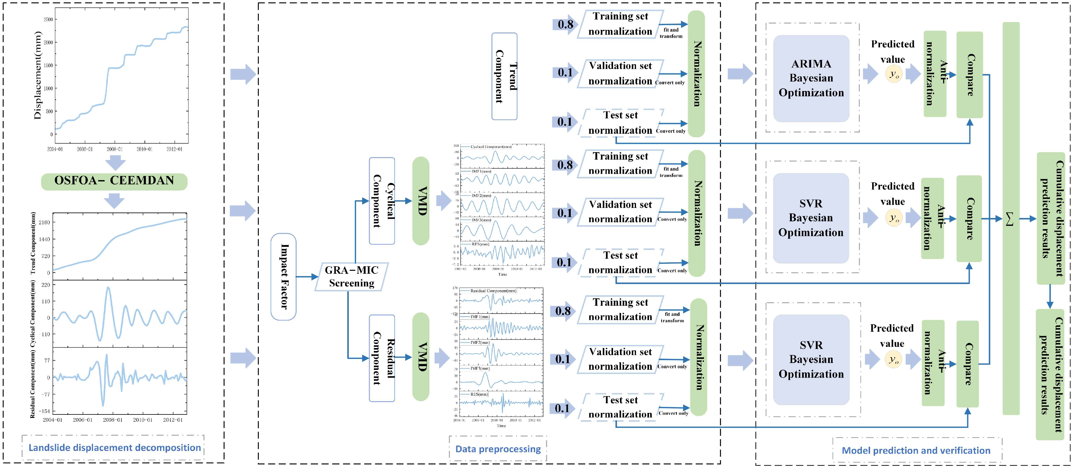
Key influencing factors for periodic and residual components are identified using GRA and MIC to enhance interpretability. The trend component is predicted by ARIMA with model order selected via Akaike Information Criterion (AIC), while subcomponents of periodic and random terms are modeled using SVR, with hyperparameters optimized through Bayesian optimization using MAE as the evaluation metric. Predictions from all components are combined to reconstruct overall displacement, and Gaussian-based probabilistic interval prediction provides 95% confidence intervals to quantify uncertainty and support early-warning applications. The implementation steps (Figure 3) are as follows:
- CEEMDAN parameter optimization: OSFOA optimizes Nstd, NR and MaxIter by minimizing envelope entropy. The optimized CEEMDAN decomposes cumulative displacement into discrete components, providing a precise basis for targeted modeling.
- Component classification: Decomposed components are categorized into trend, periodic, and random types based on their temporal characteristics. The displacement time series spans from January 2004 to December 2012, comprising a total of 108 monthly samples. Based on an 8:1:1 division ratio, 88 samples were used for model training, 10 for validation, and 10 for testing. To ensure the rigor of the validation process and prevent information leakage, the testing set was kept strictly independent and was only used for the final performance evaluation after all adaptive tuning and optimization steps were completed. The validation set was utilized solely for hyperparameter optimization and early stopping, ensuring that the reported improvements represent genuine generalization on unseen data rather than an artifact of over-parameterization on the limited dataset. This allocation ensures that each subset contains sufficient data to support reliable model development and performance evaluation. Seasonal variations in rainfall and reservoir water levels were explicitly incorporated into the modeling framework. These climatic and hydrological variables serve as the primary drivers of the periodic deformation process of landslides. The CEEMDAN–VMD effectively isolates seasonal oscillations, while rainfall- and reservoir-related indicators (e.g., monthly rainfall change and two-month reservoir level variation) capture intra-annual hydrological fluctuations. Moreover, GRA–MIC correlation analysis ensures that only the most seasonally sensitive variables are retained for modeling. Through this design, the framework captures the coupling effects between seasonal climatic cycles and slope deformation, enhancing both physical interpretability and generalization capability. All experiments were conducted using MATLAB 2023b on a Windows 10 Professional (64-bit) system. Random seed values were set to 3 to ensure reproducibility. Computations were performed on a workstation with an Intel Core i7-9700 CPU (Intel Corporation, Santa Clara, CA, USA), 32 GB Kingston DDR4 2666 MHz RAM (Kingston Technology Corporation, Fountain Valley, CA, USA), and an NVIDIA Quadro P620 GPU (NVIDIA Corporation, Santa Clara, CA, USA). Model training and validation procedures, including data preprocessing, decomposition, and sub-model updates, were carried out consistently across all experiments.
- The ARIMA model forecasts the trend component, where the AIC is employed as the evaluation function to select the optimal model order. This ensures that the chosen ARIMA specification balances model fit with complexity, thereby providing a parsimonious yet accurate representation of long-term displacement trends.
- Factor screening: Nine candidate influencing factors for periodic and random components are assessed using dual correlation analysis—GRA for similarity measurement and MIC for nonlinear association detection. Only factors meeting both criteria are retained to reduce complexity and enhance interpretability.
- Secondary decomposition and SVR modeling: VMD is applied to periodic and residual components to extract subcomponents. Each subcomponent is predicted via SVR, with factors retained as auxiliary inputs. The hyperparameters of SVR are tuned through Bayesian optimization, using mean absolute error (MAE) as the evaluation function to minimize prediction bias and enhance robustness. Predictions from subcomponents are summed to reconstruct the periodic and random components. A control experiment without VMD is conducted for performance comparison.
- Model evaluation: Final displacement predictions combine ARIMA trend forecasts with SVR-based periodic and random results. To ensure fairness across models, different evaluation functions were adopted in line with model characteristics: AIC for ARIMA order selection, and MAE for SVR hyperparameter tuning. Model performance is compared against five benchmark models using RMSE, MAE, MAPE, MSLE and R2, demonstrating the proposed framework’s accuracy and robustness.
- Finally, the predicted displacement series are presented together with their 95% confidence intervals, thereby providing both central forecasts and uncertainty ranges to support more reliable landslide early-warning applications.
Figure 3.
Overall procedure of landslide displacement prediction.
3. Result
3.1. OSFOA Performance Test
The performance of the suggested OSFOA optimization technique is verified using eight international standard test functions, as shown in Table 2 and Figure 4. The test functions F1–F4 are unimodal, whereas the test functions F5–F8 are multimodal. The algorithm’s local search capacity and convergence speed are evaluated using the unimodal functions, while its global search proficiency is evaluated using the multimodal functions.
Table 2.
Benchmarking functions.
Figure 4.
Test function 3D graph.
Comparative tests with several advanced metaheuristic algorithms—Gray Wolf Optimizer (GWO), PSO, Sparrow Search Algorithm (SSA), and OSFOA—are used in this work to verify the effectiveness of the suggested approach. Since optimization methods are stochastic, all algorithms use a uniform population size of 30 and a maximum iteration count of 300 to guarantee data dependability and result comparability. The mean and standard deviation of thirty separate trials are statistically analyzed to thoroughly assess each algorithm’s optimization potential and stability (Table 3). Figure 5 shows the iteration processes of the method and tabulates the experimental data.
Table 3.
Comparison of test results of optimization algorithm benchmark functions.
Figure 5.
Optimization algorithm comparison and iteration effect diagram.
OSFOA shows the capacity to optimize and converge quickly in unimodal benchmark functions. In contrast to the traditional SFOA and other metaheuristic algorithms already in use, OSFOA dynamically controls the exploration probability GP, bringing it closer to the global optimum in the early iterations. The addition of a more effective global search method also significantly quickens the algorithm’s pace of convergence. Combining a stagnation detection and adaptive adjustment strategy with a Lévy flight-based population initialization mechanism to boost solution diversity, OSFOA successfully improves the convergence efficiency and optimization precision for multimodal benchmark problems. Early in the search process, for example, the majority of comparison algorithms become stuck in local optima when using the F6 multimodal benchmark. By using stochastic Lévy step sizes, OSFOA effectively prevents premature convergence. This is achieved by coordinating global search and stagnation detection procedures, as well as by utilizing adaptive exploration probability management. It takes less than 50 iterations to reach the global optimum in the end. These results demonstrate that integrating many strategic modifications significantly boosts optimization performance compared to the SFOA. Moreover, when considered in the broader methodological context, OSFOA shows faster convergence and greater stability than other metaheuristics such as PSO, GA, and DE, which have also been successfully adapted for modeling tasks.
3.2. Decomposition of Landslide Cumulative Displacement Using OSFOA-CEEMDAN
The OSFOA is integrated into the CEEMDAN framework to optimize its three main parameters: Nstd, NR, and MaxIter. This yields a more refined decomposition of displacement signals and improves the predictive accuracy and generalization ability of the landslide displacement forecasting model. With the OSFOA-CEEMDAN technique, the number of optimization iterations is set to 20 and the population size is set to 30. Nstd within [0.1, 0.5], NR within [10, 100], and MaxIter within [100, 1000] are the parameters’ search ranges.
After multiple iterations, the optimal result is Nstd = 0.1, NR = 100, MaxIter = 261. A minimal envelope entropy value of 4.3105 is reached using the fitness function. The cumulative landslide displacement is then broken down using the CEEMDAN algorithm with the matching optimum parameter set. Figure 6 shows the breakdown results that were obtained.
Figure 6.
Decomposition of cumulative displacement of Baishuihe landslide ZG118.
After the decomposition, three components of the IMF are produced. Of them, IMF1 shows a clear trend, IMF2 clearly demonstrates periodic features, and IMF3 shows large swings with irregular changes, which are mostly caused by random disturbances in the landslide displacement process. Accordingly, IMF1 is the trend component, IMF2 is the cyclical component (since it is more periodic than IMF3), and IMF3 is the residual component.
3.3. Prediction of Landslide Displacement Components
3.3.1. Prediction of Trend Component of Displacement
The trend component provides crucial information about the overall movement patterns and acceleration or deceleration tendencies, primarily reflecting the long-term fluctuations in landslide displacement over time. After decomposition with the CEEMDAN method, this component becomes substantially smoother, allowing long-term displacement trends to be represented more clearly. To further enhance prediction accuracy, the ARIMA model is applied to forecast the trend component. Its hyper-parameters are optimized using Bayesian optimization, where the search ranges are set as p from 0 to 5, d from 0 to 2, and q from 0 to 5. The optimal configuration, determined according to the minimum AIC, is found to be p = 4, d = 1, and q = 0. For consistency across all component models, the trend sequence is divided into training, validation, and test sets using an 8:1:1 ratio, in line with the approach applied to the periodic and residual components. Based on this parameter setting, a univariate prediction approach is adopted, yielding excellent agreement with the observed values, as evidenced by an R2 of 0.998, an RMSE of 0.087 mm, and an MAE of 0.062 mm, with the 95% confidence interval of the predictions also illustrated in Figure 7. It can be observed that the predicted curve aligns closely with the measured data. To address the visual overlap caused by high fitting accuracy, the absolute error (residual) plot is provided at the bottom of Figure 7. These residuals remain extremely low (within ±0.2 mm) during the testing period, which confirms that the OSFOA-optimized ARIMA model effectively captures the long-term monotonic evolution with high fidelity.
Figure 7.
Comparison of Predicted and Actual Values for the Trend Component of Displacement.
3.3.2. Prediction of the Cyclical Component of Displacement
The cyclical deformation process of landslides caused by seasonal climatic change is represented by the periodic term. Rainfall and reservoir water levels are two hydrological variables that have a direct impact on this deformation process. In light of their hysteresis, nonlinear response, and interrelationships, this study methodically builds possible influencing elements based on rainfall, reservoir water levels, and landslide displacement.
Given that the response of landslide deformation to hydrological factors such as rainfall infiltration and reservoir water level fluctuations usually exhibits obvious hysteresis and nonlinear behavior, such as geological mechanisms such as hysteretic changes in pore pressure, groundwater conduction paths, and soil plastic deformation, this paper constructs influencing factors with time lag characteristics: the rainfall category includes the rainfall of the previous month (R1), the monthly rainfall change (R2), and the two-month rainfall change (R3); the reservoir water level category includes the average reservoir water level of the previous month (W1), the monthly reservoir water level change (W2), and the two-month reservoir water level change (W3); the landslide displacement category selects the landslide displacement of the previous month (D1), the monthly landslide displacement change (D2), and the two-month landslide displacement change (D3).
In order to further characterize the coupling relationship between multiple factors in cyclical landslide deformation, this paper further constructed several representative interaction terms and nonlinear terms based on the screening of high-correlation single variables. In terms of interaction terms, R1·W1 represents the coordinated changes in rainfall and reservoir water levels in the previous month, R1·D1 and W1·D1 reflect the modulation effect of hydrological disturbances on historical displacements, and D1·R2 and D2·R2 reveal the linkage trend between landslide deformation rate and rainfall changes. In terms of nonlinear terms, R12, W12, and D12 are used to characterize potential threshold effects and nonlinear response characteristics of landslides to hydrological factors, thereby supplementing the system complexity that is difficult to capture with linear variables. Subsequently, the GRA and MIC methods were used to comprehensively evaluate the correlation between each influencing factor sequence and the periodic term. When the GRA correlation degree and MIC of an influencing factor were greater than 0.7 and 0.35, respectively, it was deemed to have a high connection with the cyclical component. Figure 8 and Figure 9 show the correlation evaluation findings.
Figure 8.
GRA-MIC Correlation Analysis of Univariate Factors for the Cyclical Component.
Figure 9.
GRA-MIC Correlation Analysis of Interaction and Nonlinear Factors for the Cyclical Component.
As shown in the figures above, this paper analyzes the correlation between influencing factors and periodic term shifts at both the univariate and composite variable levels. Figure 8 shows the GRA-MIC correlation analysis results for each univariate and the periodic term. The results indicate that R2, W3, D1, D2, and D3 meet the correlation screening criteria. Furthermore, Figure 9 introduces composite variables to explore potential nonlinear relationships and interaction effects.
When there are many monthly influencing factors of the same type (for example, D2 and D3 both represent monthly landslide displacement data), the prediction model needs to map multiple variables into a high-dimensional space, which can reduce the model’s computational efficiency and have limited impact on improving prediction performance. Therefore, this paper retains only the most highly correlated influencing factors of the same type as an input variable, ultimately selecting R2, W3, D1, and D3 as the input factors for the periodic term prediction model.
A physical mechanism analysis of the above screening results shows that their selection has sufficient geotechnical rationality. The monthly rainfall change R2 reflects the direct impact of rainfall intensity on slope seepage and pore water pressure, and is the key dynamic load that induces cyclical deformation. Specifically, intensive rainfall increases the bulk unit weight of the sliding mass and generates hydrodynamic pressure, which reduces the effective normal stress on the potential failure surface. The reservoir water level change W3 between two months characterizes the regulatory effect of reservoir water level fluctuations on the slope foot back pressure and groundwater level. The ‘step-like’ displacement acceleration observed in the monitoring data (Figure 2) often coincides with periods where rapid reservoir drawdown occurs simultaneously with peak rainfall. During these periods, the outward hydraulic gradient increases significantly, creating a destabilizing seepage force that drives the cyclical evolution. The selection of D1 and D3 reflects the ‘memory effect’ or inertia in the landslide deformation process. Therefore, this combination of influencing factors is not only highly correlated statistically, but also can reasonably explain the driving force of the cyclical deformation in terms of physical mechanism.
Furthermore, although the composite variable W1·D1 exhibits a strong correlation in the GRA-MIC analysis, its introduction into the SVR model actually leads to a decrease in the prediction accuracy of the period term, indicating that its perturbation to the model outweighs its benefits. Therefore, this paper does not include this interaction term in the final modeling variables.
On the other hand, given that the periodic term sequence after CEEMDAN decomposition may still suffer from modal aliasing and overlap of high- and low-frequency components, which in turn affects the prediction model fitting effect, this paper further implements VMD secondary decomposition of the periodic term. By decomposing and extracting detailed features and multi-scale information from the periodic term, the modal aliasing problem is effectively alleviated, data features are fully extracted, and the quality of model input data is improved.
The cyclical component is predicted in this study using the SVR model. First, the original cyclical component is decomposed into several sub-components using the VMD algorithm, as shown in Figure 10. During the decomposition process, this paper determined the modal number to be 4 based on the dual criteria of minimum envelope entropy and minimum reconstruction error. After verification, the energy proportion of the four decomposed components (IMF1-3 and RES) all exceeded 5%, which was considered to contain significant periodic signal characteristics. Therefore, all of them were retained for subsequent modeling. Subsequently, the hyper-parameters of the SVR models corresponding to each sub-component are optimized using Bayesian optimization, with MAE employed as the evaluation function to guide the search toward minimizing prediction bias and improving robustness. The search ranges are specified as follows: BoxConstraint [0.01, 30], KernelScale [0.01, 5], and Epsilon [0.01, 1]. The optimized hyper-parameter configurations are listed in Table 4, with the RBF selected uniformly as the kernel. For consistency with the trend and residual components, each sub-component sequence is divided into training, validation, and test sets using an 8:1:1 ratio. The overall prediction was derived by combining the expected values of all the sub-components after hyper-parameter optimization, which involved modeling and forecasting each sub-component separately. In terms of prediction accuracy, the SVR model improved with secondary VMD performs noticeably better than the baseline SVR model, as shown in Figure 11, with an approximate 50.86% reduction in RMSE. With an RMSE of 1.47 mm, a MAE of 1.07 mm, and a R2 value of 0.998, the final prediction results for the cyclical component show good model performance, with the 95% confidence interval illustrated in Figure 11 further confirming the robustness of the forecasts.
Figure 10.
Components Obtained from the VMD Secondary Decomposition of the Cyclical Component.
Table 4.
SVR Hyper-parameters Corresponding to Each Subcomponent of the Cyclical Component.
Figure 11.
Comparison between predicted and observed values of the cyclical component displacement.
3.3.3. Prediction of the Residual Component of Displacement
This study considers the random term (residual) after CEEMDAN decomposition as a mixed signal rather than pure random noise. We believe that this term contains both true random components, such as measurement errors, and high-frequency deterministic information driven by factors such as sudden heavy rainfall and rapid changes in reservoir water levels, which is not fully captured by the previous model. Therefore, this study uses the SVR model to predict this term. Its core goal is to maximize the separation and fitting of these residual deterministic patterns, rather than predicting the purely random components, thereby supporting the improvement of the overall model’s final prediction accuracy.
This study continues the process of screening periodic predictors, employing a combined GRA and MIC assessment method to select a sequence of influencing factors highly correlated with the prediction target. Precipitation factors include the previous month’s rainfall (R1), the monthly rainfall change (R2), and the two-month rainfall change (R3). Reservoir water level factors include the previous month’s average reservoir water level (W1), the monthly average reservoir water level change (W2), and the two-month average reservoir water level change (W3). Landslide displacement factors include the previous month’s landslide displacement (D1), the monthly landslide displacement change (D2), and the two-month landslide displacement change (D3).
On this basis, considering the interaction relationship between different categories of variables, in order to further explore the hidden nonlinear coupling characteristics, 9 groups of interaction terms and nonlinear terms were constructed, including R1·D1, R1·W1, R1·D2, W1·D1, W1·D2, W1·R2, D2·R2, W2·D1, and W2·R3.
The GRA and MIC values between each affecting factor and the target prediction sequence were then calculated. An influencing factor was considered to be strongly associated with the prediction target if its MIC was larger than 0.3 and its GRA correlation coefficient was greater than 0.7. The associated outcomes are depicted in Figure 12 and Figure 13.
Figure 12.
GRA-MIC Correlation Analysis of Univariate Factors for the Residual Component.
Figure 13.
GRA-MIC Correlation Analysis of Interaction and Nonlinear Factors for the Residual Component.
As can be seen in the figure, the three selected influencing factors all exhibit varying degrees of correlation with the random term displacement data. After screening, the influencing factors that ultimately meet the set criteria include: R3, W3, D1, and D3. Because no monthly influencing factors of the same type exist, all four of these factors are used as input variables for the random term prediction model.
Similarly, analysis of the screening results for the random influencing factors reveals that their selection has a reasonable physical explanation. Random terms primarily capture disturbances caused by sudden or nonlinear factors. The two-month rainfall change R3 and the two-month reservoir water level change W3 may reflect certain hysteresis or cumulative effects. When these effects exceed a critical threshold, they trigger unpredictable sudden displacements. The introduction of the previous month’s landslide displacement D1 and the two-month landslide displacement change D3 demonstrates that even random perturbations have a probability and magnitude related to the recent level of landslide activity. An already active landslide body may be more sensitive to minor perturbations, thus exhibiting greater randomness. Therefore, this set of influencing factors aims to capture the nonlinear threshold effects and state dependence that drive the random components of landslide displacement from a physical perspective.
Furthermore, although the composite variables R1·D1 and W1·D1 also meet the GRA-MIC screening criteria and exhibit certain interactive correlations, actual prediction experiments show that incorporating them into the model actually increases model complexity and reduces training efficiency. Furthermore, prediction accuracy on the test set does not significantly improve, and even slightly decreases. Therefore, this paper ultimately does not include these interactive variables in the random term prediction model to ensure a balance between accuracy and complexity.
Similar to the prediction of periodic term displacement, the SVR prediction model is used to predict the random term. First, the original residual component is subjected to secondary decomposition using VMD; Figure 14 shows the outcomes. Similarly, based on the aforementioned control mechanism, the modal number was determined to be 4, and the four decomposed components all passed the signal-to-noise ratio (SNR) test and were considered to contain effective high-frequency information caused by sudden factors. Therefore, all of them were included in the subsequent SVR prediction model. After that, a separate SVR model is created for every deconstructed subcomponent, and the hyper-parameters are adjusted using Bayesian optimization, with MAE employed as the evaluation function to guide the search toward minimizing prediction bias and improving robustness. The search ranges are specified as follows: BoxConstraint [0.01, 30], KernelScale [0.01, 5], and Epsilon [0.01, 1].
Figure 14.
Components from the VMD Secondary Decomposition of the Residual Component.
Table 5 summarizes the optimum hyper-parameter values for all models using the RBF kernel. For consistency across all component models, each subcomponent sequence is divided into training, validation, and test sets using an 8:1:1 ratio. To create the final residual component prediction, each subcomponent is modeled and forecasted, and then its expected outputs are combined. With an approximate 84.63% reduction in RMSE, the SVR model improved by secondary VMD significantly beats the baseline SVR, as shown in Figure 15. The final prediction metrics for the residual component are 2.49 mm for the RMSE, 2.11 mm for the MAE, and 0.939 for the R2, with the 95% confidence interval shown in Figure 15 providing additional evidence for the reliability of the forecasts.
Table 5.
SVR Hyper-parameters Corresponding to Each Subcomponent of the Residual Component.
Figure 15.
Comparison between Predicted and Actual Displacement Values of the Residual Component.
3.3.4. Validation of Cumulative Displacement Prediction
As described in the preceding sections, the cumulative predicted displacement of the landslide can be obtained by summing the predicted results of the trend component, cyclical component, and residual component. The integrated prediction results are presented in Figure 16. Although the predicted and actual curves overlap significantly due to the high model precision (R2 = 0.996), the absolute error bars provided at the bottom of Figure 16 explicitly quantify the residuals during the testing months. The results indicate that the proposed model achieves high prediction accuracy, with an RMSE of 3.31 mm and an MAE of 2.95 mm, while the 95% confidence interval illustrates that the predicted cumulative displacement closely envelopes the observed values. These minimal deviations, reported on an independent 10-month testing set, demonstrate that the visual overlap is a result of genuine out-of-sample forecasting accuracy rather than in-sample fitting. Experimental analysis further demonstrates that the OSFOA-CEEMDAN-ARIMA-VMD-SVR hybrid prediction model can effectively capture the future variation trend of cumulative landslide displacement, offering both reliable prediction performance and valuable application potential.
Figure 16.
Predicted and Observed Cumulative Landslide Displacement.
3.3.5. Validation of Model Prediction Performance
To comprehensively and objectively evaluate the performance of the proposed model, we conducted comparative experiments using various landslide displacement prediction models. The following three groups of five comparison models were used for this experiment. To ensure a fair comparison, all models were trained and tested on the same Baishuihe landslide ZG118 monitoring dataset, and their key hyperparameters were optimized using a unified Bayesian optimization strategy.
To validate the value of this study’s “decomposition-prediction-ensemble” framework, we constructed two end-to-end models: SSA-SVR and SSA-BiLSTM-Attention. The former represents an optimized traditional machine learning method, while the latter represents a deep learning method incorporating an attention mechanism. To highlight the advantages of our “quadratic decomposition” strategy, we selected two single-decomposition models, CLSSA-VMD-SVR and CLF-SSA-VMD-BiLSTM-Attention, which have performed well in related research. We replicated these two models on the dataset used in this study to ensure a consistent baseline for comparison. To verify the rationality of our proposed “CEEMDAN-first, VMD-later” decomposition order, we constructed the OSFOA-VMD-ARIMA-CEEMDAN-SVR model. The only difference between this model and our model is that it uses VMD as the initial decomposition method.
All comparative experiments were comprehensively evaluated using three standard metrics: RMSE, MAE, MAPE, MSLE and R2. The results are shown in Figure 17 and Table 6. To further account for model uncertainty, 95% confidence intervals were calculated for all comparative models, and these are illustrated in Figure 17, allowing the robustness of the results to be visually assessed.
Figure 17.
Comparison of Cumulative Landslide Displacement Predictions Using Different Models.
Table 6.
Comparison of Predicted Landslide Displacement Results Using Different Models.
The data in the table indicate that the proposed OSFOA–CEEMDAN–ARIMA–VMD–SVR model demonstrates superior predictive performance across all evaluation metrics. In this case study, compared to baseline models without decomposition (such as SSA-SVR), the proposed model achieved approximately an 82% reduction in RMSE, with corresponding improvements in MAE, MAPE, and MSLE, and an approximately 12% increase in R2, highlighting the effectiveness of the signal decomposition strategy in capturing complex landslide displacement patterns. It should be noted that for cumulative displacement series reaching several thousand millimeters, the large denominator in the MAPE calculation naturally leads to artificially low percentage values (e.g., ~0.1%). While MAPE is reported for comparison, it becomes less informative for such large-magnitude series. Therefore, in this study, we prioritize absolute indicators, specifically RMSE and MAE, as the primary metrics for evaluating prediction residuals to ensure a rigorous and transparent assessment of the model’s performance. Even when considering the 95% confidence intervals, the proposed model consistently outperformed the baseline, further confirming the statistical robustness of these improvements. Compared with advanced single-decomposition models (such as CLF-SSA-BiLSTM-Attention), the proposed model achieved significant reductions in RMSE, MAE, MAPE, and MSLE, with RMSE reduced by approximately 52%, indicating that the secondary decomposition strategy can further exploit intricate patterns in the data and enhance prediction accuracy.
Furthermore, comparisons with ablation experimental models show that the “CEEMDAN-first, VMD-second” order employed in this paper outperforms the “VMD-first, CEEMDAN” order. This may be because CEEMDAN can more effectively separate the macroscopic trend, periodic, and random terms with clear physical meaning from the raw accumulated displacements, providing a purer input signal for the subsequent VMD refine. In summary, the combined prediction framework proposed in this study is effective. The initial decomposition using CEEMDAN, powered by an optimization algorithm, effectively mitigates problems such as modal mixing and envelope distortion. Furthermore, secondary decomposition using VMD effectively separates the different frequency components (including high-frequency noise and low-frequency regular signals) that are mixed within the periodic and random terms. This separation enables the subsequent use of more targeted prediction models to model these relatively pure individual components, avoiding mutual interference between signals of different scales and thus suppressing the accumulation of prediction errors in the final synthesis stage, ultimately achieving a significant improvement in prediction performance.
4. Discussion
Regarding the physical implications of the model outputs, the decomposed components provide a high-resolution lens into the landslide’s kinematic states. The trend term reflects the cumulative energy dissipation of the shear zone under constant gravitational load, representing the ‘background’ stability. More importantly, the cyclical output characterizes the dynamic ‘breathing’ of the groundwater table. The identified peaks in cyclical displacement coincide with the period of maximum hydraulic gradient during reservoir drawdown, physically implying a transient reduction in the safety factor. By quantifying these components, the model outputs transition from pure numerical values to indicators of mechanical instability. The primary advantage of this AI-based approach is its ability to quantify these subtle mechanical shifts from multi-source monitoring data without the prohibitive computational cost and extensive parameter requirements of traditional finite element simulations, thereby offering a highly responsive tool for real-time instability diagnosis.
Regarding the concerns of potential overfitting due to the complex model stacking, several rigorous measures were taken to ensure generalization. As detailed in the performance comparison in Table 6, the proposed framework consistently outperforms simpler baseline models across multiple metrics, confirming that the high accuracy is derived from the synergistic effect of decomposition and optimization rather than over-parameterization. The near-perfect overlap between the predicted and observed curves in Figure 7 and Figure 16 is a result of the high precision of the independent 10-month testing set, which was kept strictly separate from the 88 training and 10 validation samples. This out-of-sample performance, combined with the ablation results in Table 6, provides objective evidence that the framework captures the genuine underlying displacement patterns rather than simply fitting training noise. We further recognize the concern that employing a highly complex architecture—incorporating OSFOA-optimized CEEMDAN, secondary VMD refinement, and Bayesian-tuned SVR sub-models—on a dataset of 108 observations might facilitate high metrics on a single split. However, this hierarchical decomposition is a geophysically motivated strategy to simplify the learning task by isolating non-stationary features, rather than a redundant stacking of parameters. As evidenced by the consistent performance gains across different model versions in Table 6, the high metrics stem from the effective resolution of displacement components. Crucially, the model’s ability to maintain reasonable performance on the geologically distinct Bazimen landslide without site-specific re-tuning provides strong empirical evidence that the framework possesses genuine generalization power beyond the specific analysis conditions of the primary study site.
We validated our OSFOA–CEEMDAN–ARIMA–VMD–SVR framework using the Bazimen landslide dataset (2007–2012), which demonstrated the model’s adaptability. Predictions achieved an R2 of 0.776 and an RMSE of 8.98 mm, with 95% confidence intervals estimated via Gaussian probabilistic prediction to reflect increased uncertainty due to heterogeneous slope geometry and complex hydrological conditions (Figure 18). A comparative summary of the geomorphological and hydrological characteristics of the Baishuihe and Bazimen landslides is provided in Table 7. Differences in scale, boundary conditions, and hydrological drivers help to explain the wider confidence intervals and higher prediction errors at Bazimen. The observed decrease in performance (R2 = 0.776) should be interpreted as a rigorous ‘stress test’ of the model’s intrinsic transferability. Unlike many studies that re-tune hyperparameters for each specific site, our framework was applied to the Bazimen landslide using the exact parameters optimized on the Baishuihe dataset. This ‘zero-tuning’ approach intentionally evaluates the model’s baseline reliability in practical early-warning scenarios where site-specific historical data may be limited. While the error increases, an R2 above 0.75 still demonstrates a robust correlation and provides reliable trend indicators, suggesting that the framework maintains a necessary performance ‘lower bound’ for engineering deployment across diverse geomorphological settings.
Figure 18.
Comparison chart of data prediction of ZG111 monitoring point of Bazimen landslide.
Table 7.
Comparative characteristics of the Baishuihe and Bazimen landslides.
We acknowledge that our study relies on publicly available monitoring datasets, which are limited in coverage and type. Certain hydrological, geological, and climate-related factors may not be fully represented, potentially affecting predictive accuracy and interpretability. In particular, the model may face challenges when applied to regions with geological and hydrological conditions that differ significantly from the training sites. These challenges include differences in slope geometry, soil properties, rainfall patterns, and reservoir management, which can influence displacement dynamics and reduce predictive accuracy. In future work, we plan to incorporate more comprehensive and diverse datasets, including additional in situ measurements (e.g., InSAR, geoacoustic signals, soil moisture), and extend the framework to account for long-term climate change scenarios and projected hydrological trends. Expanding deterministic predictions toward probabilistic forecasting with formal uncertainty quantification will further enhance reliability and practical applicability for early-warning systems.
Our results indicate that the model’s transferability to Bazimen demonstrates potential for broader application. We recognize that performance could be further enhanced through transfer learning or domain adaptation techniques, leveraging knowledge from well-monitored sites such as Baishuihe to fine-tune model parameters for diverse geomorphological and hydrological conditions. This approach could improve generalization to less-monitored regions with different slope and hydrological characteristics. We also note that our current framework relies on monthly monitoring data, which may limit responsiveness to rapid hydrological changes. Future work could explore higher-frequency data (daily or hourly), enabling the model to capture short-term rainfall events and reservoir fluctuations more effectively and improving early-warning resolution.
We envision integrating our model into real-time landslide monitoring systems. A station collecting monthly displacement, rainfall, and reservoir level data could generate component-wise forecasts (trend, cyclical, residual) and update Gaussian probabilistic 95% confidence intervals each month. Data preprocessing, decomposition, and SVR sub-model updates could be automated, enabling predictions within hours of data collection. Full model retraining could be scheduled seasonally or annually to accommodate gradual environmental or climate-driven changes. This scenario demonstrates how our approach can support near-real-time early-warning decision-making while explicitly quantifying prediction uncertainty.
Compared with traditional physics-based models, such as finite element or slope stability simulations, our hybrid framework offers faster predictions and can integrate multiple monitoring factors with limited site-specific data. While physical models provide mechanistic interpretability, they demand extensive parameters and high computational cost, limiting real-time applicability. In future work, we aim to explore integrating physical constraints into our data-driven approach to combine computational efficiency, interpretability, and predictive accuracy.
Overall, our results highlight both the transferability and limitations of the proposed model. While the model shows reasonable predictive performance across different landslide settings, it is essential to discuss its inherent weaknesses. As a data-driven framework, its reliability is strictly contingent upon the quality and temporal continuity of monitoring datasets; any significant data gap or sensor noise can propagate through the decomposition stages, potentially leading to anomalous forecasts. Furthermore, unlike coupled hydro-mechanical models, our framework lacks explicit physical causality, meaning it may struggle to anticipate sudden destabilization triggered by extreme geological anomalies not represented in the training distribution. Addressing these limitations will require integrating diverse datasets, applying transfer learning, and incorporating environmental variability to enhance robustness and applicability. These improvements will enhance both the robustness and practical applicability of our framework for landslide hazard management.
5. Conclusions
This paper addresses the high nonlinearity, complexity, and low prediction accuracy of landslide displacement sequences by constructing a hybrid prediction model integrating multi-strategy optimization, dual decomposition, and combined forecasting, drawing the following main conclusions:
- An improved Starfish Optimization Algorithm (OSFOA) is proposed by enhancing the basic SFOA with multi-strategies. Lévy flight initialization optimizes population distribution, dynamic exploration probability (Gp) adjustment balances global search and local exploitation, and stagnation detection–adaptation mechanisms avoid local optima. Benchmark tests on 8 international standard functions (4 unimodal, 4 multimodal) confirm OSFOA outperforms traditional algorithms (GWO, PSO, SSA) in convergence speed and global optimization, laying a foundation for decomposition parameter optimization.
- A dual decomposition framework for landslide displacement is established: OSFOA optimizes CEEMDAN (with minimum envelope entropy as the criterion) to determine optimal parameters (Nstd = 0.1, NR = 100, MaxIter = 261), decomposing cumulative displacement into trend, periodic, and random components; VMD then performs secondary decomposition on periodic/random components (4 modes determined by minimum envelope entropy and reconstruction error), effectively separating mixed frequency features and solving modal aliasing issues.
- An ARIMA-VMD-SVR combined model with GRA-MIC factor screening is built. A Bayesian-optimized ARIMA model (p = 4, d = 1, q = 0) predicts the trend component (R2 = 0.998, RMSE = 0.087 mm); GRA-MIC (GRA > 0.7, MIC > 0.3/0.35) screens key factors (e.g., R3, W3), and Bayesian-optimized SVR models predict VMD-decomposed sub-components of periodic/random terms, achieving R2 = 0.998 and 0.939 respectively.
- The integrated OSFOA-CEEMDAN-ARIMA-VMD-SVR model performs well in validation. For Baishuihe landslide ZG118 data (2004–2012), the cumulative displacement predictions achieve R2 = 0.996 and RMSE = 3.31 mm, with 95% confidence intervals reflecting prediction uncertainty, and RMSE reduced by ~82% vs. SSA-SVR and ~52% vs. single-decomposition models. External validation on Bazimen landslide ZG111 data (R2 = 0.776, RMSE = 8.98 mm) confirms its generalization, providing a reliable technical approach for landslide early warning.
Author Contributions
Conceptualization, Y.J. and Z.L.; Methodology, Z.L. and X.S.; Software, Z.L.; Validation, Y.J., X.S. and J.W.; Formal Analysis, Z.L. and X.S.; Investigation, Y.J., Z.L. and J.W.; Resources, Y.J.; Data Curation, X.S. and J.W.; Writing—Original Draft Preparation, Z.L.; Writing—Review & Editing, Y.J. and X.S.; Visualization, Z.L.; Supervision, Y.J.; Project Administration, Y.J.; Funding Acquisition, Y.J. All authors have read and agreed to the published version of the manuscript.
Funding
This research was funded by the Guangxi Science and Technology Plan Project (Grant Nos. Guike AA23062038 and Guike AA24206043), the National Natural Science Foundation of China (Grant Nos. U23A20280, 62161007, and 62471153), the Graduate Innovation Project of Guilin University of Electronic Technology (Grant No. YCBZ2024162), 2020 Guangxi University Middleaged and Young Teachers’ Scientific Research Basic Competency Improvement Project (2020KY21024), the Guangxi Autonomous Region Major Talent Project. The funders participated in this study as algorithm researchers, contributing to the development and evaluation of the proposed modeling framework. They were involved in the design of the algorithmic methodology and in the interpretation of model performance results, but had no role in data collection, decision to publish, or manuscript preparation.
Data Availability Statement
The landslide displacement monitoring data used in this study were obtained from publicly available datasets provided by the National Tibetan Plateau Data Center (http://www.ncdc.ac.cn, accessed on 3 February 2026). These datasets are licensed under a Creative Commons Attribution 4.0 International License (CC BY 4.0) and can be accessed via the data center’s official website. The specific datasets used include [38,39,40,41,42]. The developed program used for data processing and model implementation involves components related to unpublished and unlicensed patent applications and is therefore not publicly available at this stage. However, the authors have ensured the reproducibility of this study through high methodological transparency. The signal decomposition (CEEMDAN and VMD) and performance evaluation (RMSE, MAE, MAPE, MSLE, and R2) were implemented using standard, widely recognized open-source libraries. To facilitate independent verification, the manuscript provides a comprehensive workflow framework, fixed random seeds (Seed = 3), and exhaustive hyperparameter configurations in Table 5 and Table 6. These details allow researchers to replicate the core data-processing chain and achieve the reported results using standard modeling packages.
Acknowledgments
The authors sincerely thank all individuals and institutions who provided valuable assistance and support during the course of this research.
Conflicts of Interest
Author Xiyan Sun was employed by the Nanning GUET Electronics Technology Research Institute Co., Ltd. Author Jin Wang was employed by the Guangxi Industry and Research Low-Altitude Economy Limited Liability Company. The remaining authors declare that the research was conducted in the absence of any commercial or financial relationships that could be construed as a potential conflict of interest.
Abbreviations
| ML | Machine Learning |
| DL | Deep Learning |
| EMD | Empirical Mode Decomposition |
| EEMD | Ensemble Empirical Mode Decomposition |
| CEEMDAN | Complete Ensemble Empirical Mode Decom- position with Adaptive Noise |
| PSO | Particle Swarm Optimization |
| ARIMA | Auto Regressive Integrated Moving Average |
| SVR | Support Vector Regression |
| RF | Random Forest |
| LSTM | Long Short-Term Memory |
| BiLSTM | Bidirectional Long Short-Term Memory |
| XGBoost | Extreme Gradient Boosting |
| BP | Back Propagation neural network |
| OSFOA | Improved Starfish Optimization Algorithm |
| VMD | Variational Mode Decomposition |
| SFOA | Starfish Optimization Algorithm |
| WOA | Whale Optimization Algorithm |
| ARMA | Auto Regressive Moving Average |
| SVM | Support Vector Machine |
| GRA | Gray Relation Analysis |
| MIC | Maximum Information Coefficient |
| GWO | Gray Wolf Optimizer |
| SSA | Sparrow Search Algorithm |
| AIC | Akaike Information Criterion |
References
- Shanmugam, G.; Yuan, W. The landslide problem. J. Palaeogeogr. 2015, 4, 109–166. [Google Scholar] [CrossRef] [Scilit]
- Chae, B.-G.; Park, H.-J.; Catani, F.; Simoni, A.; Berti, M. Landslide prediction, monitoring and early warning: A concise review of state-of-the-art. Geosci. J. 2017, 21, 1033–1070. [Google Scholar] [CrossRef] [Scilit]
- Tehrani, F.S.; Calvello, M.; Liu, Z.; Zhang, L.M.; Lacasse, S. Machine learning and landslide studies: Recent advances and applications. Nat. Hazards 2022, 114, 1197–1245. [Google Scholar] [CrossRef] [Scilit]
- Huang, F.; Huang, J.; Jiang, S.; Zhou, C. Landslide displacement prediction based on multivariate chaotic model and extreme learning machine. Eng. Geol. 2017, 218, 173–186. [Google Scholar] [CrossRef] [Scilit]
- Meng, Y.; Qin, Y.; Cai, Z.; Tian, B.; Yuan, C.; Zhang, X.; Zuo, Q. Dynamic forecast model for landslide displacement with step-like deformation by applying GRU with EMD and error correction. Bull. Eng. Geol. Environ. 2023, 82, 211. [Google Scholar] [CrossRef] [Scilit]
- Wu, Z.; Huang, N.E. Ensemble empirical mode decomposition: A noise-assisted data analysis method. Adv. Adapt. Data Anal. 2009, 1, 1–41. [Google Scholar] [CrossRef] [Scilit]
- Shrestha, M.B.; Bhatta, G.R. Selecting appropriate methodological framework for time series data analysis. J. Financ. Data Sci. 2018, 4, 71–89. [Google Scholar] [CrossRef] [Scilit]
- Pardeshi, S.D.; Autade, S.E.; Pardeshi, S.S. Landslide hazard assessment: Recent trends and techniques. SpringerPlus 2013, 2, 523. [Google Scholar] [CrossRef] [Scilit]
- Shao, B.; Song, D.; Bian, G.; Zhao, Y. A hybrid approach by CEEMDAN-improved PSO-LSTM model for network traffic prediction. Secur. Commun. Netw. 2022, 2022, 4975288. [Google Scholar] [CrossRef] [Scilit]
- Zou, S.; Zhang, J. A carbon price ensemble prediction model based on secondary decomposition strategies and bidirectional long short-term memory neural network by an improved particle swarm optimization. Energy Sci. Eng. 2024, 12, 2568–2590. [Google Scholar] [CrossRef] [Scilit]
- Wang, Y.; Li, S.; Li, B. Deformation prediction of Cihaxia landslide using InSAR and deep learning. Water 2022, 14, 3990. [Google Scholar] [CrossRef] [Scilit]
- Liu, Y.; Xu, C.; Huang, B.; Ren, X.; Liu, C.; Hu, B.; Chen, Z. Landslide displacement prediction based on multi-source data fusion and sensitivity states. Eng. Geol. 2020, 271, 105608. [Google Scholar] [CrossRef] [Scilit]
- Hu, X.; Wu, S.; Zhang, G.; Zheng, W.; Liu, C.; He, C.; Liu, Z.; Guo, X.; Zhang, H. Landslide displacement prediction using kinematics-based random forests method: A case study in Jinping Reservoir Area, China. Eng. Geol. 2021, 283, 105975. [Google Scholar] [CrossRef] [Scilit]
- Yang, B.; Yin, K.; Lacasse, S.; Liu, Z. Time series analysis and long short-term memory neural network to predict landslide displacement. Landslides 2019, 16, 677–694. [Google Scholar] [CrossRef] [Scilit]
- Gidon, J.S.; Borah, J.; Sahoo, S.; Majumdar, S.; Fujita, M. Bidirectional LSTM model for accurate and real-time landslide detection: A case study in Mawiongrim, Meghalaya, India. IEEE Internet Things J. 2023, 11, 3792–3800. [Google Scholar] [CrossRef] [Scilit]
- Chen, H.; Zeng, Z. Deformation prediction of landslide based on improved back-propagation neural network. Cogn. Comput. 2013, 5, 56–62. [Google Scholar] [CrossRef] [Scilit]
- Zhou, C.; Yin, K.; Cao, Y.; Ahmed, B.; Li, Y.; Catani, F.; Huang, F. Displacement prediction of step-like landslide by applying a novel kernel extreme learning machine method. Landslides 2018, 15, 2211–2225. [Google Scholar] [CrossRef] [Scilit]
- Jiang, H.; Li, Y.; Zhou, C.; Hong, H.; Glade, T.; Yin, K. Landslide displacement prediction combining LSTM and SVR algorithms: A case study of Shengjibao Landslide from the Three Gorges Reservoir Area. Appl. Sci. 2020, 10, 7830. [Google Scholar] [CrossRef] [Scilit]
- Zhang, J.; Tang, H.; Wen, T.; Ma, J.; Tan, Q.; Xia, D.; Liu, X.; Zhang, Y. A hybrid landslide displacement prediction method based on CEEMD and DTW-ACO-SVR—Cases studied in the Three Gorges Reservoir Area. Sensors 2020, 20, 4287. [Google Scholar] [CrossRef] [Scilit]
- Wu, X.; Yang, S.; Zhang, D.; Zhang, L. Transformer-based neural network for daily ground settlement prediction of foundation pit considering spatial correlation. PLoS ONE 2023, 18, e0294501. [Google Scholar] [CrossRef] [Scilit]
- Zhang, C.; Wang, Z.; Xiao, J.; Wang, Z.; Zhao, D.; Li, Z. Evaluation of coseismic landslide susceptibility by combining Newmark model and XGBoost algorithm. PLoS ONE 2025, 20, e0328705. [Google Scholar] [CrossRef] [Scilit]
- Yu, B.; Xing, H.; Ge, W.; Zhou, L.; Yan, J.; Li, Y.-A. Advanced susceptibility analysis of ground deformation hazards based on large language models and machine learning: A case study of Hangzhou, China. PLoS ONE 2024, 19, e0310724. [Google Scholar] [CrossRef] [Scilit]
- Dahal, A.; Lombardo, L. Towards physics-informed neural networks for landslide prediction. Eng. Geol. 2025, 344, 107852. [Google Scholar] [CrossRef] [Scilit]
- Huang, Q.X.; Wang, J.L.; Xue, X. Interpreting the influence of rainfall and reservoir infilling on a landslide. Landslides 2016, 13, 1139–1149. [Google Scholar] [CrossRef] [Scilit]
- Zhong, C.; Li, G.; Meng, Z.; Li, H.; Yildiz, A.R.; Mirjalili, S. Starfish optimization algorithm (SFOA): A bio-inspired metaheuristic algorithm for global optimization compared with 100 optimizers. Neural Comput. Appl. 2025, 37, 3641–3683. [Google Scholar] [CrossRef] [Scilit]
- Chechkin, A.V.; Metzler, R.; Klafter, J.; Gonchar, V.Y. Introduction to the theory of Lévy flights. In Anomalous Transport: Foundations and Applications; Klafter, J., Sokolov, I.M., Eds.; Wiley-VCH: Weinheim, Germany, 2008; pp. 129–162. [Google Scholar] [CrossRef] [Scilit]
- Wang, P.; Ma, Y.; Wang, M. A dynamic multi-objective optimization evolutionary algorithm based on particle swarm prediction strategy and prediction adjustment strategy. Swarm Evol. Comput. 2022, 75, 101164. [Google Scholar] [CrossRef] [Scilit]
- Nasiri, J.; Khiyabani, F.M. A whale optimization algorithm (WOA) approach for clustering. Cogent Math. Stat. 2018, 5, 1483565. [Google Scholar] [CrossRef] [Scilit]
- Rajabi, A.; Witt, C. Stagnation detection with randomized local search. Evol. Comput. 2023, 31, 1–29. [Google Scholar] [CrossRef] [Scilit] [PubMed]
- Colominas, M.A.; Schlotthauer, G.; Torres, M.E. Improved complete ensemble EMD: A suitable tool for biomedical signal processing. Biomed. Signal Process. Control 2014, 14, 19–29. [Google Scholar] [CrossRef] [Scilit]
- Lu, N.; Zhou, T.; Wei, J.; Yuan, W.; Li, R.; Li, M. Application of a whale optimized variational mode decomposition method based on envelope sample entropy in the fault diagnosis of rotating machinery. Meas. Sci. Technol. 2021, 33, 015014. [Google Scholar] [CrossRef] [Scilit]
- Dragomiretskiy, K.; Zosso, D. Variational mode decomposition. IEEE Trans. Signal Process. 2013, 62, 531–544. [Google Scholar] [CrossRef] [Scilit]
- Box, G.E.P.; Jenkins, G.M.; Reinsel, G.C.; Ljung, G.M. Time Series Analysis: Forecasting and Control, 5th ed.; Wiley: Hoboken, NJ, USA, 2015. [Google Scholar] [CrossRef] [Scilit]
- Drucker, H.; Wu, D.; Vapnik, V.N. Support vector machines for spam categorization. IEEE Trans. Neural Netw. 1999, 10, 1048–1054. [Google Scholar] [CrossRef] [Scilit]
- Müller, K.-R.; Smola, A.J.; Rätsch, G.; Schölkopf, B.; Kohlmorgen, J.; Vapnik, V. Using support vector machines for time series prediction. In Advances in Kernel Methods: Support Vector Learning; Schölkopf, B., Burges, C.J.C., Smola, A.J., Eds.; MIT Press: Cambridge, MA, USA, 1999; pp. 243–253. [Google Scholar] [CrossRef] [Scilit]
- Ju-Long, D. Control problems of grey systems. Syst. Control Lett. 1982, 1, 288–294. [Google Scholar] [CrossRef] [Scilit]
- Reshef, D.N.; Reshef, Y.A.; Finucane, H.K.; Grossman, S.R.; McVean, G.; Turnbaugh, P.J.; Lander, E.S.; Mitzenmacher, M.; Sabeti, P.C. Detecting novel associations in large data sets. Science 2011, 334, 1518–1524. [Google Scholar] [CrossRef] [Scilit]
- Yi, W. Professional Monitoring Report for Geological Disaster Early Warning Engineering in Xingshan and Zigui Counties, Three Gorges Reservoir Area (2004). National Tibetan Plateau Data Center. 2020. Available online: https://doi.org/10.12072/sanxia.011.2017.db (accessed on 1 March 2026).
- Yi, W. Professional Monitoring Report for Geological Disaster Early Warning Engineering in Xingshan and Zigui Counties, Three Gorges Reservoir Area (2005). National Tibetan Plateau Data Center. 2020. Available online: https://doi.org/10.12072/ncdc.Sanxia.db0022.2020 (accessed on 1 March 2026).
- Yi, W. 2006 Landslide Deformation Monitoring Data of Baishuihe Landslide in Zigui County, Three Gorges Reservoir Area. National Tibetan Plateau Data Center. 2022. Available online: https://doi.org/10.12072/ncdc.Sanxia.db1668.2022 (accessed on 1 March 2026).
- Yi, W. 2007–2012 Basic Landslide Monitoring Data of Baishuihe Landslide in the Three Gorges Reservoir Area. National Tibetan Plateau Data Center. 2020. Available online: https://doi.org/10.12072/ncdc.Sanxia.db0026.2020 (accessed on 1 March 2026).
- Yi, W.; Huang, H. 2007–2012 Landslide Deformation Monitoring Data of Bazimen Landslide in Zigui County, Three Gorges Reservoir Area, Yangtze River. National Tibetan Plateau Data Center. 2020. Available online: https://cstr.cn/CSTR:11738.11.ncdc.Sanxia.2020.61 (accessed on 1 March 2026).
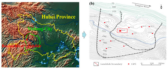
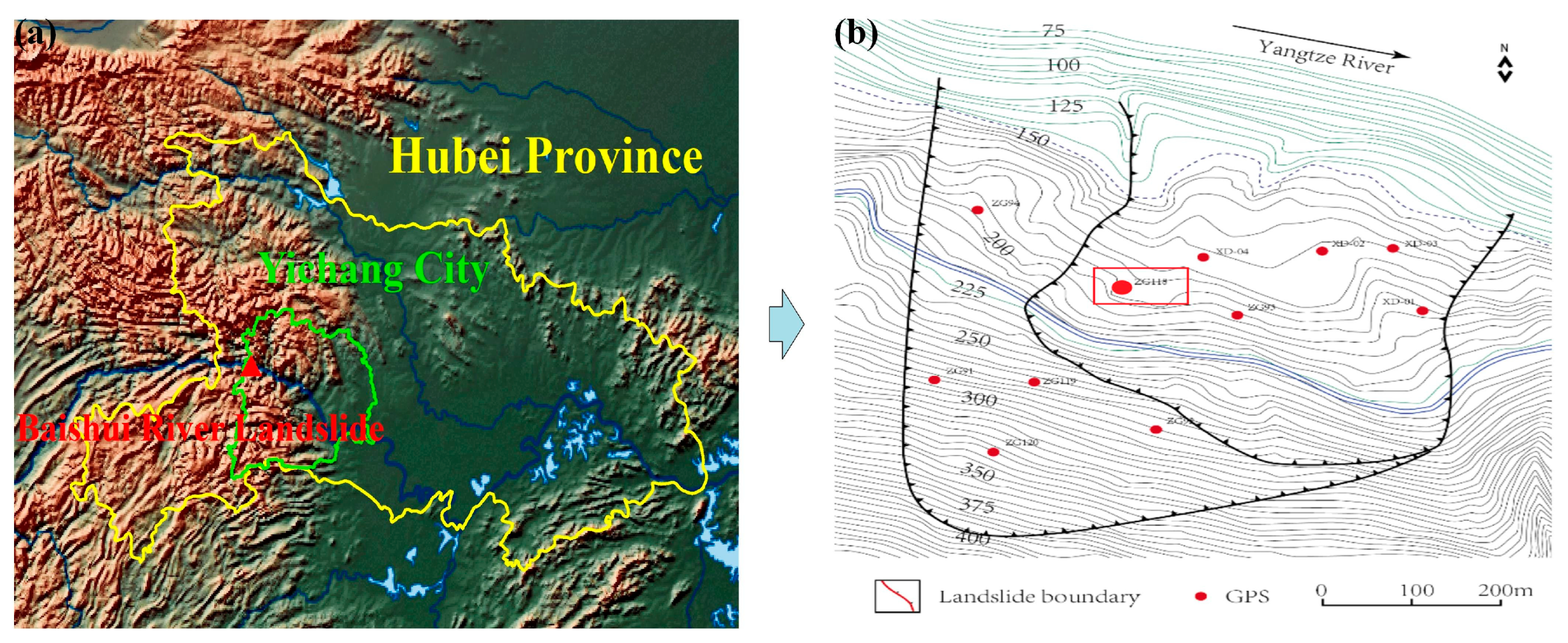
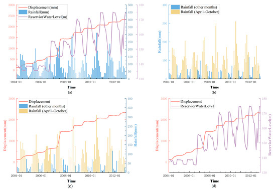
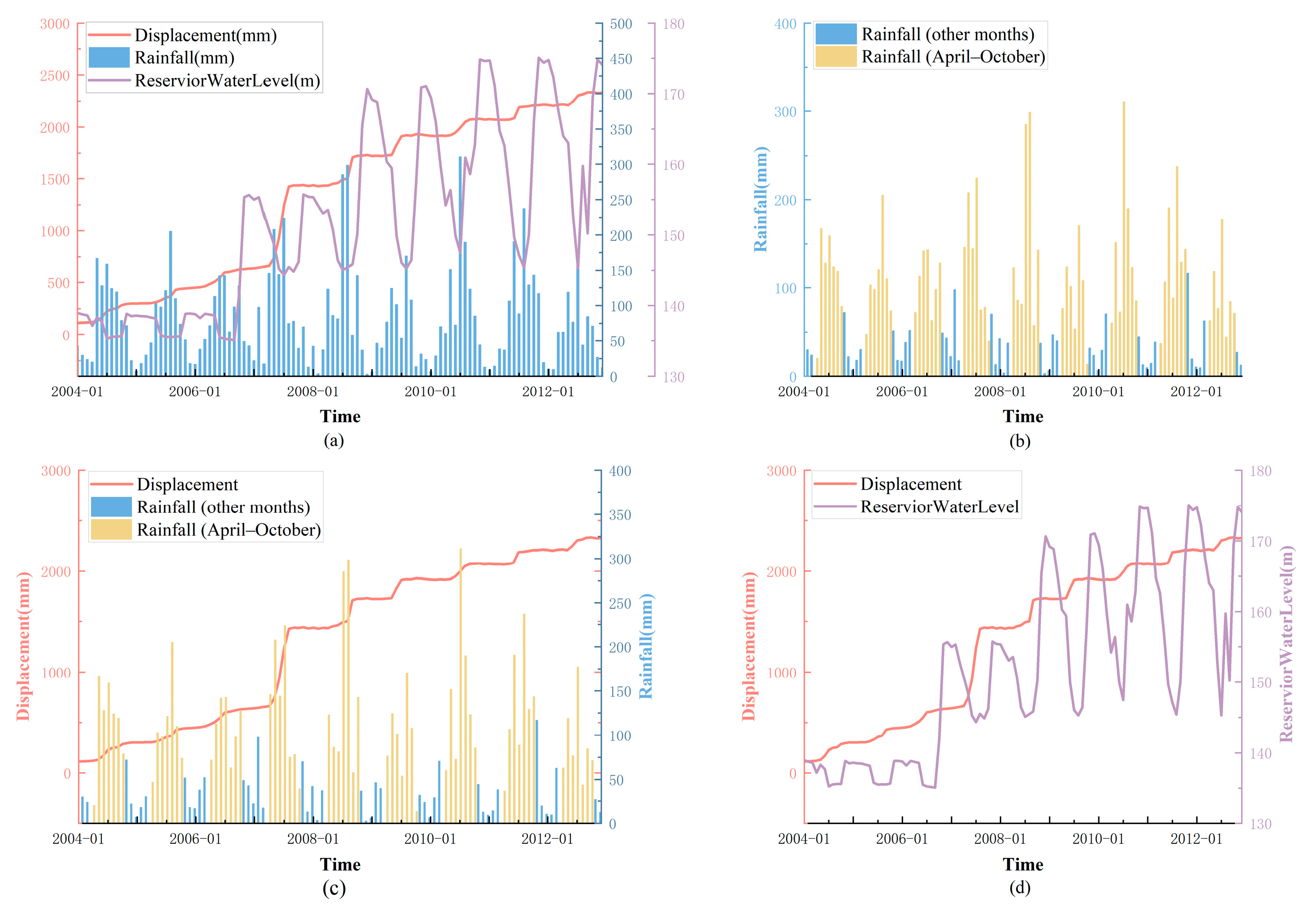
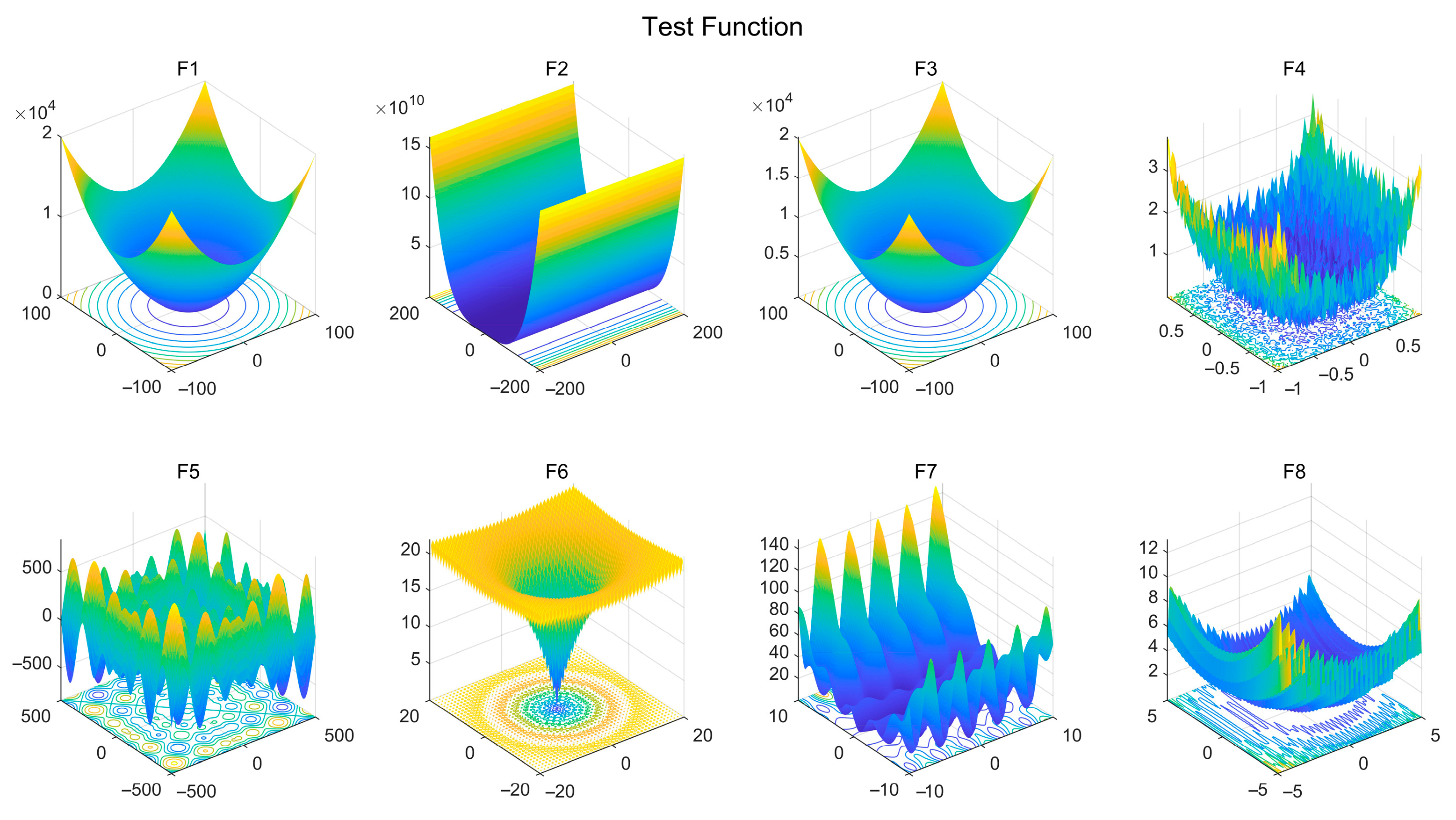
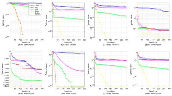
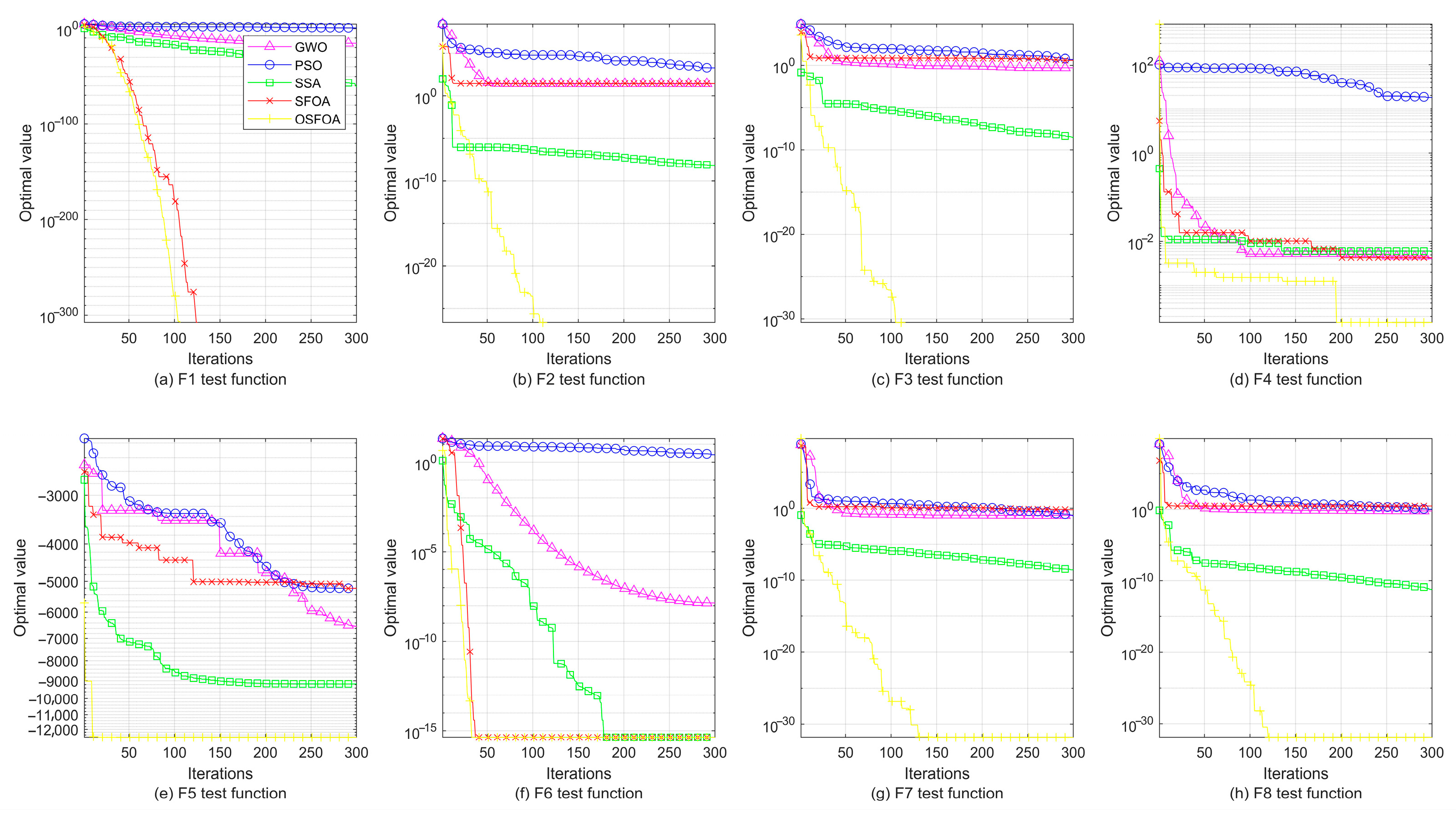
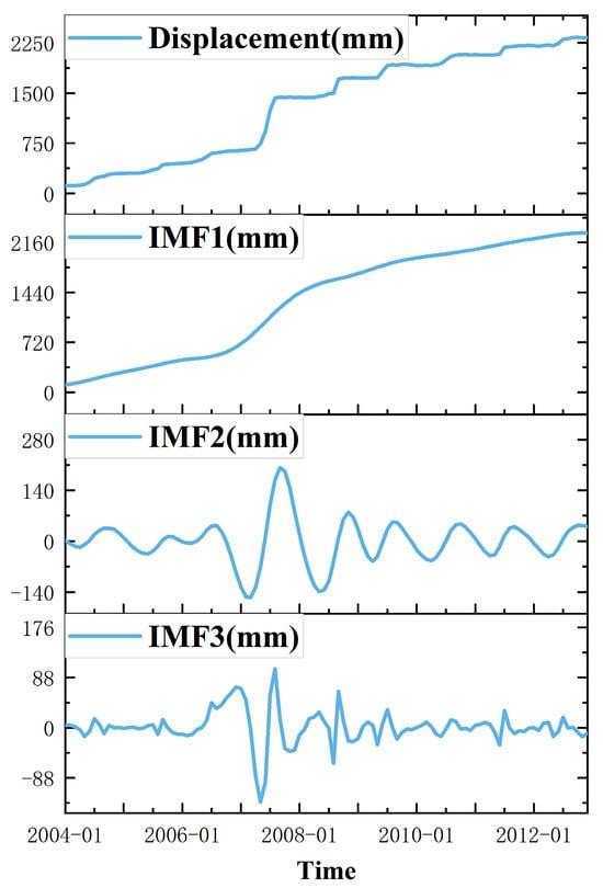
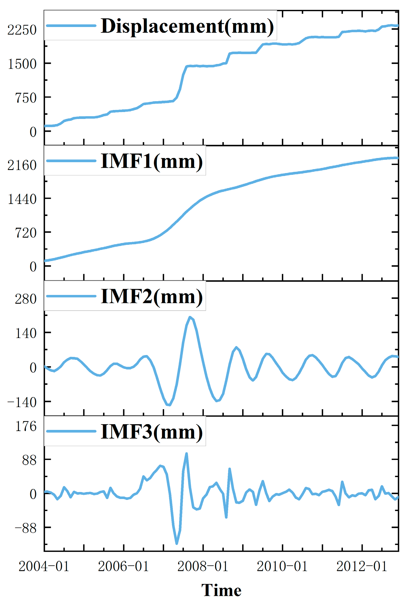
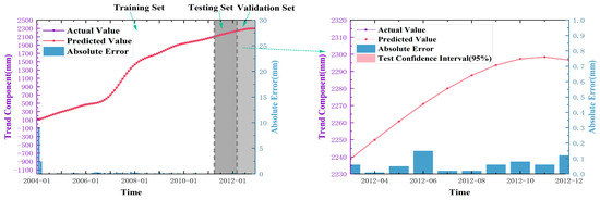
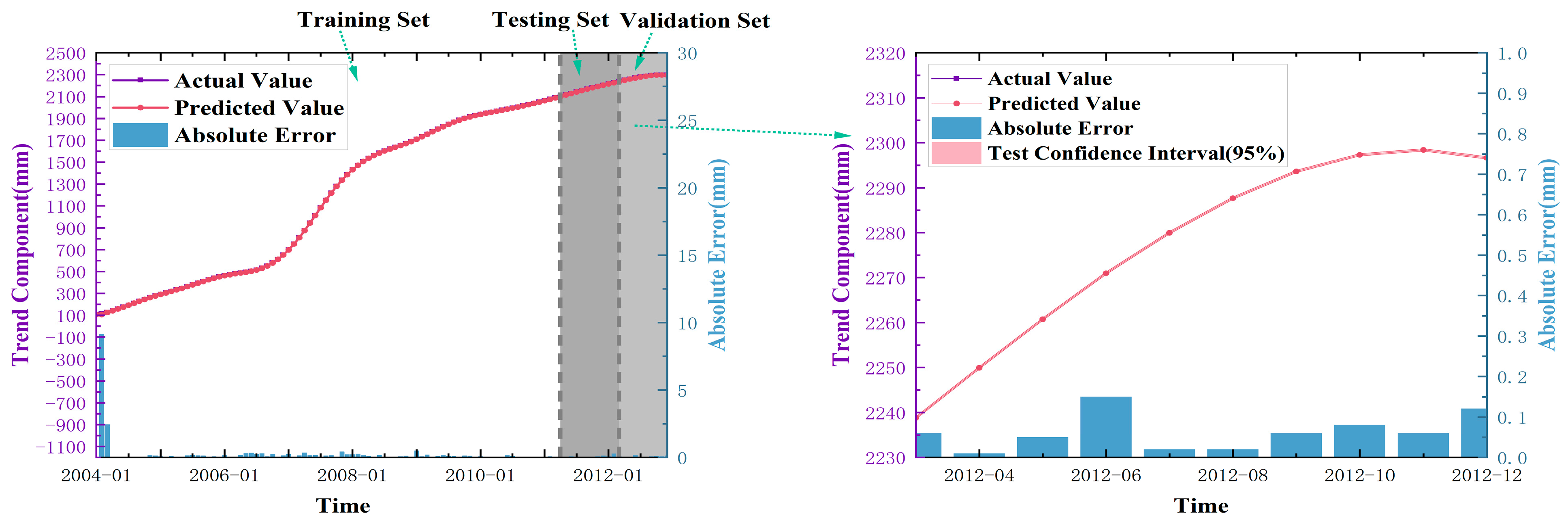
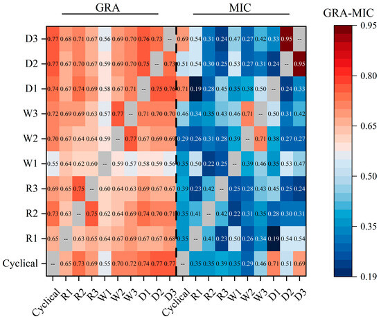
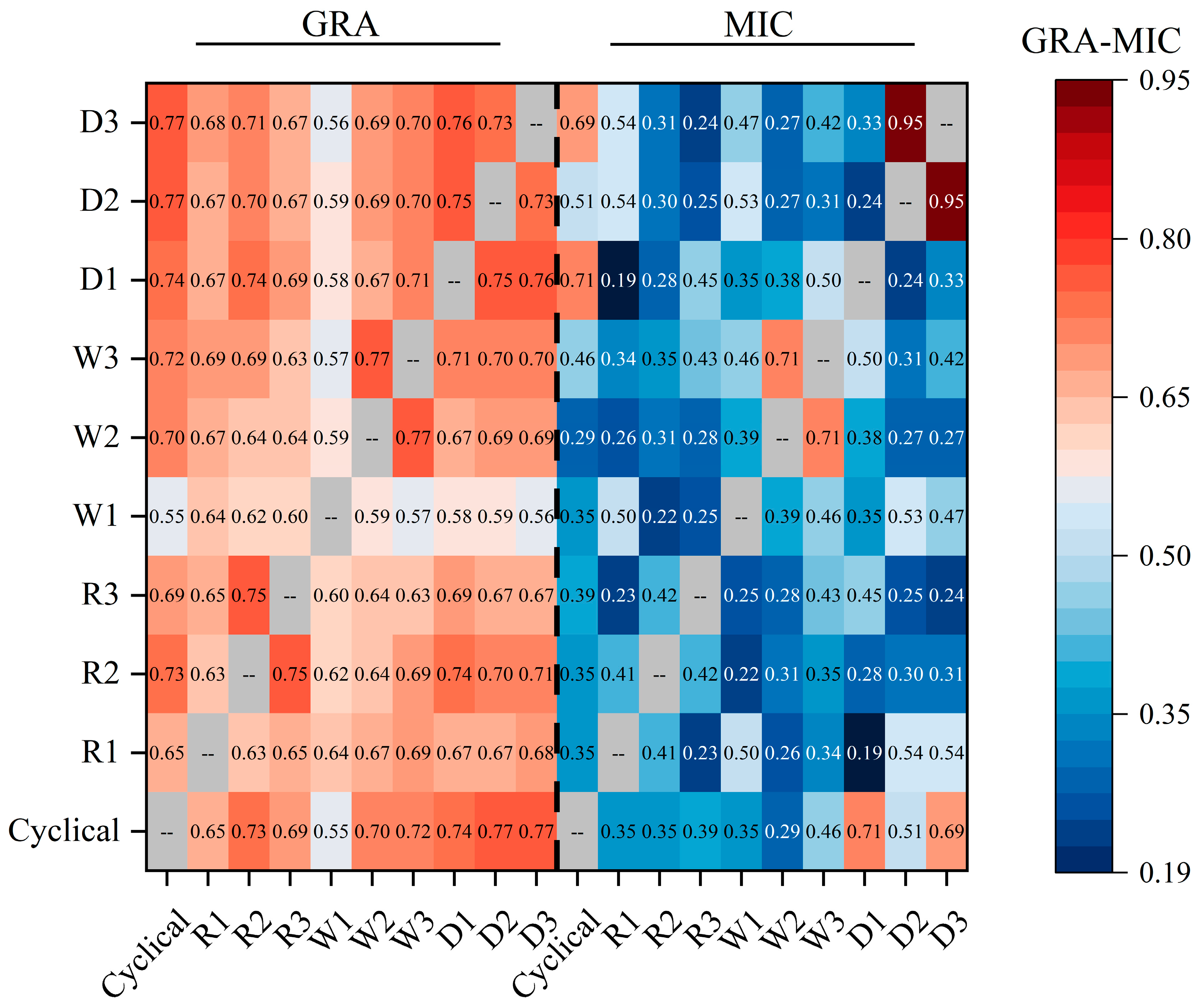
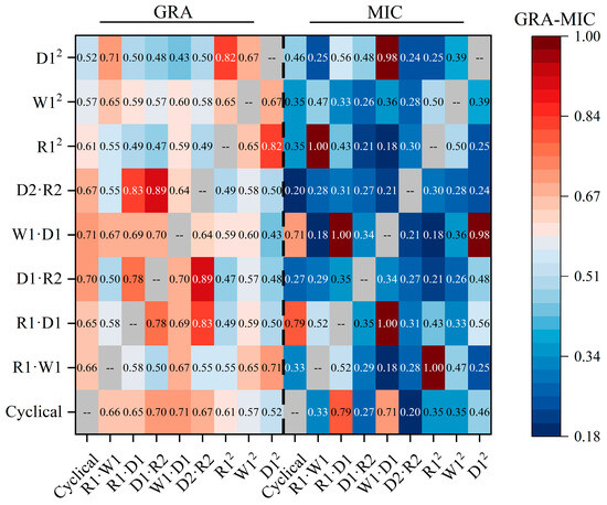
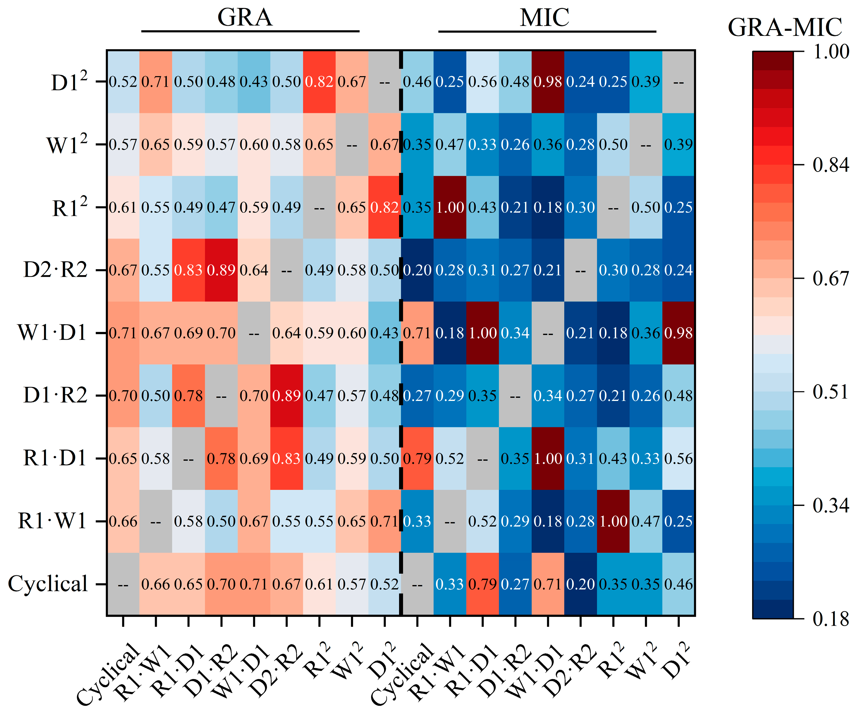
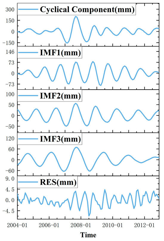
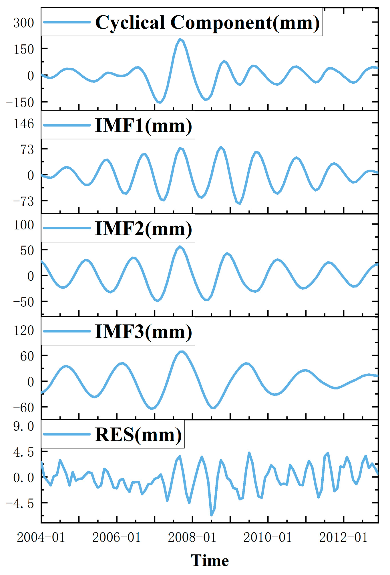
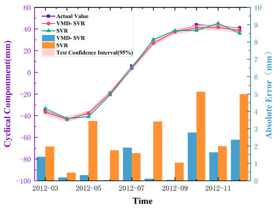
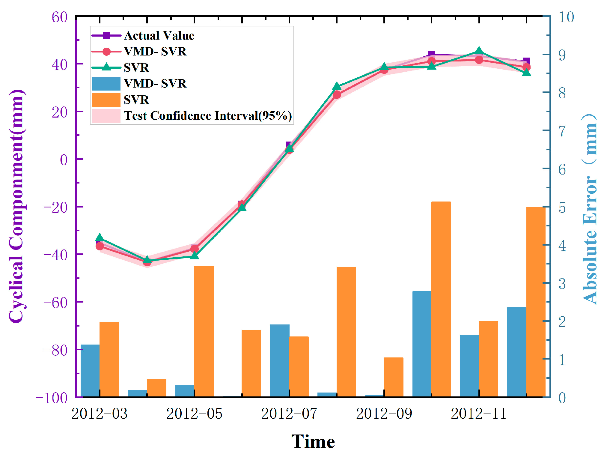
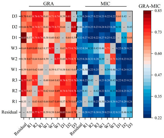
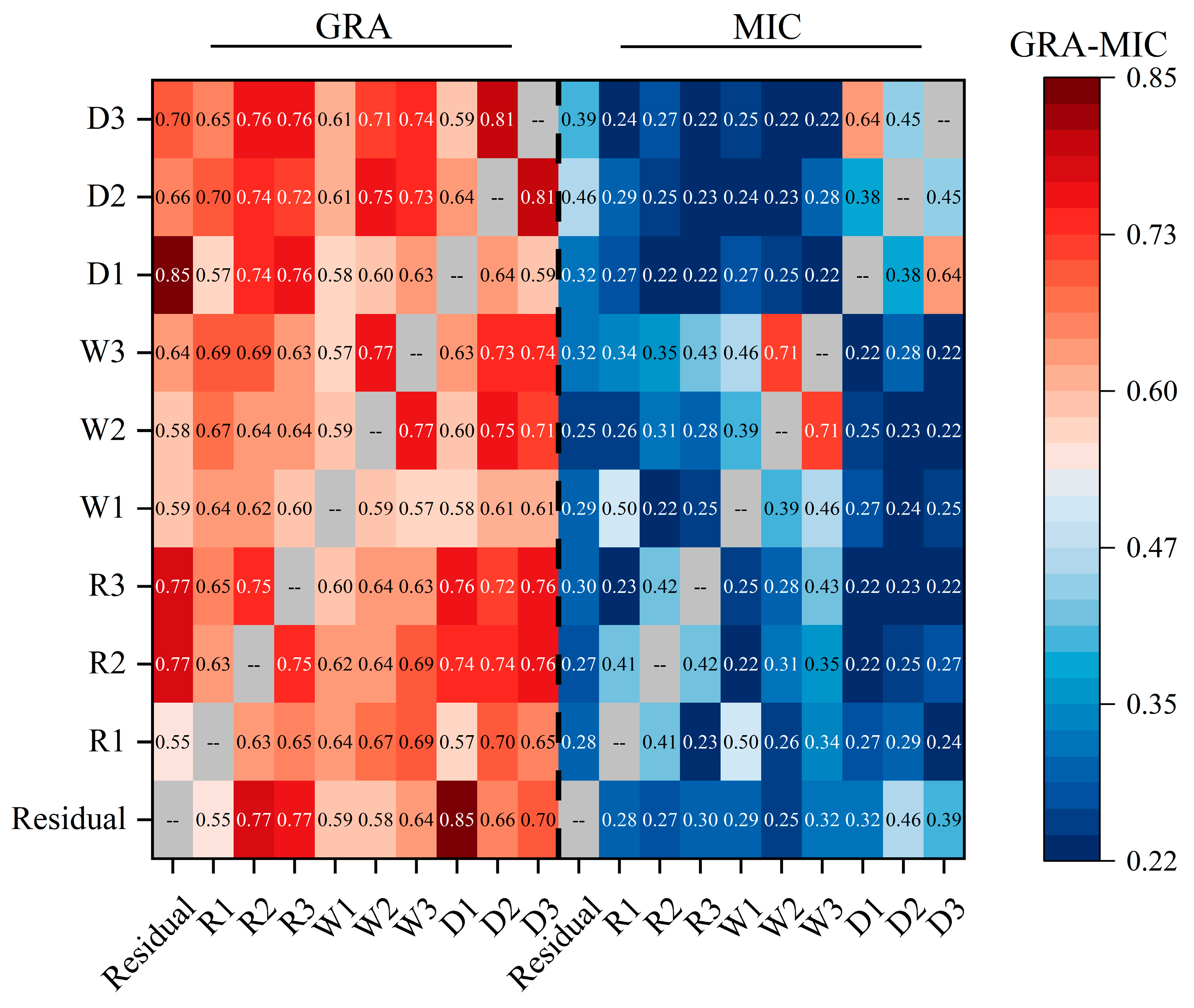
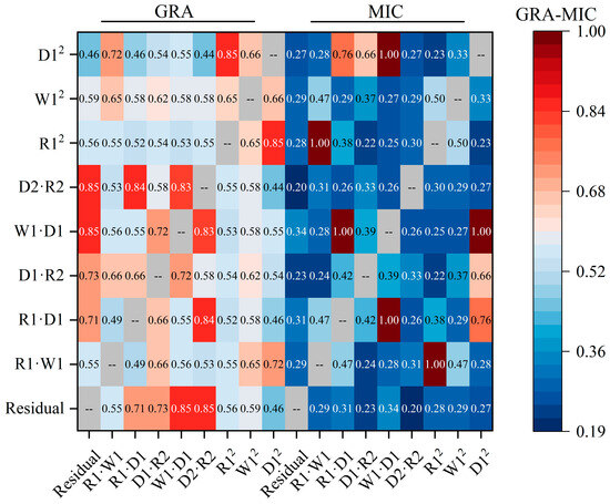
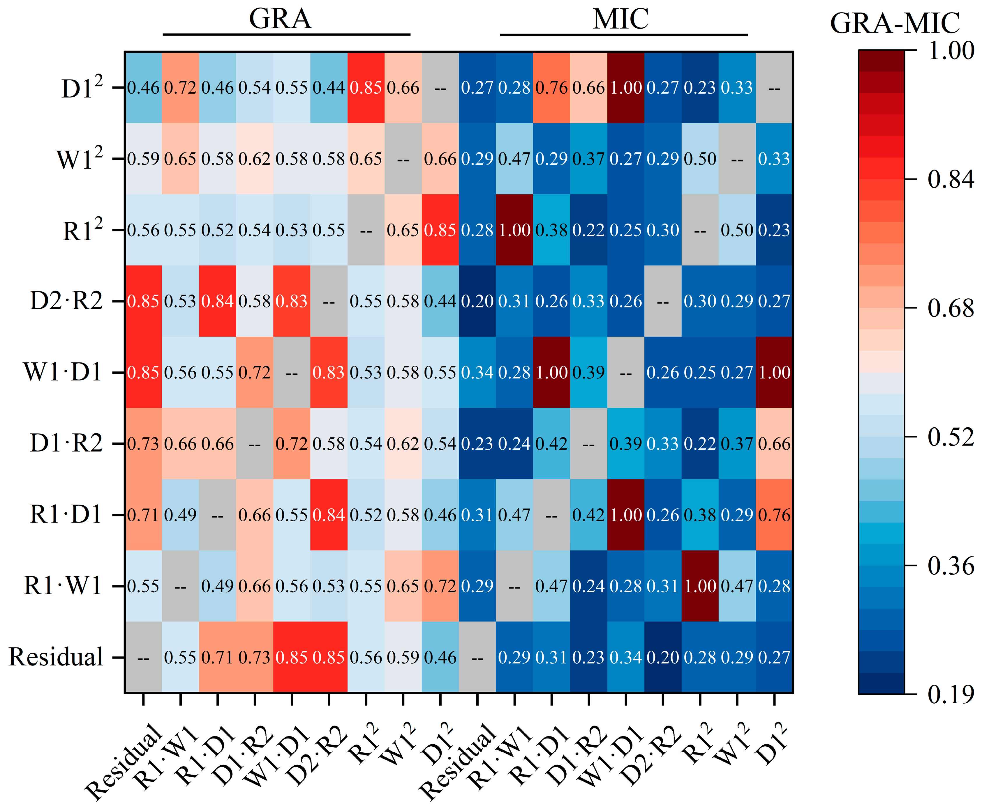
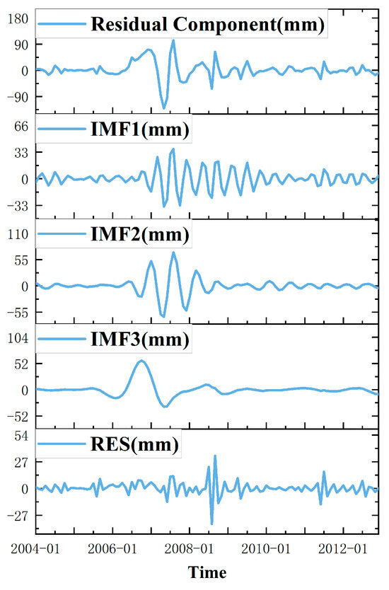
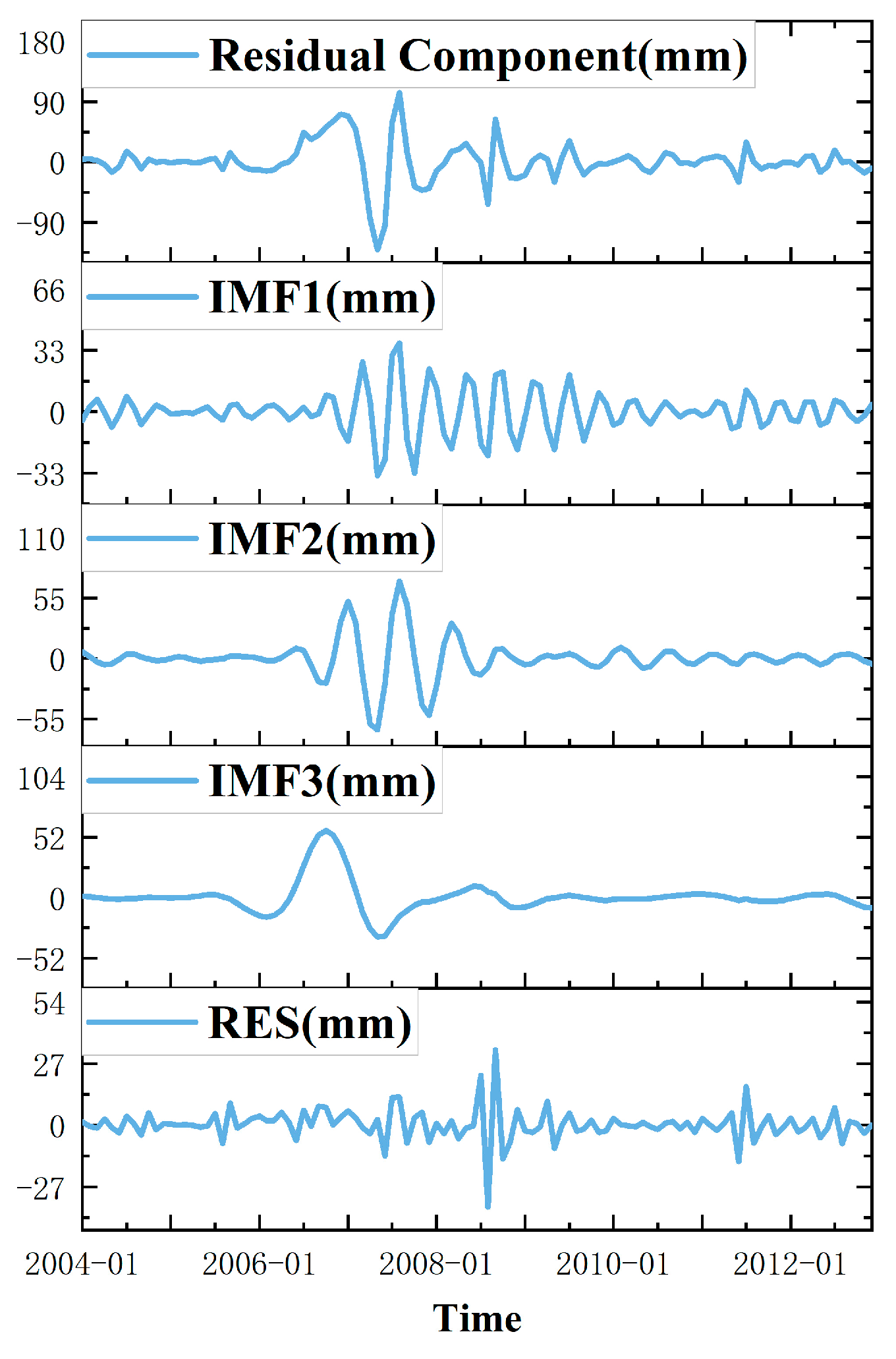
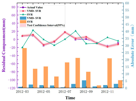
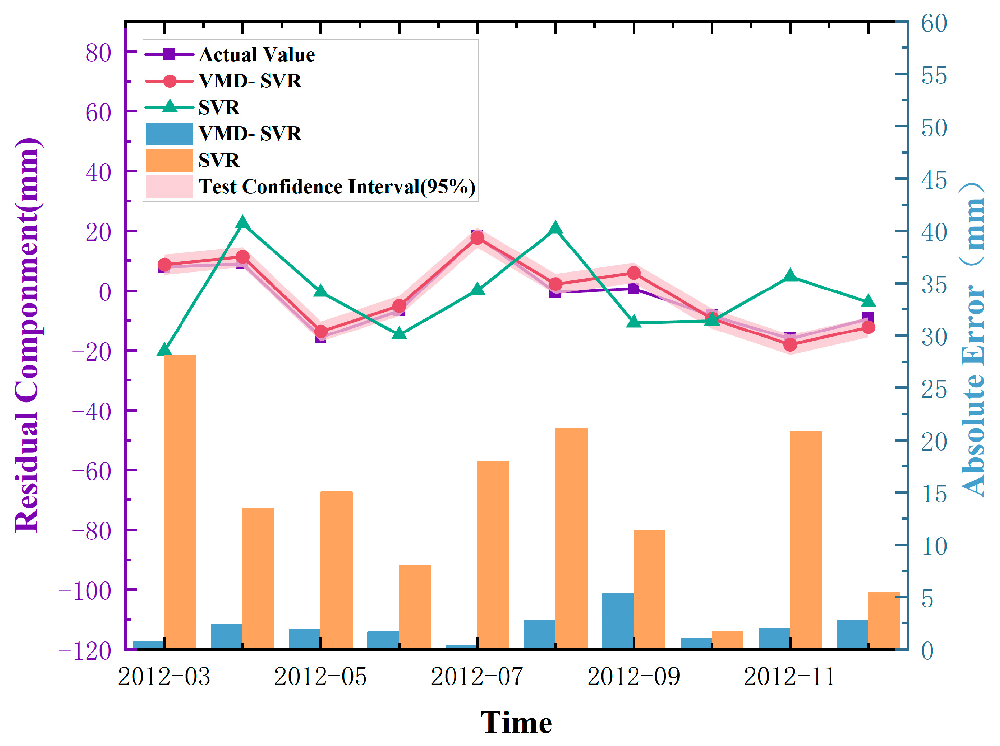
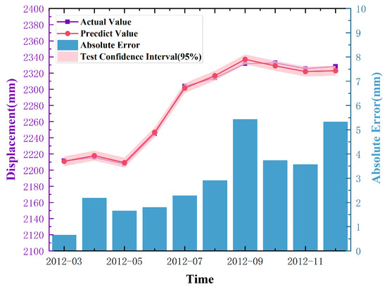
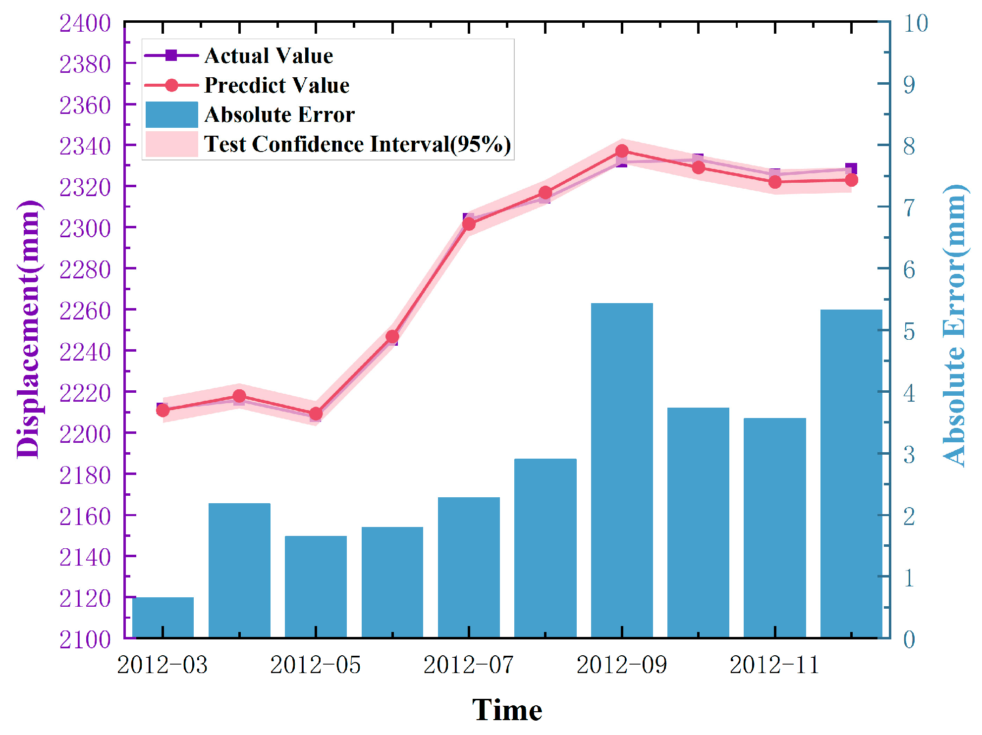
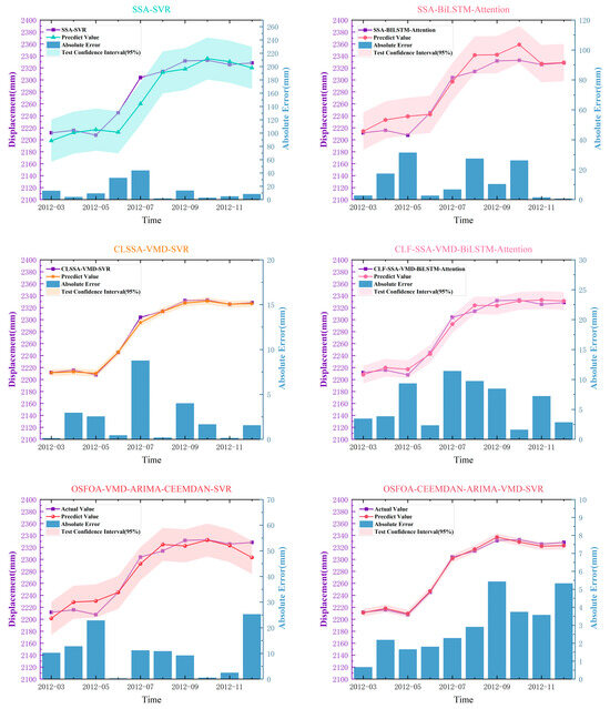
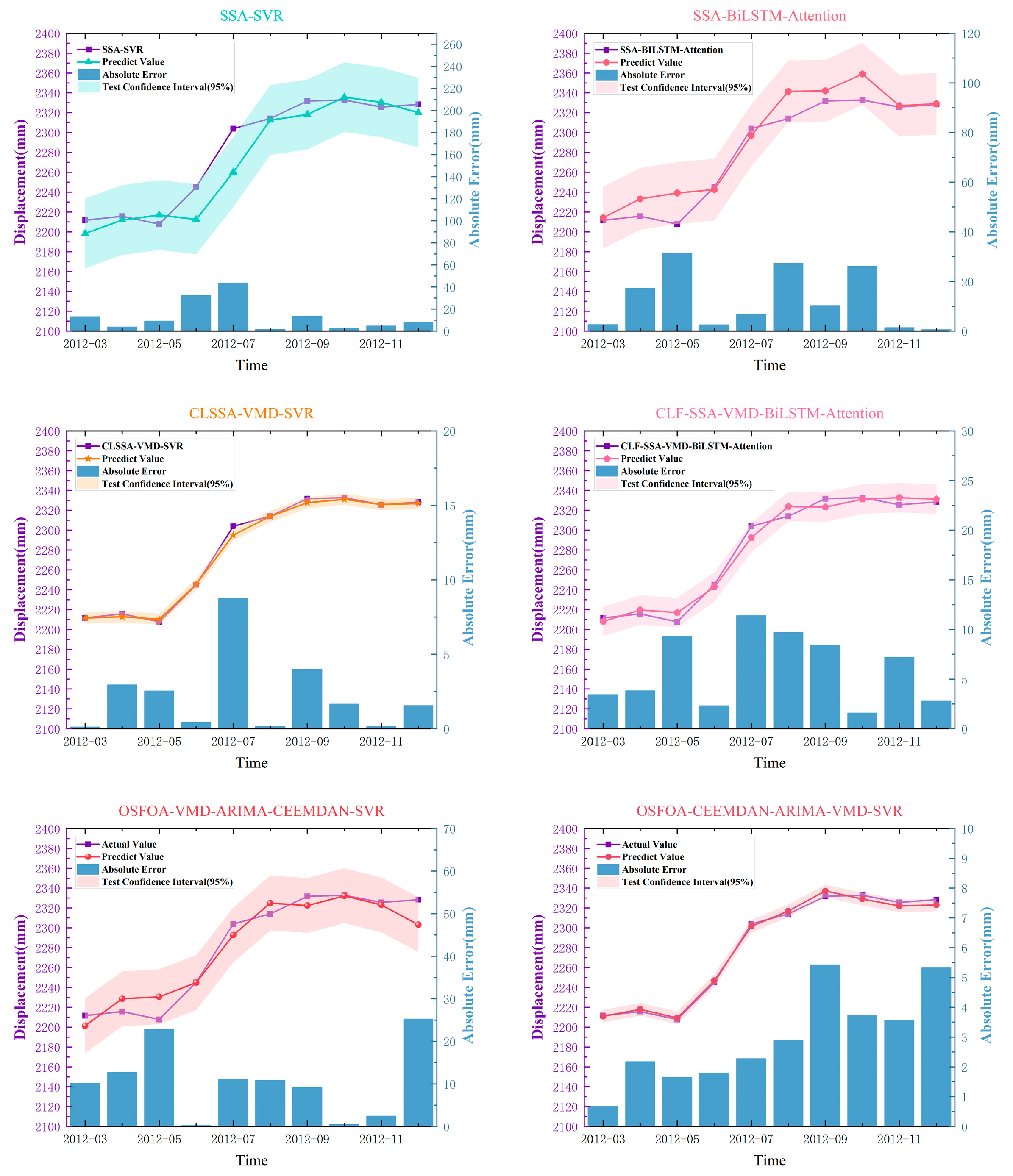
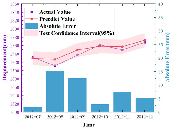
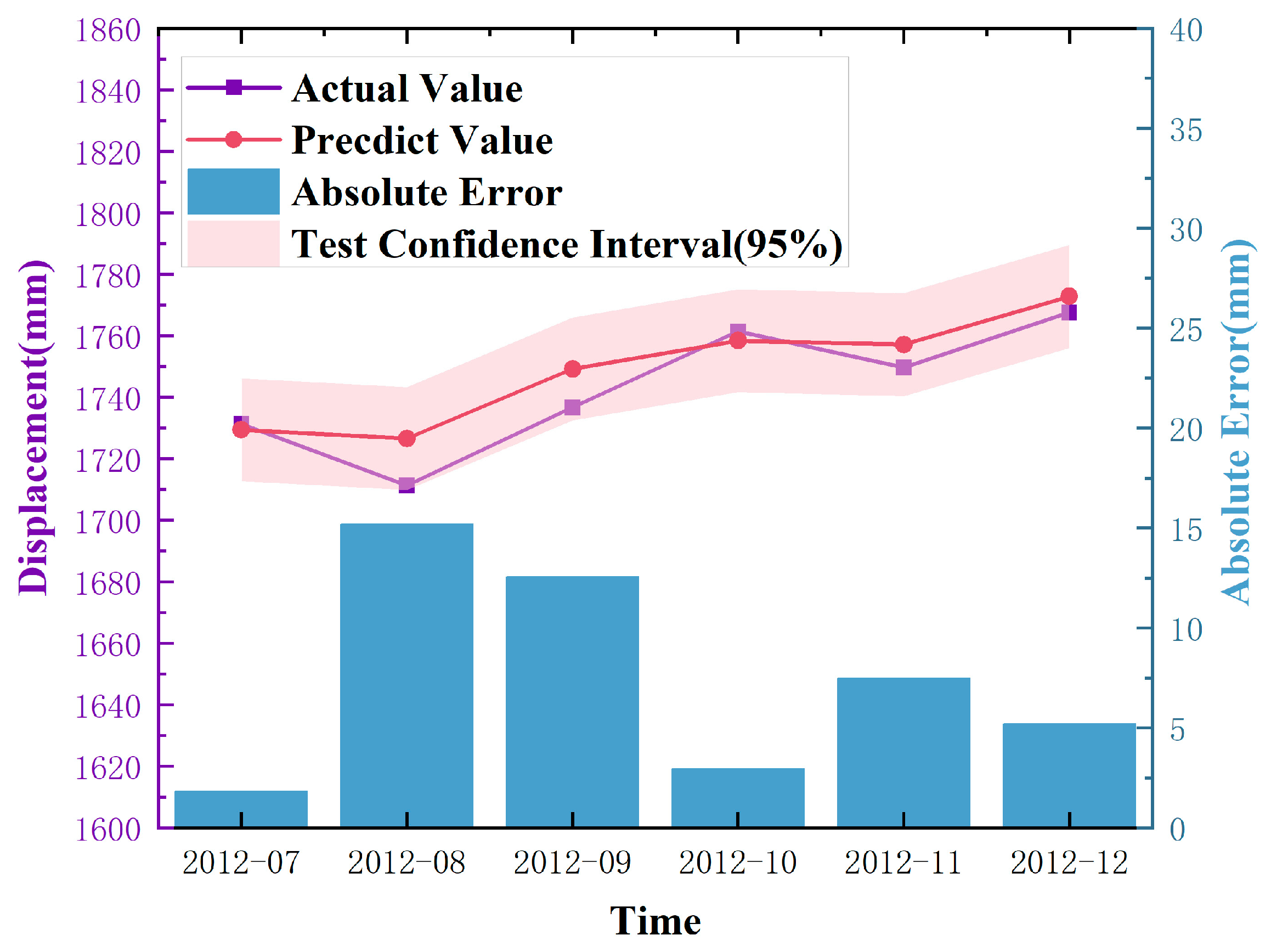

Disclaimer/Publisher’s Note: The statements, opinions and data contained in all publications are solely those of the individual author(s) and contributor(s) and not of MDPI and/or the editor(s). MDPI and/or the editor(s) disclaim responsibility for any injury to people or property resulting from any ideas, methods, instructions or products referred to in the content. |
© 2026 by the authors. Licensee MDPI, Basel, Switzerland. This article is an open access article distributed under the terms and conditions of the Creative Commons Attribution (CC BY) license.