Article

Comparison of PlanetScope and Sentinel-2 Spectral Channels and Their Alignment via Linear Regression for Enhanced Index Derivation

by
Christian Massimiliano Baldin
* and
Vittorio Marco Casella
Dipartimento di Ingegneria Civile e Architettura, Università degli Studi di Pavia, 27100 Pavia, Italy
*
Author to whom correspondence should be addressed.
Geosciences 2025, 15(5), 184; https://doi.org/10.3390/geosciences15050184
Submission received: 27 March 2025 / Revised: 13 May 2025 / Accepted: 14 May 2025 / Published: 20 May 2025

Abstract

:
Prior research has shown that for specific periods, vegetation indices from PlanetScope and Sentinel-2 (used as a reference) must be aligned to benefit from the experience of Sentinel-2 and utilize techniques such as data fusion. Even during the worst-case scenario, it is possible through histogram matching to calibrate PlanetScope indices to achieve the same values as Sentinel-2 (useful also for proxy). Based on these findings, the authors examined the effectiveness of linear regression in aligning individual bands prior to computing indices to determine if the bands are shifted differently. The research was conducted on five important bands: Red, Green, Blue, NIR, and RedEdge. These bands allow for the computation of well-known vegetation indices like NDVI and NDRE, and soil indices like Iron Oxide Ratio and Coloration Index. Previous research showed that linear regression is not sufficient by itself to align indices in the worst-case scenario. However, this paper demonstrates its efficiency in achieving accurate band alignment. This finding highlights the importance of considering specific scaling requirements for bands obtained from different satellite sensors, such as PlanetScope and Sentinel-2. Contemporary images acquired by the two sensors during May and July demonstrated different behaviors in their bands; however, linear regression can align the datasets even during the problematic month of May.

1. Introduction

1.1. Research Questions

Multispectral imagery [1], acquired from satellite sensors such as PlanetScope [2,3,4,5,6,7,8,9,10,11] and Sentinel-2 [12,13,14,15,16,17,18], provides essential data for observing and analyzing the Earth’s surface. Imagery acquisition through sensors at varied spatial and temporal resolutions necessitates rigorous comparative analysis to ensure data accuracy and consistency. Such validation facilitates the necessary alignment for their contemporary utilization, supplemented by interchangeable experience derived from comprehensive literature review. This paper presents a comparative analysis of PlanetScope and Sentinel-2 bands, focusing on contemporary acquisitions and the calibration of bands useful to correctly align soil and vegetation indices over the “Riserva San Massimo” [19,20] rice farm in Northern Italy before its computing. Previous research [2,3,4,11,21,22] has highlighted the importance of alignment between vegetation indices derived from PlanetScope and Sentinel-2 data, particularly during specific periods of the year. Building upon these findings, this study explores the application of linear regression as a technique to align individual bands before computing indices and investigate their shift in processed surface reflectance values [1]. This approach aims to enhance the comparability and reliability of data derived from these two satellite sensors.

1.2. PlanetScope and Sentinel-2: Key Factors

PlanetScope and Sentinel-2 have been widely studied during the last year [4,17,23,24,25,26] and a lot of new research papers have been published to assess PlanetScope’s capabilities to improve Sentinel-2 imagery and to be used on their own [6,15,23,27,28,29,30,31,32,33,34]. It has been demonstrated that PlanetScope is useful for multiple uses in precision agriculture [17,30,35], in land cover assessment, in change detection, in geology, and in various other fields. Previous research conducted by the same authors, which was documented in several papers [2,3,4], identified miscalibration issues within the Riserva San Massimo test site and outlined potential solutions [4]. The primary objective of the research was to leverage the Sentinel-2 experience of PlanetScope images to assess PlanetScope imagery for VRA precision agriculture in rice farming. PlanetScope provides significant improvements over Sentinel-2 in both spatial resolution (~3 m vs. 10 m best) and temporal resolution (~daily vs. 5 days). This makes it highly valuable for applications demanding fine spatial detail and very frequent monitoring. Sentinel-2 offers superior spectral resolution (more bands, including SWIR) and wider area coverage per pass (swath width), which is advantageous for broader-scale land cover classification, vegetation health assessments using specific indices (e.g., involving SWIR), and mineral mapping. Its data are also freely available.

1.3. Research Development

Previous research had shown that the Red, RedEdge, and NIR bands could be inconsistent during certain periods of the year [2,3]; however, calibration could be performed effectively even in the worst-case scenarios [4], demonstrating anyway which linear regression at the index level is not sufficient, particularly in relation to indices like NDVI and NDRE [2,3,4,11,21,22]. In order to conduct a more in-depth investigation, an analysis was performed utilizing five key spectral bands: Blue, Green, Red, RedEdge, and near-infrared (NIR). These bands were subjected to comparative assessment across two distinct temporal acquisitions, each featuring contemporaneous PlanetScope and Sentinel-2 imagery. One set of images exhibited low Root Mean Square Error (RMSE) [36], while the other demonstrated high RMSE. Subsequently, a linear regression analysis was applied to each of the five band pairings for both dates to evaluate the feasibility and efficacy of implementing calibration via linear regression. The focus on contemporary acquisitions allows for a more accurate representation of current conditions and minimizes the potential impact of temporal variations on the data. Analyzed bands are fundamental for calculating widely used vegetation indices such as NDVI [37,38,39] (Normalized Difference Vegetation Index), which measures the health and the vigor of vegetation, and NDRE [38,39] (Normalized Difference Red Edge Index), which is sensitive to chlorophyll content and can be used to assess plant stress. Additionally, these bands enable the computation of soil indices like Iron Oxide Ratio [40,41,42], which provides information about soil composition, and the Coloration Index [43,44], which can be used to identify different soil types. The outcomes of this research contribute to a deeper understanding of the scaling requirements for bands acquired from different satellite sensors. The study’s emphasis on linear regression [45,46,47] for band alignment [6,27,28,48] offers a potential solution for achieving greater accuracy and consistency in data derived from multispectral imagery [1]. This, in turn, can lead to more reliable and informed decision-making in various fields. For example, in agriculture, accurate and consistent data can be used to optimize irrigation and fertilization practices, leading to increased yields and reduced environmental impact [35,49,50,51,52,53,54,55]. In environmental monitoring, reliable data can be used to track changes in land cover and vegetation health, providing early warnings of potential environmental problems. In land use planning [15,56,57,58], accurate data can be used to make informed decisions about land development and conservation. In conclusion, precision fertilization [55], soil organic matter analysis [59], weed identification [60] and agricultural drought analysis [61], which require all spectral channels compared in this paper, can benefit from Remote Sensing analysis and improve future research and development efforts (like Time Series Analysis [62]) in Earth observation, potentially leading to the development of new and improved techniques for data analysis and interpretation.

1.4. Literature Review on Prominent Soil and Vegetation Indices Which Benefit Alignment

Prior investigations have focused on the alignment of indices such as Normalized Difference Vegetation Index (NDVI) [37,38,39,57,58,59,61,62,63,64] and Normalized Difference Red Edge (NDRE) [4,38,39,64,65,66] for primary use in precision agriculture [2,3,4,38,39]. This methodology is also extensible to other indices relevant to soil analysis, offering a broader scope of application. Spectral analysis has been extended to five bands to include other indicators: the Iron Oxide Ratio [17,40,41,42,64,67,68,69,70] and Coloration Index [43,59,60,71,72,73]. Table 1 provides a brief comparison, including the required spectral channels (bands).
The insights gained from this research emphasize the importance of considering specific scaling requirements for bands obtained from different satellite sensors like PlanetScope and Sentinel-2 [56,74].

1.5. Examples of Indirect Relationships Between Indices and Their Use for Revealing Information

NDRE outperforms NDVI in later growth stages and dense canopies, where NDVI tends to saturate. Although NDRE primarily measures vegetation health, it is indirectly influenced by soil properties, including moisture and organic matter. Soil texture, particularly fine particles like silt and clay, supports higher NDRE values due to better water and nutrient retention. Factors such as atmospheric conditions, soil background, and crop type must be considered for accurate interpretation of NDRE. While NDRE enhances understanding, it should be considered as one part of a larger set of data for comprehensive analysis. Indirect relationships with vegetation indices [75,76,77], like NDRE, can be utilized for many purposes, especially with ground truth and in correlation with other geological data: various factors in addition to geology, including climate, slope, aspect, and human activity, affect vegetation, requiring the integration of extensive data. Rocks type can influence vegetation [78] and NDRE values: areas with consistently lower NDRE might indicate nutrient-poor soils [79] derived from rocks like granite or quartzite. Areas with consistently higher NDRE (within the same vegetation type) could suggest more fertile soil [80] derived from rocks like basalt or shale. Sharp boundaries in NDRE patterns, especially if they align with known geological contacts or lineaments, can be suggestive of changes in rock type. Mineralization Zones [40,42,81,82] can influence NDRE (through plant stress): some types of mineralization (e.g., copper, zinc, gold deposits) can lead to elevated concentrations of heavy metals in the soil. These heavy metals can be toxic to plants, causing stress and altering their chlorophyll content. Areas with anomalously low NDRE values, particularly if they occur within a relatively uniform vegetation type and are localized, could be indicative of plant stress due to heavy metal contamination. The Red Edge region is particularly sensitive to changes in chlorophyll content, making NDRE potentially more sensitive to this type of stress than NDVI [38,39]. Mapping Alteration Zones [82,83] could be carried out through analyzing NDRE variations: hydrothermal alteration [82,84], a process associated with certain types of ore deposits, can modify the mineral composition of rocks, often resulting in the formation of clay minerals and other alteration products. These altered rocks frequently exhibit different weathering characteristics and soil properties compared to unaltered rocks. NDRE can be used to identify drainage patterns and soil moisture [85] because vegetation typically flourishes in regions with elevated soil moisture, such as along drainage channels or areas with shallow groundwater. Higher NDRE values can sometimes reveal drainage patterns, as denser and healthier vegetation along watercourses will exhibit a higher NDRE signal [86]. This phenomenon can assist in delineating geological structures that govern drainage, such as faults and fractures. Additionally, areas of consistently higher NDRE within relatively uniform terrain may indicate zones of elevated soil moisture, potentially influenced by geological factors such as impermeable layers or springs. Although topography and other elements significantly impact drainage [78], NDRE alone is not a definitive indicator of subsurface geology but rather provides valid clues. NDRE can also be used to monitor surface disturbances and reclamation: mining activities, landslides, and other factors can significantly transform the soil cover, frequently leading to vegetation loss. By employing NDRE in a multitemporal context [58] (comparing images of the same region at different time points), it is feasible to observe alterations in vegetation, which serve as indicators of the extent of disturbances. Iron oxides (like hematite and goethite) have strong reflectance in the red portion of the spectrum and low reflectance in the blue: this is relevant in a fertilization/herbicide context. This ratio highlights areas with iron oxide concentrations, which are common in many geological environments, including weathered rocks, gossans (indicators of sulfide mineralization), and certain types of soils. It is a simple but effective way to identify potential areas of iron mineralization [81]. This ratioing technique is particularly valuable as it helps to mitigate the effects of illumination differences that can arise due to variations in terrain and shadowing. By normalizing the data in this way, the relative spectral differences between the red and blue reflectances, which are more indicative of the surface material composition, are enhanced. CI is used to delineate zones with different colors. In a geological setting, it can be used to differentiate rocks or areas with distinct colors, for instance, related to iron oxides. The Coloration Index serves as a valuable tool in geological remote sensing for the differentiation of rock types based on color variations (and search for hematite/geothite) [59]. Its principle lies in exploiting the differential reflectance of geological materials in the visible spectrum, with positive values often indicating the presence of iron oxides. Currently, the Coloration Index plays a significant role in preliminary geological surveys, mineral exploration (especially for iron), and soil studies [59,60,71,72,73]. Case studies demonstrate its utility in mapping iron-rich zones using various satellite and airborne sensors.

1.6. Evaluation of Band Calibration Through RMSE and MAE

Image processing algorithms are commonly evaluated using the Root Mean Square Error (RMSE) and the Mean Absolute Error (MAE) metrics [36].
RMSE is a widely used metric for evaluating the accuracy of predictions or measurements. When RMSE is assessed globally by analyzing it pixel by pixel for a single band, each pixel’s error is calculated by comparing the values from each sensor. The errors are then squared, averaged, and the square root of this average is taken to obtain the RMSE. This process ensures that large errors have a greater influence on the RMSE value, making it an effective measure of overall accuracy. This metric is particularly useful for identifying pronounced deviations in image datasets.
MAE quantifies the average magnitude of errors in a set of predictions, without considering their direction (i.e., whether they are positive or negative). The MAE is determined by computing the average of the absolute differences between predicted values and actual values. Due to the fact that it does not involve squaring the error terms, large errors do not disproportionately influence the MAE. This attribute renders MAE particularly valuable in datasets containing outliers that are not necessarily indicative of the model’s overall performance, as observed in this application. In Formulas (1) and (2), PS_Band(i,j) represents each pixel in the specified position (i,j) within the matrix of pixels for PlanetScope’s band; similarly, S2_Band(i,j) denotes each pixel in the specified position (i,j) within the matrix of pixels for Sentinel-2’s band.
R M S E B a n d = 1 n i , j P S _ B a n d i , j S 2 _ B a n d i , j 2 )
M A E B a n d = i , j P S _ B a n d 2 i , j S 2 _ B a n d 1 i , j n
RMSE and MAE are essential metrics in this research, evaluated for each pair of images, with RMSE focusing on the magnitude of significant errors and MAE providing an equitable assessment of average error magnitude. Both metrics are crucial for a thorough understanding of algorithm performance and error distribution in image processing tasks.

2. Materials and Methods

2.1. Riserva San Massimo Test Site

The “Riserva San Massimo” [19,87,88,89,90], located in Gropello Cairoli (PV), within the Lombardy Park of the Ticino Valley, represents a notable example of integrating environmental conservation with sustainable agriculture. Figure 1 illustrates maps framing the rice farm in Italy (1a) with its varieties (1b). Reference system used: WGS84 UTM-32N.
Classified as a Site of Community Importance (SCI IT2080015) [91] and partly as a Special Protection Area (SPA) [92], the reserve covers approximately 800 hectares. It includes wetland forests (particularly black alder), natural springs, water meadows, and agricultural fields primarily used for cultivating authentic Carnaroli rice. The rice varieties grown include Cammeo, LunaCL, Rosa Marchetti, and Vialone. This research was conducted in collaboration with the esteemed agronomic consulting team led by Dr. Agr. P.A. Barbieri and Dr. Agr. G.L. Rognoni [93,94], who oversees the rice farming operations for the reserve, providing numbered crops as used for field management (with their borders and variety): essential knowledge which validates this work belongs to their experience and research activities with “Ente Risi” [95]. This site exemplifies successful sustainable agriculture and ecological preservation. The implementation of Variable Rate Application (VRA) technology optimizes the distribution of fertilizer, leading to cost reduction, decreased environmental impact, and potentially improved crop yields. This research pertains directly to the enhancement of the fertilization process for the “Riserva San Massimo” rice farm, which has been consistently monitored over the years using Sentinel-2 data by the agronomic consulting team referenced above. The farm now seeks further improvement through the utilization of PlanetScope imagery, owing to its superior spatial and temporal resolution.

2.2. Variable Rate Application to Precision Farming at “Riserva San Massimo”

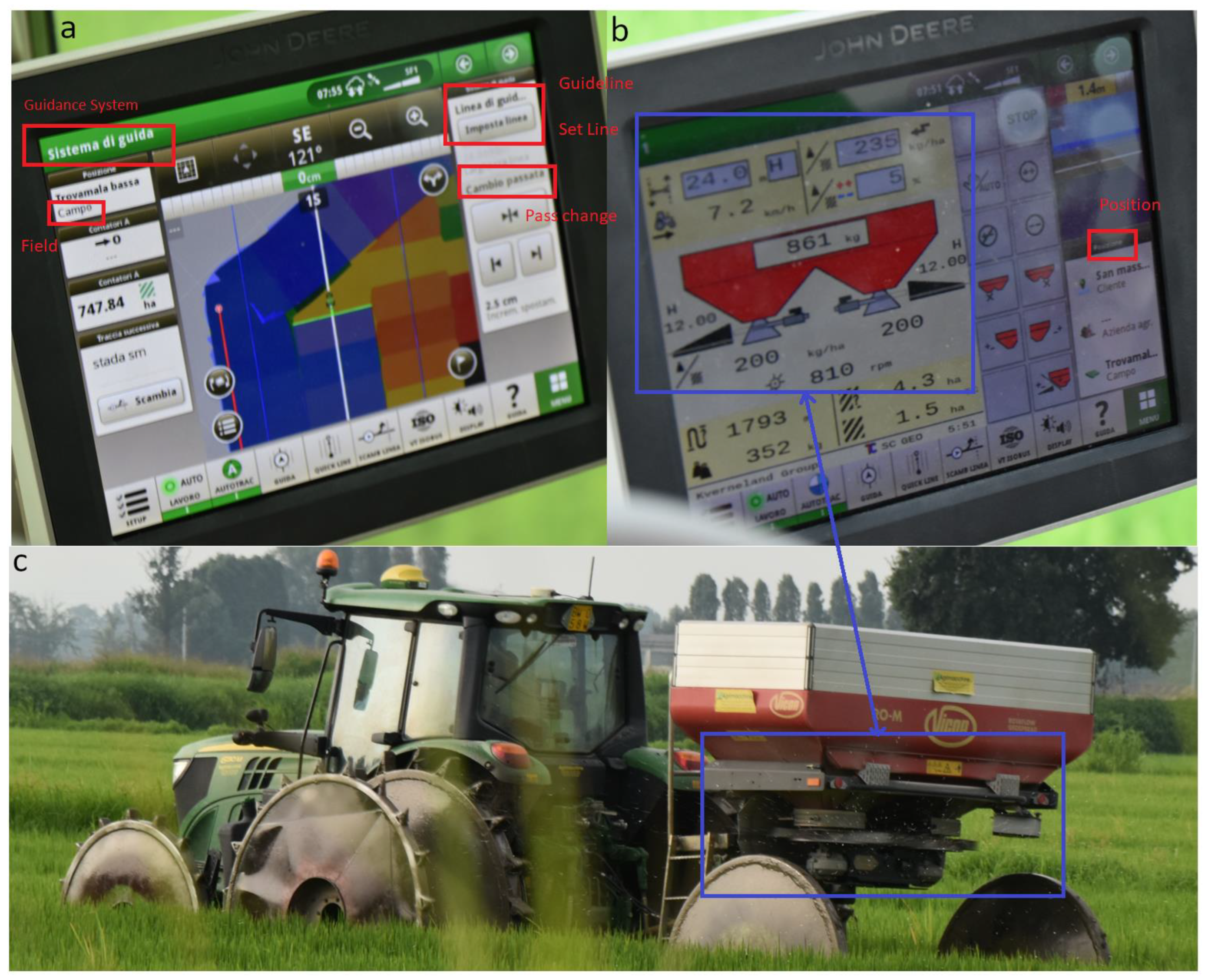
During fertilization (Figure 2), a specialized fertilizer spreader (Figure 2c) is used, interfaced with hardware that manages the tractor’s semi-autonomous driving capabilities (Figure 2a,b). The spreader accurately disperses granular fertilizer according to the prescription map (Figure 2a), which details the specific dosage for each section of the field.
This precise calibration ensures maximum deviations of only 1% from the prescribed amounts provided by the agronomist. This implementation of Variable Rate Application (VRA) technology proves its effectiveness in precision agriculture, enabling the careful application of fertilizers and thereby optimizing crop yields, reducing costs, and minimizing environmental impact. The main frame (Figure 2a) displays the prescription map, where different colors indicate varying requirements (blue signifies no additional fertilizer needed, for example). By following the prescribed path, the exact amount of fertilizer can be applied to each tile.
This fieldwork is closely associated with the ability to create accurate prescription maps, as the 1% error rate demonstrates that the more precise a prescription map is, the better the results will be. Transitioning to higher spatial resolution reduces edge effects and ensures the precise distribution of fertilizer. By leveraging Sentinel-2 data and calibrating PlanetScope bands to match Sentinel-2, the accuracy of derived indices is enhanced, thereby improving the effectiveness of chemical product applications. The observations captured in the images demonstrate the effective management of crop tillering, a practice guided by the expertise of the managers and field workers at “Riserva San Massimo” rice farm.

2.3. Sentinel-2

The Copernicus Sentinel-2 project [12,13,14,16,18,96,97,98,99] utilizes two polar-orbiting satellites, Sentinel-2A and Sentinel-2B, which are positioned in sun-synchronous orbits 180° apart. Recently, Sentinel-2C has become operational [98]. The Sentinel-2 mission offers high-resolution optical imagery in 13 spectral bands via Multispectral Instruments (MSI). Imagery resolution ranges from 10, to 20 to 60 m. Sentinel-2 images are processed into two types: top of atmosphere (TOA), affected by atmospheric conditions, and bottom of atmosphere (BOA), which shows surface reflectance without atmospheric interference. The MSI [12,13,100,101] captures data across visible, near-infrared (NIR), and shortwave infrared (SWIR) bands, providing detailed and accurate Earth observations with a revisit time of 5 days for most global regions.
Use of Sentinel-2 [102] images is under license: Copernicus Sentinel satellite—Open Access compliant, CC BY-SA 3.0 IGO

2.4. PlanetScope

Planet Labs operates the PlanetScope [5,6,7,8,9,10,103] constellation of over 200 Earth observation satellites called Doves and SuperDoves [104,105,106]. These satellites capture images of the Earth’s surface at a 3 m resolution. SuperDove sensors capture 8-band images used in this research, which include surface reflectance data and rectified data. PlanetScope provides almost daily revisit times, enabling frequent and consistent monitoring of the Earth’s surface. Use of PlanetScope [107] images is under license: ©Planet Labs PBC, CC BY-NC-SA 2.0

2.5. Choice of Images

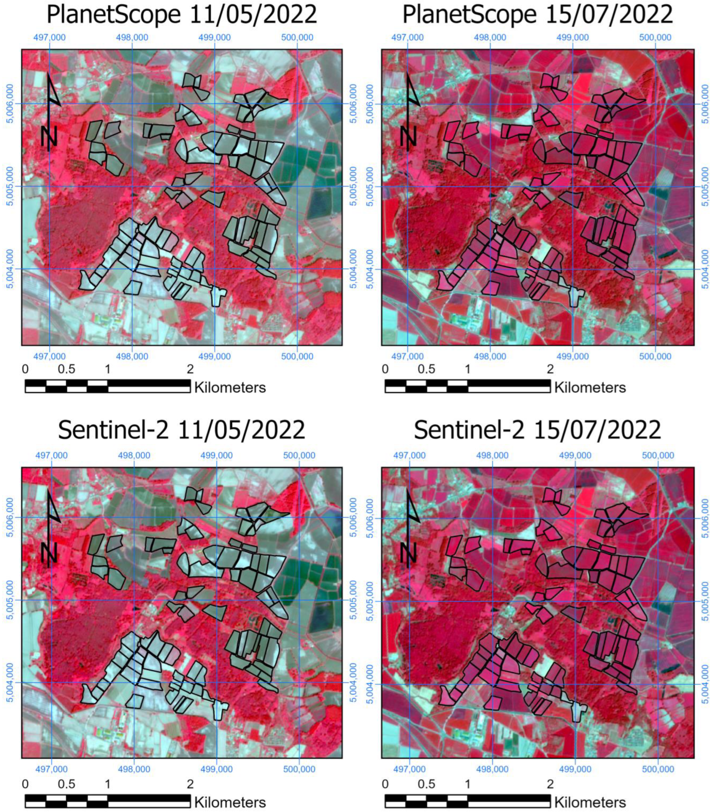
Figure 3 represents a detailed view of some rice crops (through standard colors, RGB images) for the dataset used: PlanetScope [7] (spatial resolution 3 m) and Sentinel-2 [108] (spatial resolution 10 m at its best as in the figures) contemporary acquisitions for dates 11 May 2022 (Sentinel-2 at 10:16, PlanetScope at 10:13) and 15 July 2022 (Sentinel-2 at 10:15, PlanetScope at 9:53). Notably, for the first date, images were captured at intervals of 3 min, while for the second date, they were taken at intervals of 22 min. This allows for a comparison of images with similar lighting, which is crucial for the radiometric approach. The reference system used is WGS84 UTM-32N. From the agronomist’s experienced perspective, the timeframes chosen are associated with the rice growth stage (mixed bare soil and sparse vegetation) in May and with full vegetation coverage (fertilization) in July.
These images use standard color bands: Blue, Green, and Red.
  • Sentinel-2: B2 (Blue): 492.7 (65) nm; B3 (Green): 559.8 (35) nm; B4 (Red): 664.6 (30) nm. All these bands have 10 m of spatial resolution.
  • PlanetScope: Band 2 (Blue): 490 (50) nm; Band 4 (Green): 565 (36) nm; Band 6 (Red): 665 (31) nm. All these bands have 3 m of spatial resolution.
Color Infrared images (CIR) [109] in Figure 4 highlight sparse vegetation coverage during May and full vegetation coverage during July with strong red color over rice crops.
Sentinel-2 images, Level-2A products, exhibited the following attributes: atmospherically corrected surface reflectances in cartographic geometry. Granules were ortho-images in UTM-32N/WGS84 projection. PlanetScope images, acquired by Superdove Sensor, exhibited the following attributes: 8 bands, calibrated surface reflectance [112], rectified assets, and radiometrically harmonized with Sentinel-2 [9,23,103]. In previous research [4] (paragraph 2.4), the harmonization of PlanetScope with Sentinel-2 was discussed: the Red, Green, Blue, and near-infrared bands of PlanetScope sensors are harmonized and normalized to align with those of Sentinel-2 (RedEdge is not harmonized). As demonstrated in this paper, it is, however, essential to ensure the alignment of harmonized bands. PlanetScope also utilizes UTM-32N/WGS84 projection. Images were selected through an extensive study spanning three years (2021–2023). The analysis of images to identify the optimal pair of multispectral images from Sentinel-2 included 73 images for 2021, 71 images for 2022, and 73 images for 2023. Similarly, for PlanetScope, the analysis comprised 222 images for 2021, 345 images for 2022, and 739 images for 2023. Several images were identified as dates on which concurrent acquisitions by Sentinel-2 and PlanetScope occurred. Through detailed research and analysis [2,4], it was found that the RMSE, applied to images pixel by pixel, varies over different timeframes. In some periods, indices showed similar values (low RMSE in July, during fertilization), while in other periods, RMSE was very high, indicating significant differences between images (high RMSE in May). This phenomenon was examined using two datasets from different dates representing each case. Previous research [2,3,4,11] indicated that aligning indices directly is feasible but does not provide insights into the underlying causes. The solution involves aligning bands directly to understand previously undiscovered differences.

2.6. Band Alignment Through Linear Regression and Nearest Neighbor Sentinel-2 Oversampling

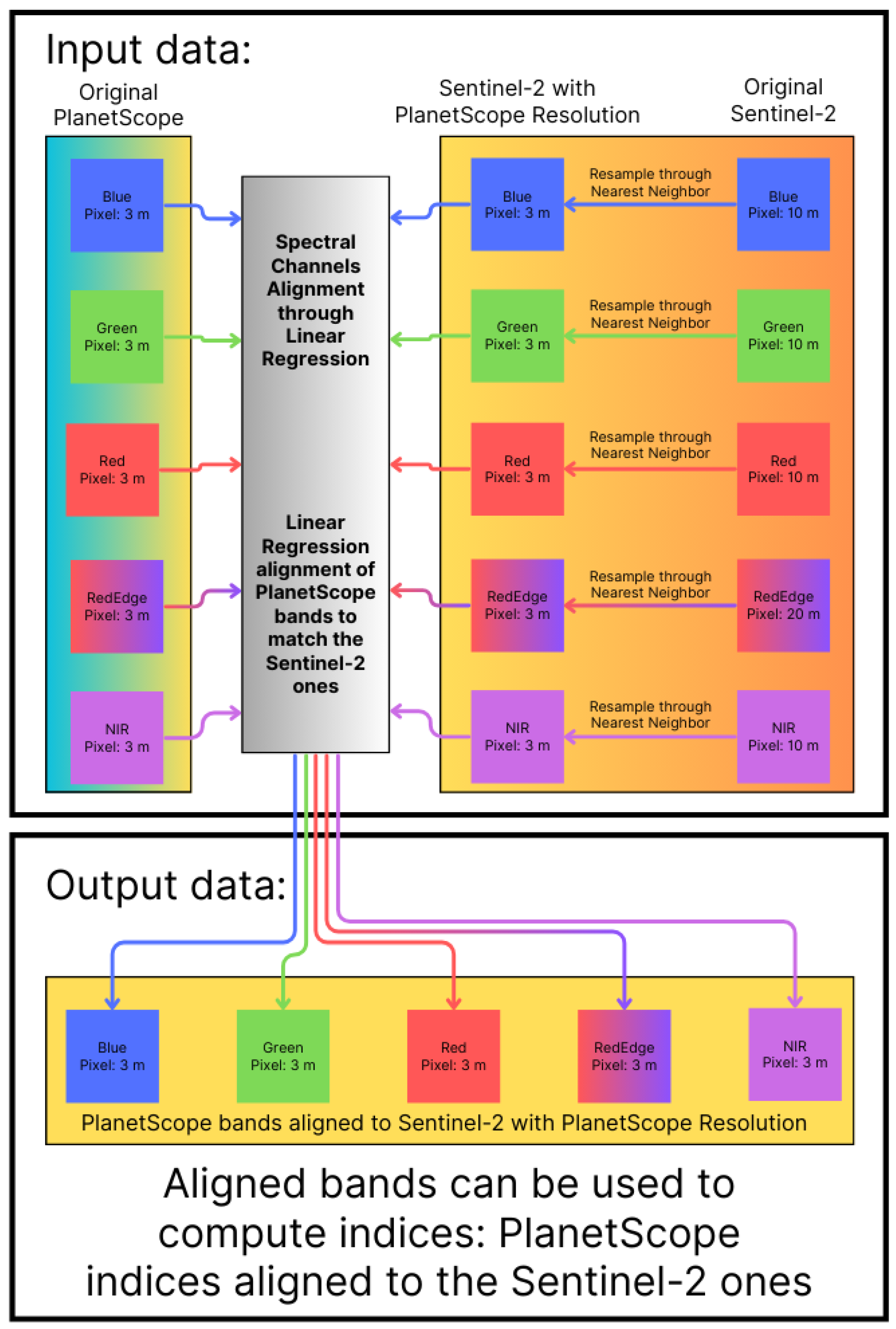
Linear regression [4,45,46,47] is employed to model a linear relationship between a dependent variable that needs prediction and one or more independent variables that serve as predictors. A linear relationship between dependent and independent variables is applied to corresponding pixels of PlanetScope and Sentinel-2. The latter’s NIR, Red, Green, and Blue bands (10 m resolution) and RedEdge band (20 m) are oversampled and aligned [113,114,115,116] to PlanetScope’s 3 m pixel size through the Nearest Neighbor Algorithm [2,116,117]. This implies that the dependent variable changes proportionally with changes in the independent variables. In the context of this study, linear regression was executed using the “fitlm” [47] function in MATLAB R2024b. This function is particularly favored for fitting linear models due to its versatility in model specification, its ability to accommodate categorical predictors, and its comprehensive statistical output. The implementation of “fitlm” [4] necessitates the use of two matrices: one containing the predictor variables and the other containing the variable to be predicted.
The OLS (Ordinary Leath Squares) method was utilized to regress and align the values of individual bands from the PlanetScope sensor to those of the Sentinel-2 sensor. Given the requirement to calibrate PlanetScope responses to those of Sentinel-2, a key objective was to establish the linear equation that could take PlanetScope spectral band values as input and generate output values akin to those of Sentinel-2. Prior studies [11,22] have demonstrated that a buffer zone of 10 m from the borders of rice crops is essential for effectively mitigating edge effects. Consequently, this zone was excluded from linear regression application. In essence, linear regression, as implemented in this study, served as a tool to predict Sentinel-2-like values from PlanetScope data. Linear regression [4,11,47] and the incorporation of a buffer zone to minimize edge effects highlight the methodological rigor applied in this research. An example of linear regression as applied in this paper is reported on the Matlab Website [45] and in a previous paper by the same authors [4].
The selection of the five spectral channels for analysis was meticulously conducted to enable the calculation of indices as highlighted in paragraph 1.4. The selection was examined by comparing the sensors’ central wavelength, full width at half maximum (FWHM), and resolution [7,9,10,14,97,100,103,118]. Alignment was conducted through Sentinel-2 (minimal difference between Sentinel-2A and Sentinel-2B were not considered) and PlanetScope bands reported in Table 2. Figure 5 illustrates the process used to align the bands.
PlanetScope offers Green and Green I channels; only the former is compatible with Sentinel-2. Sentinel-2 provides multiple Red Edge channels, but only the one with a central wavelength at 705 nm is compatible. Following PlanetScope guidelines regarding NIR compatibility, interoperability is radiometrically ensured with Band 8a Narrow NIR in Sentinel-2, which has a resolution of 20 m compared to 10 m of Band 8 Standard NIR. Sentinel-2 [119,120,121,122,123] utilizes two distinct near-infrared (NIR) bands: the broader Band 8 (B8: ~842 nm center, ~115 nm width, 10 m resolution) and the narrower Band 8a (B8a: ~865 nm center, ~21 nm width, 20 m resolution). A key difference is that B8a’s narrow bandwidth is specifically positioned to avoid the atmospheric water vapor absorption feature around 820 nm, which affects the broader B8. This design gives B8a a significant advantage in retrieving surface reflectance measurements that are less sensitive to variations in atmospheric water vapor content, albeit at a coarser 20 m resolution. It is inaccurate to consider B8 and B8a spectrally “nearly identical” due to their substantial differences in central wavelength, bandwidth, and spatial resolution. Furthermore, Sentinel-2 B8a was intentionally designed for spectral consistency with the NIR band of the Landsat 8/9 OLI sensor [124,125,126] (Band 5: ~865 nm center, ~28 nm width, 30 m resolution), facilitating synergistic data use and long-term monitoring efforts between the missions. While B8 might be used for geometric alignment due to its resolution, B8a provides distinct spectral information crucial for specific atmospheric and vegetation studies and cross-sensor comparisons with Landsat 8/9. It is also plausible and often a suitable choice for geometric alignment to use B8 band aerosol correction algorithms (like Sen2Cor [127,128,129]), which typically use other bands (e.g., coastal aerosol, blue, SWIR) to estimate aerosol optical thickness (AOT) and then apply corrections across all bands, including B8 and B8a. The inherent susceptibility might differ slightly due to wavelength, but the corrected products aim to minimize these effects for both. In conclusion, B8a is particularly suitable for applications that demand high radiometric accuracy for detailed vegetation assessment, despite its reduced resolution of 20 m. Conversely, Band B8, which has a resolution of 10 m, is frequently utilized for diverse analytical purposes. This research is endorsed by expert agronomists who employ Band B8, and this study aligns with that selection for comparative analysis.

2.7. Spectral Profiles of Original Bands (Before Resampling)

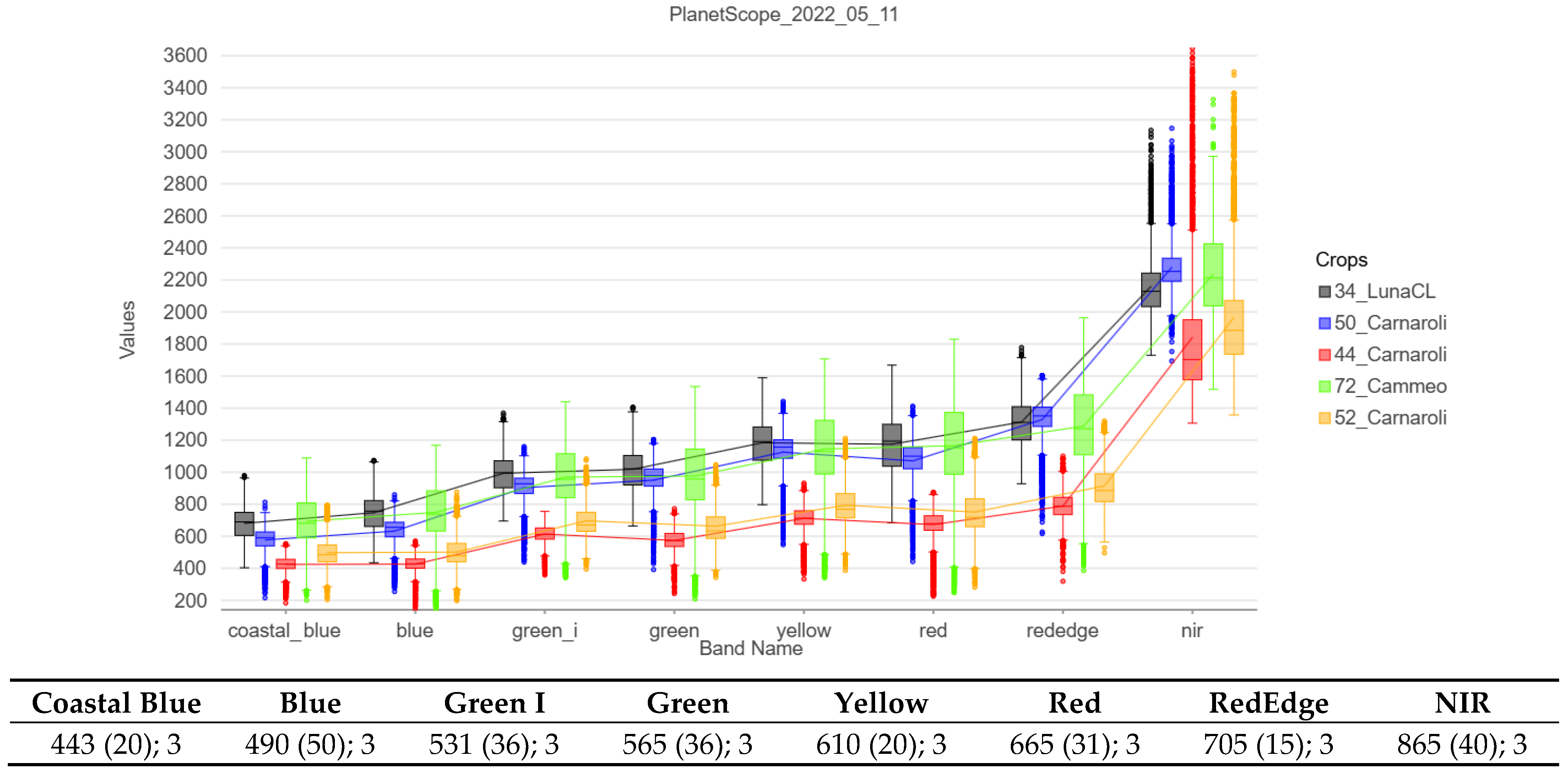
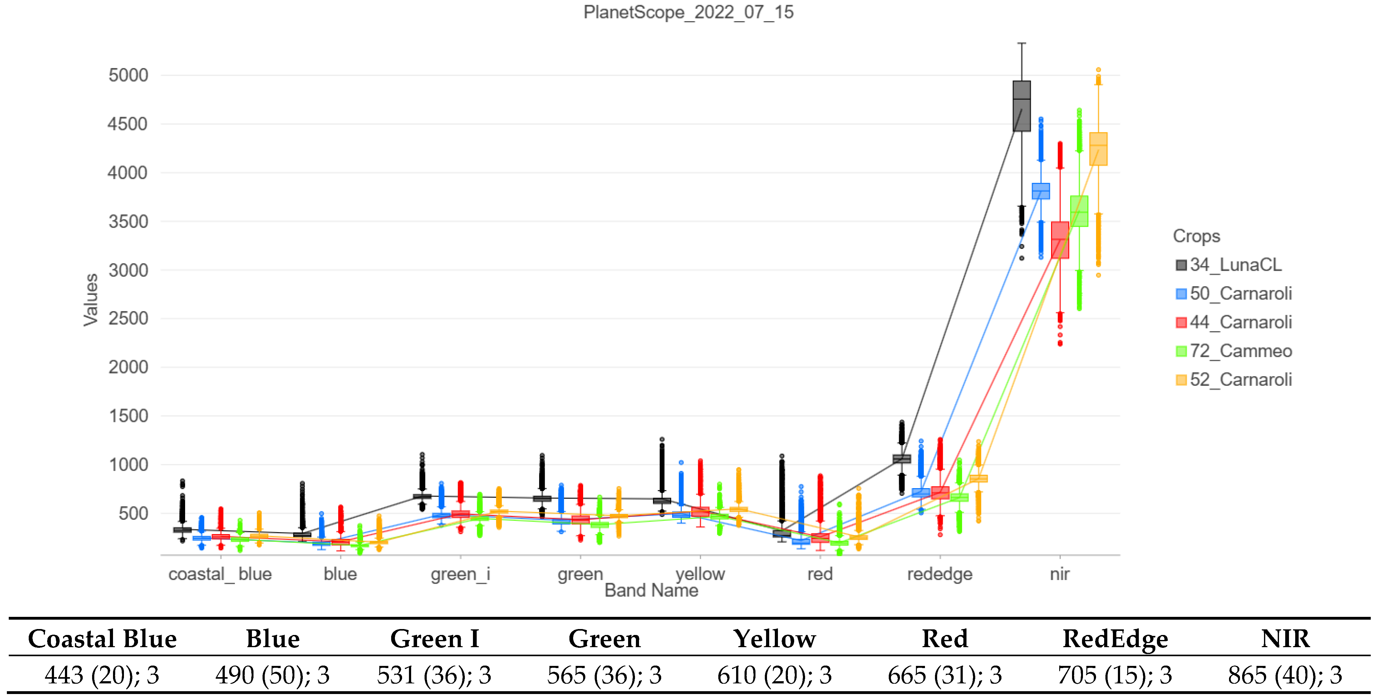
In remote sensing, a spectral profile (or spectral signature) is the quantitative measure of how electromagnetic radiation (EMR) interacts with a material across wavelengths. This graph shows an object’s reflectance, absorption, or emittance based on incident EMR wavelength [28,130]. Different materials like vegetation, soil, water, minerals, and urban surfaces have unique interactions with EMR at various wavelengths, creating distinct spectral profiles for identification. Healthy vegetation reflects strongly in NIR but absorbs red and blue visible light for photosynthesis. Spectral profiles are generated from data measured by remote sensing instruments, which capture the intensity of EMR reflected or emitted from Earth’s surface in specific bands. Each pixel’s digital number or radiance/reflectance value in each band contributes to the spectral profile, plotted with wavelength on the x-axis and radiance or reflectance on the y-axis. An ideal Spectral Response Function (SRF)/spectral profile would be a perfect rectangle, meaning the sensor maintains equal sensitivity across the entire band and zero sensitivity outside it [23]. In practice, SRFs usually appear as bell-shaped curves. Comparing the SRFs of bands in various sensors is crucial for understanding how they average incoming radiation within a band, potentially resulting in variations in measured reflectance values for the same target. Overlapping SRFs between sensors can aid in data integration and comparison. Plotting the SRFs of corresponding bands from different sensors enables a visual and quantitative assessment of their overlap and shape, which helps predict how similar or different the measured values will be for spectrally varying targets. Five fields far from each other, to limit spatial autocorrelation [131,132], were chosen to be compared through their spectral profiles before analysis to compare their scaling: three Carnaroli Rice, one Luna CL, and one Cammeo. Figure 6 shows where these crops are placed through the rice farm and Figure 7 shows the electromagnetic spectrum [133] with frequencies/wavelength/color association. Figure 8 and Figure 9 illustrate the spectral profiles for the 11 May 2022 pair of images while Figure 9 and Figure 10 illustrate the spectral profiles for 15 July 2022. Certain varieties exhibit similar spectral profiles, such as the Carnaroli crops during both the growing stage and fertilization period. Additionally, Luna CL and Cammeo display comparable behaviors, although there are slight differences between them. When comparing these graphs for the same crops, it is clear that each sensor responds differently to similar frequencies (which correspond to the bands). A statistical introduction is required to deepen the analysis.
Spectral profiles are presented in this research using boxes and mean lines and are centered over EMR Figure 7 frequencies. A box and whiskers plot summarizes the distribution of data through its quartiles: it is constructed using five key statistical values: the minimum value, the first quartile (Q1), the median (Q2), the third quartile (Q3), and the maximum value [134,135,136,137].
The rectangular box represents the interquartile range (IQR), which includes the middle 50 percent of the data values. The bottom edge of the box corresponds to the first quartile (the 25th percentile), indicating that 25% of the pixel values fall below this point. The top edge of the box represents the third quartile (the 75th percentile), meaning that 75% of the pixel values are below this point. A line passing inside the box indicates the median (the 50th percentile), which is the middle value of the dataset. Vertical lines, known as whiskers, extend from the top and bottom edges of the box to a length 1.5 times the interquartile range (IQR). Data points beyond these whiskers are considered outliers. The interquartile range (IQR), represented by the height of the box in the box plot, is a measure of the spectral variability within the selected area of interest for a particular band.
A large IQR suggests dispersion of pixel values, indicating spectral heterogeneity. This might occur in areas where ground cover is not uniform, such as pixels on the boundary between different land cover types or an area containing mixed materials. Conversely, a smaller IQR indicates clustering of pixel values around the median, suggesting a spectrally homogeneous area.
By examining the shape and size of the boxes across different spectral bands in a spectral profile, it is possible to understand how the distribution of pixel values changes with the wavelength. For example, a particular band might exhibit a large IQR and a high median value, indicating variability in reflectance but a tendency towards higher reflectance in that part of the electromagnetic spectrum. Comparing these box plots across all bands provides information about the spectral characteristics of the chosen area of interest.
Mean line plot displays the average spectral reflectance for a selected area of interest across the different bands of the image. It calculates the mean pixel value for each band within the defined area and connects these mean values with a line, creating a graphical representation of the overall trend in spectral response across the electromagnetic spectrum for the chosen feature or region. Mean lines provide a view of the spectral signature, highlighting the average reflectance values for each band and allowing for an assessment of the general spectral characteristics of the area.
Outliers refer to pixel values for a specific band within a selected area of interest that lie outside the normal distribution of values for that band. These values can provide further insight into the data and might indicate mixed pixels, shadows, or unique surface materials that are spectrally distinct from the surrounding area.
Outliers can be attributed to several factors. One cause is the occurrence of mixed pixels, especially in imagery with coarser spatial resolution. A mixed pixel covers an area containing more than one type of land cover or material, resulting in a combination of spectral signatures that deviate from purer pixels representing a single land cover type. Outliers can also represent rare or unusual surface conditions, noise, or errors in the data that need consideration during analysis steps.
The data indicates that in May, there is a significant number of outliers in the higher values for RedEdge and NIR, and a substantial number of outliers in the lower values for Blue, Green, and Red. Conversely, in July, a large number of outliers are observed in the lower values for RedEdge and NIR, while Blue, Green, and Red exhibit a considerable number of outliers in the higher values. Additionally, the number of outliers in July is smaller compared to May: this may be a factor contributing to the higher RMSE and MAER observed in previous research during May [2,3,4,11,21,22]. Band data are available from the producers websites [7,12]. Comparing spectral profile of images acquired the same day it is possible to verify the different scaling for the same frequencies: 11/05/2022 (Figure 8 Sentinel-2 and 9 PlanetScope) and 15/07/2022 (Figure 10 Sentinel-2 and Figure 11 PlanetScope).

3. Results

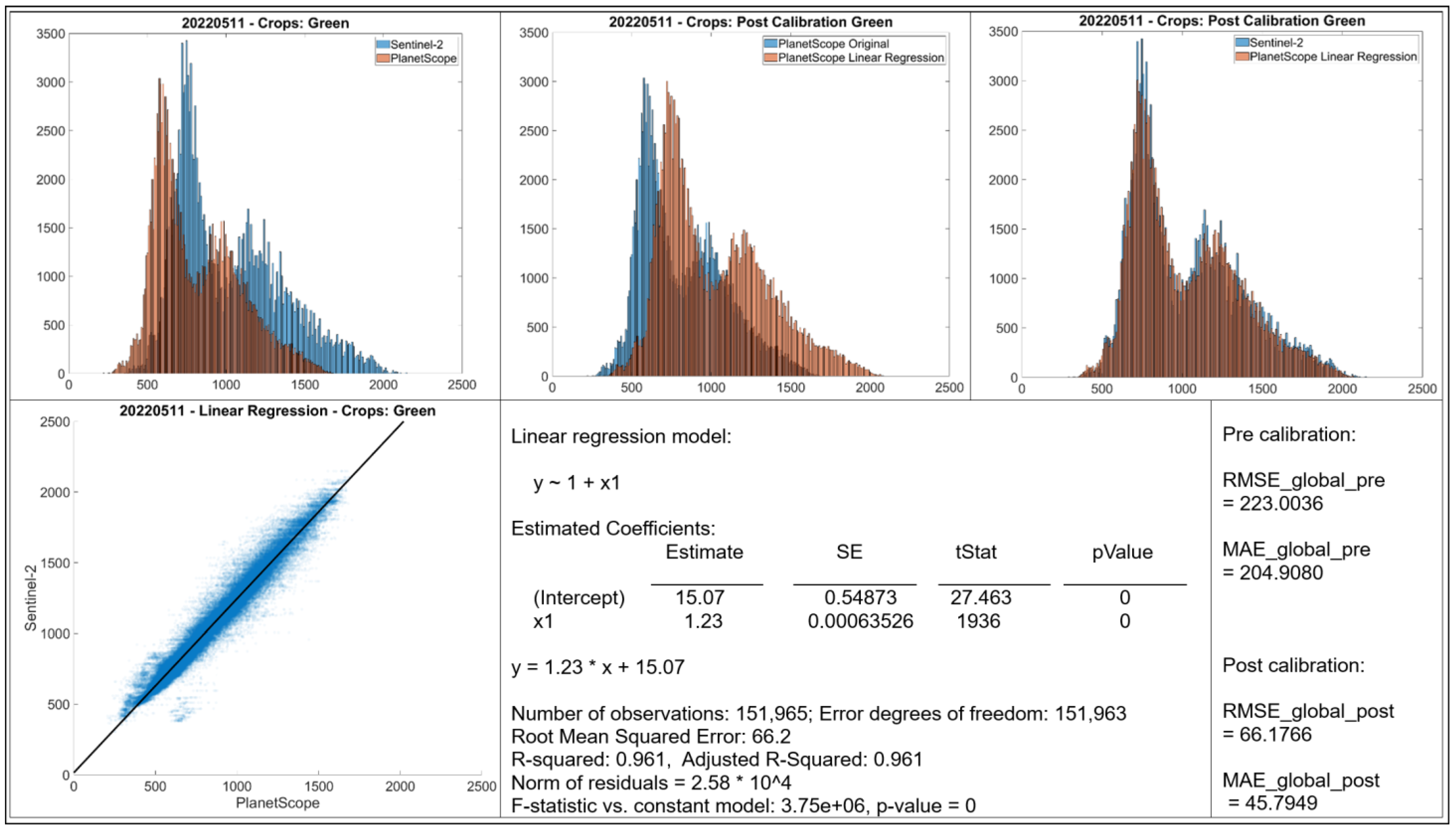
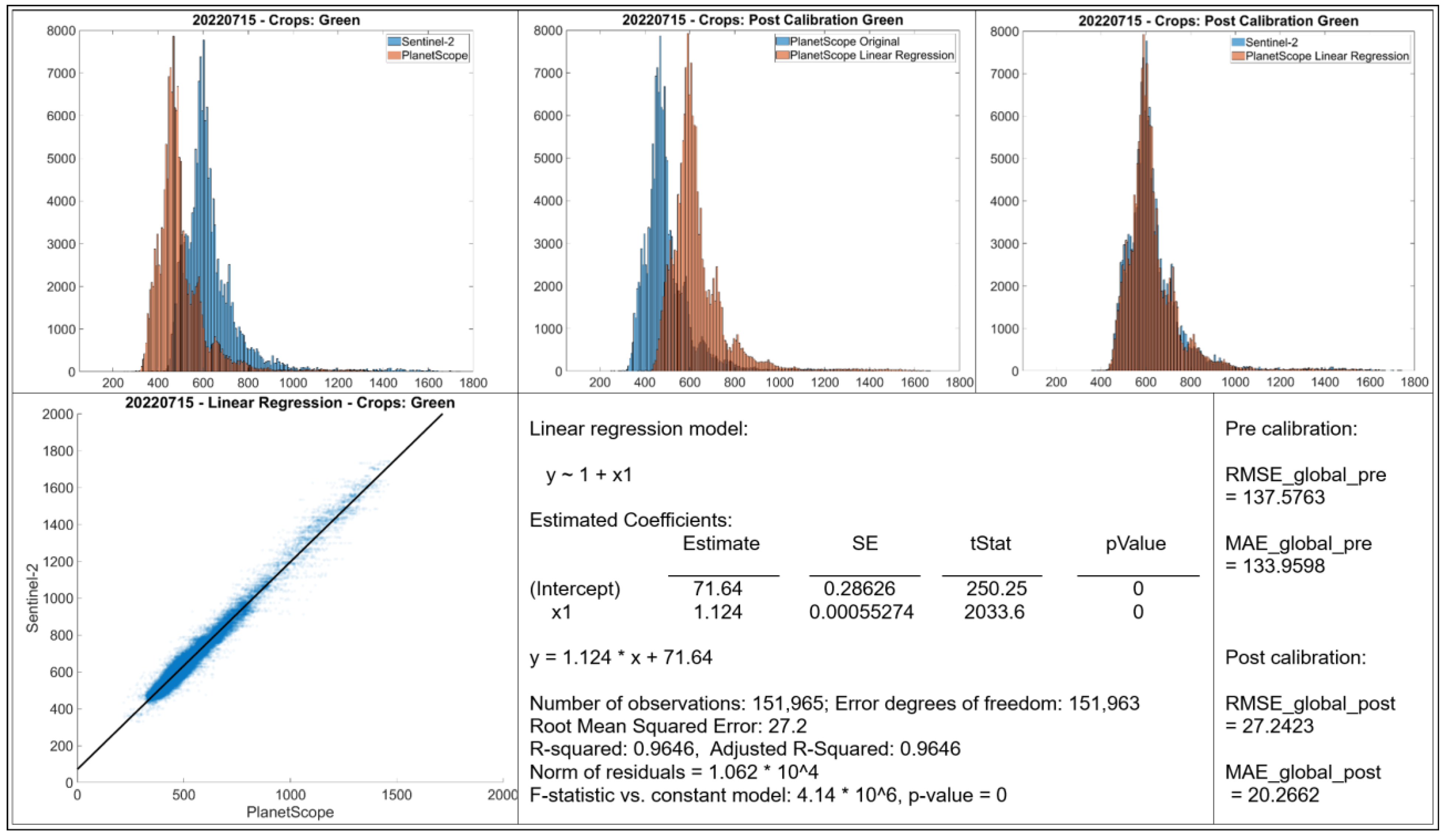
Summary of Presented Data for each calibration through Linear Regression:
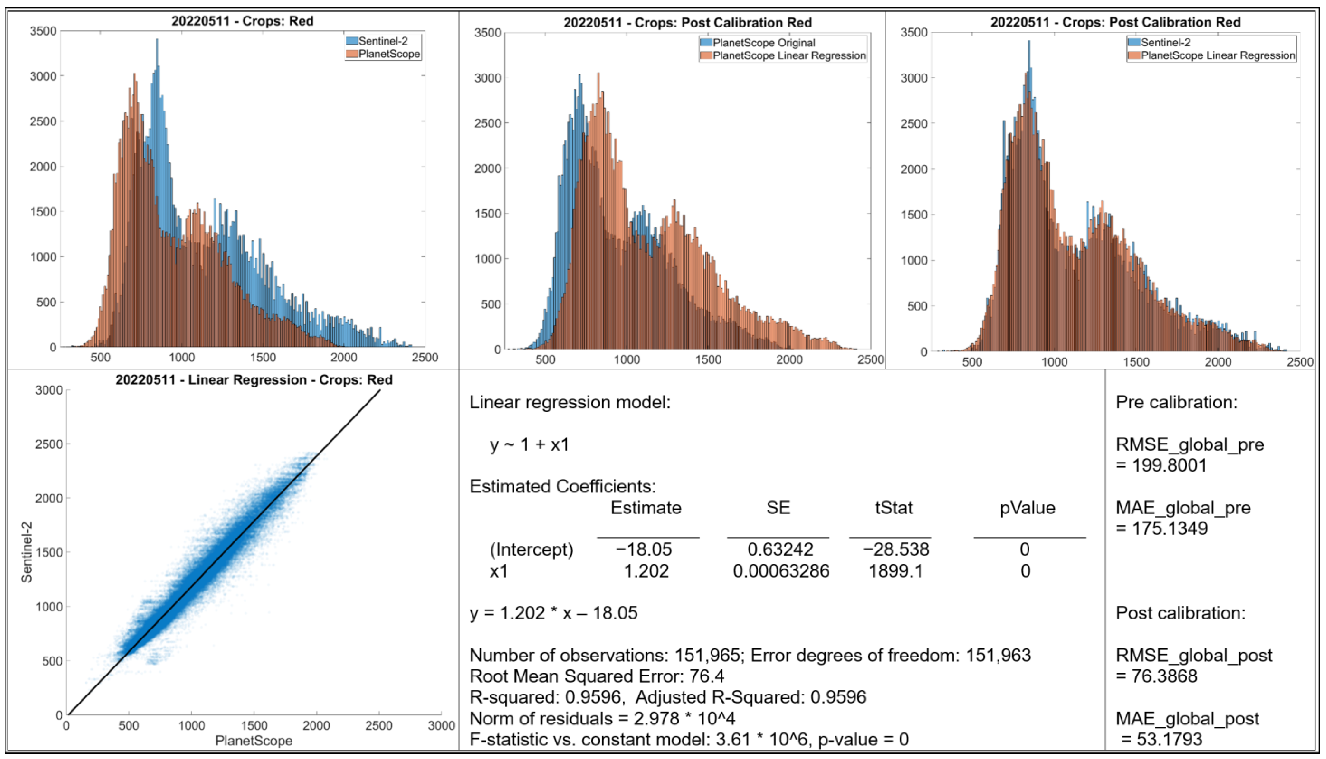
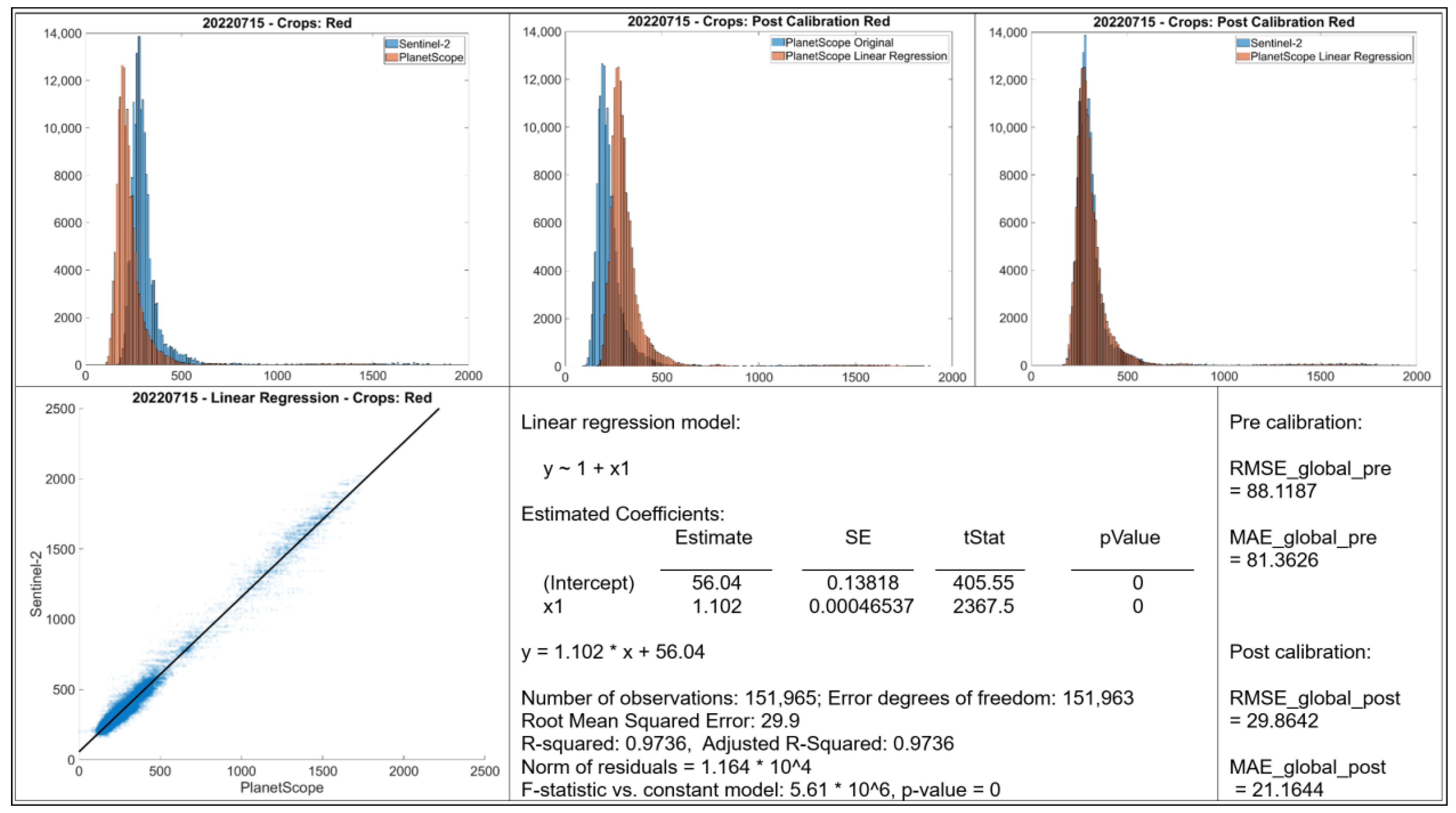
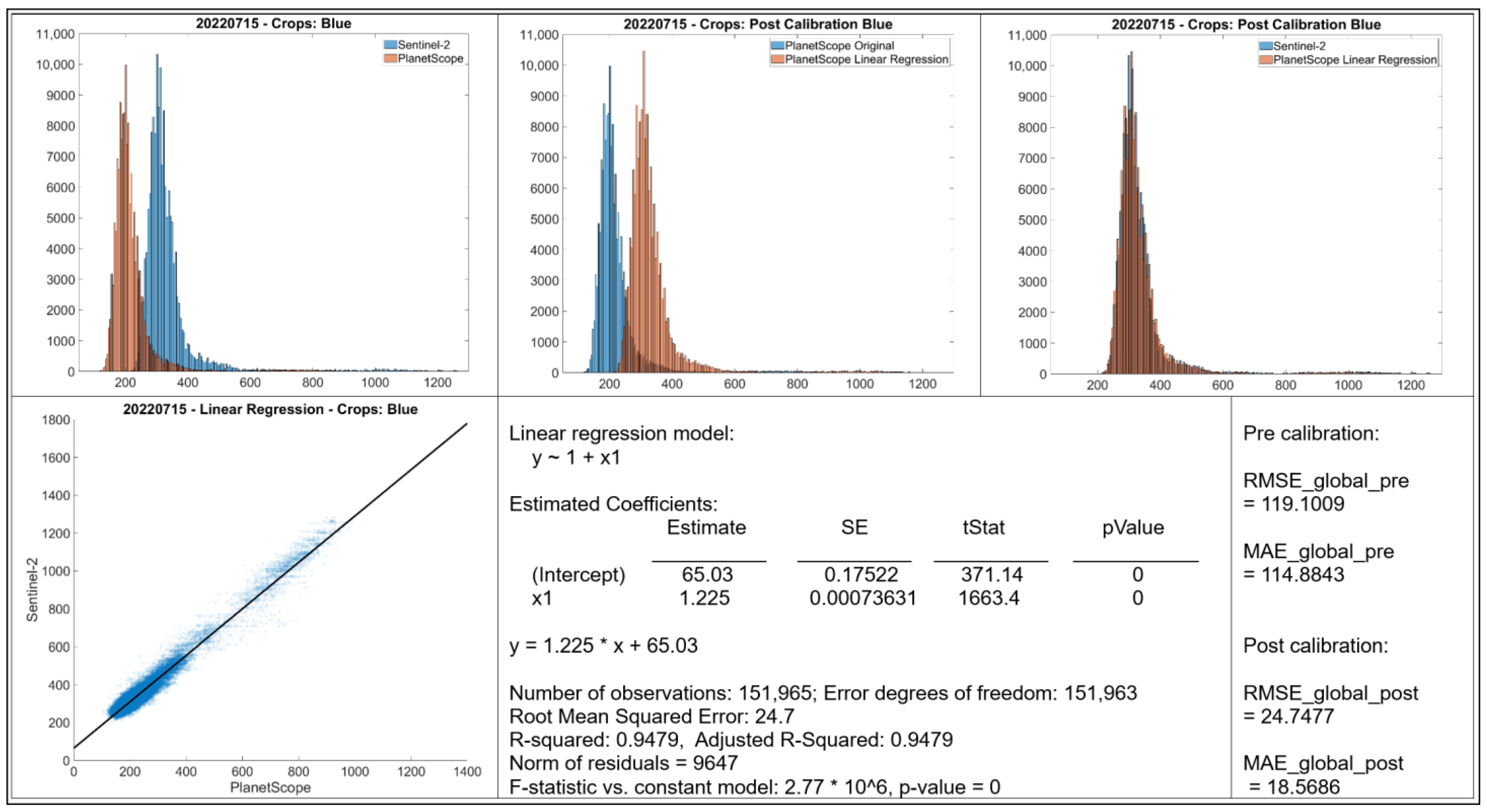
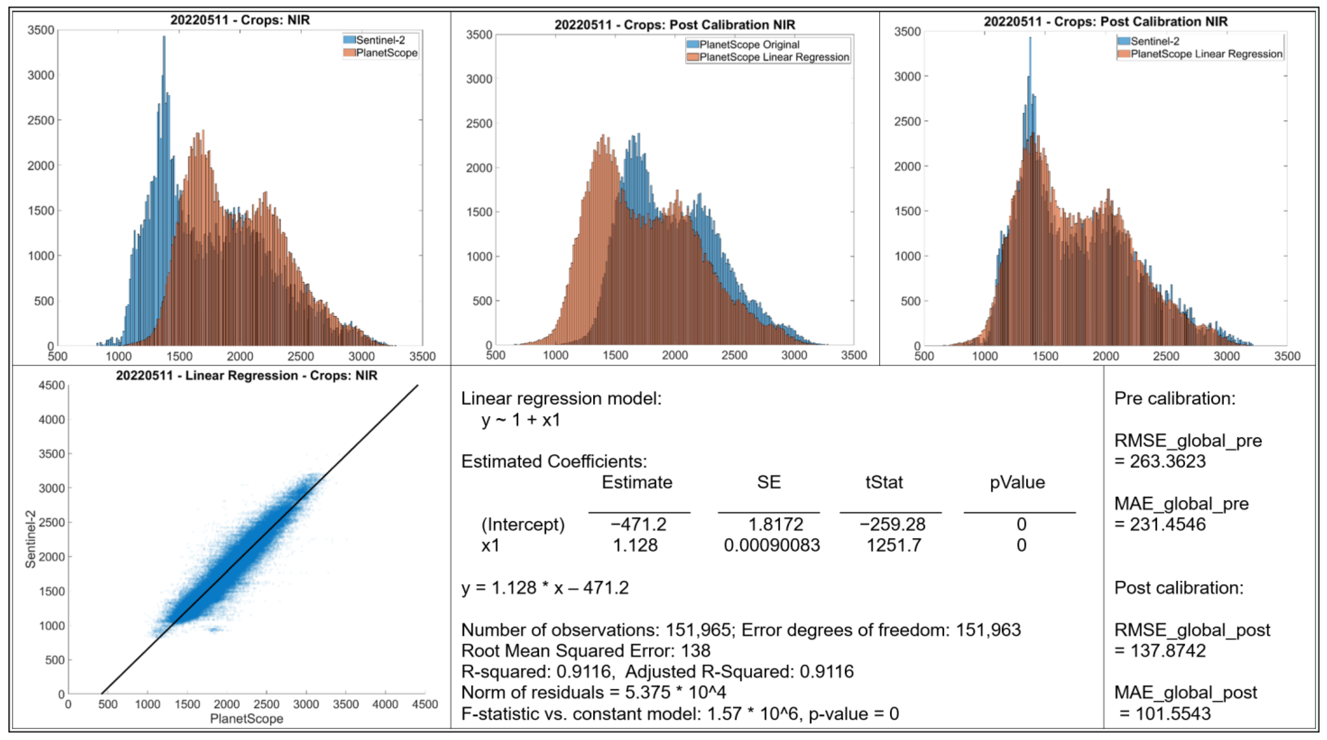
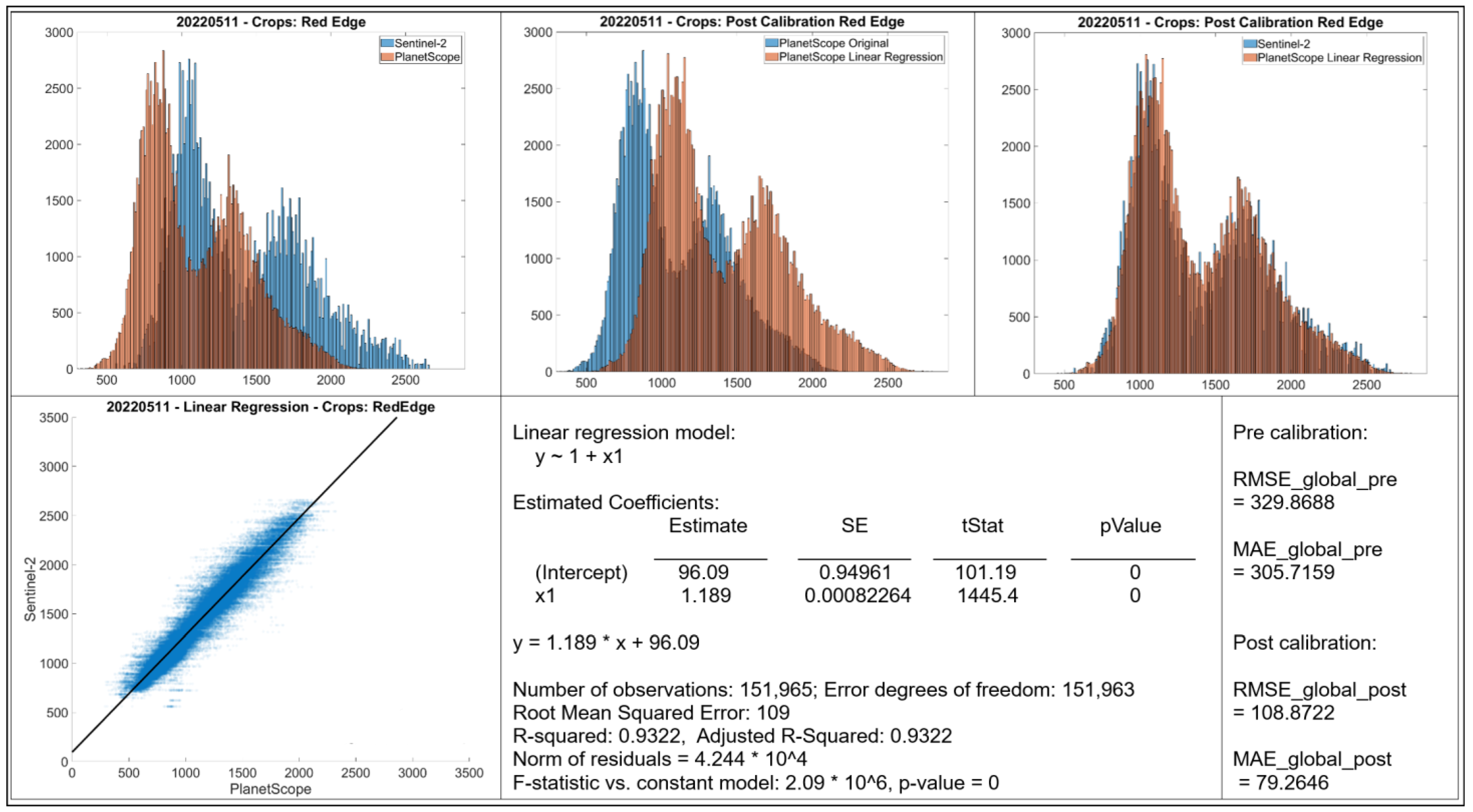
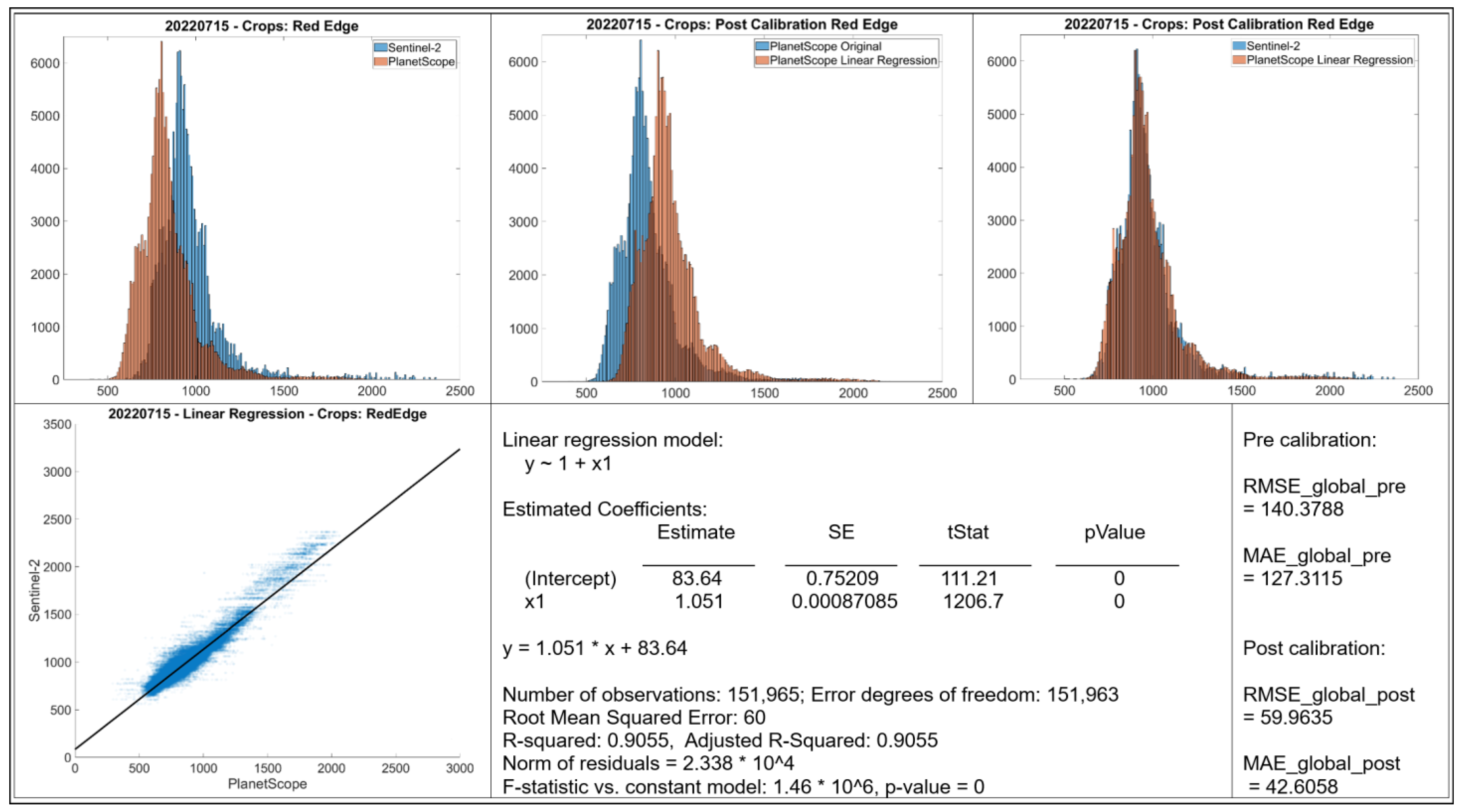
  • Histograms: The top row displays histograms of the band values. The leftmost plot displays the original distributions for Sentinel-2 and PlanetScope, showing differences in the range and frequency distribution of values between the two sensors. The middle and rightmost plots present the distributions after applying linear regression-based calibration to the PlanetScope data. In each case, the calibrated PlanetScope distribution is more closely aligned with the Sentinel distribution compared to the original data.
  • Scatter Plot: The bottom left plot presents a scatter plot illustrating individual data points of Sentinel-2 band values against original PlanetScope band values. Each case demonstrates a strong linear relationship, with data points clustering along a diagonal trajectory, indicating that a linear model is an appropriate choice for calibration.
  • Linear Regression Model: Information about the fitted linear regression model is given, where Y represents the predicted Sentinel-2 value and X represents the original PlanetScope value.
  • The RMSE and MAE values before and after linear regression are shown.
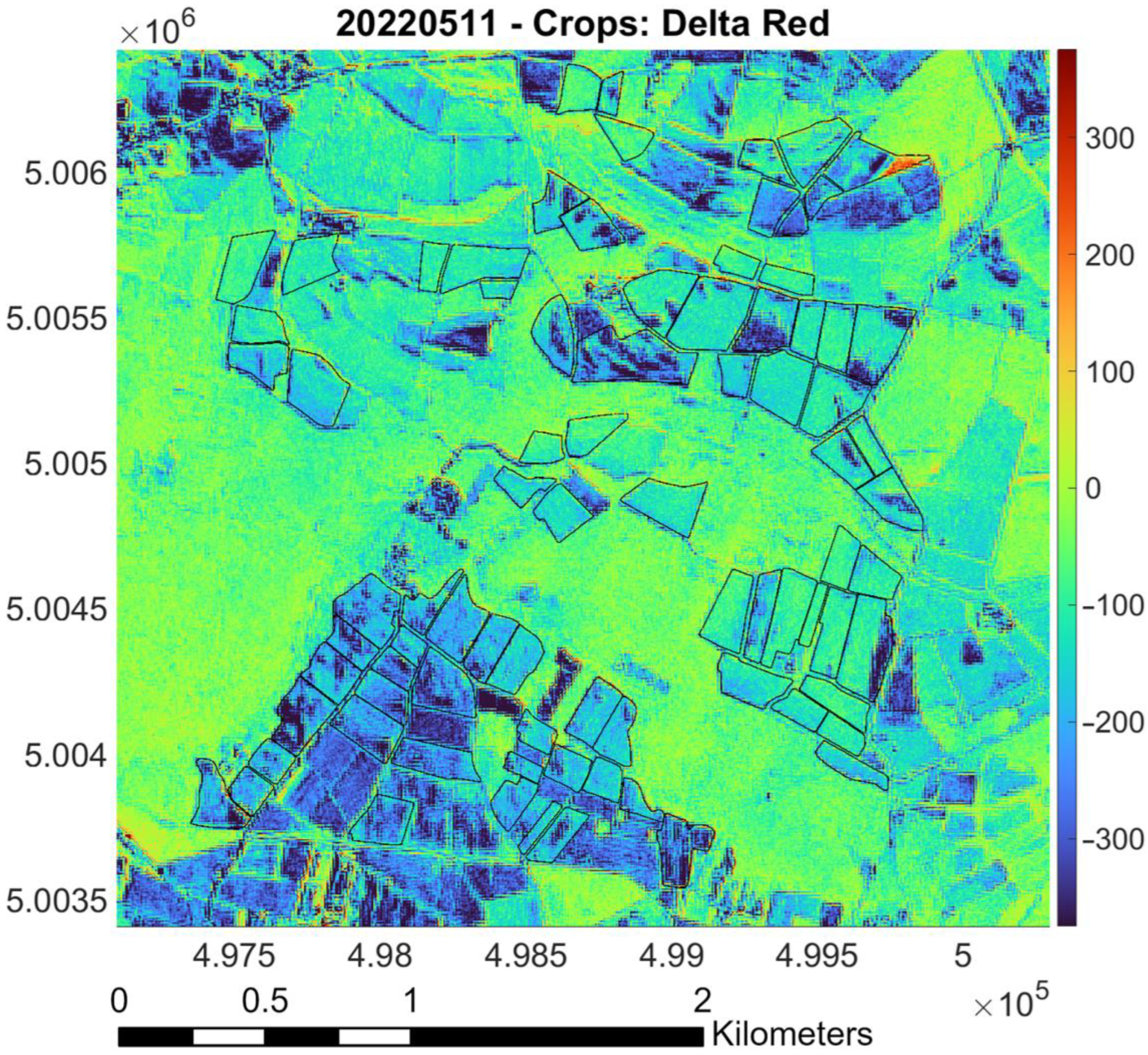
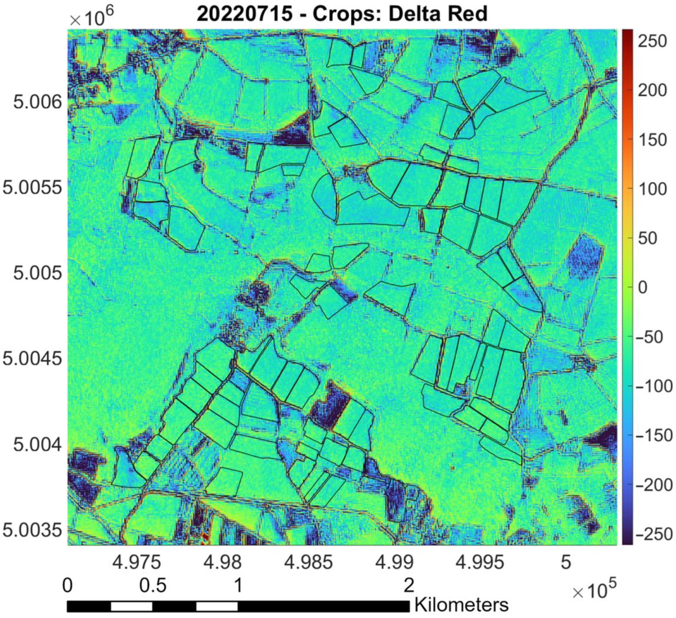
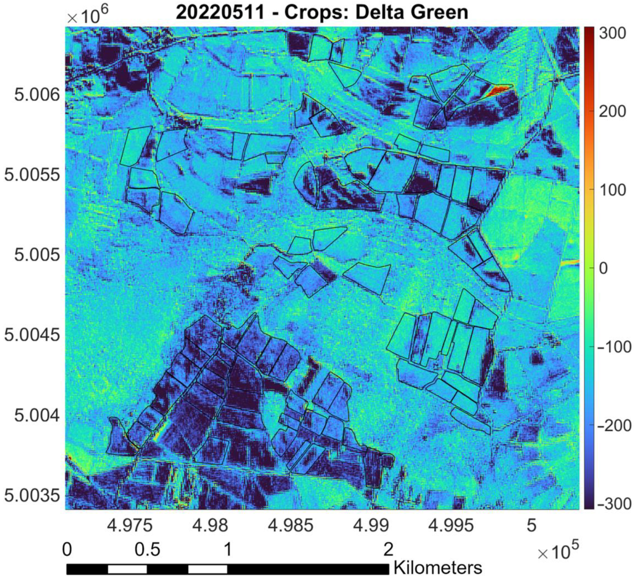
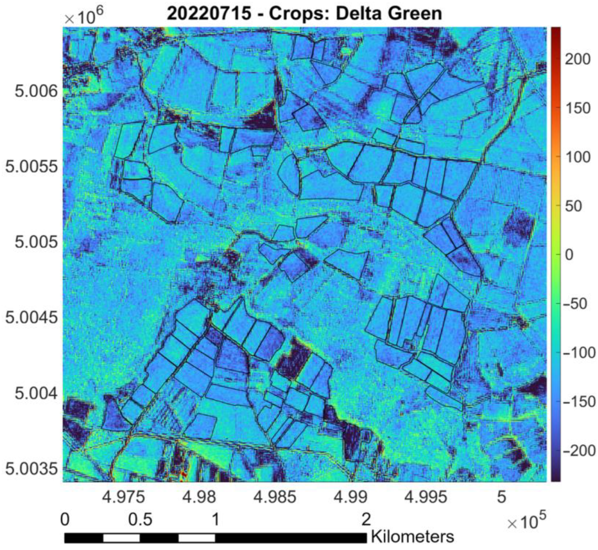
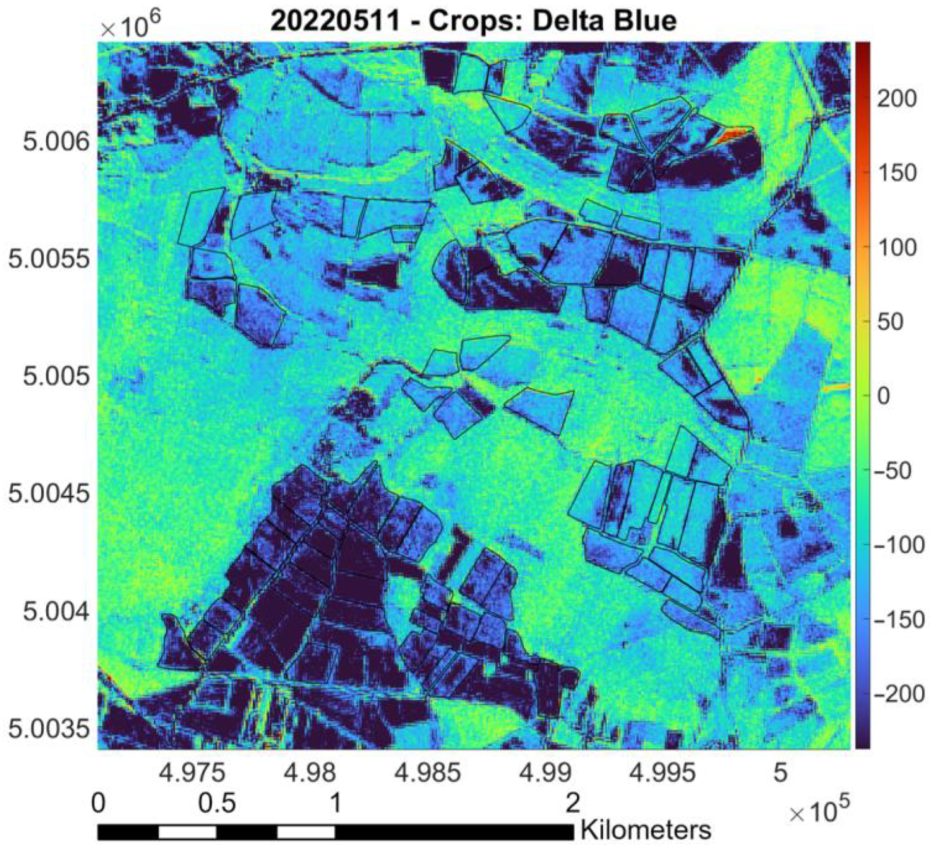
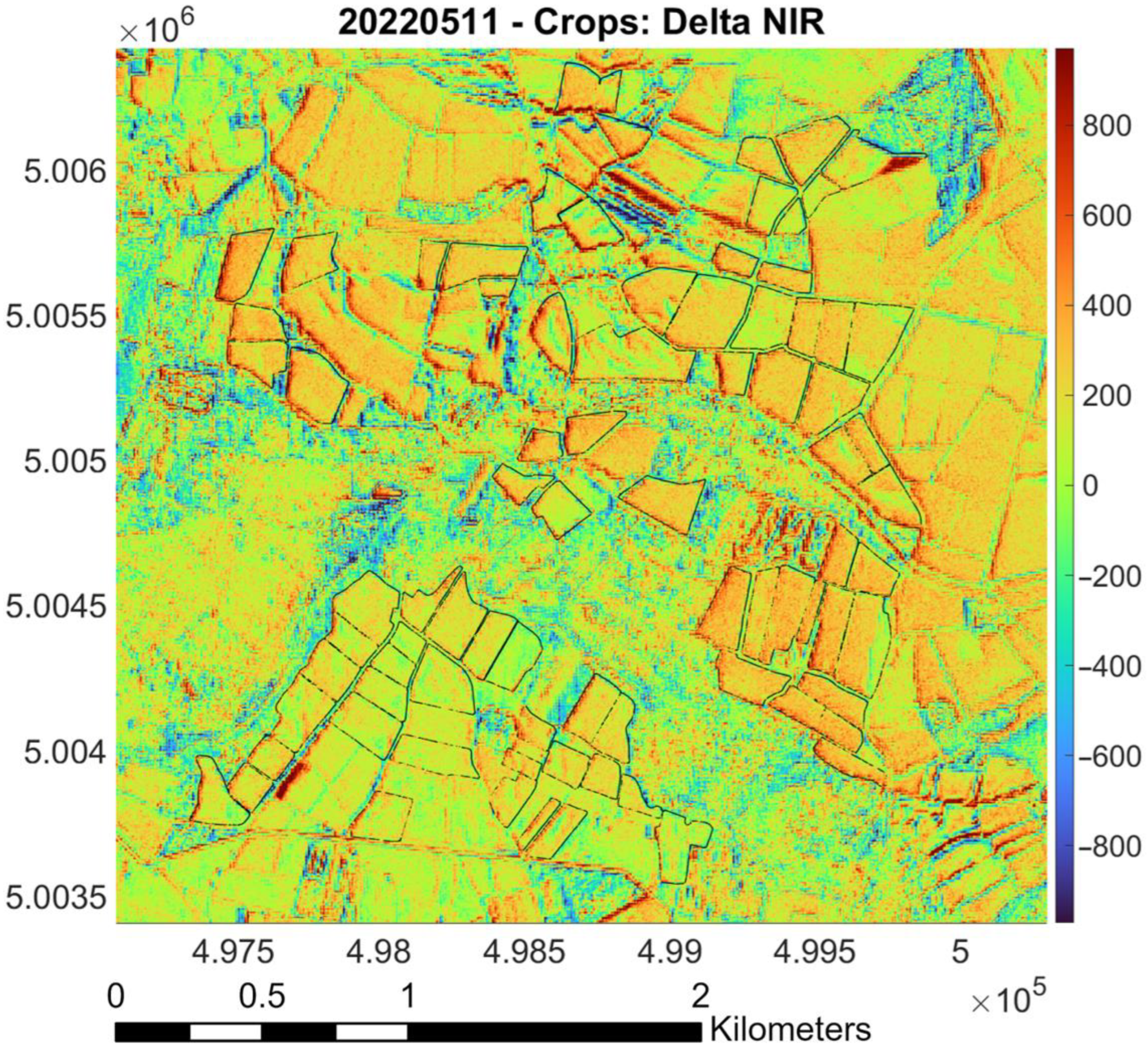
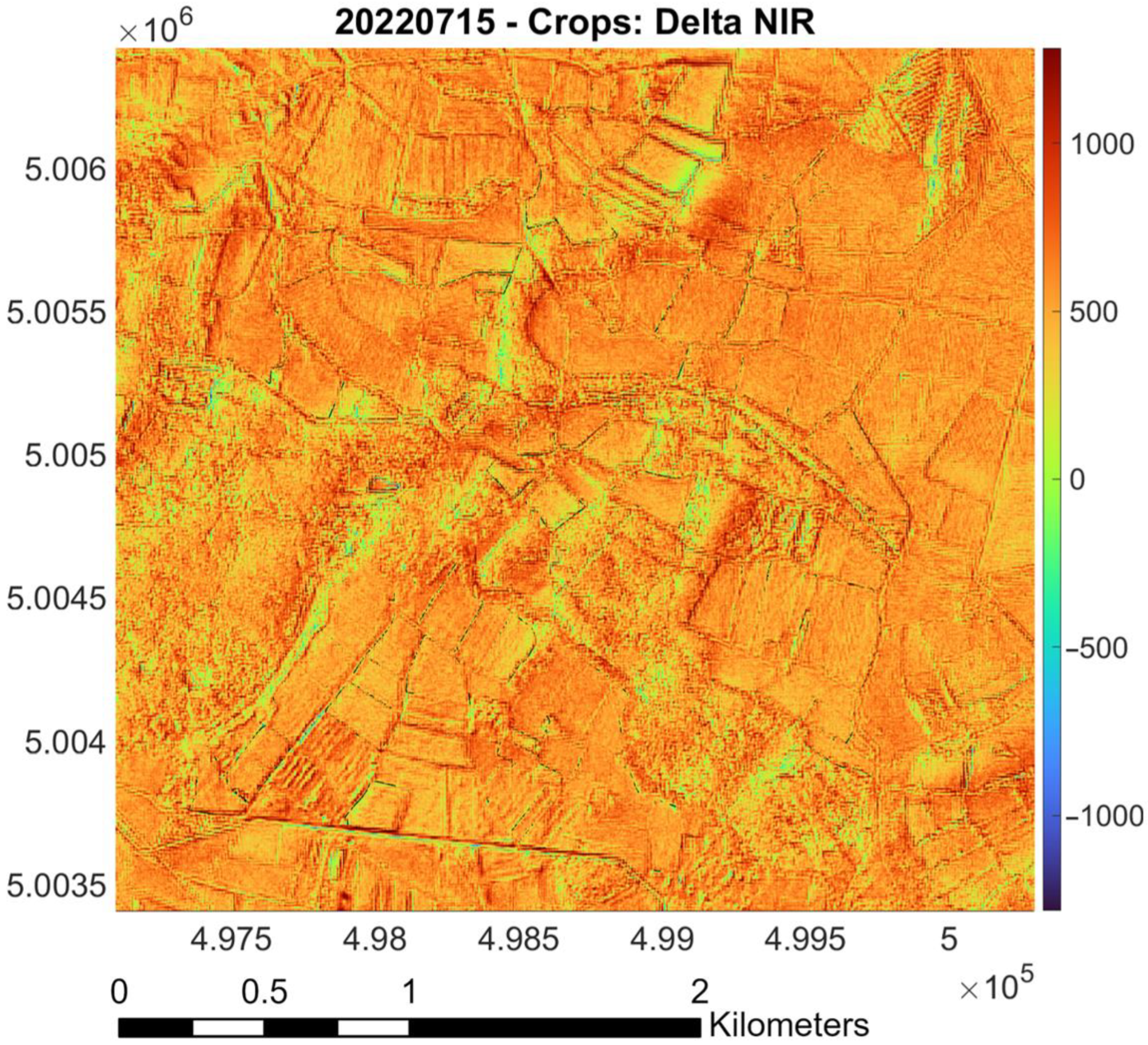
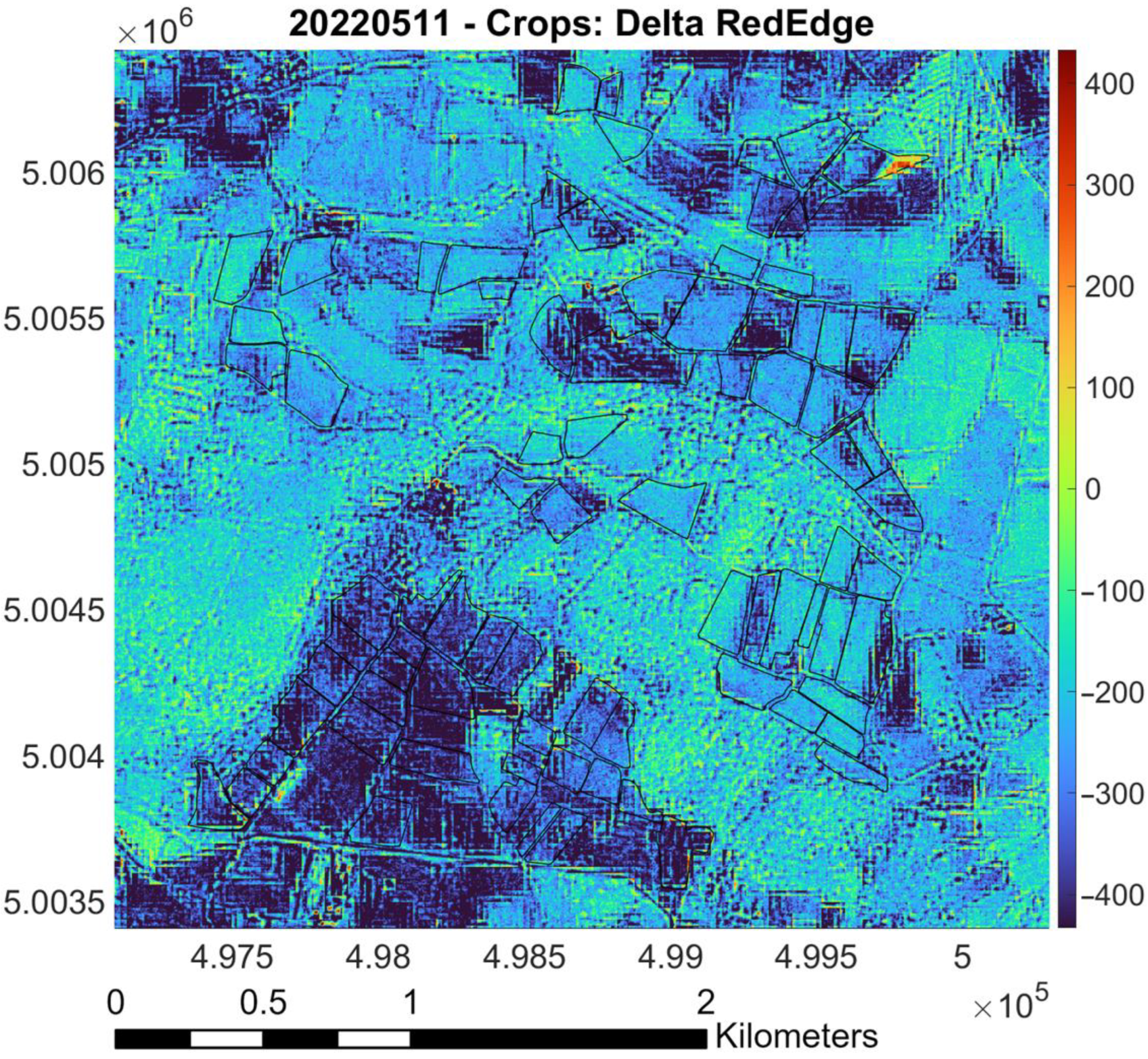
  • Raster difference between PlanetScope and Sentinel-2 (as reference): Red pixels indicate areas where PlanetScope values are significantly higher than Sentinel-2 values; blue pixels represent regions where Sentinel-2 values surpass those of PlanetScope. Green and yellow markers denote areas with similar values, based on the magnitude of the difference. The color bar indicates the values of the difference between the surface reflectances measured by the two sensors. Black lines outline “Riserva San Massimo” rice crop boundaries.
Each scatter plot clearly illustrates a strong linear correlation between the two datasets, justifying the selection of a linear model for calibration. The statistical results of the linear regression model confirm this strong relationship. The extremely high R-squared value indicates that the linear models effectively capture the relationship between the two sensors’ band measurements for this specific date and crop type. The highly significant p-values for both the intercept and slope coefficients, as well as the overall model F-statistic, provide strong statistical evidence that the fitted linear relationship is not due to random chance. The F-statistic compares the amount of variance explained by the regression model to the amount of variance that remains unexplained (the residual variance). A larger F-statistic indicates that the variance explained by the model is considerably greater than the unexplained variance, lending support to the rejection of the null hypothesis. The RMSE of the model represents the residual error after fitting the linear relationship. Crucially, the comparison of pre- and post-calibration error metrics provides quantitative evidence of the calibration’s effectiveness. The significant reduction in both RMSE and MAE demonstrates that the linear calibration substantially reduced the systematic differences between the Sentinel-2 and PlanetScope band values. Based on the provided data, the linear regression calibration appears successful in reducing the discrepancy between the Sentinel-2 and PlanetScope bands. The oversampling of data from Sentinel-2 impacted the results. PlanetScope data were downsampled to a 10 m resolution during the research to understand this effect, producing comparable outcomes. After optimally aligning the PlanetScope images using these techniques, it is possible to generate prescription maps within acceptable limits. The methodology is scientifically evaluated, employing standard statistical techniques to quantify the relationship and assess the improvement. By examining the spectral profiles in Figure 8, Figure 9, Figure 10 and Figure 11 and comparing them with the histogram prior to linear regression, it becomes evident that the corresponding bands exhibit varied responses to the same input. Therefore, alignment is essential and can lead to improved calibration.

3.1. Calibration for Red Band (May and July)

Calibration effectively reduced discrepancies between the original PlanetScope Red band data and the Sentinel reference data for both analyzed dates comparing May acquisitions (Figure 12 and Figure 13) with July acquisitions (Figure 14 and Figure 15). The calibration significantly lowered RMSE and MAE values. Differences in the derived linear models and post-calibration performance metrics between the two dates indicate that optimal calibration parameters may vary over time, suggesting that temporal variations should be considered in operational calibration procedures. Difference rasters offer key information about the starting conditions and effectively pinpoint locations with considerable change (comparing Figure 13 and Figure 15). High R-squared values confirm the strong linear relationship between the datasets, supporting the use of a linear model for this application.
Most of the differences are observed over crops because, in areas with woodlands, the scale appears quite similar between the two sensors in the red channel. The histograms differ significantly between the two periods. In July, vegetation is dense, while in May, it is sparse, and during the rice farming season, the conditions vary: sometimes the crops are wet, sometimes they are not, and at times there is barren land. The variability assessed by the agronomist is critical for understanding as it represents the most challenging period for calibration assessment. The red pixel values of Sentinel-2 consistently exceed those of PlanetScope. Most of the crops exhibit a good alignment even before the LR.

3.2. Calibration for Green Band (May and July)

Even the Green calibrations, similar to the Red band, exhibit significant reductions in RMSE and MAE values post-calibration, affirming that the linear regression model successfully minimizes discrepancies comparing May acquisitions (see Figure 16 and Figure 17) with July acquisitions (see Figure 18 and Figure 19). High R-squared values in both cases indicate a strong linear relationship between the datasets. Temporal variations observed in both calibrations suggest the necessity of considering time-specific calibration parameters for optimal performance: an examination of the Difference Rasters (Figure 17 and Figure 19) reveals this observable evidence especially over crops.
Certain southern crops exhibit significantly higher Sentinel-2 values compared to the corresponding PlanetScope values; this phenomenon is partially observable in the red channel as well. There are no notable differences between these crops, except for their placement at different elevations, as illustrated in Figure 32 (discussion paragraph, considered as a future field of research).

3.3. Calibration for Blue Band (May and July)

The calibration minimized discrepancies between the original PlanetScope Blue band data and the Sentinel reference data for both dates, with significant reductions in RMSE and MAE comparing May acquisitions (Figure 20 and Figure 21) with July acquisitions (Figure 22 and Figure 23). Differences in the linear models suggest the need for periodic reassessment of calibration parameters due to temporal fluctuations: even in this case difference rasters are evidence of this behavior (compare Figure 21 and Figure 23). High R-squared values confirm a strong linear correlation, validating the use of a linear model for calibration.
The same southern crops that exhibit higher Sentinel-2 values compared to the corresponding PlanetScope values in the red and green channels demonstrate similar behavior in the blue channel.

3.4. Calibration for NIR Band (May and July)

Calibration results for the NIR band acquisitions in May (Figure 24 and Figure 25) and July (Figure 26 and Figure 27) show improved data accuracy post-calibration, with high R-squared values indicating strong correlations between datasets (see Figure 24 and Figure 26). The differences in coefficients suggest that calibration parameters need periodic adjustment to maintain accuracy as even Difference rasters demonstrate clearly comparing Figure 25 and Figure 27.
The near-infrared (NIR) band displays different characteristics compared to the visible bands of Red, Green, and Blue. For NIR, PlanetScope values are generally higher than those of Sentinel-2. For the July data, all pixel values in Sentinel-2 are higher than those in PlanetScope (thanks to the difference raster comparison in Figure 25 and Figure 27).
The near-infrared (NIR) bands exhibit the most significant differences, consistently showing higher values in PlanetScope compared to Sentinel-2. This discrepancy may be attributed to the difference between Sentinel bands 8 and 8a. However, this linear regression indicates that it is possible to address this issue, as the dependency is clearly linear.

3.5. Calibration for RedEdge Band (May and July)

The calibration for the RedEdge band shows better error reduction and consistency compared to the NIR band, especially between the analyzed dates: May acquisitions (Figure 28 and Figure 29) and July acquisitions (Figure 30 and Figure 31). Adjusting calibration parameters based on seasonal variations is essential for accurate remote sensing and even in this case difference rasters (Figure 29 and Figure 31) highlight areas of significant variability. The RedEdge band (as for RGB bands) originally has higher Sentinel-2 values, while the NIR band has higher original PlanetScope values.
RedEdge behaves similarly to Red, Green, and Blue, with PlanetScope pixel values exceeding those of Sentinel-2.

3.6. Differences Between Histograms

The linear regression models for the bands show variations between the two dates, with different intercept and slope values. This reinforces the observation regarding temporal variability in the sensor relationship seen also in previous research [2,4,11]. RMSE and MAE values are consistently reduced: the post-calibration RMSE and MAE values for the calibration on 15 July 2022 are lower than those for the calibration on 11 May 2022. This indicates that the calibration performed for July images was more effective. Additionally, the R-squared values are high for both dates, suggesting that the linear model is well suited for describing the relationship between the original and reference band data. Discrepancies in the scaling of bands between the two sensors were identified through the comparison of their spectral profiles, the difference rasters, and their linear regression, leading to inconsistencies in indices observed during prior research [2,4]. These differences arise due to variations in the way each band’s data are represented and measured. To mitigate this problem, linear regression can be employed as a preprocessing technique to align the bands. This method was implemented through Matlab 2024 b [45,46,47,138] in the current research. This alignment ensures that the data across all bands are on a consistent scale. It is important to note that this technique is most effective when applied to bands that are considered compatible by their producers, as compatibility indicates that the bands share similar characteristics and are suitable for comparison. Shifts are observed across all bands, but they do not have the same consistency for each band: Red, Green, Blue, and RedEdge have Sentinel-2 values higher than PlanetScope, while the NIR band shows Sentinel-2 values lower than PlanetScope before linear regression. These shifts are unevenly distributed across the bands and result in ineffective compensation across indices. Consequently, applying linear regression directly to the index yields inefficient results [4]. Calibrating directly indices necessitates several improvements in calibration and employs various techniques such as histogram shifting and histogram matching [4]. In contrast, aligning bands requires only linear regression. It is crucial to assess these results to determine the most appropriate methodology for each specific case [4].

4. Discussion

The research compared five bands from Sentinel-2 and PlanetScope over the “Riserva San Massimo” rice farm, analyzing their characteristics and spectral profiles across crops.
The data reveal that in May, the RedEdge and NIR bands have more high-value outliers, while the Blue, Green, and Red bands have more low-value outliers. Conversely, in July, the RedEdge and NIR bands show more low-value outliers, and the Blue, Green, and Red bands have more high-value outliers. Additionally, the number of outliers in July is smaller compared to May. This highlights the effectiveness of using linear regression (OLS) to align the Blue, Red, Green, RedEdge, and NIR bands. Linear regression models the relationship between two variables by fitting a linear equation to the observed data. Therefore, it is crucial that pixel sizes are uniform and spatially aligned. Sentinel-2 offers Blue, Green, Red, and near-infrared (NIR) bands at a spatial resolution of 10 m, as well as RedEdge at 20 m. In contrast, PlanetScope provides all its bands at a spatial resolution of 3 m. Pixels were aligned ultimately using Nearest Neighbor Resampling [116,117] with posting vectors through Matlab [113,114] to limit spatial correlation [131,132]. Throughout the research, various approaches and resampling algorithms [113,114,115,116,139,140,141] were utilized (linear, cubic, spline, makima [142], …), yielding comparable outcomes. Consequently, the simplest algorithm was retained. In this context, resampling ensured that the values from different bands were consistent with each other before alignment. The research findings demonstrate the effectiveness of linear regression as an alignment technique for the five studied bands. Applying this method resulted in the successful alignment of all five bands, thereby enabling more precise calculations of crucial vegetation and soil indices. The advantages of this approach will be quantified relative to previous research methodologies described [4,11,21,22]. Furthermore, the robustness of the linear regression technique was particularly evident in its ability to maintain alignment accuracy even during the month of May (where thte highest values of RMSE and MAE were found, except for the NIR band). This period is typically characterized by heightened discrepancies between indices [2,4,21,22], which can pose significant challenges for alignment procedures. However, linear regression consistently produced reliable results, underscoring its adaptability and effectiveness across diverse environmental conditions and temporal variations. The research revealed notable disparities in histogram indices between the months of May and July. These temporal fluctuations were consistent with the differences observed in single bands during the same timeframe. This observation suggests a correlation between the variations in histogram indices and the changes in individual band values. The shifts found in histogram indices are directly influenced by the underlying variations in the individual band values across the two months [2,4,21,22]. Further investigation is needed to understand the relationship between these measurements and the factors driving temporal changes. Research should focus on spatial autocorrelation for image pairs. Future studies could enhance our understanding of ecosystem dynamics by exploring the link between single band values and histogram indices.
Examples of improvements can be realized through the following:
  • Analyzing the specific contributions of individual bands: Examining how each spectral band contributes to the indices.
  • Investigating seasonal and interannual variations: Tracking how the relationship between single band values and histogram indices changes throughout the year and across multiple years to capture the effects of seasonal cycles.
  • Identifying driving factors: Determining the key environmental factors (e.g., temperature, precipitation, soil moisture) that influence the observed variations in single band values and histogram indices.
  • Evaluation of DTM impact on previous factors: Figure 32 shows that the southern crops are at a higher elevation than others, indicating a need for further assessment of water supply and management differences.
From an agronomist’s perspective, which includes expertise in rice farms and the development and utilization of prescription maps in the field, it is crucial to evaluate each acquisition by considering any operations performed on crops. Proper tillering and familiarity with operator machinery are vital for creating accurate prescription maps based on the available equipment. This approach should be tailored to research aimed at improving the use of satellite images, utilizing PlanetScope images as opposed to Sentinel-2 images. Although Sentinel-2 has lower spatial and temporal resolution, it offers more bands and a more accurate spectral profile. The availability of satellite images is assessed after acquisition, compared to other technologies such as field spectrometers and drones used for on-site data collection. In numerous instances, including this one, reconstructing water management and field operations for each crop becomes challenging when analysis is conducted months or years later. A novel approach for a test site could involve meticulously tracing each operation to facilitate evaluation even after extended periods. Moreover, it is crucial for agronomists to understand that sparse vegetation during May represents a critical issue that can only be analyzed using higher resolution sensors, such as SkySat [4], as demonstrated by previous research conducted by the same authors, and drone imagery. Conversely, in July, the land is fully covered by vegetation, yielding homogeneous measurements.

5. Conclusions

5.1. Main Findings

This research compares Sentinel-2 and PlanetScope imagery over a rice farm, analyzing band characteristics and spectral profiles. Findings indicate temporal variations in outlier distribution across bands between May and July, with fewer outliers in July. Spectral profiles demonstrate that PlanetScope and Sentinel-2 operate on different values scales. Linear regression proved effective for aligning the Blue, Red, Green, RedEdge, and NIR bands, necessitating uniform pixel sizes and spatial alignment, achieved via Nearest Neighbor Resampling. The robustness of linear regression (OLS) was confirmed even during May, a period of higher index discrepancies. Disparities in histogram indices between May and July are at least partially correlated with single band value scale changes. Future research should investigate spatial autocorrelation and the link between single band values and histogram indices, considering environmental factors and DTM impact. From an agronomic perspective, evaluating crop operations is vital for prescription map accuracy, favoring PlanetScope’s higher resolution despite Sentinel-2’s spectral advantages. Reconstructing past field operations poses a challenge, suggesting a need for meticulous record-keeping. High-resolution sensors like SkySat and drones are essential for analyzing sparse vegetation in May, while July’s dense vegetation yields homogeneous measurements. This paper presents an alternative method to previous calibration techniques that directly calibrated indices and obtained optimal results. This calibration approach can be used effectively when corresponding bands between sensors are available and there is no need for a proxy index. The future aim is to assess these methodologies using long-term data to identify the most appropriate approach for different situations.

5.2. Future Perspectives

Building on these results, several promising avenues can be pursued: advancement in vegetation and soil monitoring; integration with other remote sensing technologies; integration with vectorial database (Geoportale Lombardia [143], Carta Geologica e progetto Carg [144], …); and enhanced calibration techniques. Further research could examine improved calibration techniques that extend beyond linear regression, the spatial autoregressive model [132], including non-linear models or hybrid approaches used in previous studies. Previous studies indicate that indices can be aligned using together linear regression, histogram shifting, and histogram matching (in this order), even in scenarios like non-contemporary acquisition and during suboptimal timeframes [4]. Linear regression alone is not able to overcome the worst-case scenario over indices [4], which when applied on single bands, help to analyze the variations in sensor acquisition, allowing for the identification of whether there is a shift, a minor variance, or significant diversity.

Author Contributions

Conceptualization, C.M.B. and V.M.C.; methodology, C.M.B. and V.M.C.; software, C.M.B.; validation, C.M.B.; formal analysis, C.M.B.; investigation, C.M.B. and V.M.C.; resources, V.M.C.; data curation, C.M.B. and V.M.C.; writing—original draft preparation, C.M.B.; visualization, C.M.B.; supervision, V.M.C.; project administration, V.M.C.; funding acquisition, V.M.C. All authors have read and agreed to the published version of the manuscript.

Funding

This invited paper from MDPI was funded as part of a doctoral position funded by the PON DM 1061 call [145].

Data Availability Statement

The original contributions presented in the study are included in the article; further inquiries can be directed to the corresponding author.

Acknowledgments

The authors thank Agr. G. L. Rognoni and Ing. C. Bergonzi for their contributions in choosing the test site and in interpreting field data through their experience, gained through a long collaboration with “Ente Nazionale Risi”. The authors thank the “Riserva San Massimo” owners and workers for their support in sharing their experience during field work. Support from Italian MIUR and University of Pavia is acknowledged within the granted Project DORIAN [146] “Dipartimenti di Eccellenza 2023–2027”.

Conflicts of Interest

The authors declare no conflicts of interest.

References

  1. United States Department of Agriculture Remote Sensing. Information Sheet. Available online: https://www.fsa.usda.gov/Internet/FSA_File/remote_sensing_info_sheet_15.pdf (accessed on 26 March 2025).
  2. Baldin, C.M.; Casella, V.M. Comparison Between the Vegetation Indices Obtained from Sentinel-2 and Planet: A Case Study over a Rice Farm in Northern Italy. Commun. Comput. Inf. Sci. 2024, 2088, 257–284. [Google Scholar] [CrossRef]
  3. Baldin, C.M.; Rocca, M.T.; Franzini, M.; Casella, V.M. L’uso Di Immagini Planet Nell’agricoltura Di Precisione: Una Prima Sperimentazione Relativa al Riso. In Proceedings of the Intersezioni Disciplinare—Convegno Sifet 2023, Arezzo, Italy, 27 September 2023. [Google Scholar]
  4. Baldin, C.M.; Casella, V.M. Vegetative Index Intercalibration Between PlanetScope and Sentinel-2 Through a SkySat Classification in the Context of “Riserva San Massimo” Rice Farm in Northern Italy. Remote Sens. 2024, 16, 3291. [Google Scholar] [CrossRef]
  5. PlanetScope. Available online: https://developers.planet.com/docs/data/planetscope/ (accessed on 31 July 2024).
  6. Vizzari, M. PlanetScope, Sentinel-2, and Sentinel-1 Data Integration for Object-Based Land Cover Classification in Google Earth Engine. Remote Sens. 2022, 14, 2628. [Google Scholar] [CrossRef]
  7. Understanding PlanetScope Instruments. Available online: https://developers.planet.com/docs/apis/data/sensors/ (accessed on 1 February 2024).
  8. PlanetScope Overview—Earth Online. Available online: https://earth.esa.int/eogateway/missions/planetscope/description (accessed on 31 July 2024).
  9. Collison, A.; Jumpasut, A.; Bourne, H. On-Orbit Radiometric Calibration of the Planet Satellite Fleet Doves and Skysats. Available online: https://assets.planet.com/docs/radiometric_calibration_white_paper.pdf (accessed on 31 July 2024).
  10. Dmitry, V.; Luke, R.; Stephanie, H.; Manuela, R.; James, V.; Frank, A.; Paul, B.; Luis, H. Assessment of the Radiometric Calibration of PlanetScope 2 Dove Imagery. Available online: https://earth.esa.int/eogateway/documents/20142/1305226/JACIE-2017-DVarlyguin-GDA-NGA-ASMTofRadCal-PlanetScope2.pdf (accessed on 13 September 2024).
  11. Baldin, C.M.; Casella, V.M. Assessment of Planetscope Imagery for the “Riserva San Massimo” Rice Farm: Evaluating Benefits and Calibration in Relation to Sentinel-2 Data (Poster). Available online: https://hdl.handle.net/11571/1523277 (accessed on 23 April 2025).
  12. Sentinel-2 MSI User Guide. Available online: https://sentinel.esa.int/web/sentinel/user-guides/sentinel-2-msi (accessed on 1 February 2024).
  13. Sentinel-2 MSI Technical Guide. Available online: https://sentinel.esa.int/web/sentinel/technical-guides/sentinel-2-msi (accessed on 1 February 2024).
  14. Szantoi, Z.; Strobl, P. Copernicus Sentinel-2 Calibration and Validation. Eur. J. Remote Sens. 2019, 52, 253–255. [Google Scholar] [CrossRef]
  15. Jain, M.; Zhou, W.; Paliwal, A. Mapping Smallholder Yields Using Planet and Sentinel-2 Satellite Data. In Remote Sensing of Agriculture and Land Cover/Land Use Changes in South and Southeast Asian Countries; Vadrevu, K.P., Le Toan, T., Ray, S.S., Justice, C., Eds.; Springer International Publishing: Cham, Switzerland, 2022; pp. 187–199. ISBN 978-3-030-92365-5. [Google Scholar]
  16. Annovazzi-Lodi, L.; Casella, V.; Baldin, C.M.; Bernini, A.; Adeniyi, O.D.; Maerker, M. Per Un Uso Del Suolo Dinamico: Classificazione Di Serie Storiche Di Immagini Sentinel-2. In Proceedings of the ASITA, Genova, Italy, 1–2, 9, 16, and 23 July 2021. [Google Scholar]
  17. do Amaral, L.R.; Oldoni, H.; Baptista, G.M.M.; Ferreira, G.H.S.; Freitas, R.G. Vegetation Indices from Sentinel-2 and PlanetScope Imagery and Their Relationship with Soybean Yield. In Precision Agriculture ’23; Wageningen Academic: Wageningen, The Netherlands, 2023; pp. 879–886. [Google Scholar]
  18. Copernicus Sentinel-2 Leads Precision Farming into New Era—Sentinel Success Stories—Sentinel Online. Available online: https://sentinels.copernicus.eu/web/success-stories/-/copernicus-sentinel-2-leads-precision-farming-into-new-era (accessed on 31 July 2024).
  19. The Riserva San Massimo. Available online: https://riservasanmassimo.net/?lang=en (accessed on 31 July 2024).
  20. I Dati Dai Satelliti per Una Risaia Sostenibile. Available online: https://www.risoitaliano.eu/i-dati-dai-satelliti-per-una-risaia-sostenibile/ (accessed on 22 November 2024).
  21. Borgogno Mondino, E.; Zamperlin, P. Geomatics for Environmental Monitoring: From Data to Services; Springer: Berlin/Heidelberg, Germany, 2024; Volume 1. [Google Scholar]
  22. Borgogno Mondino, E.; Zamperlin, P. ASITA—Geomatics for Green and Digital Transition; Springer: Berlin/Heidelberg, Germany, 2025; Volume 2, ISBN 978-3-031-91144-6. [Google Scholar]
  23. Dias, R.L.S.; Amorim, R.S.S.; da Silva, D.D.; Fernandes-Filho, E.I.; Veloso, G.V.; Macedo, R.H.F. Relative Radiometric Normalization for the PlanetScope Nanosatellite Constellation Based on Sentinel-2 Images. Remote Sens. 2024, 16, 4047. [Google Scholar] [CrossRef]
  24. Swain, K.C.; Singha, C.; Pradhan, B. Estimating Total Rice Biomass and Crop Yield at Field Scale Using PlanetScope Imagery Through Hybrid Machine Learning Models. Earth Syst. Environ. 2024, 8, 1713–1731. [Google Scholar] [CrossRef]
  25. Wei, H.-E.; Grafton, M.; Bretherton, M.; Irwin, M.; Sandoval, E. Evaluation of the Use of Two-Stage Calibrated PlanetScope Images and Environmental Variables for the Development of the Grapevine Water Status Prediction Model. Technol. Agron. 2023, 3, 6. [Google Scholar] [CrossRef]
  26. Klotz, P. Assessment of the Suitability of PlanetScope SuperDove Imagery for Aquatic Remote Sensing at Lake Junin in Central Peru. Available online: https://elib.dlr.de/206635/ (accessed on 13 May 2025).
  27. Malczewska, A.; Malczewski, J.; Hejmanowska, B. Challenges in Preparing Datasets for Super-Resolution on the Example of Sentinel-2 And Planet Scope Images. Int. Arch. Photogramm. Remote Sens. Spat. Inf. Sci. 2023, XLVIII-1-W3-2023, 91–98. [Google Scholar] [CrossRef]
  28. Latte, N.; Lejeune, P. PlanetScope Radiometric Normalization and Sentinel-2 Super-Resolution (2.5 m): A Straightforward Spectral-Spatial Fusion of Multi-Satellite Multi-Sensor Images Using Residual Convolutional Neural Networks. Remote Sens. 2020, 12, 2366. [Google Scholar] [CrossRef]
  29. Tayer, T.C.; Douglas, M.M.; Cordeiro, M.C.R.; Tayer, A.D.N.; Callow, J.N.; Beesley, L.; McFarlane, D. Improving the Accuracy of the Water Detect Algorithm Using Sentinel-2, Planetscope and Sharpened Imagery: A Case Study in an Intermittent River. GIsci. Remote Sens. 2023, 60, 2168676. [Google Scholar] [CrossRef]
  30. Segarra, J.; Buchaillot, M.L.; Araus, J.L.; Kefauver, S.C. Remote Sensing for Precision Agriculture: Sentinel-2 Improved Features and Applications. Agronomy 2020, 10, 641. [Google Scholar] [CrossRef]
  31. Zagajewski, B.; Kluczek, M.; Zdunek, K.B.; Holland, D. Sentinel-2 versus PlanetScope Images for Goldenrod Invasive Plant Species Mapping. Remote Sens. 2024, 16, 636. [Google Scholar] [CrossRef]
  32. Gašparović, M.; Medak, D.; Pilaš, I.; Jurjević, L.; Balenović, I. Fusion of Sentinel-2 And Planetscope Imagery for Vegetation Detection and Monitoring. Int. Arch. Photogramm. Remote Sens. Spat. Inf. Sci. 2018, XLII-1, 155–160. [Google Scholar] [CrossRef]
  33. Franch, B.; San Bautista, A.; Fita, D.; Rubio, C.; Tarrazó-Serrano, D.; Sánchez, A.; Skakun, S.; Vermote, E.; Becker-Reshef, I.; Uris, A. Within-Field Rice Yield Estimation Based on Sentinel-2 Satellite Data. Remote Sens. 2021, 13, 4095. [Google Scholar] [CrossRef]
  34. Fita, D.; Rubio, C.; Uris, A.; Castiñeira-Ibáñez, S.; Franch, B.; Tarrazó-Serrano, D.; San Bautista, A. Remote Sensor Images and Vegetation Indices to Optimize Rice Yield Analysis for Specific Growth Stages Within Extensive Data. Appl. Sci. 2025, 15, 3870. [Google Scholar] [CrossRef]
  35. Gebbers, R.; Adamchuk, V.I. Precision Agriculture and Food Security. Science 2010, 327, 828–831. [Google Scholar] [CrossRef]
  36. Hodson, T.O. Root-Mean-Square Error (RMSE) or Mean Absolute Error (MAE): When to Use Them or Not. Geosci. Model. Dev. 2022, 15, 5481–5487. [Google Scholar] [CrossRef]
  37. NDVI. the Foundation for Remote Sensing Phenology|U.S. Geological Survey. Available online: https://www.usgs.gov/special-topics/remote-sensing-phenology/science/ndvi-foundation-remote-sensing-phenology (accessed on 1 August 2024).
  38. Voitik, A.; Kravchenko, V.; Pushka, O.; Kutkovetska, T.; Shchur, T.; Kocira, S. Comparison of NDVI, NDRE, MSAVI and NDSI Indices for Early Diagnosis of Crop Problems. Agric. Eng. 2023, 27, 47–57. [Google Scholar] [CrossRef]
  39. Boiarskii, B.; Hasegawa, H. Comparison of NDVI and NDRE Indices to Detect Differences in Vegetation and Chlorophyll Content. J. Mech. Contin. Math. Sci. 2019, 4, 20–29. [Google Scholar] [CrossRef]
  40. Novikov, L.; Serdiuk, S.; Dovhanenko, D.; Okhotnyk, K.; Ishchenko, K. Application of Remote Sensing Techniques for Estimation and Mapping of Iron Oxides and Iron-Containing Minerals in Open Pits of the Kryvyi Rih Iron Ore Basin. IOP Conf. Ser. Earth Environ. Sci. 2024, 1348, 012055. [Google Scholar] [CrossRef]
  41. Singh, D.; Kumar Tripathy, J.; Behera, S.S. Remote Sensing Studies for Mapping of Iron Oxide Regions in Keonjhor District, Odisha, India. Ecol. Environ. Conserv. 2022, 28, 527–534. [Google Scholar] [CrossRef]
  42. Le Hung, T. Application of remote sensing technique to detect and map iron oxide, clay minerals, and ferrous minerals in Thai Nguyen Province (Vietnam). Min. Sci. Technol. 2016, 1, 60–65. [Google Scholar] [CrossRef]
  43. Sirisathitkul, Y.; Sirisathitkul, C. Decoding Soil Color: Origins, Influences, and Methods of Analysis. AgriEngineering 2025, 7, 58. [Google Scholar] [CrossRef]
  44. Birth, G.S.; McVey, G.R. Measuring the Color of Growing Turf with a Reflectance Spectrophotometer. Agron. J. 1968, 60, 640–643. [Google Scholar] [CrossRef]
  45. Mathworks Interpret Linear Regression Results: Fit Linear Regression and ANOVA. Available online: https://it.mathworks.com/help/stats/understanding-linear-regression-outputs.html (accessed on 10 May 2025).
  46. Linear Regression. Available online: https://it.mathworks.com/help/matlab/data_analysis/linear-regression.html (accessed on 10 May 2025).
  47. Fit Linear Regression Model—MATLAB Fitlm. Available online: https://it.mathworks.com/help/stats/fitlm.html (accessed on 10 May 2025).
  48. Farbo, A.; Meloni, R.; Blandino, M.; Sarvia, F.; Reyneri, A.; Borgogno-Mondino, E. Spectral Measures from Sentinel-2 Imagery vs Ground-Based Data from Rapidscan© Sensor: Performances on Winter Wheat. In Proceedings of the Geomatics for Green and Digital Transition, ASITA 2022, Genova, Italy, 20–24 June 2022. [Google Scholar] [CrossRef]
  49. Yuan, Y.; Wang, C.; Zai, X.; Song, Y.; Zhang, X. Optimizing Fertilizer Use for Sustainable Food Systems: An Evaluation of Integrated Water-Fertilizer System Adoption among Cotton Farmers in China. Front. Sustain. Food Syst. 2023, 7, 1310426. [Google Scholar] [CrossRef]
  50. International, J.; Leone, S. Technical Package on Rice Production, Revised ed.; Sustainable Rice Development Project in Sierra Leone (JICA-SRDP); Prepared by Sustainable Rice Development Project; Min-istry of Agriculture, Forestry and Food Security (MAFFS): Freetown, Sierra Leone; Republic of Sierra Leone Japan International Cooperation Agency (JICA): Tokyo, Japan, 2014. [Google Scholar]
  51. Bonfil, D.J.; Michael, Y.; Shiff, S.; Lensky, I.M. Optimizing Top Dresseing Nitrogen Fertilization Using Venμs and Sentinel-2 L1 Data. Remote Sens. 2021, 13, 3934. [Google Scholar] [CrossRef]
  52. Shi, Y.; Cheng, X.; Xi, X.; Weng, W.; Zhang, B.; Zhang, J.; Zhang, R. Effects of a Novel Weeding and Fertilization Scheme on Yield and Quality of Rice. Agronomy 2023, 13, 2269. [Google Scholar] [CrossRef]
  53. Vizzari, M.; Santaga, F.; Benincasa, P. Sentinel 2-Based Nitrogen VRT Fertilization in Wheat: Comparison between Traditional and Simple Precision Practices. Agronomy 2019, 9, 278. [Google Scholar] [CrossRef]
  54. Yu, F.; Bai, J.; Jin, Z.; Zhang, H.; Guo, Z.; Chen, C. Research on Precise Fertilization Method of Rice Tillering Stage Based on UAV Hyperspectral Remote Sensing Prescription Map. Agronomy 2022, 12, 2893. [Google Scholar] [CrossRef]
  55. Santaga, F.; Benincasa, P.; Vizzari, M. Using Sentinel 2 Data to Guide Nitrogen Fertilization in Central Italy: Comparison Between Flat, Low VRT and High VRT Rates Application in Wheat. In Proceedings of the Computational Science and Its Applications—ICCSA 2020, Cagliari, Italy, 1–4 July 2020; Lecture Notes in Computer Science (including subseries Lecture Notes in Artificial Intelligence and Lecture Notes in Bio-in-formatics). Volume 12253, pp. 78–89. [Google Scholar] [CrossRef]
  56. Żuk, L.; Królewicz, S. Uses of Sentinel-1 and -2 Images in Heritage Management: A Case Study from Lednica Landscape Park (Poland). Geosciences 2022, 12, 159. [Google Scholar] [CrossRef]
  57. Bellón, B.; Bégué, A.; Lo Seen, D.; De Almeida, C.A.; Simões, M. A Remote Sensing Approach for Regional-Scale Mapping of Agricultural Land-Use Systems Based on NDVI Time Series. Remote Sens. 2017, 9, 600. [Google Scholar] [CrossRef]
  58. Lenney, M.P.; Woodcock, C.E.; Collins, J.B.; Hamdi, H. The Status of Agricultural Lands in Egypt: The Use of Multitemporal NDVI Features Derived from Landsat TM. Remote Sens. Environ. 1996, 56, 8–20. [Google Scholar] [CrossRef]
  59. Mandal, U.K. Spectral Color Indices Based Geospatial Modeling of Soil Organic Matter in Chitwan District, Nepal. Available online: https://isprs-archives.copernicus.org/articles/XLI-B2/43/2016/ (accessed on 26 March 2025).
  60. Woebbecke, D.M.; Meyer, G.E.; Von Bargen, K.; Mortensen, D.A. Color Indices for Weed Identification Under Various Soil, Residue, and Lighting Conditions. Trans. ASAE 1995, 38, 259–269. [Google Scholar] [CrossRef]
  61. Sruthi, S.; Aslam, M.A.M. Agricultural Drought Analysis Using the NDVI and Land Surface Temperature Data; a Case Study of Raichur District. Aquat. Procedia 2015, 4, 1258–1264. [Google Scholar] [CrossRef]
  62. Farbo, A.; Sarvia, F.; De Petris, S.; Borgogno-Mondino, E. Preliminary Concerns About Agronomic Interpretation of NDVI Time Series from Sentinel-2 Data: Phenology and Thermal Efficiency of Winter Wheat In Piemonte (New Italy). Int. Arch. Photogramm. Remote Sens. Spat. Inf. Sci. 2022, XLIII-B3-2022, 863–870. [Google Scholar] [CrossRef]
  63. Benedetti, R.; Rossini, P. On the Use of NDVI Profiles as a Tool for Agricultural Statistics: The Case Study of Wheat Yield Estimate and Forecast in Emilia Romagna. Remote Sens. Environ. 1993, 45, 311–326. [Google Scholar] [CrossRef]
  64. Indices Gallery—ESRI ArcGIS. Available online: https://pro.arcgis.com/en/pro-app/latest/help/data/imagery/indices-gallery.htm (accessed on 26 March 2025).
  65. Bannari, A.; Morin, D.; Bonn, F.; Huete, A.R. A Review of Vegetation Indices. Remote Sens. Rev. 1995, 13, 95–120. [Google Scholar] [CrossRef]
  66. Zeng, Y.; Hao, D.; Huete, A.; Dechant, B.; Berry, J.; Chen, J.M.; Joiner, J.; Frankenberg, C.; Bond-Lamberty, B.; Ryu, Y.; et al. Optical Vegetation Indices for Monitoring Terrestrial Ecosystems Globally. Nat. Rev. Earth Environ. 2022, 3, 477–493. [Google Scholar] [CrossRef]
  67. Vidotto, F.; Ferrero, A. Interactions Between Weedy Rice and Cultivated Rice in Italy. Ital. J. Agron. 2009, 4, 127–136. [Google Scholar] [CrossRef]
  68. Berti, A.; Bàrberi, P.; Vidotto, F.; Ferrero, A.; Zanin, G. Water Management as a Key Component of Integrated Weed Management. Ital. J. Agron. 2006, 1, 541–552. [Google Scholar] [CrossRef]
  69. Tediosi, A.; Ferrari, F.; Voccia, D.; Gharsallah, O.; Lamastra, L.; Botteri, L.; Rossi, R.; Ferrari, T.; Ballerini, N.; Gilardi, G.L.C.; et al. Herbicide and Nutrient Monitoring in Surface Waters and Groundwater of a Paddy District in Northern Italy. Environ. Sci. Pollut. Res. 2024, 31, 52963–52979. [Google Scholar] [CrossRef] [PubMed]
  70. Voccia, D.; Lamastra, L.; Fragkoulis, G.; Facchi, A.; Gharsallah, O.; Ferrari, F.; Tediosi, A.; Trevisan, M. Improving a Herbicide Risk Assessment Model in Paddy Rice Cultivation. Heliyon 2024, 10, e26908. [Google Scholar] [CrossRef] [PubMed]
  71. Chen, F.; Van de Voorde, T.; Roberts, D.; Zhao, H.; Chen, J. Detection of Ground Materials Using Normalized Difference Indices with a Threshold: Risk and Ways to Improve. Remote Sens. 2021, 13, 450. [Google Scholar] [CrossRef]
  72. Orynbassarova, E.; Ahmadi, H.; Adebiyet, B.; Bekbotayeva, A.; Abdullayeva, T.; Beiranvand Pour, A.; Ilyassova, A.; Serikbayeva, E.; Talgarbayeva, D.; Bermukhanova, A. Mapping Alteration Minerals Associated with Aktogay Porphyry Copper Mineralization in Eastern Kazakhstan Using Landsat-8 and ASTER Satellite Sensors. Minerals 2025, 15, 277. [Google Scholar] [CrossRef]
  73. Salehi, S.; Olsen, S.D.; Pedersen, B.C.; Thorning, L. ASTER Data Analysis Applied to Mineral and Geological Mapping in North East Greenland. Available online: https://data.geus.dk/pure-pdf/32607_GEUS_R_2019_7_opt.pdf (accessed on 24 April 2025).
  74. Jędrejek, A.; Jadczyszyn, J.; Pudełko, R. Increasing Accuracy of the Soil-Agricultural Map by Sentinel-2 Images Analysis—Case Study of Maize Cultivation under Drought Conditions. Remote Sens. 2023, 15, 1281. [Google Scholar] [CrossRef]
  75. Lovynska, V.; Bayat, B.; Bol, R.; Moradi, S.; Rahmati, M.; Raj, R.; Sytnyk, S.; Wiche, O.; Wu, B.; Montzka, C. Monitoring Heavy Metals and Metalloids in Soils and Vegetation by Remote Sensing: A Review. Remote Sens. 2024, 16, 3221. [Google Scholar] [CrossRef]
  76. Martínez-Macias, K.J.; Martínez-Sifuentes, A.R.; Márquez-Guerrero, S.Y.; Reyes-González, A.; Preciado-Rangel, P.; Yescas-Coronado, P.; Trucíos-Caciano, R. Machine-Learning Approaches in N Estimations of Fig Cultivations Based on Satellite-Born Vegetation Indices. Nitrogen 2024, 5, 598–609. [Google Scholar] [CrossRef]
  77. Rehman, T.H.; Lundy, M.E.; Linquist, B.A. Comparative Sensitivity of Vegetation Indices Measured via Proximal and Aerial Sensors for Assessing N Status and Predicting Grain Yield in Rice Cropping Systems. Remote Sens. 2022, 14, 2770. [Google Scholar] [CrossRef]
  78. Ott, R.F. How Lithology Impacts Global Topography, Vegetation, and Animal Biodiversity: A Global-Scale Analysis of Mountainous Regions. Geophys. Res. Lett. 2020, 47, e2020GL088649. [Google Scholar] [CrossRef]
  79. Cardelli, V.; Cocco, S.; Agnelli, A.; Nardi, S.; Pizzeghello, D.; Fernández-Sanjurjo, M.J.; Corti, G. Chemical and Biochemical Properties of Soils Developed from Different Lithologies in Northwestern Spain (Galicia). Forests 2017, 8, 135. [Google Scholar] [CrossRef]
  80. Dupla, X.; Claustre, R.; Bonvin, E.; Graf, I.; Le Bayon, R.-C.; Grand, S. Let the Dust Settle: Impact of Enhanced Rock Weathering on Soil Biological, Physical, and Geochemical Fertility. Sci. Total Environ. 2024, 954, 176297. [Google Scholar] [CrossRef] [PubMed]
  81. ElGalladi, A.; Araffa, S.; Mekkawi, M.; Abd-AlHai, M. Exploring Mineralization Zones Using Remote Sensing and Aeromagnetic Data, West Allaqi Area, Eastern-Desert, Egypt. Egypt. J. Remote Sens. Space Sci. 2022, 25, 417–433. [Google Scholar] [CrossRef]
  82. Chirico, R.; Mondillo, N.; Laukamp, C.; Mormone, A.; Di Martire, D.; Novellino, A.; Balassone, G. Mapping Hydrothermal and Supergene Alteration Zones Associated with Carbonate-Hosted Zn-Pb Deposits by Using PRISMA Satellite Imagery Supported by Field-Based Hyperspectral Data, Mineralogical and Geochemical Analysis. Ore Geol. Rev. 2023, 152, 105244. [Google Scholar] [CrossRef]
  83. Raihana, H.; Sinaga, J.E.E.; Cahyani, A.G.; Halauddin, H.; Suhendra, S.; Hutauruk, A.; Sugianto, N. Identification of Alteration Zones Based on Resistivity and Induced Polarization Geoelectric Survey. Jambura Geosci. Rev. 2023, 5, 119–126. [Google Scholar] [CrossRef]
  84. Osinowo, O.O.; Gomy, A.; Isseini, M. Mapping Hydrothermal Alteration Mineral Deposits from Landsat 8 Satellite Data in Pala, Mayo Kebbi Region, Southwestern Chad. Sci. Afr. 2021, 11, e00687. [Google Scholar] [CrossRef]
  85. Sivarajan, S.; Maharlooei, M.; Kandel, H.; Buetow, R.R.; Nowatzki, J.; Bajwa, S.G. Evaluation of OptRxTM Active Optical Sensor to Monitor Soybean Response to Nitrogen Inputs. J. Sci. Food Agric. 2020, 100, 154–160. [Google Scholar] [CrossRef]
  86. Tang, Z.; Jin, Y.; Alsina, M.M.; McElrone, A.J.; Bambach, N.; Kustas, W.P. Vine Water Status Mapping with Multispectral UAV Imagery and Machine Learning. Irrig. Sci. 2022, 40, 715–730. [Google Scholar] [CrossRef]
  87. Martina Di Iorio Il Riso Migliore D’italia Cresce in una Riserva Naturale a Due Passi da Milano. Available online: https://www.milanotoday.it/cibo/riserva-san-massimo-storia-del-riso-migliore-d-italia.html (accessed on 6 October 2024).
  88. Ezio Zigliani Gambero Rosso: Il Miglior Riso Carnaroli è Riserva San Massimo. Available online: https://corrieredelvino.it/news/gambero-rosso-il-miglior-riso-carnaroli-e-riserva-san-massimo/ (accessed on 6 October 2024).
  89. Riso Carnaroli Riserva San Massimo Protagonista Della Sfida in Esterna. Available online: https://masterchef.sky.it/foto/riso-carnaroli-riserva-san-massimo-protagonista-della-sfida-in-esterna#00 (accessed on 6 October 2024).
  90. Giovanni Chiodini Riserva San Massimo, Dal Ticino un Riso per Sceicchi. Available online: https://www.ilgiorno.it/cronaca/ticino-riso-carnaroli-d48bd91f (accessed on 6 October 2024).
  91. SIC IT2080015 San Massimo. Available online: https://www.regione.lombardia.it/wps/wcm/connect/f52af3cb-1469-4628-95bc-a9bbde4529c8/IT2080015+San+Massimo.pdf?MOD=AJPERES&CACHEID=ROOTWORKSPACE-f52af3cb-1469-4628-95bc-a9bbde4529c8-obJUljP (accessed on 30 April 2025).
  92. Site: IT2080015—San Massimo—For Special Protection Areas (SPA). Available online: https://download.mase.gov.it/Natura2000/Trasmissione%20CE_dicembre2024/schede_mappe/Lombardia/ZSC_schede/Site_IT2080015.pdf (accessed on 30 April 2025).
  93. Miniotti, E.; Tenni, D.; Beltarre, G.; Sacco, D.; Rognoni, G.; Finzi, A.; Sgrelli, S.; Bergonzi, C.; Romani, M. Riso Sensori Ottici e Droni per Ottimizzare La Concimazione. Terra Vita 2015, 15, 62–64. [Google Scholar]
  94. Tenni, D.; Rognoni, G.; Finzi, A.; Bergonzi, C.; Sgrelli, S.; Sacco, D.; Miniotti, E.; Beltarre, G.; Romani, M. Concimazione Azotata Di Precisione in Risaia. In Proceedings of the Conferenza ESRI Italia 2019, Rome, Italy, 10–11 April 2019. [Google Scholar]
  95. Ente Nazionale Risi. Available online: https://www.enterisi.it/servizi/notizie/notizie_homepage.aspx (accessed on 11 May 2025).
  96. Copernicus. Available online: https://www.esa.int/Applications/Observing_the_Earth/Copernicus (accessed on 1 February 2024).
  97. Gascon, F.; Bouzinac, C.; Thépaut, O.; Jung, M.; Francesconi, B.; Louis, J.; Lonjou, V.; Lafrance, B.; Massera, S.; Gaudel-Vacaresse, A.; et al. Copernicus Sentinel-2A Calibration and Products Validation Status. Remote Sens. 2017, 9, 584. [Google Scholar] [CrossRef]
  98. Sentinel-2C Joins the Copernicus Family in Orbit. Available online: https://www.esa.int/Applications/Observing_the_Earth/Copernicus/Sentinel-2/Sentinel-2C_joins_the_Copernicus_family_in_orbit (accessed on 13 September 2024).
  99. Sentinel-2 Mission Guide. Available online: https://sentinel.esa.int/web/sentinel/missions/sentinel-2 (accessed on 1 February 2024).
  100. Sentinel-2 MSI Instrument. Available online: https://sentinels.copernicus.eu/web/sentinel/technical-guides/sentinel-2-msi/msi-instrument (accessed on 1 February 2024).
  101. Li, S.; Ganguly, S.; Dungan, J.L.; Wang, W.; Nemani, R.R.; Li, S.; Ganguly, S.; Dungan, J.L.; Wang, W.; Nemani, R.R. Sentinel-2 MSI Radiometric Characterization and Cross-Calibration with Landsat-8 OLI. Adv. Remote Sens. 2017, 6, 147–159. [Google Scholar] [CrossRef]
  102. Sentinel-2 License. Available online: https://open.esa.int/copernicus-sentinel-satellite-imagery-under-open-licence/ (accessed on 1 February 2024).
  103. Greenberg, J. On-Orbit Radiometric Calibration and Validation of Planet’s Constellations. Available online: https://calval.cr.usgs.gov/apps/sites/default/files/jacie/OnOrbitRadiometricCalibrationandValidationofPlanetsConstellations.pdf (accessed on 12 November 2024).
  104. Mascaro, J. Estimating Soil Moisture with PlanetScope for Agricultural Resilience in Indonesia. Available online: https://www.planet.com/pulse/publications/measuring-soil-moisture-with-planetscope-for-agricultural-resilience-in-indonesia/ (accessed on 26 April 2025).
  105. Roy, D.P.; Huang, H.; Houborg, R.; Martins, V.S. A Global Analysis of the Temporal Availability of PlanetScope High Spatial Resolution Multi-Spectral Imagery. Remote Sens. Environ. 2021, 264, 112586. [Google Scholar] [CrossRef]
  106. Sharma, V.; Ghosh, S.K. Evaluating the Potential Of 8 Band Planetscope Dataset for Crop Classification Using Random Forest and Gradient Tree Boosting by Google Earth Engine. Int. Arch. Photogramm. Remote Sens. Spat. Inf. Sci. 2023, XLVIII-M-1–2023, 325–330. [Google Scholar] [CrossRef]
  107. Planet Labs. Licensing Information. Available online: https://www.planet.com/licensing-information/ (accessed on 10 December 2024).
  108. Sentinel-2A (10 m) Satellite Sensor—Satellite Imaging Corporation. Available online: https://www.satimagingcorp.com/satellite-sensors/other-satellite-sensors/sentinel-2a/ (accessed on 1 February 2024).
  109. Payne, A.; Thompson, G.; Johnson, C.; Johnston, K.; Morgan, H.; Harrell, J.; Morgan, T. Using Color Infrared (CIR) Imagery A Guide for Understanding, Interpreting and Benefiting from CIR Imagery; N.C. Department of Information Technology: Raleigh, NC, USA, 2011. [Google Scholar]
  110. USGS. What Do the Different Colors in a Color-Infrared Aerial Photograph Represent? Available online: https://www.usgs.gov/faqs/what-do-different-colors-color-infrared-aerial-photograph-represent (accessed on 28 April 2025).
  111. Sripada, R.P.; Heiniger, R.W.; White, J.G.; Meijer, A.D. Aerial Color Infrared Photography for Determining Early In-Season Nitrogen Requirements in Corn. Agron. J. 2006, 98, 968–977. [Google Scholar] [CrossRef]
  112. PlanetScope PlanetScope—Surface Reflectance—Technical Specification. Available online: https://docs.planet.com/data/imagery/arps/techspec/ (accessed on 11 May 2025).
  113. MapPostingsReference—Matlab Help. Available online: https://it.mathworks.com/help/map/ref/map.rasterref.mappostingsreference.html (accessed on 24 April 2025).
  114. MapCellsReference—Matlab Help. Available online: https://it.mathworks.com/help/map/ref/map.rasterref.mapcellsreference.html (accessed on 24 April 2025).
  115. Matlab—Change Image Size. Available online: https://it.mathworks.com/help/visionhdl/ug/image-downsize.html (accessed on 10 May 2025).
  116. Nearest-Neighbor Interpolation Algorithm in MATLAB. Available online: https://www.geeksforgeeks.org/nearest-neighbor-interpolation-algorithm-in-matlab/ (accessed on 10 May 2025).
  117. Classification Using Nearest Neighbors. Available online: https://it.mathworks.com/help/stats/classification-using-nearest-neighbors.html (accessed on 24 April 2025).
  118. Zhang, T.; Su, J.; Liu, C.; Chen, W.H.; Liu, H.; Liu, G. Band Selection in Sentinel-2 Satellite for Agriculture Applications. In Proceedings of the ICAC 2017—2017 23rd IEEE International Conference on Automation and Computing: Addressing Global Challenges Through Automation and Computing, Huddersfield, UK, 7–8 September 2017. [Google Scholar] [CrossRef]
  119. Mallinis, G.; Mitsopoulos, I.; Chrysafi, I. Evaluating and Comparing Sentinel 2A and Landsat-8 Operational Land Imager (OLI) Spectral Indices for Estimating Fire Severity in a Mediterranean Pine Ecosystem of Greece. GIsci. Remote Sens. 2018, 55, 1–18. [Google Scholar] [CrossRef]
  120. Meyer, L.H.; Heurich, M.; Beudert, B.; Premier, J.; Pflugmacher, D. Comparison of Landsat-8 and Sentinel-2 Data for Estimation of Leaf Area Index in Temperate Forests. Remote Sens. 2019, 11, 1160. [Google Scholar] [CrossRef]
  121. Makarau, A.; Richter, R.; Schlapfer, D.; Reinartz, P. APDA Water Vapor Retrieval Validation for Sentinel-2 Imagery. IEEE Geosci. Remote Sens. Lett. 2017, 14, 227–231. [Google Scholar] [CrossRef]
  122. Segl, K.; Richter, R.; Küster, T.; Kaufmann, H. End-to-End Sensor Simulation for Spectral Band Selection and Optimization with Application to the Sentinel-2 Mission. Appl. Opt. 2012, 51, 439. [Google Scholar] [CrossRef]
  123. Ge, W.; Cheng, Q.; Jing, L.; Wang, F.; Zhao, M.; Ding, H. Assessment of the Capability of Sentinel-2 Imagery for Iron-Bearing Minerals Mapping: A Case Study in the Cuprite Area, Nevada. Remote Sens. 2020, 12, 3028. [Google Scholar] [CrossRef]
  124. Frantz, D.; Haß, E.; Uhl, A.; Stoffels, J.; Hill, J. Improvement of the Fmask Algorithm for Sentinel-2 Images: Separating Clouds from Bright Surfaces Based on Parallax Effects. Remote Sens. Environ. 2018, 215, 471–481. [Google Scholar] [CrossRef]
  125. Henry, M.C.; Maingi, J.K. Evaluating Landsat- and Sentinel-2-Derived Burn Indices to Map Burn Scars in Chyulu Hills, Kenya. Fire 2024, 7, 472. [Google Scholar] [CrossRef]
  126. Mandanici, E.; Bitelli, G. Preliminary Comparison of Sentinel-2 and Landsat 8 Imagery for a Combined Use. Remote Sens. 2016, 8, 1014. [Google Scholar] [CrossRef]
  127. Raiyani, K.; Gonçalves, T.; Rato, L.; Salgueiro, P.; Marques da Silva, J.R. Sentinel-2 Image Scene Classification: A Comparison between Sen2Cor and a Machine Learning Approach. Remote Sens. 2021, 13, 300. [Google Scholar] [CrossRef]
  128. Warren, M.A.; Simis, S.G.H.; Martinez-Vicente, V.; Poser, K.; Bresciani, M.; Alikas, K.; Spyrakos, E.; Giardino, C.; Ansper, A. Assessment of Atmospheric Correction Algorithms for the Sentinel-2A MultiSpectral Imager over Coastal and Inland Waters. Remote Sens. Environ. 2019, 225, 267–289. [Google Scholar] [CrossRef]
  129. Main-Knorn, M.; Pflug, B.; Louis, J.; Debaecker, V.; Müller-Wilm, U.; Gascon, F. Sen2Cor for Sentinel-2. In Proceedings of the Image and Signal Processing for Remote Sensing XXIII, Warsaw, Poland, 11–14 September 2017; Bruzzone, L., Bovolo, F., Benediktsson, J.A., Eds.; SPIE: Bellingham, WA, USA, 2017; p. 3. [Google Scholar]
  130. Laake, A. Electromagnetic Spectral Bands Used for Remote Sensing; Springer: Berlin/Heidelberg, Germany, 2022; pp. 21–35. [Google Scholar] [CrossRef]
  131. Lee, S.-I. Correlation and Spatial Autocorrelation. Encyclopedia of GIS; Springer International Publishing: Cham, Switzerland, 2017; pp. 360–368. [Google Scholar]
  132. Permai, S.D.; Jauri, R.; Chowanda, A. Spatial Autoregressive (SAR) Model for Average Expenditure of Papua Province. Procedia Comput. Sci. 2019, 157, 537–542. [Google Scholar] [CrossRef]
  133. Horst, F Electromagnetic Spectrum. Available online: https://www.e-education.psu.edu/geog160/node/1958 (accessed on 10 May 2025).
  134. ESRI Spectral Profile. Available online: https://pro.arcgis.com/en/pro-app/latest/help/data/imagery/spectral-profile-chart.htm (accessed on 13 May 2025).
  135. Streit, M.; Gehlenborg, N. Bar Charts and Box Plots. Nat. Methods 2014, 11, 117. [Google Scholar] [CrossRef]
  136. Boxplot—Mathworks. Available online: https://it.mathworks.com/help/stats/boxplot.html (accessed on 13 May 2025).
  137. Visualizing the Box and Whisker Plot. Available online: https://www150.statcan.gc.ca/n1/edu/power-pouvoir/ch12/5214889-eng.htm (accessed on 13 May 2025).
  138. ROI-Based Processing—MATLAB & Simulink—MathWorks Italia. Available online: https://it.mathworks.com/help/images/roi-based-processing.html (accessed on 10 May 2025).
  139. Resample (Data Management)—ArcGIS Pro|Documentation. Available online: https://pro.arcgis.com/en/pro-app/latest/tool-reference/data-management/resample.htm (accessed on 31 July 2024).
  140. Mapresize. Available online: https://it.mathworks.com/help/map/ref/mapresize.html (accessed on 11 May 2025).
  141. Resample Image with Gridded Interpolation. Available online: https://it.mathworks.com/help/matlab/math/resample-image-with-gridded-interpolation.html (accessed on 11 May 2025).
  142. Makima. Available online: https://it.mathworks.com/help/matlab/ref/makima.html (accessed on 11 May 2025).
  143. Geoportale Lombardia. Available online: https://www.geoportale.regione.lombardia.it/ (accessed on 26 March 2025).
  144. Lombardia Cartografia Geologica e Progetto CARG. Available online: https://www.regione.lombardia.it/wps/portal/istituzionale/HP/DettaglioServizio/servizi-e-informazioni/Enti-e-Operatori/Territorio/sistema-informativo-territoriale-sit/cartografia-geologica-progetto-carg/cartografia-geologica-progetto-carg (accessed on 25 March 2025).
  145. REACT-EU—Dottorati Ricerca Innovazione e Green. Available online: https://ecs-nodes.eu/en/project (accessed on 26 November 2024).
  146. Dorian Project—UNIPV. Available online: https://dicar.dip.unipv.it/it/node/187 (accessed on 26 March 2025).
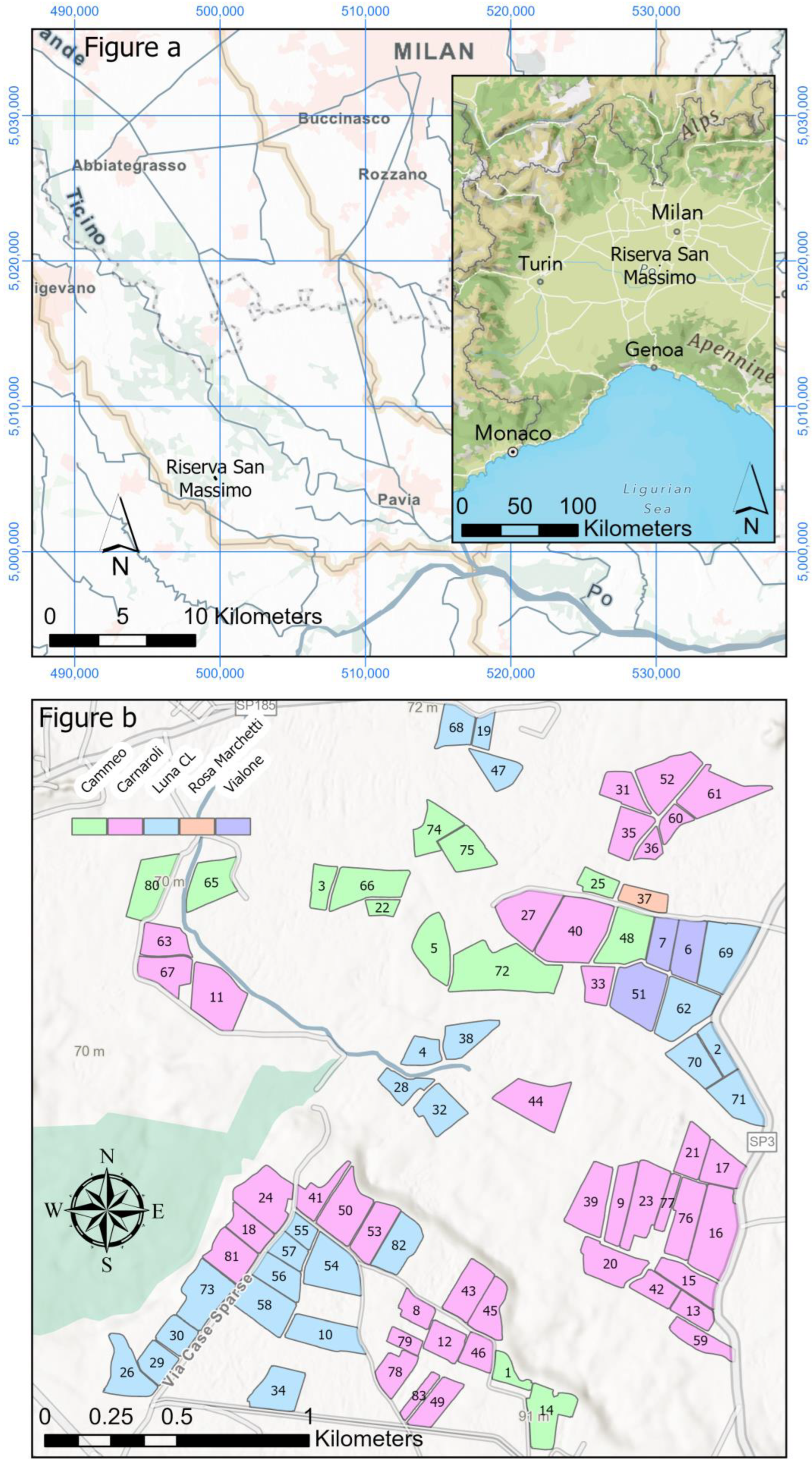
Figure 1. (a) “Riserva San Massimo” farm in Italy and (b) its rice varieties.
Geosciences 15 00184 g001
Figure 2. VRA during fertilization—field work at “Riserva San Massimo”. (a) Prescription map onboard; (b) regulator management; (c) tractor spreading fertilizer.
Geosciences 15 00184 g002
Figure 3. PlanetScope (3 m) and Sentinel-2 (10 m) acquisition compared for spatial resolution—standard colors, RGB.
Geosciences 15 00184 g003
Figure 4. PlanetScope (3 m) and Sentinel-2 (10 m) compared through Color Infrared [109,110,111] (CIR).
Geosciences 15 00184 g004
Figure 5. Alignment scheme presented in this paper.
Geosciences 15 00184 g005
Figure 6. Crops as in Figure 1b: five crops chosen to be compared through their spectral profiles.
Geosciences 15 00184 g006
Figure 7. Electromagnetic spectrum by Frank Horst [133].
Geosciences 15 00184 g007
Figure 8. Sentinel-2 (11 May 2022)—spectral profile for five crops, as shown in Figure 6. Table includes the bands’ (S2A) central wavelength (nm), their bandwidth, and spatial resolution (m). Research highlighted bands: Blue, Green, Red, RedEdge, NIR.
Geosciences 15 00184 g008
Figure 9. PlanetScope (11 May 2022)—spectral profile for five crops, as shown in Figure 6. Table includes bands’ (S2A) central wavelength (nm), bandwidth, and spatial resolution (m). Research highlighted bands: Blue, Green, Red, RedEdge, NIR.
Geosciences 15 00184 g009
Figure 10. Sentinel-2 (15 July 2022)—spectral profile for five crops, as shown in Figure 6. Table includes bands’ (S2A) central wavelength (nm), bandwidth, and spatial resolution (m). Research highlighted bands: Blue, Green, Red, RedEdge, NIR.
Geosciences 15 00184 g010
Figure 11. PlanetScope 15 July 2022—spectral profile for five crops, as shown in Figure 6. Table includes bands’ (S2A) central wavelength (nm), bandwidth, and spatial resolution (m). Research highlighted bands: Blue, Green, Red, RedEdge, NIR.
Geosciences 15 00184 g011
Figure 12. Red band calibration for 11 May 2022—Matlab Output with RMSE and MAE. Red: PlanetScope values >> Sentinel-2 values; Blue: Sentinel-2 values >> PlanetScope values; Green and Yellow: the values exhibit a good degree of similarity proportional to the magnitude of differences within the spectral channel.
Geosciences 15 00184 g012
Figure 13. 11 May 2022—Red difference raster between PlanetScope and Sentinel-2.
Geosciences 15 00184 g013
Figure 14. Red band calibration for 15 July 2022—Matlab Output with RMSE and MAE. Red: PlanetScope values >> Sentinel-2 values; Blue: Sentinel-2 values >> PlanetScope values; Green and Yellow: the values exhibit a good degree of similarity proportional to the magnitude of differences within the spectral channel.
Geosciences 15 00184 g014
Figure 15. 15 July 2022—Red difference raster between PlanetScope and Sentinel-2.
Geosciences 15 00184 g015
Figure 16. Green band calibration for 11 May 2022—Matlab Output with RMSE and MAE. Red: PlanetScope values >> Sentinel-2 values; Blue: Sentinel-2 values >> PlanetScope values; Green and Yellow: the values exhibit a good degree of similarity proportional to the magnitude of differences within the spectral channel.
Geosciences 15 00184 g016
Figure 17. 11 May 2022—Green difference raster between PlanetScope and Sentinel-2.
Geosciences 15 00184 g017
Figure 18. Green band calibration for 15 July 2022—Matlab Output with RMSE and MAE. Red: PlanetScope values >> Sentinel-2 values; Blue: Sentinel-2 values >> PlanetScope values; Green and Yellow: the values exhibit a good degree of similarity proportional to the magnitude of differences within the spectral channel.
Geosciences 15 00184 g018
Figure 19. 15 July 2022—Green difference raster between PlanetScope and Sentinel-2.
Geosciences 15 00184 g019
Figure 20. Blue band calibration for 11 May 2022—Matlab Output with RMSE and MAE. Red: PlanetScope values >> Sentinel-2 values; Blue: Sentinel-2 values >> PlanetScope values; Green and Yellow: the values exhibit a good degree of similarity proportional to the magnitude of differences within the spectral channel.
Geosciences 15 00184 g020
Figure 21. 11 May 2022—Blue difference raster between PlanetScope and Sentinel-2.
Geosciences 15 00184 g021
Figure 22. Blue band calibration for 15 July 2022—Matlab Output with RMSE and MAE. Red: PlanetScope values >> Sentinel-2 values; Blue: Sentinel-2 values >> PlanetScope values; Green and Yellow: the values exhibit a good degree of similarity proportional to the magnitude of differences within the spectral channel.
Geosciences 15 00184 g022
Figure 23. 15 July 2022—Blue difference raster between PlanetScope and Sentinel-2.
Geosciences 15 00184 g023
Figure 24. NIR band calibration for 11 May 2022—Matlab Output with RMSE and MAE. Red: PlanetScope values >> Sentinel-2 values; Blue: Sentinel-2 values >> PlanetScope values; Green and Yellow: the values exhibit a good degree of similarity proportional to the magnitude of differences within the spectral channel.
Geosciences 15 00184 g024
Figure 25. 11 May 2022—NIR difference raster between PlanetScope and Sentinel-2.
Geosciences 15 00184 g025
Figure 26. NIR band calibration for 15 July 2022—Matlab Output with RMSE and MAE. Red: PlanetScope values >> Sentinel-2 values; Blue: Sentinel-2 values >> PlanetScope values; Green and Yellow: the values exhibit a good degree of similarity proportional to the magnitude of differences within the spectral channel.
Geosciences 15 00184 g026
Figure 27. 15 July 2022—NIR difference raster between PlanetScope and Sentinel-2.
Geosciences 15 00184 g027
Figure 28. Red Edge band calibration 11 May 2022—Matlab Output with RMSE and MAE. Red: PlanetScope values >> Sentinel-2 values; Blue: Sentinel-2 values >> PlanetScope values; Green and Yellow: the values exhibit a good degree of similarity proportional to the magnitude of differences within the spectral channel.
Geosciences 15 00184 g028
Figure 29. 11 May 2022—RedEdge difference raster between PlanetScope and Sentinel-2.
Geosciences 15 00184 g029
Figure 30. Red Edge band calibration 15 July 2022—Matlab Output with RMSE and MAE. Red: PlanetScope values >> Sentinel-2 values; Blue: Sentinel-2 values >> PlanetScope values; Green and Yellow: the values exhibit a good degree of similarity proportional to the magnitude of differences within the spectral channel.
Geosciences 15 00184 g030
Figure 31. 15 July 2022—RedEdge difference raster between PlanetScope and Sentinel-2.
Geosciences 15 00184 g031
Figure 32. “Riserva San Massimo” digital terrain model—RL, Res: 5 m.
Geosciences 15 00184 g032
Table 1. Comparing use and characteristics of important indices which are influenced by this research.
IndexApplicationsBandDetection Capability
NDVI
N I R R e d N I R + R e d
Assessing vegetation presence, density, vigor, and overall health. Widely used in agriculture, forestry, and ecological monitoring.Red, NIRQuantifies the “greenness” of vegetation. Strongly correlated with chlorophyll content, leaf area index (LAI), and photosynthetic activity. Can saturate in dense vegetation.
NDRE
N I R R e d   E d g e N I R + R e d   E d g e
Assessing vegetation health, chlorophyll content, and nitrogen status, particularly useful in mid-to-late growth stages or dense canopies.Red Edge, NIRSensitive to chlorophyll concentration deeper within the canopy. Less prone to saturation than NDVI in dense vegetation. Often used as an indicator of plant stress or nitrogen levels.
Iron Oxide Ratio
R e d B l u e
Highlighting areas with surface iron oxide (Fe3+) staining (e.g., hematite, goethite). Used in geological mapping and mineral exploration.Red, BlueIdentifies surfaces exhibiting strong red reflectance relative to blue reflectance, characteristic of reddish iron oxide minerals or weathered lateritic soils.
Coloration Index
R e d G r e e n R e d + G r e e n
Identifying areas dominated by reddish/yellowish coloration, often associated with ferric iron (Fe3+) minerals like limonite, jarosite, goethite. Used in hydrothermal alteration mapping.Red, GreenDetects surfaces where red reflectance significantly exceeds green reflectance, indicating the presence of various ferric iron minerals common in altered or weathered zones.
Table 2. Spectral channels used during alignment.
BandsSentinel-2PlanetScope
BlueBand 2—Blue Band 2—Blue
GreenBand 3—GreenBand 4—Green
RedBand 4—RedBand 6—Red
Red EdgeBand 5—RedEdge 705Band 7—RedEdge
NIRBand 8—NIRBand 8—NIR
Disclaimer/Publisher’s Note: The statements, opinions and data contained in all publications are solely those of the individual author(s) and contributor(s) and not of MDPI and/or the editor(s). MDPI and/or the editor(s) disclaim responsibility for any injury to people or property resulting from any ideas, methods, instructions or products referred to in the content.