


Seismic Facies Classification of Salt Structures and Sediments in the Northern Gulf of Mexico Using Self-Organizing Maps


Abstract
1. Introduction
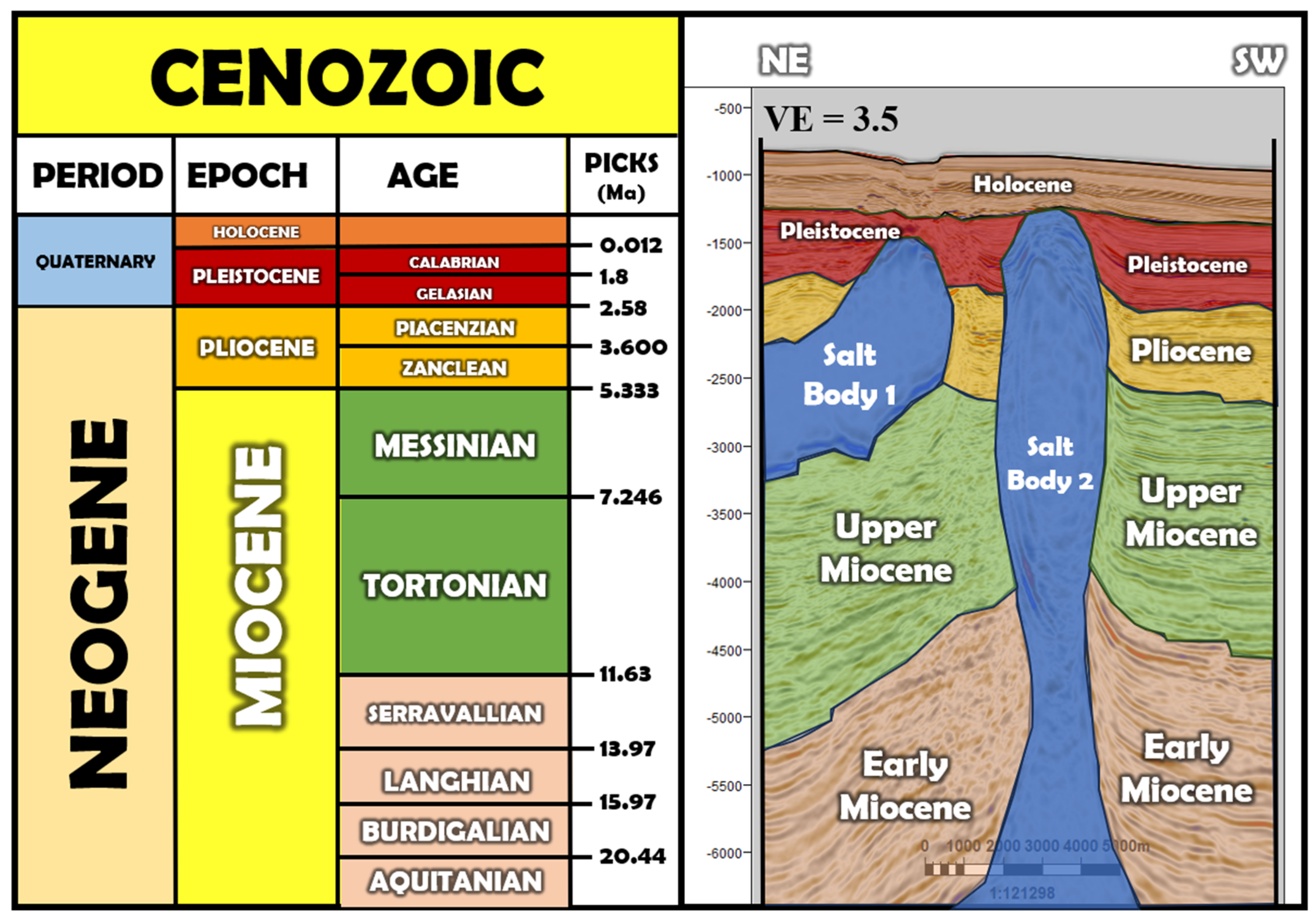
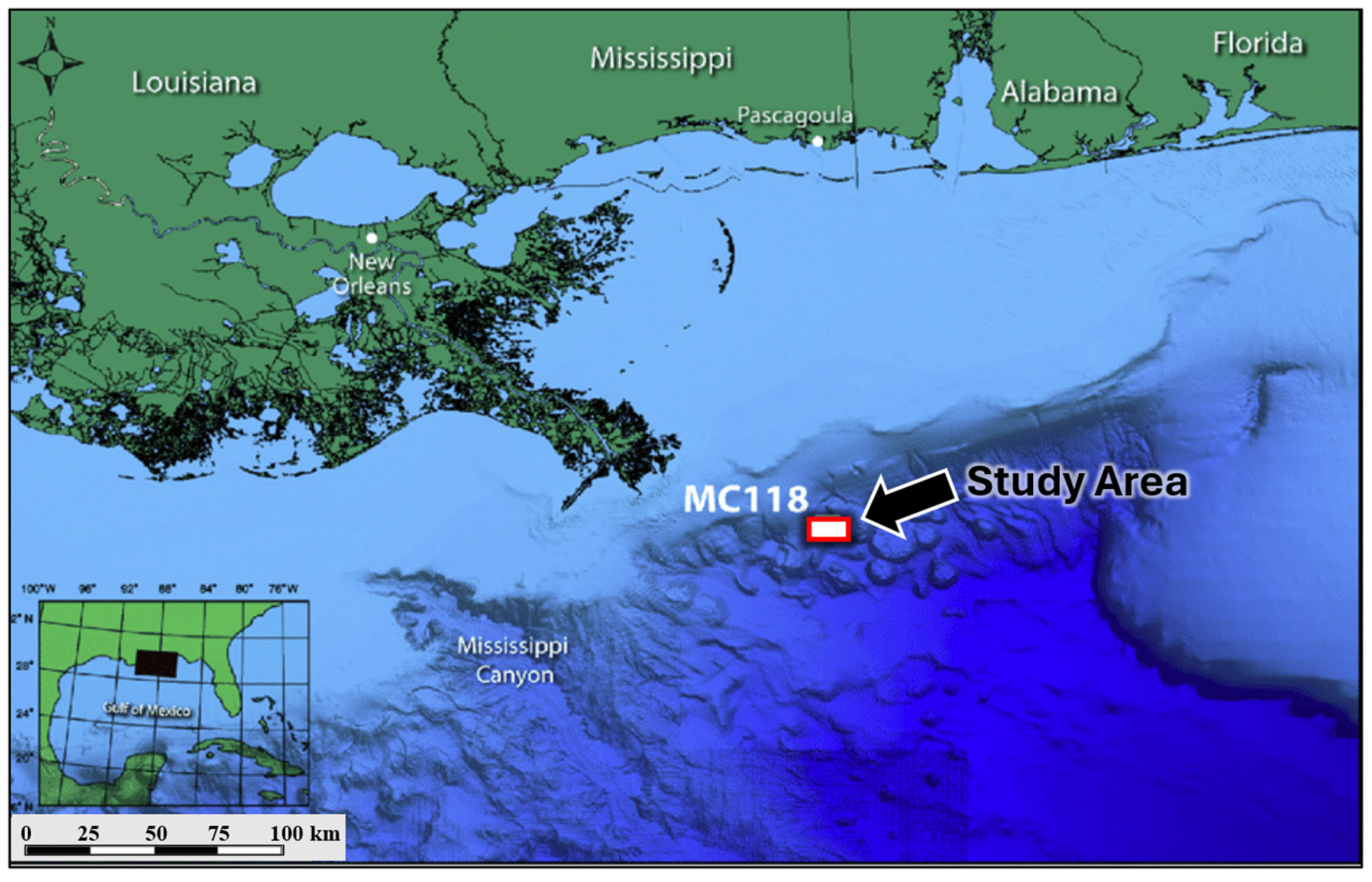
2. Geologic Setting
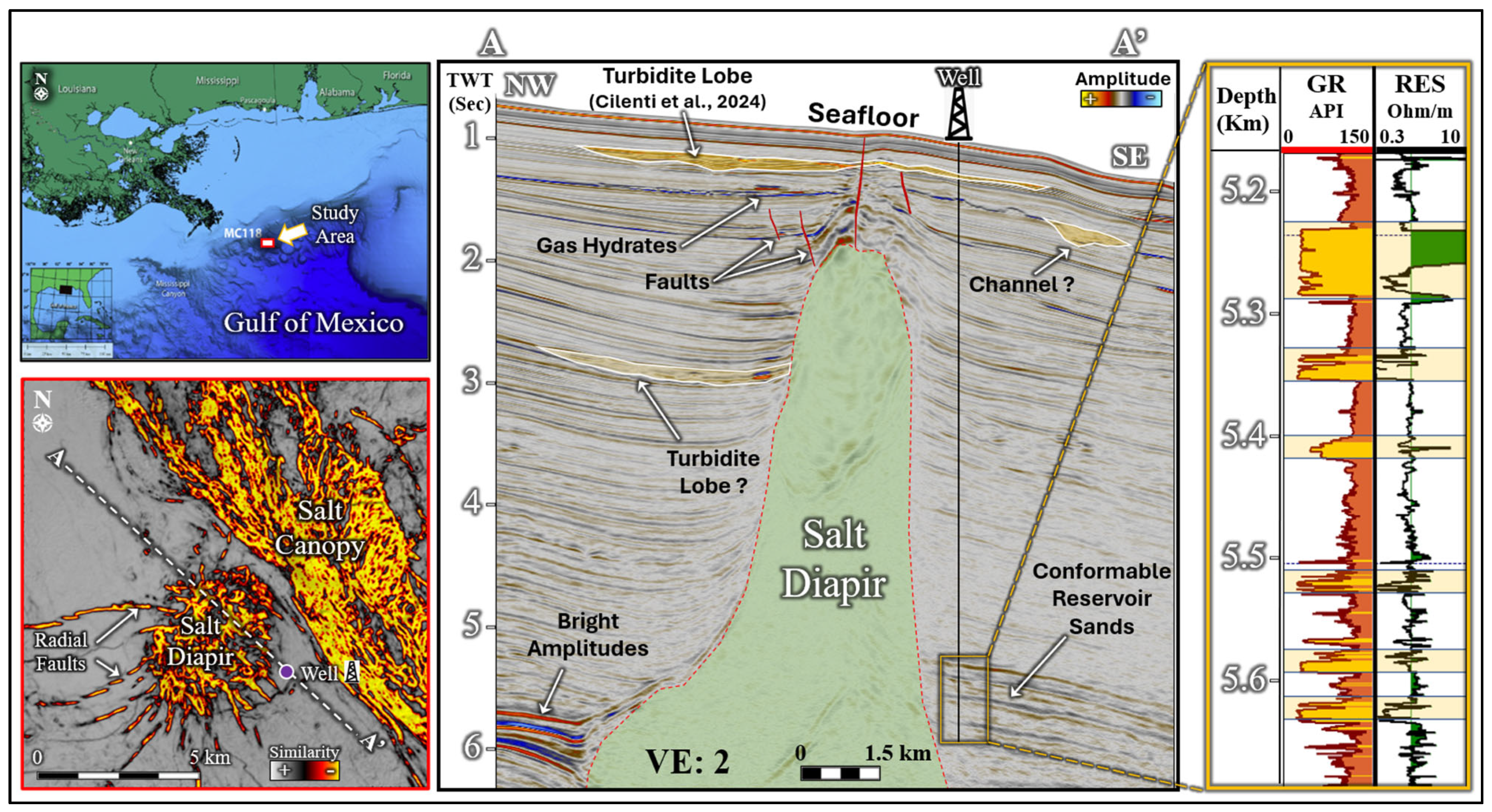
3. Datasets
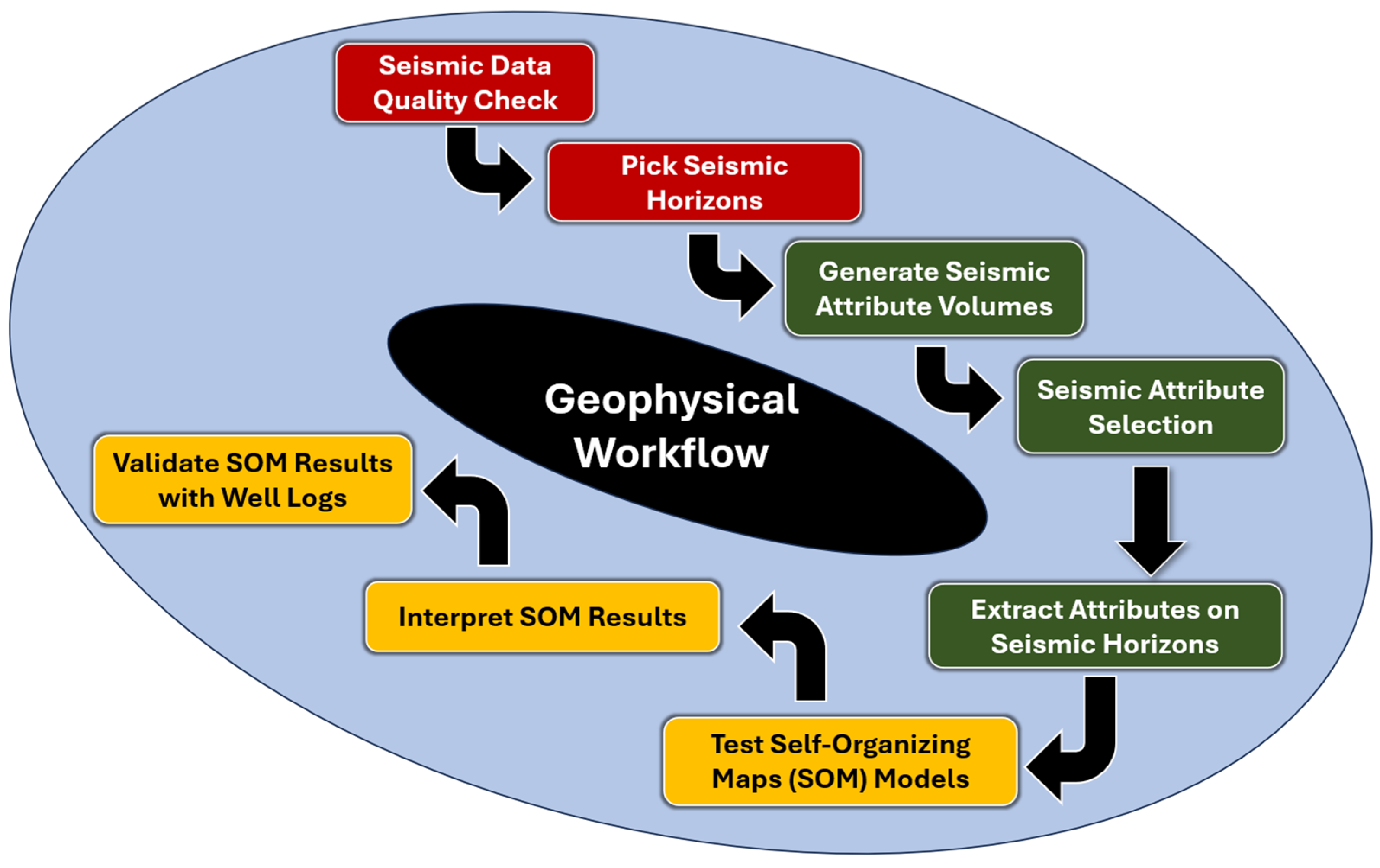
4. Methodology
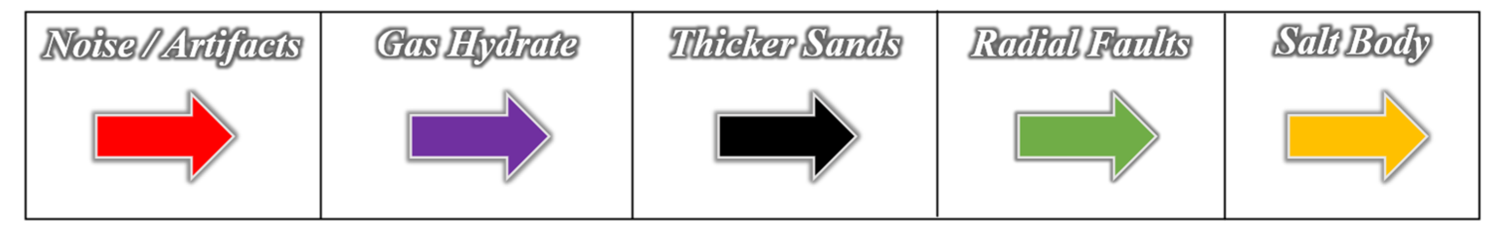
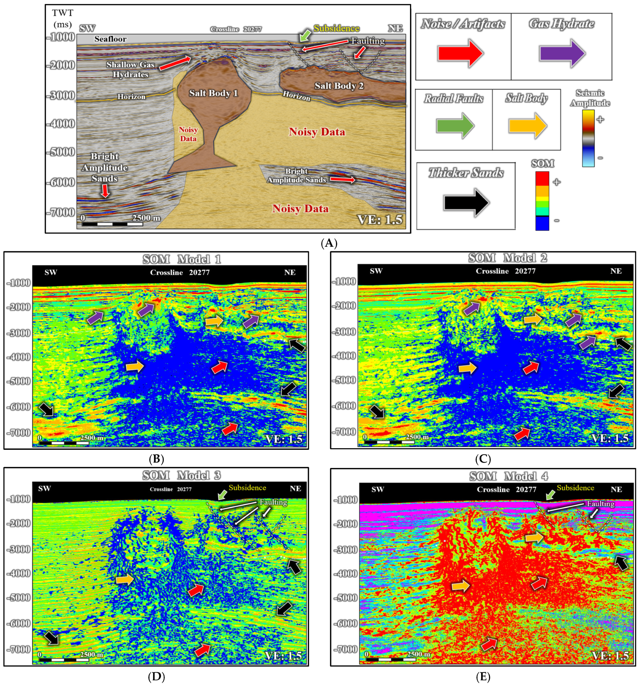
4.1. Seismic Facies Identification
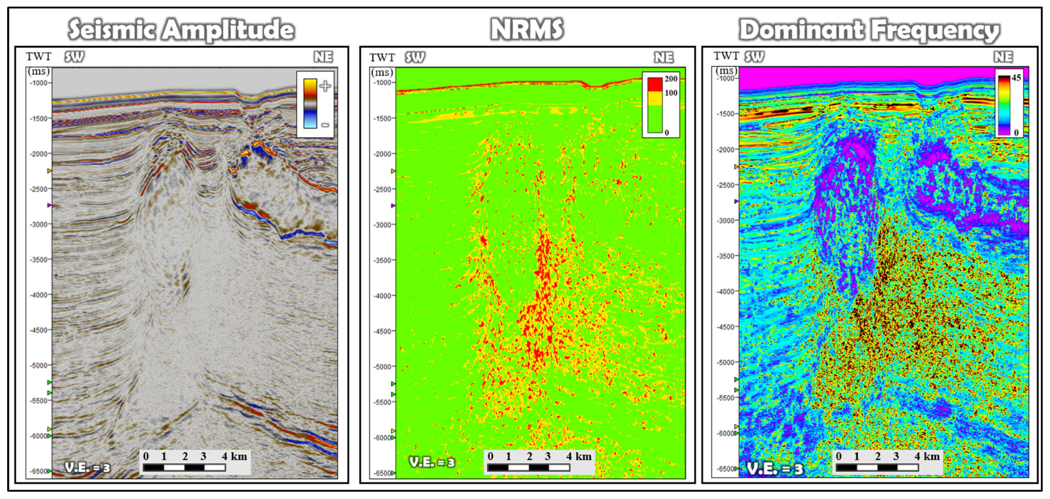
4.2. Seismic Data Quality Check
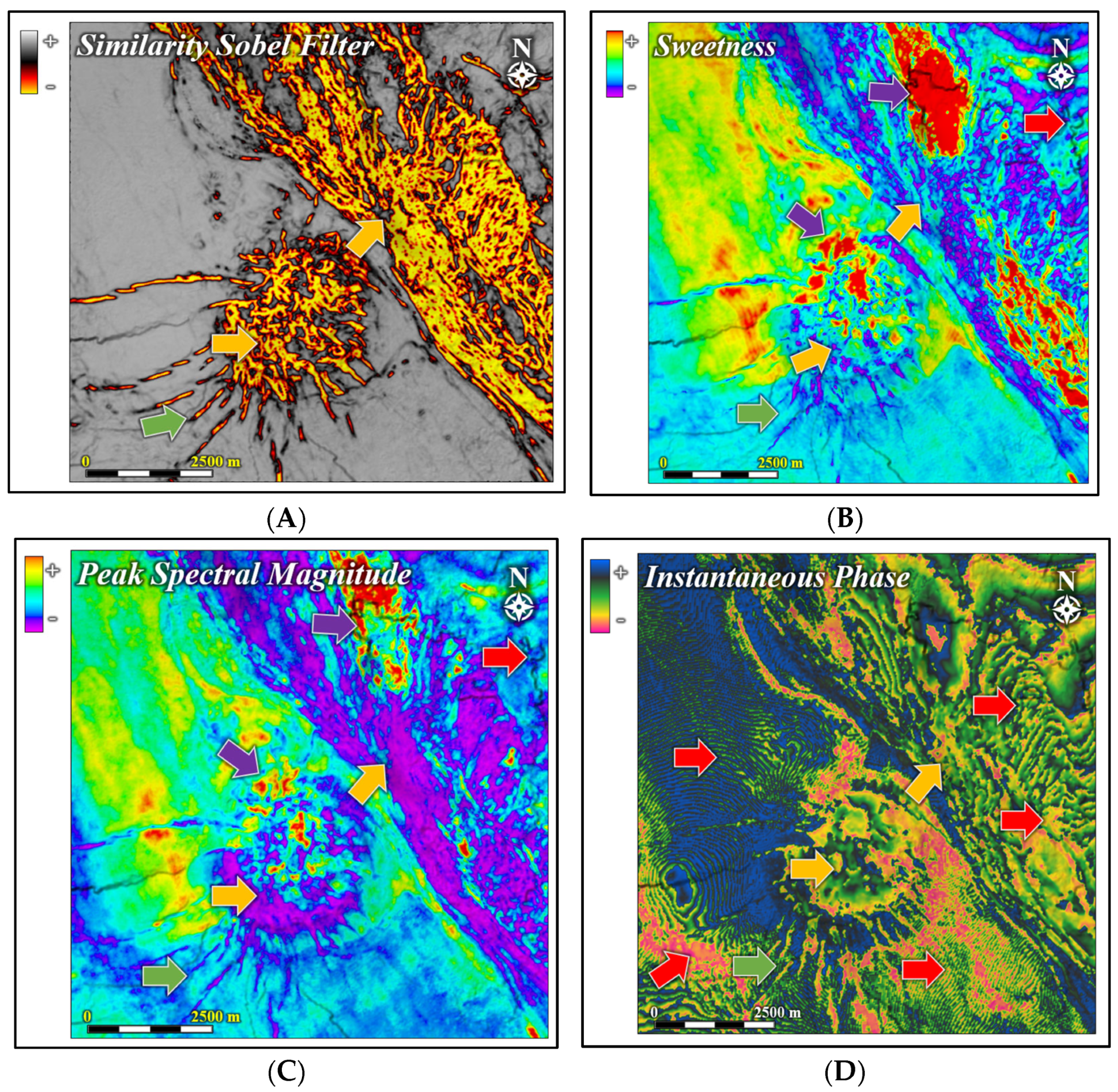
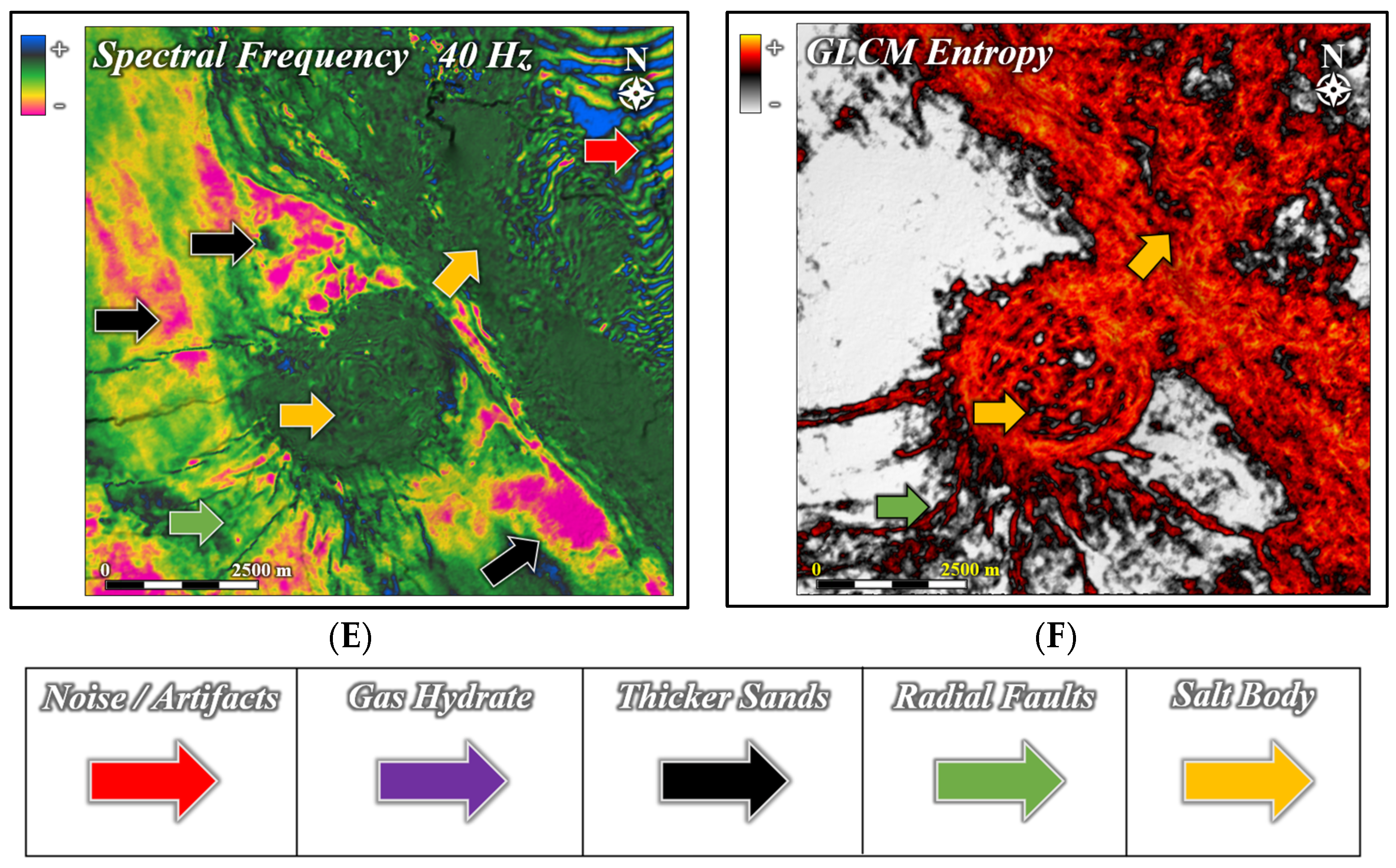
4.3. Seismic Attribute Selection
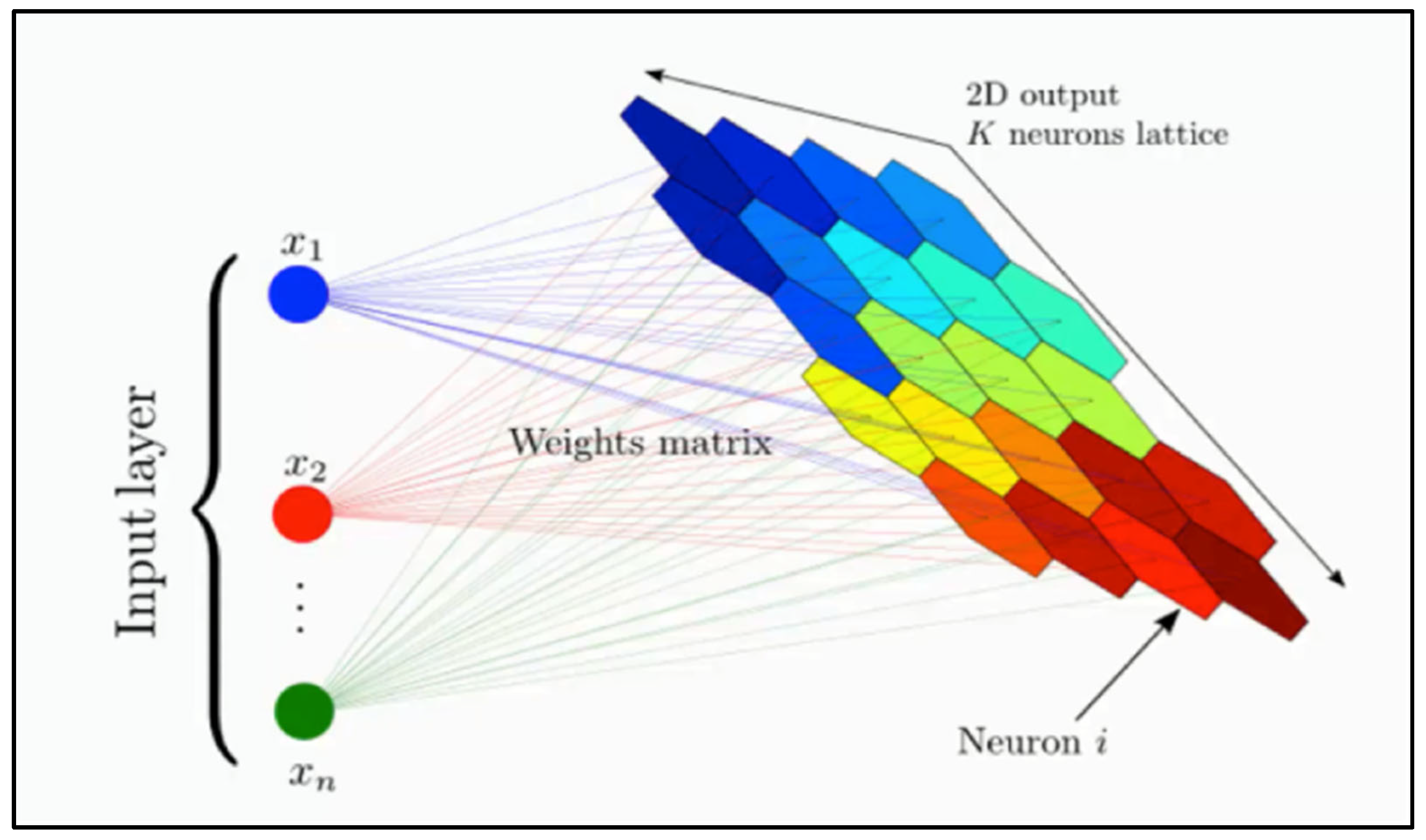
4.4. Self-Organizing Map Algorithm
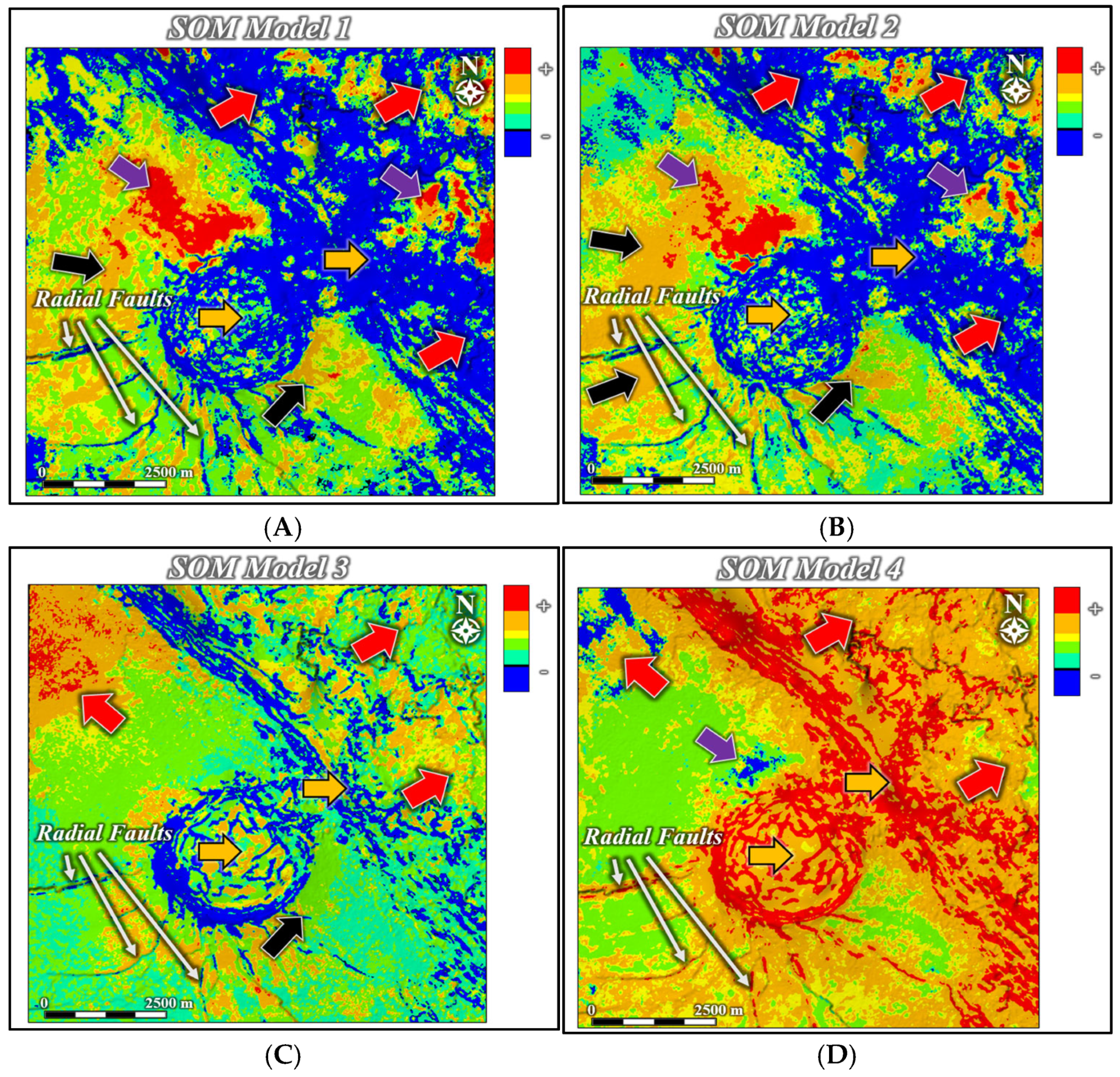
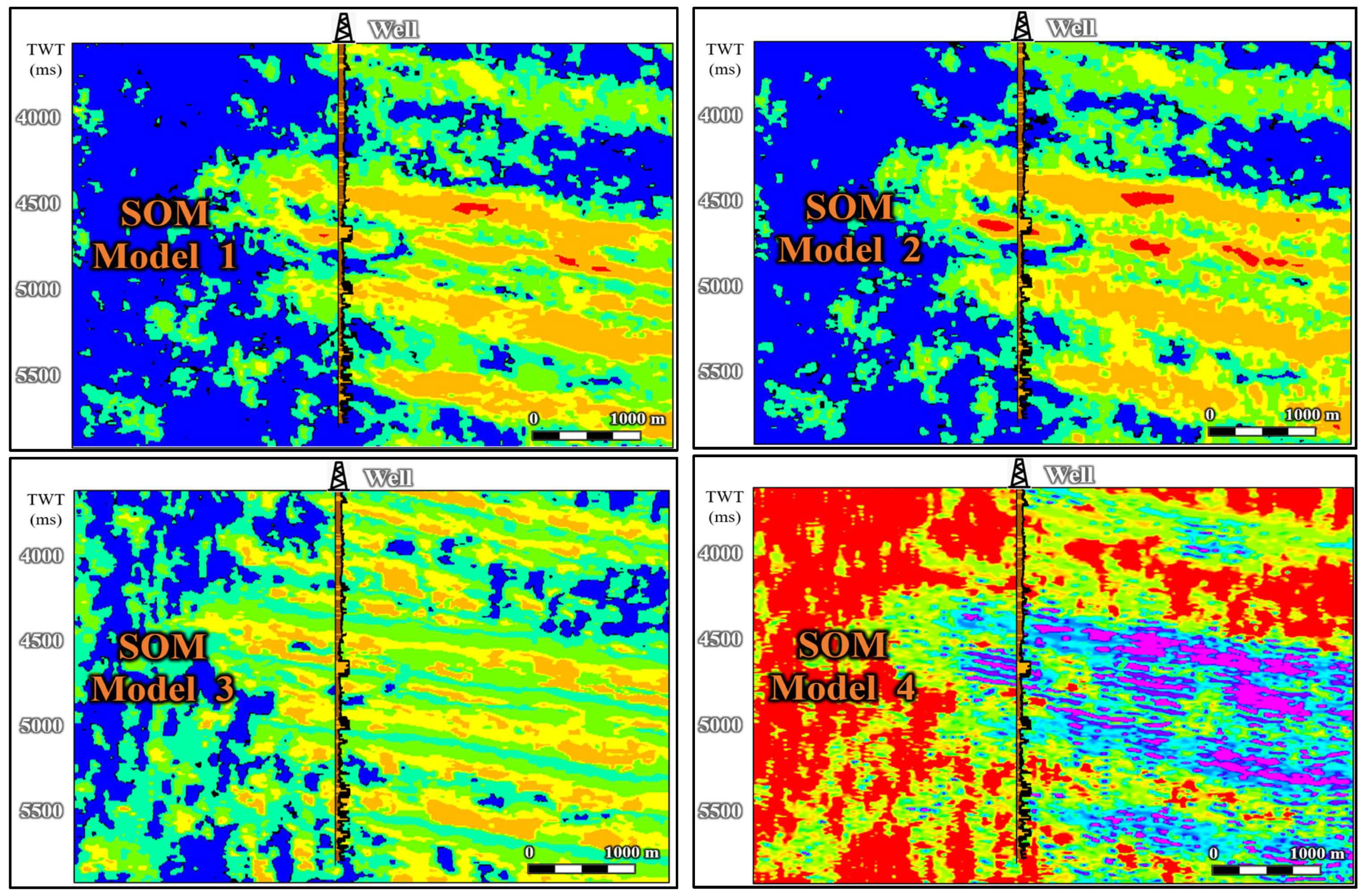
5. Results
6. Discussion
7. Conclusions
Author Contributions
Funding
Data Availability Statement
Acknowledgments
Conflicts of Interest
Abbreviations
| ML | Machine Learning |
| SOM | Self-Organizing Maps |
| MC-118 | Mississippi Canyon, Block 118 |
References
- Sambo, C.; Dudun, A.; Samuel, S.A.; Esenenjor, P.; Muhammed, N.S.; Haq, B. A review on worldwide underground hydrogen storage operating and potential fields. Int. J. Hydrogen Energy 2022, 47, 22840–22880. [Google Scholar] [CrossRef]
- Askarova, A.; Mukhametdinova, A.; Markovic, S.; Khayrullina, G.; Afanasev, P.; Popov, E.; Mukhina, E. An overview of geological CO2 sequestration in oil and gas reservoirs. Energies 2023, 16, 2821. [Google Scholar] [CrossRef]
- Osahon, U.; Efetobore, M.O.G. Reservoir Characterization: Enhancing Accuracy through Advanced Rock Physics Techniques. J. Geosci. 2023, 11, 67–78. [Google Scholar] [CrossRef]
- Vodopić, F.; Vulin, D.; Karasalihović Sedlar, D.; Jukić, L. Enhancing Carbon Capture and Storage Deployment in the EU: A Sectoral Analysis of a Ton-Based Incentive Strategy. Sustainability 2023, 15, 15717. [Google Scholar] [CrossRef]
- Jia, A.; He, D.; Jia, C. Advances and challenges of reservoir characterization: A review of the current state-of-the-art. In Earth Sciences; BoD - Books on Demand GmbH: Norderstedt, Germany, 2012; Volume 1. [Google Scholar]
- Samuel, S.A.; Zhang, R. Total Organic Carbon Content Estimation of Bakken Formation, Kevin-Sunburst Dome, Montana using Post-Stack Inversion, Passey (DLogR) Method and Multi-Attribute Analysis. In Proceedings of the SPE/AAPG/SEG Unconventional Resources Technology Conference, Houston, TX, USA, 26–28 July 2021; URTEC: Tulsa, OK, USA, 2021; p. D021S047R003. [Google Scholar]
- Hampson, D.P.; Schuelke, J.S.; Quirein, J.A. Use of multiattribute transforms to predict log properties from seismic data. Geophysics 2001, 66, 220–236. [Google Scholar] [CrossRef]
- Satinder, C.; Marfurt, K.J. Seismic attributes—A historical perspective. Geophysics 2005, 70, 3SO–28SO. [Google Scholar]
- Oumarou, S.; Mabrouk, D.; Tabod, T.C.; Marcel, J.; Ngos, S., III; Essi, J.M.A.; Kamguia, J. Seismic attributes in reservoir characterization: An overview. Arab. J. Geosci. 2021, 14, 402. [Google Scholar] [CrossRef]
- Roden, R.; Smith, T.; Sacrey, D. Geologic pattern recognition from seismic attributes: Principal component analysis and self-organizing maps. Interpretation 2015, 3, SAE59–SAE83. [Google Scholar] [CrossRef]
- La Marca, K. Seismic Attribute Optimization with Unsupervised Machine Learning Techniques for Deepwater Seismic Facies Interpretation: Users vs Machines (2020). Available online: https://shareok.org/items/2de83777-843d-4ea0-a0c7-332351c7fc0a (accessed on 10 May 2025).
- La Marca, K.; Bedle, H. Deepwater seismic facies and architectural element interpretation aided with unsupervised machine learning techniques: Taranaki basin, New Zealand. Mar. Pet. Geol. 2022, 136, 105427. [Google Scholar] [CrossRef]
- La Marca, K.; Bedle, H. User vs. machine-based seismic attribute selection for unsupervised machine learning techniques: Does human insight provide better results than statistically chosen attributes? In Advances in Subsurface Data Analytics; Elsevier: Amsterdam, The Netherlands, 2022; pp. 3–30. [Google Scholar]
- Zhao, T.; Jayaram, V.; Roy, A.; Marfurt, K.J. A comparison of classification techniques for seismic facies recognition. Interpretation 2015, 3, SAE29–SAE58. [Google Scholar] [CrossRef]
- Kohonen, T. Self-organized formation of topologically correct feature maps. Biol. Biol. Cybern. 1982, 43, 59–69. [Google Scholar] [CrossRef]
- Kohonen, T.; Kohonen, T. The basic SOM. In Self-Organizing Maps; Springer: Berlin, Heidelberg, 2001; pp. 105–176. [Google Scholar]
- Rauber, A.; Merkl, D.; Dittenbach, M. The growing hierarchical self-organizing map: Exploratory analysis of high-dimensional data. IEEE Trans. Neural Netw. 2002, 13, 1331–1341. [Google Scholar] [CrossRef]
- Saraswat, P.; Sen, M.K. Artificial immune-based self-organizing maps for seismic-facies analysis. Geophysics 2012, 77, O45–O53. [Google Scholar] [CrossRef]
- Astudillo, C.A.; Oommen, B.J. Topology-oriented self-organizing maps: A survey. Pattern Anal. Appl. 2014, 17, 223–248. [Google Scholar] [CrossRef]
- Zhao, T.; Li, F.; Marfurt, K.J. Constraining self-organizing map facies analysis with stratigraphy: An approach to increase the credibility in automatic seismic facies classification. Interpretation 2017, 5, T163–T171. [Google Scholar] [CrossRef]
- Christianson, P.A.; Murray, P.E. Investigating active deep-water sedimentation near a gas hydrate system with high-resolution seismic data. In Proceedings of the 2007 SEG Annual Meeting, San Antonio, TX, USA, 23–28 September 2007. [Google Scholar]
- McGee, T.; Macelloni, L.; Lutken, C.; Bosman, A.; Brunner, C.; Rogers, R.; Woolsey, J.R. Hydrocarbon gas hydrates in sediments of the Mississippi Canyon area, Northern Gulf of Mexico. Geol. Soc. Lond. Spec. Publ. 2009, 319, 29–49. [Google Scholar] [CrossRef]
- Macelloni, L.; Simonetti, A.; Knapp, J.H.; Knapp, C.C.; Lutken, C.B.; Lapham, L.L. Multiple resolution seismic imaging of a shallow hydrocarbon plumbing system, Woolsey Mound, Northern Gulf of Mexico. Mar. Pet. Geol. 2012, 38, 128–142. [Google Scholar] [CrossRef]
- Ingram, W.C.; Meyers, S.R.; Martens, C.S. Chemostratigraphy of deep-sea Quaternary sediments along the Northern Gulf of Mexico Slope: Quantifying the source and burial of sediments and organic carbon at Mississippi Canyon 118. Mar. Pet. Geol. 2013, 46, 190–200. [Google Scholar] [CrossRef]
- Pizzi, M.; Macelloni, L.; Lutken, C.B.; D’Emidio, M. Temporal Evolution of MC118 Woolsey Mound Seep Activity: Constraints from Analysis of Small-Scale Salt-Induced Sediment Deformation 2012. Available online: https://www.researchgate.net/publication/295920286_Temporal_Evolution_of_MC118_Woolsey_Mound_seep_activity_constraints_from_analysis_of_small-scale_salt-induced_sediment_deformation (accessed on 10 May 2025).
- Salazar, J.A.; Knapp, J.H.; Knapp, C.C.; Pyles, D.R. Salt tectonics and Pliocene stratigraphic framework at MC-118, Gulf of Mexico: An integrated approach with application to deep-water confined structures in salt basins. Mar. Pet. Geol. 2014, 50, 51–67. [Google Scholar] [CrossRef]
- Offshore Engineer. ConocoPhillips Misses in GoM. 2005. Available online: https://www.oedigital.com/news/452843-conocophillips-misses-in-gom (accessed on 10 February 2025).
- Simonetti, A.; Knapp, J.H.; Sleeper, K.; Lutken, C.B.; Macelloni, L.; Knapp, C.C. Spatial distribution of gas hydrates from high-resolution seismic and core data, Woolsey Mound, Northern Gulf of Mexico. Mar. Pet. Geol. 2013, 44, 21–33. [Google Scholar] [CrossRef]
- Fisher, C.; Roberts, H.; Cordes, E.; Bernard, B. Cold seeps and associated communities of the Gulf of Mexico. Oceanography 2007, 20, 118–129. [Google Scholar] [CrossRef]
- Bouma, A.H.; Bryant, W.R. Physiographic features on the northern Gulf of Mexico continental slope. Geo-Mar. Lett. 1994, 14, 252–263. [Google Scholar] [CrossRef]
- Sleeper, K.; Lowrie, A.; Bosman, A.; Macelloni, L.; Swann, C.T. Bathymetric mapping and high-resolution seismic profiling by AUV in MC 118 (Gulf of Mexico). In Proceedings of the Offshore Technology Conference, Houston, TX, USA, 1–4 May 2006; p. OTC-18113. [Google Scholar]
- Alam, S.; Knapp, C.C.; Knapp, J.H.; Simonetti, A. Temporal and spatial characterization of a thermogenic, fault-controlled gas hydrate system, Woolsey Mound, Gulf of Mexico. Interpretation 2024, 12, T221–T232. [Google Scholar] [CrossRef]
- Alam, S.; Knapp, C.; Knapp, J. Three-Dimensional Amplitude versus Offset Analysis for Gas Hydrate Identification at Woolsey Mound: Gulf of Mexico. GeoHazards 2024, 5, 271–285. [Google Scholar] [CrossRef]
- Biondi, B.L. 3D Seismic Imaging; Society of Exploration Geophysicists: Houston, TX, USA, 2006. [Google Scholar]
- SEG Wiki. Gulf of Mexico 2019. Available online: https://wiki.seg.org/wiki/Gulf_of_Mexico (accessed on 1 November 2023).
- Samuel, S.A.; Knapp, C.C.; Knapp, J.H. Volumetric carbon storage capacity estimation at Mississippi Canyon Block 118 in the Gulf of Mexico using Post-Stack Seismic Inversion. Int. J. Greenh. Gas Control 2025, 141, 104319. [Google Scholar] [CrossRef]
- Cilenti, F.; Oppo, D.; Macelloni, L. Controls on fluid discharge at cold seep-hydrate systems: 4D seismic monitoring of Woolsey Mound, Gulf of Mexico. Earth Planet. Sci. Lett. 2024, 648, 119087. [Google Scholar] [CrossRef]
- Mitchum, R.M., Jr.; Vail, P.R.; Sangree, J.B. Seismic stratigraphy and global changes of sea level: Part 6. Stratigraphic interpretation of seismic reflection patterns in depositional sequences: Section 2. Application of seismic reflection configuration to stratigraphic interpretation. AAPG Mem. 1977, 26, 117–133. [Google Scholar]
- Salazar Florez, D.; Bedle, H. Study on the parameterization response of probabilistic neural networks for seismic facies classification in the Gulf of Mexico. Interpretation 2022, 10, T1–T23. [Google Scholar] [CrossRef]
- Sangree, J.B.; Widmier, J.M. Interpretation of depositional facies from seismic data. Geophysics 1979, 44, 131–160. [Google Scholar] [CrossRef]
- Roksandić, M.M. Seismic facies analysis concepts. Geophys. Prospect. 1978, 26, 383–398. [Google Scholar] [CrossRef]
- Brown, A.R. Interpretation of Three-Dimensional Seismic Data; Society of Exploration Geophysicists and American Association of Petroleum Geologists: Houston, TX, USA, 2011. [Google Scholar]
- Umoren, E.B.; George, N.J. Time lapse (4D) and AVO analysis: A case study of Gullfaks field, Northern North Sea. NRIAG J. Astron. Geophys. 2018, 7, 62–77. [Google Scholar] [CrossRef]
- Hart, B.S. Definition of subsurface stratigraphy, structure and rock properties from 3-D seismic data. Earth-Sci. Rev. 1999, 47, 189–218. [Google Scholar] [CrossRef]
- Taner, M.T.; Schuelke, J.S.; O’Doherty, R.; Baysal, E. Seismic attributes revisited. In SEG Technical Program Expanded Abstracts; Society of Exploration Geophysicist: Houston, TX, USA, 1994; pp. 1104–1106. [Google Scholar]
- Barnes, A.E. A tutorial on complex seismic trace analysis. Geophysics 2007, 72, W33–W43. [Google Scholar] [CrossRef]
- Chopra, S.; Marfurt, K.J. Seismic Attributes for Prospect Identification and Reservoir Characterization; Society of Exploration Geophysicists and European Association of Geoscientists and Engineers: Houston, TX, USA, 2007. [Google Scholar]
- SEG Wiki. Self-Organizing Map and Multi-Attribute Analysis 2018. Available online: https://wiki.seg.org/wiki/Self_Organizing_Map_and_Multi-attribute_Analysis (accessed on 1 November 2023).
- Chopra, S.; Marfurt, K. Seismic Curvature Attributes for Mapping Faults/Fractures, and Other Stratigraphic (2007b). Available online: https://csegrecorder.com/articles/view/seismic-curvature-attributes-for-mapping-faults-fractures-and-other (accessed on 10 May 2025).
- Chopra, S.; Marfurt, K. Curvature attribute applications to 3D surface seismic data. Lead. Edge 2007, 26, 404–414. [Google Scholar] [CrossRef]
- Subrahmanyam, D.; Rao, P.H. Seismic Attributes-A Review. In Proceedings of the 7th International Conference and Exposition on Petroleum Geophysics, Hyderabad, India, January 2008; Available online: https://spgindia.org/2008/398.pdf (accessed on 10 May 2025).
- Gao, D. Integrating 3D seismic curvature and curvature gradient attributes for fracture characterization: Methodologies and interpretational implications. Geophysics 2013, 78, O21–O31. [Google Scholar] [CrossRef]
- Hutchinson, B. Application and Limitations of Seismic Attributes on 2D Reconnaissance Surveys 2016. Available online: https://mcee.ou.edu/aaspi/AASPI_Theses/2016_AASPI_Theses/2016_Hutchinson_Bryce_Thesis.pdf (accessed on 10 May 2025).
- Qi, X.; Marfurt, K. Volumetric aberrancy to map subtle faults and flexures. Interpretation 2018, 6, T349–T365. [Google Scholar] [CrossRef]
- Bhattacharya, S.; Verma, S. Application of volumetric seismic attributes for complex fault network characterization on the North Slope, Alaska. J. Nat. Gas Sci. Eng. 2019, 65, 56–67. [Google Scholar] [CrossRef]
- Verma, S.; Bhattacharya, S. 3D seismic attribute visualization and analysis for fault characterization. In Developments in Structural Geology and Tectonics; Elsevier: Amsterdam, The Netherlands, 2024; Volume 6, pp. 37–55. [Google Scholar]
- James, G.; Partyka, G. Processing and interpretational aspects of spectral decomposition. SEG Tech. Program Expand. Abstr. 1997, 1997, 1055–1058. [Google Scholar]
- Partyka, G.; Gridley, J.; Lopez, J. Interpretational applications of spectral decomposition in reservoir characterization. Lead. Edge 1999, 18, 353–360. [Google Scholar] [CrossRef]
- Partyka, G. The birth of spectral decomposition. Lead. Edge 2007, 26, 1624. [Google Scholar] [CrossRef]
- Partyka, G.A.; Bush, M.D.; Garossino, P.G.; Gutowski, P.R. Spectral Decomposition. In Interpretation of Three-Dimensional Seismic Data; American Association of Petroleum Geologists: Tulsa, OK, USA, 2011; pp. 295–308. [Google Scholar]
- White Roy, E. Properties of instantaneous seismic attributes. Lead. Edge 1991, 10, 26–32. [Google Scholar] [CrossRef]
- Chopra, S.; Marfurt, K.J. Emerging and future trends in seismic attributes. Lead. Edge 2008, 27, 298–318. [Google Scholar] [CrossRef]
- Laughlin, K.; Garossino, P.; Partyka, G. GCSpectral Decomposition for Seismic Stratigraphic Patterns. 2003. Available online: https://www.searchanddiscovery.com/pdfz/documents/geophysical/2003/laughlin/images/laughlin.pdf.html (accessed on 10 May 2025).
- Naseer, M.T.; Asim, S. Application of instantaneous spectral analysis and acoustic impedance wedge modeling for imaging the thin beds and fluids of fluvial sand systems of Indus Basin, Pakistan. J. Earth Syst. Sci. 2018, 127, 97. [Google Scholar] [CrossRef]
- Nanda, N.C. Analysing seismic attributes. In Seismic Data Interpretation and Evaluation for Hydrocarbon Exploration and Production: A Practitioner’s Guide; Springer International Publishing: Cham, Switzerland, 2021; pp. 205–222. [Google Scholar]
- Silver, C.; La Marca-Molina, K.; Bedle, H. Seismic geomorphology of deep-water channel systems in the southern Taranaki Basin. In SEG Technical Program Expanded Abstracts; Society of Exploration Geophysicists: Houston, TX, USA, 2019; pp. 2018–2022. [Google Scholar]
- La Marca-Molina, K.; Silver, C.; Bedle, H.; Slatt, R. Seismic facies identification in a deepwater channel complex applying seismic attributes and unsupervised machine learning techniques. A case study in the Taranaki Basin, New Zealand. In SEG Technical Program Expanded Abstracts; Society of Exploration Geophysicists: Houston, TX, USA, 2019; pp. 2059–2063. [Google Scholar]
- Verma, S.; Scipione, M. The early Paleozoic structures and its influence on the Permian strata, Midland Basin: Insights from multi-attribute seismic analysis. J. Nat. Gas Sci. Eng. 2020, 82, 103521. [Google Scholar] [CrossRef]
- Olaleye, O.K.; Enikanselu, P.A.; Ayuk, M.A. Characterization of reservoir sands using 3D seismic attributes in the coastal swamp area of Niger Delta Basin. J. Pet. Explor. Prod. Technol. 2021, 11, 3995–4004. [Google Scholar] [CrossRef]
- SuperDataScience Team. Self-Organizing Maps (SOM’s)—How Do Self-Organizing Maps Work? 2018. Available online: https://www.superdatascience.com/blogs/self-organizing-maps-soms-how-do-self-organizing-maps-work (accessed on 27 October 2023).
- Matos, M.C.D.; Marfurt, K.J.; Johann, P.R. Seismic interpretation of self-organizing maps using 2D color displays. Rev. Bras. Geof. 2010, 28, 631–642. [Google Scholar] [CrossRef]
- Smith, T.; Treitel, S. Introduction to Self-Organizing Maps in Multi-Attribute Seismic Data; Geophysical Society of Houston: Houston, TX, USA, 2011. [Google Scholar]
- McMullen Patrick, R. A Kohonen self-organizing map approach to addressing a multiple objective, mixed-model JIT sequencing problem. Int. J. Prod. Econ. 2001, 72, 59–71. [Google Scholar] [CrossRef]
- Liu, Y.; Weisberg, R.H.; Mooers, C.N. Performance evaluation of the self-organizing map for feature extraction. J. Geophys. Res. Ocean. 2006, 111. [Google Scholar] [CrossRef]
- Tasdemir, K.; Merényi, E. Exploiting data topology in visualization and clustering of self-organizing maps. IEEE Trans. Neural Netw. 2009, 20, 549–562. [Google Scholar] [CrossRef] [PubMed]
- Singh, N.; Javeed, A.; Chhabra, S.; Kumar, P. Missing value imputation with unsupervised kohonen self organizing map. In Emerging Research in Computing, Information, Communication and Applications: ERCICA 2015; Springer: New Delhi, India, 2015; Volume 1, pp. 61–76. [Google Scholar]
- Gu, F.; Cheung, Y.M. Self-organizing map-based weight design for decomposition-based many-objective evolutionary algorithm. IEEE Trans. Evol. Comput. 2017, 22, 211–225. [Google Scholar] [CrossRef]
- Vesanto, J.; Alhoniemi, E. Clustering of the self-organizing map. IEEE Trans. Neural Netw. 2000, 11, 586–600. [Google Scholar] [CrossRef]
- Kohonen, T. Essentials of the self-organizing map. Neural Netw. 2013, 37, 52–65. [Google Scholar] [CrossRef]
- Köhler, A.; Ohrnberger, M.; Scherbaum, F. Unsupervised pattern recognition in continuous seismic wavefield records using self-organizing maps. Geophys. J. Int. 2010, 182, 1619–1630. [Google Scholar] [CrossRef]
- Du, H.K.; Cao, J.X.; Xue, Y.J.; Wang, X.J. Seismic facies analysis based on self-organizing map and empirical mode decomposition. J. Appl. Geophys. 2015, 112, 52–61. [Google Scholar] [CrossRef]

| ATTRIBUTE CATEGORY | SEISMIC ATTRIBUTE | PRINCIPLE | APPLICATION IN GEOSCIENCES | REFERENCES |
|---|---|---|---|---|
| Amplitude-based Attributes | Sweetness | Dependent on instantaneous amplitude and frequency | Indicate the presence of gas hydrates and hydrocarbon. Direct hydrocarbon indicators like bright spots, flat spots, and amplitude versus offset (AVO) anomalies. | [12,13,46,47,48] |
| Envelope | Phase-dependent instantaneous amplitude | |||
| Geometric Attributes | Aberrancy | Measures the degree of curvature | Detect faults and delineate stratigraphic discontinuities. Detect distortions in lateral waveforms caused by faults, channels, or pinchouts. | [8,12,13,45,48,49,50,51,52,53,54,55,56] |
| Curvature | Measures the degree of bending in the seismic waveform to identify folds | |||
| Similarity | Measures the consistency of adjacent traces | |||
| Spectral Decomposition | Peak Magnitude | Seismic traces broken down into their integral frequencies by the continuous wavelet transform (CWT) | Identify stratigraphic discontinuities. | [57,58,59,60] |
| Peak Frequency | ||||
| 25 Hz and 40 Hz Spectral Frequencies | ||||
| Instantaneous Attribute | Instantaneous Phase | Emphasize the continuity of seismic events influenced by bed thickness, sequence boundaries, and unconformities | Highlight subtle stratigraphic features and tuning effects, direct indicators of acoustic impedance contrasts. | [61,62,63,64,65] |
| Textural Attribute | Grey Level Co-Occurrence Matrix (GLCM) Entropy | Measures the textural complexity of seismic data | Differentiates between seismic facies and the detection of faults. | [12,13] |
| SOM Model 1 | SOM Model 2 | SOM Model 3 | SOM Model 4 | |
|---|---|---|---|---|
| Attribute 1 | Total Aberrancy | Peak Magnitude | Sweetness | Sweetness |
| Attribute 2 | Similarity | Peak Frequency | Dip Magnitude | GLCM Entropy |
| Attribute 3 | Peak Frequency | Curvature | Instantaneous Phase | Spectral CWT 40 Hz |
| Attribute 4 | Envelope | Similarity | Curvature | Spectral CWT 25 Hz |
| Attribute 5 | Curvature | Similarity | Similarity |
| SOM Model 1 Scaled Covariance Matrix | |||||
|---|---|---|---|---|---|
| Attribute Name | Attribute 1 | Attribute 2 | Attribute 3 | Attribute 4 | Attribute 5 |
| Total Aberrancy Azimuth (Attribute 1) | 1.000 | −0.031 | 0.028 | 0.022 | 0.003 |
| Energy Ratio Similarity (Attribute 2) | −0.031 | 1.000 | −0.434 | 0.474 | 0.024 |
| Frequency At Peak Magnitude (Attribute 3) | 0.028 | −0.434 | 1.000 | −0.210 | −0.026 |
| Instantaneous Envelope (Attribute 4) | −0.022 | 0.474 | −0.210 | 1.000 | −0.016 |
| Most-Positive Curvature (Attribute 5) | 0.003 | 0.024 | −0.026 | −0.016 | 1.000 |
Disclaimer/Publisher’s Note: The statements, opinions and data contained in all publications are solely those of the individual author(s) and contributor(s) and not of MDPI and/or the editor(s). MDPI and/or the editor(s) disclaim responsibility for any injury to people or property resulting from any ideas, methods, instructions or products referred to in the content. |
© 2025 by the authors. Licensee MDPI, Basel, Switzerland. This article is an open access article distributed under the terms and conditions of the Creative Commons Attribution (CC BY) license (https://creativecommons.org/licenses/by/4.0/).
Share and Cite
Samuel, S.A.; Knapp, C.C.; Knapp, J.H. Seismic Facies Classification of Salt Structures and Sediments in the Northern Gulf of Mexico Using Self-Organizing Maps. Geosciences 2025, 15, 183. https://doi.org/10.3390/geosciences15050183
Samuel SA, Knapp CC, Knapp JH. Seismic Facies Classification of Salt Structures and Sediments in the Northern Gulf of Mexico Using Self-Organizing Maps. Geosciences. 2025; 15(5):183. https://doi.org/10.3390/geosciences15050183
Chicago/Turabian StyleSamuel, Silas Adeoluwa, Camelia C. Knapp, and James H. Knapp. 2025. "Seismic Facies Classification of Salt Structures and Sediments in the Northern Gulf of Mexico Using Self-Organizing Maps" Geosciences 15, no. 5: 183. https://doi.org/10.3390/geosciences15050183
APA StyleSamuel, S. A., Knapp, C. C., & Knapp, J. H. (2025). Seismic Facies Classification of Salt Structures and Sediments in the Northern Gulf of Mexico Using Self-Organizing Maps. Geosciences, 15(5), 183. https://doi.org/10.3390/geosciences15050183