Article

Two-Stage Systematic Forecasting of Earthquakes

Institute for Information Transmission Problems, Russian Academy of Sciences, Bolshoi Karetnyi ln., 19, 127051 Moscow, Russia
*
Author to whom correspondence should be addressed.
Geosciences 2025, 15(5), 170; https://doi.org/10.3390/geosciences15050170 (registering DOI)
Submission received: 20 March 2025 / Revised: 3 May 2025 / Accepted: 7 May 2025 / Published: 11 May 2025
(This article belongs to the Special Issue Precursory Phenomena Prior to Earthquakes (2nd Edition))

Abstract

:
Earthquakes cause enormous social and economic damage. Consequently, the seismic process requires regular monitoring and systematic forecasting of strong earthquakes. This study introduces an enhanced iteration of the method of the minimum area of alarm (MMAA), refined to advance earthquake forecasting technology closer to its practical application. In the new version, a forecast is considered successful when all target earthquake epicenters within a specified time interval are contained within predefined alarm zones. Our updated algorithm optimizes the probability of successfully detecting earthquakes across forecast cycles and the probability for subsequent periods. A case study from the Kamchatka region demonstrates the practical application of this systematic forecasting approach. We propose that this computational technology can serve as an operational tool for generating early warnings of potential seismic hazards, and a research platform for conducting detailed investigations of precursor phenomena.

1. Introduction

Earthquakes are among the most dangerous natural disasters, both in terms of damage and suddenness. The Emergency Events Database EM-DAT figures show that “earthquakes claimed more than 720,000 lives between 2000 and 2019. Not included in this future are the over 50,000 deaths in the earthquake that struck Turkey and Syria in February 2023” and “More than 3 billion people live in regions prone to earthquakes”. Ensuring the safety, resilience, and adaptation of society to seismic risk requires continuous monitoring of the seismic process and systematic forecasting of strong earthquakes.
The possibility of earthquake prediction is supported by physical models of rock fracture mechanics and observational evidence of precursory anomalies in the geological environment [1,2,3]. However, the inherent complexity of seismic processes—governed by nonlinear dynamics, stochastic factors, and scale-dependent interactions—introduces ambiguity in linking preparatory source mechanisms to impending earthquakes [4,5,6]. Recent advances in machine learning (ML) have enabled the systematic extraction of hidden patterns from multi-parameter geophysical data, enhancing the detection of precursory signals. For instance, hybrid approaches combining ML with physics-based models [7,8] demonstrate improved forecasting accuracy by integrating laboratory-derived fracture laws [9,10] with data-driven anomaly detection. Nevertheless, challenges persist in generalizing these methods across tectonic regimes, as highlighted in scoping reviews [11,12].
The development of machine learning (ML) methods for predicting rare seismic events has advanced significantly. Early neural network approaches to magnitude prediction [13] evolved into more sophisticated models, such as mixture models [14] and recurrent convolutional neural networks (RCNNs) [15], which improved spatial and temporal forecasting. Combining ML with physical analogs [16] showed promise in predicting earthquake timing and size in laboratory settings. However, challenges like overfitting and low interpretability in operational forecasting remain [17].
This study proposes a two-phase methodology for systematic seismic prediction. The refined approach addresses two distinct performance metrics through sequential optimization stages. The first criterion quantifies the probability of identifying all target earthquake epicenters within a forecast timeframe. This metric deviates from conventional methodologies by prioritizing complete detection across forecast cycles rather than calculating the ratio of detected to total epicenters. It is optimized in the initial phase of the framework. The second criterion is subsequently applied to assess the spatial-temporal alignment of earthquakes in subsequent intervals with predefined alarm zones. This metric evaluates the operational utility of forecasts, emphasizing their practical relevance for hazard mitigation.
The main elements of the new version of the approach are detailed in Section 2. Section 3 presents the modeling outcomes for earthquake forecasting in Kamchatka, while Section 4 provides a critical discussion of these results, analyzing their implications for operational forecasting and precursor phenomenon research.

2. Materials and Methods

2.1. Motivation

To reduce the socio-economic risk of seismic hazard, it is necessary to develop information models and computer technologies for monitoring seismogenic processes, systematically forecasting earthquakes and conducting research to support decision making on seismic hazard forecasting. A demo version of such technology is implemented on the Prognosis network platform https://gis.iitp.ru/prognosis-gps/ (accessed on 6 May 2025) [18]. For forecasting, the platform uses earthquake catalog data and time series of space geodesy on earth surface displacements, which are regularly downloaded from remote Internet servers. The platform integrates two complementary GIS systems. The first, GIS Prognosis, functions as an operational tool for the automated monitoring of seismogenic fields and systematic earthquake forecasting across multiple seismically active regions. It dynamically generates region-specific GIS projects spanning from historical training data to real-time updates, while offering user-friendly cartographic interfaces for analyzing seismic processes.
The second system, GIS GeoTime 3, serves as a research-oriented environment designed for advanced spatiotemporal analysis, including earthquake prediction studies. It operates on preconfigured GIS projects, enabling the seamless integration of data from remote servers and local networks. Equipped with specialized tools, it facilitates the synthesis and joint interpretation of heterogeneous spatial and temporal datasets to uncover patterns in seismic activity.
The current version of the Prognosis platform was developed in 2021. It calculates a monthly map of the alarm zone in which epicenters of shallow-focus earthquakes with focal depths of up to 60 km are expected. The platform uses a one-stage forecast scheme for a systematic earthquake forecast. A two-stage scheme was proposed in [19]. Modeling of a two-stage systematic earthquake forecast was performed for three regions. For Kamchatka, earthquakes with magnitudes m 6.0 were predicted based on seismological data. For California and for the island part of Japan, earthquakes with magnitudes m 5.3 and m 6.0 were predicted based on seismological data and GPS time series estimating earth surface displacements. The results of the solution based on the testing data showed the following results. For the one-stage and two-stage forecast schemes, the estimates of the probability of a successful detection of the epicenters of all target earthquakes in the alarm zones were satisfactory and amounted to U = 0.76 0.82 . In contrast, the estimates of the probability of a successful decision at the next forecast interval were P = 0.075 0.14 for the one-stage scheme and P 2 = 0.2 0.31 for the two-stage scheme. The estimates for the two-stage forecast scheme were 2 2.5 times higher, but their values were too small for the formal adoption of practical decisions on reducing earthquake damage.
In this article, we consider a modified version of the MMAA for learning earthquake forecasting. To illustrate the approach, we limited ourselves to modeling a two-stage earthquake forecasting technology only for the Kamchatka region. GeoTime 3 GIS was used to perform the modeling.

2.2. Information Model

Systematic earthquake forecasting is carried out in a seismically homogeneous zone, where target earthquakes are presumed capable of occurring at any location. Predictions are issued at fixed temporal intervals as part of a continuous operational framework. Before each forecast, training is performed on all available data. When forecasting, it is necessary to predict the place, time, and magnitude of the expected event, and to assess the probability of the forecast being successful. The place and time of the earthquake are fixed by its epicenter. The location of the target earthquake is roughly determined by the alarm zone, the time by the alarm interval, and the magnitude by the magnitude interval. The forecast is successful if all the earthquake epicenters in a given alarm interval fall within a limited-sized alarm zone.
In our work on systematic earthquake forecasting, we use the MMAA [20]. The method consists of the following provisions.
  • Representation of process properties. The processes of preparation of strong earthquakes are adequately described by grid space–time fields of the features. The values of the fields in the grid nodes correspond to the components of the feature space vectors and attributes the time slice number t and the spatial coordinates of the grid node (x, y).
  • Anomalous condition. Before strong earthquakes, the anomalous behavior of seismic and/or geodynamic processes is usually observed in the focal zone. Anomalies correspond to the values of some grid fields of features that are close to maximum or minimum. The corresponding vectors of the feature space will be considered possible precursors of earthquakes. Further, to simplify the explanation, we will assume that the anomalous components of earthquake precursors take only field values close to the maximum.
  • Location of earthquake precursors. The feature space vectors corresponding to the grid nodes within the cylinder preceding the target earthquake, with the base centered at the epicenter, are labeled as potential earthquake precursors. The vectors of field values at all other grid nodes cannot be labeled. As a result, there is a sample of potential precursors of target earthquakes and a set of unlabeled vectors representing the field values at all other grid nodes.
  • Monotonicity condition. According to condition (3), it is natural to assume that unlabeled vectors that are component wise larger than the precursors possess the same anomalous properties as the corresponding precursors and are also earthquake precursors. However, at the time of the forecast, these unlabeled vectors have never preceded target earthquakes in the available training data. Consequently, the appearance of a precursor does not always result in an earthquake. This implies that, according to the model, the relationship between the precursors and the predicted earthquake epicenters is stochastic.
Let the earthquake precursor f ( n ) be known. The feature space vectors that are component wise greater than or equal to the precursor may also precede similar earthquakes. Let us call the selected set of vectors the orthant h ( n ) with vertex f ( n ) . The orthant vectors h ( n ) correspond to the set H ( n ) , which consists of time slices of feature fields for earthquake prediction by time and coordinate grid nodes for spatiotemporal prediction.

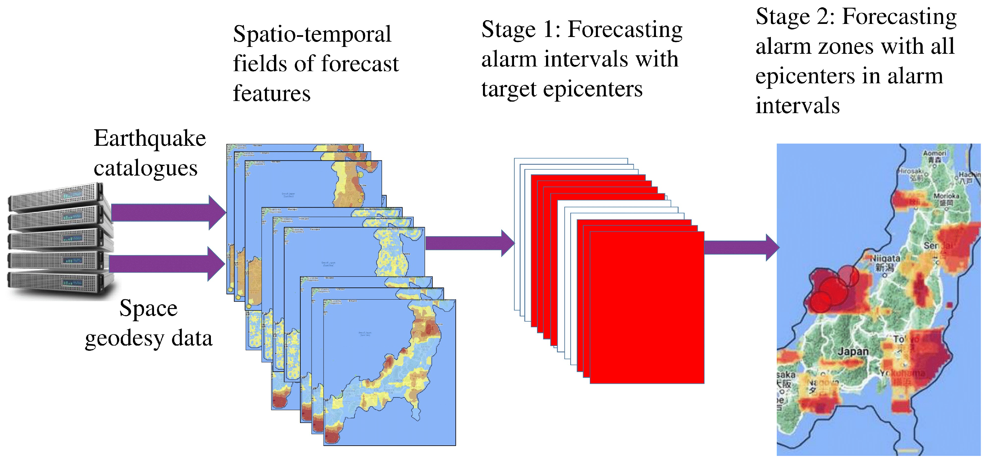
2.3. Forecast Scheme

The updated MMAA framework incorporates two key performance metrics to assess earthquake prediction efficacy. The metrics rely on three core parameters:
M * : number of forecast intervals where all target earthquake epicenters are located within predefined alarm zones.
M : total number of forecast intervals containing at least one target earthquake epicenter in the monitored region.
N * : total number of forecast iterations (time intervals) performed.
1.
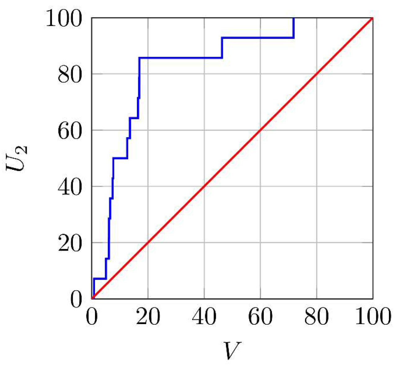
Detection probability:
U = M * M
The U indicator allows us to evaluate the quality of the learning algorithm and the information used for the forecast.
2.
Probability of a successful forecast in the next interval:
P = M * N *
The indicator P allows to estimate the effectiveness of the practical use of forecast results.
It follows from (2) that the estimate P depends on the number of intervals for which alarm zones are predicted. When the total number of forecast intervals N * is large and the number of intervals containing target earthquake epicenters M is small, the resulting probability P becomes too low for reliable decision making. To increase P , the number of forecast intervals N * must be reduced. This is achieved through a two-stage forecasting process, as illustrated in Figure 1. Before each forecast interval, input data (such as earthquake epicenters, time series, and raster fields) are retrieved from remote servers. These are used to calculate spatiotemporal grids of forecast features. In the first stage, the timing of target earthquakes in the analysis zone is predicted. If an earthquake is expected, the interval is marked as an alarm interval. In the second stage, specific alarm zones are identified within these N * intervals, indicating where target earthquake epicenters are likely to occur.
The purpose of the time-based forecast is to select as alarm intervals only those intervals that contain target earthquakes in the analysis zone. The purpose of the spatiotemporal forecast is to calculate area-limited alarm zones that contain all target earthquakes of the interval in the largest number of alarm intervals. The different purposes of the time and space forecasts are the reason for choosing different feature fields during training. In the time forecast, the most informative feature fields are those that have anomalous values only in intervals with target earthquakes. In the spatiotemporal forecast, the most informative are those that have anomalous values in zones where the epicenters of target earthquakes are expected.

2.4. Learning Algorithm

All available retrospective data are used for training, e.g., grid fields of features and epicenters of target earthquakes.
The first stage of training involves the transition from a set of the epicenters of target earthquakes to the training set of the vectors of the feature space. To achieve this, the method first calculates the possible precursors of target earthquakes and unmarked data. Possible precursors are spatial features corresponding to all nodes of the coordinate grid in the precursor cylinders with centers based on the epicenters of target earthquakes. The remaining nodes of the analysis zone grid correspond to unmarked records.
Now, for each possible precursor, the algorithm finds vectors that, according to the model, have properties (feature values) that are no less anomalous than the precursor itself. The set of these vectors forms an orthant, the vertex of which is the precursor. During training, each time slice of the feature fields produces new vectors in the feature space. This leads to the formation of new orthants and to changes in previously created orthants. According to the monotonicity condition, all orthant vectors can precede earthquakes similar to the one preceded by the precursor, which is the vertex of the orthant. However, the formal choice of precursors and the stochastic relationship of precursors with predicted earthquake epicenters indicate that, in reality, the prognostic capabilities of orthants differ. Therefore, the training algorithm selects the most informative orthants for the forecast.
At the next stage of training, the degree of informativeness of the orthants is assessed.
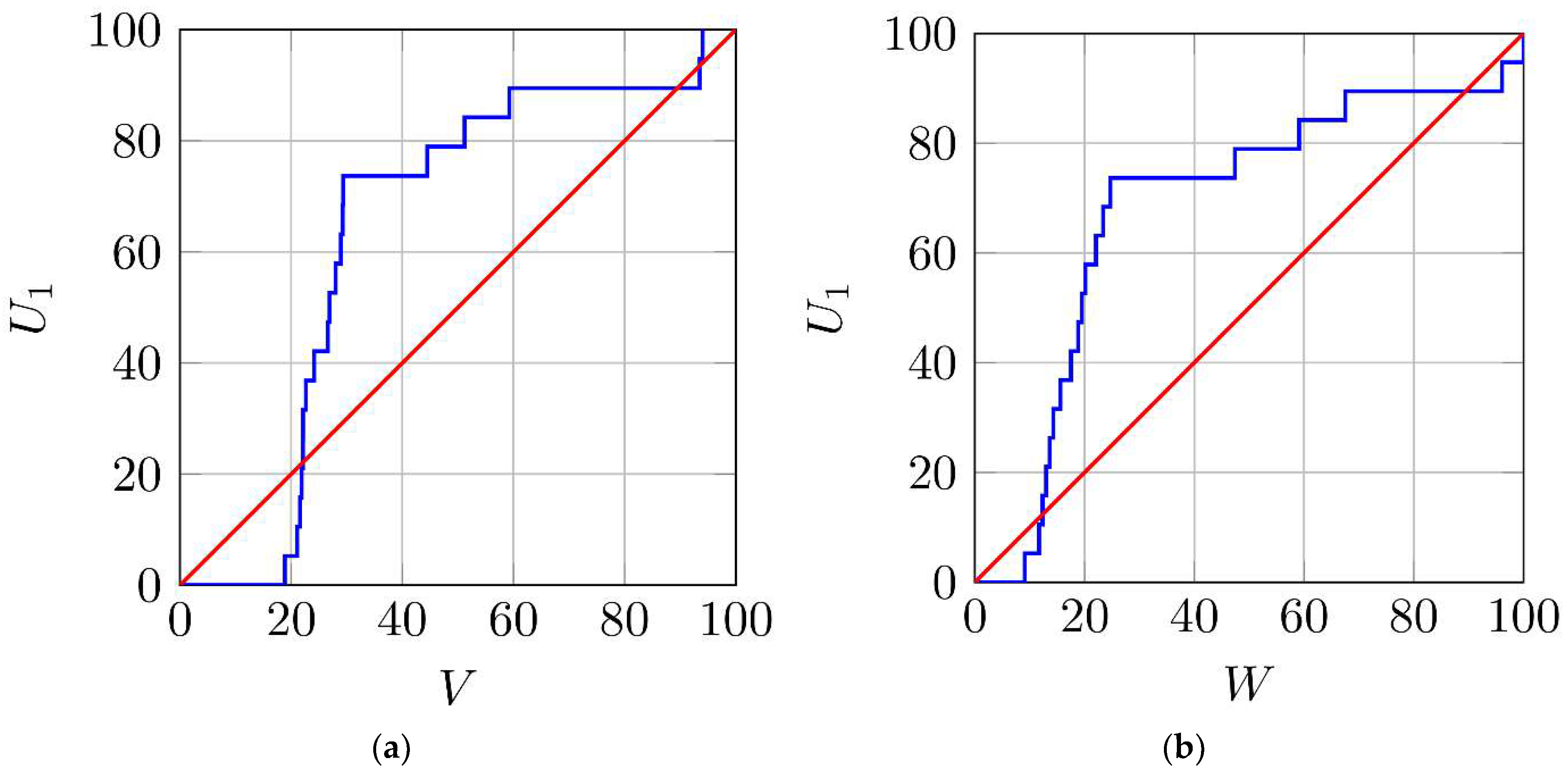
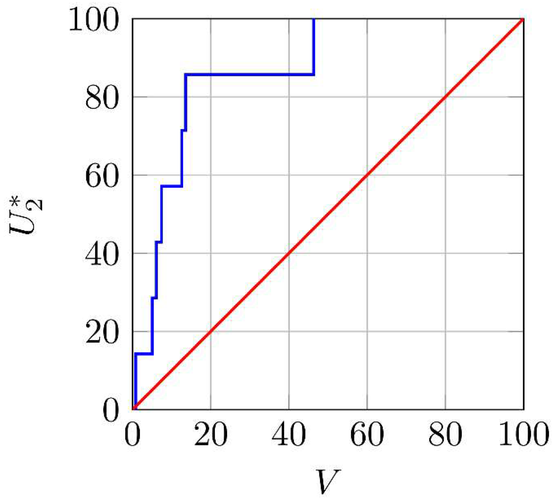
  • The measure of information content based on the alarm volume:
μ 1 ( n ) = 1 v ( n ) ,
v ( n ) = H ( n ) H ,
where v ( n ) is the alarm volume of the orthant h ( n ) . In time-based forecasting, H ( n ) is the set of prediction intervals corresponding to the vectors of the orthant, and H is the set of all prediction intervals. For spatiotemporal forecasting, H ( n ) is the set of grid nodes corresponding to the vectors of the orthant, and H is the set of all grid nodes in the analysis zone in space–time coordinates. From (3), it can be seen that the information content of the orthant increases as the number of vectors belonging to it decreases. A reduction in the number of vectors in the orthant is an indication that some components of these vectors are approaching anomalous maximum or minimum values of the feature fields. Consequently, according to the anomaly condition formulated in the method’s model, the information content of the orthant is greater the higher the likelihood that its vectors may turn out to be precursors of target earthquakes.
2.
The measure of information content based on the likelihood ratio:
μ 2 ( n ) = p T n p A ( n ) ,
p T ( n ) = H T ( n ) H T , p A ( n ) = H A ( n ) H A ,
where p T ( n ) and p A ( n ) are estimates of the potential earthquake precursors and unlabeled vectors, respectively, in the orthant h ( n ) . In time-based forecasting, H T ( n ) is the set of alarm intervals of the orthant, and H T is the set of all alarm intervals. For spatiotemporal forecasting, H T ( n ) is the set of grid nodes corresponding to the precursors of the orthant, and H T is the set of all grid nodes in the analysis zone corresponding to all earthquake precursors. In this case, the learning algorithm divides the feature space vectors into two classes. The target class vectors are defined as corresponding to the grid nodes associated with the previous cylinders. In this case, the sample of unlabeled vectors consists of all nodes of the coordinate grid nodes on time slices that do not intersect with the previous cylinders. Note that the accuracy of estimate (5) decreases with the decreasing number of orthant vectors, since it directly depends on the accuracy of the probability estimate p T ( n ) , p A ( n ) .
Next, the orthants are sorted in descending order of their information content, and the learning algorithm computes the alarm volume function V ( f ) . The computation of the function begins by assigning a value of 1 to all vectors in the feature space.
Figure 2 illustrates three orthants, h a , h b , h c , with decreasing information content from (a) to (c). The algorithm begins by selecting orthant h a , which has the highest information content, and assigns its vectors a value equal to its alarm volume v ( a ) (Equation (4)). It then proceeds to orthant h ( b ) , which has the next highest information content among the remaining orthants. The vectors in the set difference h ( b ) \ h ( a ) are assigned a value equal to the alarm volume of the combined region h ( a ) h ( b ) . This process continues iteratively, selecting the next most informative orthant and updating the alarm volume accordingly.
Next, the alarm volume function V ( f ) is mapped to prediction intervals depending on the forecasting type, i.e., to time intervals t for time-based forecasting, and to grid nodes ( x , y ) across all time slices within the training intervals for spatiotemporal forecasting. In the time-based forecasting stage, the alarm volume V ( t ) for each time slice t is defined as the minimum alarm volume among all vectors corresponding to the grid nodes within that slice V ( f x , y , t ) :
V t = min x , y V ( f x , y , t ) .
The alarm volume function V f is computed over the entire training material:
V f = N * N ,
where, for time-based forecasting, N * is the number of intervals for which the alarm volume value is less than or equal to V f , and N is the total number of forecast intervals. For spatiotemporal forecasting, N * , is the average number of grid nodes where the alarm volume value is less than or equal to V f , and N is the total number of grid nodes in the analysis area in space–time coordinates. The ordering of orthants by information content ensures that the precursors with small alarm volume values have the most significant impact on the forecast quality.
At each iteration, a threshold value V for the alarm volume is selected to make a decision about designating a forecast interval as an alarm interval or determining the size of the alarm zone. The threshold can be chosen in advance based on qualitative forecast indicators or estimated at each iteration by minimizing the loss function. In particular, the threshold can be calculated from the condition of minimizing the sum of the probability of missing at least one earthquake epicenter in the alarm zone and the alarm volume value during training V . The seismic hazard forecast is given when the inequality V f V is satisfied. For time-based forecasting, the fulfillment of this inequality at time slice t determines the designation of the interval ( t ,   t + Δ t ) as an alarm interval. For spatiotemporal forecasting, the fulfillment of the inequality during the alarm interval ( t ,   t + Δ t ) determines the selection of grid nodes for the alarm zone. It is easy to show that Formula (2) is a Bayesian estimate of the posterior probability of a successful forecast, provided that the forecast is made on N * intervals for which the alarm volumes V V .
The algorithm of the MMAA during training determines that the vector f k can be a precursor to earthquakes, similar to an earthquake with the precursor f n , if the vector f k belongs to the orthant h n with its vertex at the precursor f n . This allows for a textual explanation of the alarm zone computed during training. Indeed, the training algorithm forms alarm zones from grid nodes that correspond to vectors from the union of orthants. A grid node k belongs to the alarm zone if the conjunction expressing the membership of the corresponding vector f k in the orthant h n is satisfied:
f k h n , i f i = 1 I ( f i k f i n ) .
Furthermore, the membership of all grid nodes in the alarm zone can be explained using the following implication: “IF (conjunction 1) OR (conjunction 2) OR… is satisfied, THEN this alarm zone is predicted”. Most grid nodes in the alarm zone belong to the same orthants. Therefore, the number of conjunctions in the explanation is small. Additionally, the alarm zone can be explained by presenting a list of similar earthquakes that participated in the training. Similar earthquakes are those with precursors that are the vertices of orthants containing vectors corresponding to the grid nodes of the alarm zone.

3. Modeling

3.1. Data

As an example, we consider the application of the considered method to the systematic forecast of shallow-focus earthquakes in Kamchatka. These earthquakes are predominantly of a strike–slip or reverse nature and are confined mainly to the upper part of the subduction zone. To illustrate the technology of systematic earthquake prediction, let us consider an example for the Kamchatka region. The prediction training technology presented in the article differs from the one described in [19] in that, for time prediction, the information content of orthants is evaluated using the likelihood ratio measure (5).
The prediction is based on data from the earthquake catalog of the “Geophysical Service of Russian Academy of Sciences”, Kamchatka Branch, available at http://sdis.emsd.ru/info/earthquakes/catalogue.php (accessed on 6 May 2025) [21]. Raster fields for the prediction are calculated using earthquake epicenters since 1986 that have magnitudes m 3.5 and hypocenter depths H 160 km, within a coordinate raster grid of x y t = 0.1 ° 0.75 ° 30 days. The target seismic events are characterized by magnitudes of at least m = 6.0 and hypocenter depths not exceeding 60 km. The analysis zone is selected within the polygon with coordinates 157–169° east longitude and 49–58° north latitude. The boundaries of the zone are determined by the condition of the presence of at least 300 earthquake epicenters in a circle with a radius of 100 km from 1986 to 1996. The epicenter of the Great Kamchatka Earthquake of 5 November 1952 with a magnitude of m = 9.0 and a hypocenter depth of H = 21.6 km is located in this zone.
Training began on 10 January 2001. Testing was performed from 13 January 2012 to 6 September 2024, with a 30-day interval. During the testing period, N = 154 predictions were made, and Q = 33 target earthquakes with epicenters within the analysis zone occurred, falling into M = 19 prediction intervals. The analysis zone and the test earthquake epicenters are shown in Figure 3.
Based on the training results, the most informative feature fields for prediction are S 1 , S 2 , and S 3 .
S 1 is a field computed using the adaptive weighted smoothing (AWS) method applied to field S, which, in turn, is calculated based on the RTL criterion [22,23]:
s ( x , y , t ) = C n E n 0.33 exp r n R 2 exp t n T 1 ( ε r n R ) 1 ( ε t n T )
where x ,   y ,   t are the 3D coordinates of a node; C is a normalization constant; 1 u is an indicator function defined as 1 u = 1 ,   u 0 0 ,   u 0 ; n is the index of the earthquake epicenter; E n is the energy of the n-th earthquake, calculated as E = 10 k , where k = 4 + 1.8 m ; for the estimation, earthquakes with magnitudes m 5.0 , r n [km] is the distance from the grid node to the n-th epicenter; t n [days] is the time interval from the grid node to the n-th epicenter satisfying ( t ε T ) t n t . The field parameters include R = 125 km and T = 100 days (time interval) as attenuation coefficients, ε = 2. The field is smoothed using the adaptive weight smoothing (AWS) method [24,25], which preserves boundaries between regions with locally constant values by adaptively weighting spatiotemporal data based on their statistical structure. AWS employs a contrast measure derived from the Kullback–Leibler distance [26] and has been generalized for seismic parameter estimation via marked point fields [27].
S 2 is a field computed using adaptive weight smoothing (AWS) applied to the b-value field. The b-value field is calculated using the maximum likelihood criterion with a sliding window of parameters R = 125 km and T = 365 days.
S * is a field generated by applying AWS to the earthquake epicenter density field. This density field is obtained from the earthquake catalog using an exponential kernel smoothing method, with a spatial radius of R = 50 km and a temporal decay constant of T = 100 days.
S 3 represents the temporal variation in the S * field, expressed through Student’s t-statistic. For each time t, the value of S3 is calculated as the ratio of the difference between the average AWS-smoothed densities s * ¯ t and s * ¯ t T 2 ), computed over two consecutive intervals, T 1 = 3000 days and T 2 = 121 days, to the estimated standard deviation σ ( s * ) of this difference:
s 3 ( t ) = ( s * ¯ t s * ¯ t T 2 ) / σ ( s * ) ,
where s * ¯ t is calculated based on the values of the field S * over the interval t T 2 , t , and s * ¯ t T 2 is calculated over the interval ( t T 2 T 1 , t T 2 ) .

3.2. One-Stage Forecasting

Let us consider a spatiotemporal forecast where alarm zones are computed at each interval. Based on the training results, the values of the field S 3 close to the maximum are selected for the forecast. The forecast based on these field values is considered successful if the processes of preparation of the source of target earthquakes are accompanied by anomalous increases in the density of epicenters. When training in spatiotemporal forecasting, a measure of the informativeness of ortants by the volume of anxiety is used (4). To search for potential earthquake precursors, a cylinder is used with a base center at the epicenter of the target earthquake, a radius R = 12 km, and a generatrix T = 90 days is used to search for possible earthquake precursors. The threshold value for the alarm volume during training is set in advance at V = 0.2 .
Table 1 presents data on the detection of Q = 33 epicenters of test earthquakes. In the column labeled “Alarm Volume”, each test epicenter corresponds to the alarm volume value at the grid node closest to the epicenter of the target earthquake. The alarm volume value, V, according to (8), determines the average size of this alarm zone relative to the area of the analysis zone during training. Training involves the appearance of new data on forecast intervals, e.g., new vectors of feature field values at grid nodes and new epicenters of target earthquakes. These data update the information content indicators of orthants and form new orthants. The sorting of orthants by their information content indicators changes, leading to a change in the alarm volume function based on feature space vectors. However, the alarm volume values obtained in previous forecast intervals and the success of the forecast remain unchanged. If the alarm volume value at the grid node closest to the epicenter of the target earthquake exceeds the threshold V = 0.2 , this node does not belong to the alarm zone, and a missed target earthquake error is recorded. The corresponding rows in the table are highlighted in bold.
Figure 4 presents two graphs that are analogs of ROC curves [28]. The first graph U 0 ( V ) shows the dependence of the probability estimate U 0 of successfully detecting   Q * target epicenters in the forecast alarm zone on the alarm volume V, where, similarly to (1):
U = Q * Q ,
where the alarm volume V according to (8) determines the ratio of the size of the alarm zone required to detect a given epicenter to the area of the analysis zone during training. The second graph shows the dependence U * ( V ) in percent, where U * is an estimate of the probability of successfully detecting all epicenters of target earthquakes in the forecast alarm zone (1).
Figure 4 represents each successful forecast as a vertical interval. The abscissa axis shows the alarm volume values predicted during training, while the ordinate axis displays the success results of the forecast at the predicted alarm volumes. From Table 1 and the graph, it can be seen that, during testing with an alarm volume threshold of V = 0.2 , the number of detected epicenters is Q * = 30 out of Q = 33 . In most studies on earthquake prediction, the quality of the solution is assessed using the probability of detection, which is equal to the ratio of the number of predicted target earthquakes to the total number of occurred earthquakes. In our case, this estimate is
U 0 = Q * Q = 30 33 = 0.91 .
We believe that a more effective measure of the quality of seismic hazard prediction is the probability of detection, equal to the proportion of prediction intervals in which all earthquake epicenters fall within the forecasted alarm zones, relative to the total number of prediction intervals. This measure is more appropriate for defining seismic hazard prediction and is less dependent on the presence of earthquake aftershocks. The dependence U * ( V ) shown in Figure 2 demonstrates that, at the same alarm volume threshold V = 0.2 , all earthquake epicenters are detected within the alarm zones on M * = 16 prediction intervals out of M = 19 . This corresponds to the probability of detection estimate for all earthquake epicenters occurring during the prediction intervals (1).
U * = M * M = 16 19 = 0.84 .
Given that N = 154 forecasts were made during testing, we obtain that the probability estimate that all epicenters of target earthquakes will fall within the alarm zone on the next prediction interval (2) is equal to:
P * = M * N = 16 154 = 0.1 .

3.3. Two-Stage Forecast from 19 January 2012

The goal of time prediction is to identify alarm intervals during which the epicenters of target earthquakes are expected within the analysis zone. The parameters of the alarm cylinder are a radius of R = 10 km and a generatrix of T = 60 days. For the forecast, the maximum values of the S 1 field and the minimum values of the S 2 field are used, as these are considered the most likely indicators of impending earthquakes. The selected fields describe the energy properties of the seismic process. The precursors of target earthquakes identified by the training algorithm show that, in many cases, target earthquakes are preceded by an anomalous increase in released seismic energy. This is consistent with the LNT model [1,3].
In the training on the time forecast, a version of the algorithm of the MMAA with a binary classification of objects is used in [27]. In this version, the training set of possible earthquake precursors, as before, consists of feature space vectors corresponding to all grid nodes of the precursor cylinders. The training set of the unlabeled vectors corresponds to all the grid nodes of the time slices in the analysis zone that do not intersect with the time slices containing the precursor cylinders. For time prediction, the measure of the informativeness of the orthant is defined as the likelihood ratio estimate (5).
Figure 5 shows the graphs of the dependencies U 1 V and U 1 W in percentages. Both graphs show the dependencies of the probability of successful detection of all earthquake epicenters in the forecast intervals on the alarm volume. The graphs differ in that, in the U * ( V ) dependency, the alarm volume V is calculated according to (8) based on the results from the beginning of training to the moment of the next forecast (in our case, this is the moment of the end of testing). The second graph represents the U * ( V ) dependency, in which the alarm volume W is calculated according to (8) but is based on the results from the beginning of testing to the end of testing.
During the modeling, the threshold value of the alarm volume V is selected based on the condition of the minimum sum of the probability of errors in missing at least one earthquake epicenter in the analysis zone and the value of the alarm volume during training V. During training on all N = 154 forecast intervals, the algorithm selects the threshold value of the alarm volume V = 0.294 . If the value of the alarm volume before the next forecast interval is less than or equal to the threshold V, then this interval is declared an alarm interval. From Figure 3, it is clear that for this threshold value on M 1 = 14 alarm intervals out of M = 19 in the analysis zone, the epicenters of target earthquakes are detected, which, according to (1), corresponds to the estimate of the probability of successful detection of alarm intervals
U 1 = M 1 M = 14 19 = 0.74 .
From the graph of the dependence U 1 ( W ) , it can be seen that the probability of successful detection of alarm intervals U 1 = 0.74 corresponds to the alarm volume value based on testing results W = 0.25. This means that, during testing on N = 154 intervals, N 1 = W N = 0.25 154 = 39 alarm intervals are selected. Hence, the probability estimate that, on the next alarm interval with an alarm volume V V = 0.294 , the epicenters of target earthquakes will appear in the analysis zone on the next alarm interval is:
P 1 = M 1 N 1 = 14 39 = 0.36 .
Let us now consider the second stage of the two-stage forecast. In this phase, the spatiotemporal prediction algorithm calculates alarm zones on all alarm intervals where target earthquake epicenters are anticipated. The forecast is based on the feature field S 3 , using a prediction cylinder with a radius of R = 12 km, a height (generatrix) of T = 90 days, and a training alarm volume threshold of V = 0.2 . As a result, the algorithm constructs M 1 = 14 alarm zones across N 1 = 39 alarm intervals, successfully encompassing all target earthquake epicenters.
Figure 6 presents the graph of the probability estimate for detecting earthquake epicenters within alarm zones as a function of the training alarm volume, denoted U 2 ( V ) . The graph shows that all epicenters are located within alarm zones during M 2 = 12 alarm intervals. Therefore, the estimated probability of successful detection is:
U 2 = M 2 M = 12 19 = 0.63 .
The estimated probability that all epicenters of target earthquakes will fall within the alarm zone during a future alarm interval with an alarm volume V V = 0.3 is given by:
P 2 = M 2 N 1 = 12 39 = 0.33 .

3.4. Two-Stage Forecast from 11 January 2018

During the modeling period from 9 January 2001 to 22 August 2024, 288 forecasts were made, and 53 target earthquakes occurred in the analysis zone, which fell within 31 forecast intervals. During the testing interval from 19 January 2012 to 22 August 2024, 154 forecasts were made, and 33 target earthquakes occurred in the analysis zone within 19 forecast intervals. At the same time, the minimum number of intervals with earthquake epicenters used for training was 12. The small training sample of intervals had target earthquakes P 1 and P 2 . To increase the training sample, let us consider testing from 11 January 2018. During this period, 81 forecasts were made, and 15 earthquakes occurred in the analysis zone within 10 intervals. At the same time, the minimum number of intervals with earthquakes used for training increased to 21. It is possible that increasing the volume of the training sample of forecast intervals with earthquake epicenters will allow for higher values of the probabilities of successful subsequent forecasts, which we will denote as P 1 * and P 2 * .
Let us consider the results of systematic earthquake forecasting modeling obtained during testing from 21 January 2018 to 6 September 2024 with a 30-day interval. The precursor cylinder has a radius of R = 12 km and a generatrix of T = 61 days. During the testing period, N = 81 forecasts are made, and Q = 15 target earthquakes with epicenters in the analysis zone occur, which fall into M = 10 forecast intervals. In the time-based forecast, the precursor cylinder has a radius of R = 10 km and a generatrix of T = 60 days.
Figure 7 shows the graphs of the dependencies of the probability of successful detection of all earthquake epicenters in the forecast intervals on the alarm volumes U 1 * ( V ) and U 1 * ( W ) in percentages, obtained during the time-based forecast.
During modeling, the threshold value of the alarm volume V is chosen based on the condition of minimizing the sum of the probability of missing at least one earthquake epicenter in the analysis zone and the alarm volume V during training. When training on all N * = 81 forecast intervals, the algorithm selects a threshold alarm volume of V = 0.294 . If the alarm volume value before the next forecast interval is less than or equal to the threshold V, this interval is declared an alarm interval. From Figure 7, it can be seen that, for this threshold value, on M 1 * = 7 alarm intervals out of M * = 10 , the epicenters of target earthquakes are detected in the analysis zone, which, according to (1), corresponds to the estimate of the probability of successful detection of alarm intervals:
U 1 * = M 1 * M = 7 10 = 0.7 .
From the graph of the dependence U 1 * ( W ) , it can be seen that the probability of successful detection of alarm intervals U 1 * = 0.7 corresponds to the value of the alarm volume based on testing results W = 0.173 . This means that, during testing on N * = 81 intervals, N 1 * = W N * = 0.173 · 81 = 14 alarm intervals are selected. Hence, the probability that, with a forecast alarm volume V V = 0.294 , the epicenters of target earthquakes will appear on the next alarm interval within the analysis zone is:
P 1 * = M 1 * N 1 * = 7 14 = 0.5 .
Let us now consider the results of testing the spatiotemporal forecast, obtained only on the N 1 * =14 alarm intervals selected during the time-based forecast, out of which N 2 * = 10 contain earthquake epicenters within the analysis zone. The precursor cylinder has a radius of R = 12 km and a generatrix of T = 90 days. In Figure 8, the graph of the dependence U 2 * ( V ) is shown. From the graph in Figure 6, it can be seen that, on M 2 * = 6 alarm intervals, all earthquake epicenters fall within the alarm zones. Hence, the estimate of the probability of successful detection is:
U 2 * = M 2 * M = 6 10 = 0.6 .
The estimate of the probability that, on the next alarm interval, all epicenters of target earthquakes will fall within the alarm zone at an alarm volume V V = 0.294 is:
P 2 * = M 2 * N 1 * = 6 14 = 0.43 .
The prediction results show that, for the one-stage forecasting, the probability estimate of successful earthquake detection (14) is equal to U * = 0.84 , and the probability estimate of successful next-interval prediction (15) is P * = 0.1 , which are practically the same as those reported in [19]. In the two-stage forecasting, the probability estimates of earthquake detection range from 0.6 to 0.74, lower than in the one-stage forecasting. At the same time, from (17), (19), (21), and (23), it is clear that, for a two-stage forecast, the estimates of the probabilities that at the next alarm interval all epicenters of expected earthquakes will be in the analysis zone and in the alarm zone have improved compared with [19] and range from 0.33 to 0.5. Such an improvement in the accuracy of forecasting can be due to the replacement of the measure of the information content of orthants by the volume of alarm (3) with the measure of the information content of orthants by the likelihood ratio (5). Nevertheless, the obtained probability estimates P 1 * and P 2 * are still too low for formal use.

4. Discussion

As demonstrated in Section 2 and Section 3, one way to bridge the gap between systematic earthquake prediction and practical application is to shift from a single-stage to a two-stage forecasting scheme. To achieve this, the MMAA is significantly modified. In its updated version, a successful prediction is no longer defined by the detection of individual earthquake epicenters but rather by the identification of all epicenters within a forecast interval. Furthermore, prediction quality is now evaluated not only by the probability of earthquake detection but also by the likelihood that all epicenters will fall within the forecasted alarm zone during a given interval.
The preparation phase of an earthquake is intrinsically linked to its occurrence. However, the complexity and nonlinearity of factors influencing seismic processes introduce stochasticity into the relationship between precursors and the eventual time/location of strong earthquakes. Implementing systematic earthquake prediction requires computational approaches, including machine learning methods. Key challenges in applying ML to seismology include the following:
  • Uncertainty in selecting earthquake precursors based on epicenters.
  • Limited training data for target magnitude earthquakes.
  • Incomplete and noisy data describing earthquake preparation processes.
  • Ambiguity in classifying target earthquakes by magnitude thresholds.
In Section 2, we address algorithmic inaccuracies by assessing the validity of identified precursors. This is achieved through a modified training algorithm that ranks orthants (spatiotemporal cells) by their predictive informativeness. This study introduces a new likelihood ratio-based metric for orthant evaluation. Modeling results (Section 3) confirm that this metric enhances the probability of successful earthquake prediction within subsequent alarm intervals.
Furthermore, Section 3 demonstrates that increasing the number of training examples improves prediction success rates. Our systematic forecasting approach relies exclusively on open-access data (e.g., seismic catalogs). However, defining target earthquakes by arbitrary magnitude thresholds introduces additional complexities. In this case, the learning algorithm must, based on the available data and past target earthquakes, find a decision rule that distinguishes earthquake preparation processes with magnitudes above the threshold m M from those with magnitudes below the threshold m < M .
As is known, in classification problems, there are usually objective reasons why objects of one class are similar to each other, while objects of different classes differ from one another. In our case, the method of class separation is not related to the physics of the seismic process. Therefore, the input data do not contain physical properties that determine interclass differences for earthquakes with magnitudes close to the threshold.
The second reason is that the currently available data on the magnitudes of strong earthquakes have absolute errors ranging from 0.1 to 0.3, and sometimes up to 0.5. It is doubtful that the prediction of magnitude based on data about the preparation process of strong earthquakes can be more accurate than its actual measurements.

5. Conclusions

This paper presents a computerized approach to systematic earthquake prediction. The approach is based on a nonparametric machine learning method designed to address one-class classification problems involving rare anomalous events, under the assumption of a monotonic relationship between the predicted value and the properties of the target class objects. The learning method accounts for the following three key characteristics of the problem:
  • The absence of a training set of earthquake precursors, which is replaced by a set of earthquake epicenters.
  • The anomalous nature of seismotectonic processes preceding major earthquakes.
  • The existence of a monotonic dependence between the degree of anomaly in the properties of earthquake preparation processes and the identified values of precursor features.
To enable the practical application of systematic earthquake forecasting, this paper proposes solutions to the following machine learning tasks:
  • Methods for the automatic identification of potential earthquake precursors, assessment of their quality, and ranking by informativeness.
  • Methods for optimizing new forecast quality metrics:
    Detection probability, defined as the proportion of forecast intervals during which all epicenters of target magnitude earthquakes fall within a confined alarm zone.
    Probability of detecting all epicenters of target earthquakes within the alarm zone during a forecast interval.
  • A method for two-stage systematic earthquake forecasting:
    Stage A: prediction of alarm intervals during which the epicenters of target earthquakes are expected within the analysis region (first stage of forecasting).
    Stage B: prediction of alarm zones within which all epicenters of target earthquakes are expected during the alarm intervals (second stage of forecasting).
  • Verbalization of the nonparametric decision rule using logical implication, enabling the interpretation of predictions in terms of the properties of the analyzed processes.

Supplementary Materials

The following supporting information can be downloaded at: https://www.mdpi.com/article/10.3390/geosciences15050170/s1.

Author Contributions

Conceptualization, V.G. and A.D.; methodology, V.G.; software, A.D.; validation, V.G. and A.D.; formal analysis, A.D.; investigation, V.G.; resources, A.D.; data curation, A.D.; writing—original draft preparation, V.G.; writing—review and editing, A.D.; visualization, A.D.; supervision, V.G.; project administration, V.G.; funding acquisition, A.D. All authors have read and agreed to the published version of the manuscript.

Funding

This research was funded by Ministry of Science and Higher Education of the Russian Federation, State Assignment number FFNU-2025-0032 “Research and Development of Methods and Network Technologies for the Analysis of Large Spatiotemporal Data for the Purpose of Multidisciplinary Analysis and Forecasting of Natural and Socio-Economic Processes”.

Data Availability Statement

We used the earthquake catalog (Supplementary Materials) of the Kamchatka Branch of the Geophysical Survey of the Russian Academy of Sciences, available at http://sdis.emsd.ru/info/earthquakes/catalogue.php [21]. Accessibility of the catalog was checked on 17 March 2025.

Conflicts of Interest

The authors declare no conflicts of interest. The funders had no role in the design of the study; in the collection, analyses, or interpretation of data; in the writing of the manuscript; or in the decision to publish the results.

Abbreviations

The following abbreviations are used in this manuscript:
MMAAMethod of the Minimum Area of Alarm
AWSAdaptive Weight Smoothing
RTLRegion–Time–Length
ROCReceiver-Operating Characteristic Curve
IPEInstitute of Physics of the Earth

References

  1. Myachkin, V.I.; Kostrov, B.V.; Shamina, O.G.; Sobolev, G.A. Fundamentals of physics of earthquake focus and precursors. In The Physics of Earthquake Focus; Nauka: Moscow, Russia, 1975; pp. 9–41. [Google Scholar]
  2. Sobolev, G. Principles of Earthquake Prediction; Nauka: Moscow, Russia, 1993; p. 313. Available online: https://bigenc.ru/b/osnovy-prognoza-zemletriase-f5d385 (accessed on 6 May 2025).
  3. Sobolev, G.A. Avalanche Unstable Fracturing Formation Model. Izv. Phys. Solid Earth 2019, 55, 138–151. [Google Scholar] [CrossRef]
  4. Zavyalov, A.D. Medium-Term Earthquake Forecast: Fundamentals, Methodology, Implementation; Nauka: Moscow, Russia, 2006. [Google Scholar]
  5. Kagan, Y.Y. Earthquakes: Models, Statistics, Testable Forecasts; John Wiley & Sons: Hoboken, NJ, USA, 2013. [Google Scholar]
  6. Shebalin, P.N.; Narteau, C.; Zechar, J.D.; Holschneider, M. Combining Earthquake Forecasts Using Differential Probability Gains. Earth Planets Space 2014, 66, 37. [Google Scholar] [CrossRef]
  7. Zhao, Y.; Lv, S.; Liu, P. Advances in Earthquake Prevention and Reduction Based on Machine Learning: A Scoping Review. IEEE Access 2024, 12, 143908–143929. [Google Scholar] [CrossRef]
  8. Mousavi, S.M.; Beroza, G.C. Machine Learning in Earthquake Seismology. Annu. Rev. Earth Planet. Sci. 2023, 51, 105–129. [Google Scholar] [CrossRef]
  9. Sobolev, G.; Ponomarev, A. Earthquake Physics and Precursors; Nauka: Moscow, Russia, 2003. [Google Scholar]
  10. Kanamori, H.; Brodsky, E.E. The Physics of Earthquakes. Rep. Prog. Phys. 2004, 67, 1429–1496. [Google Scholar] [CrossRef]
  11. Ommi, S.; Hashemi, M. Machine Learning Technique in the North Zagros Earthquake Prediction. Appl. Comput. Geosci. 2024, 22, 100163. [Google Scholar] [CrossRef]
  12. Ridzwan, N.S.M.; Yusoff, S.H.M. Machine Learning for Earthquake Prediction: A Review (2017–2021). Earth Sci. Inform. 2023, 16, 1133–1149. [Google Scholar] [CrossRef]
  13. Panakkat, A.; Adeli, H. Neural Network Models for Earthquake Magnitude Prediction Using Multiple Seismicity Indicators. Int. J. Neural Syst. 2007, 17, 13–33. [Google Scholar] [CrossRef]
  14. Rhoades, D.A. Mixture Models for Improved Earthquake Forecasting with Short-to-Medium Time Horizons. Bull. Seismol. Soc. Am. 2013, 103, 2203–2215. [Google Scholar] [CrossRef]
  15. Kail, R.; Burnaev, E.; Zaytsev, A. Recurrent Convolutional Neural Networks Help to Predict Location of Earthquakes. IEEE Geosci. Remote Sens. Lett. 2021, 19, 8019005. [Google Scholar] [CrossRef]
  16. Corbi, F.; Sandri, L.; Bedford, J.; Funiciello, F.; Brizzi, S.; Rosenau, M.; Lallemand, S. Machine Learning Can Predict the Timing and Size of Analog Earthquakes. Geophys. Res. Lett. 2019, 46, 1303–1311. [Google Scholar] [CrossRef]
  17. Mignan, A.; Broccardo, M. Neural Network Applications in Earthquake Prediction (1994–2019): Meta-Analytic and Statistical Insights on Their Limitations. Seismol. Res. Lett. 2020, 91, 2330–2342. [Google Scholar] [CrossRef]
  18. Gitis, V.; Derendyaev, A. A Technology for Seismogenic Process Monitoring and Systematic Earthquake Forecasting. Remote Sens. 2023, 15, 2171. [Google Scholar] [CrossRef]
  19. Gitis, V.G.; Derendyaev, A.B. Optimization of the Approach to Systematic Earthquake Forecasting. J. Commun. Technol. Electron. 2024, 69, 285–307. [Google Scholar] [CrossRef]
  20. Gitis, V.; Derendyaev, A.; Petrov, K. Analyzing the Performance of GPS Data for Earthquake Prediction. Remote Sens. 2021, 13, 1842. [Google Scholar] [CrossRef]
  21. Chebrov, D.; Tikhonov, S.; Droznin, D.; Droznina, S.; Matveenko, E.; Mityushkina, S.; Saltykov, V.; Senyukov, S.; Serafimova, Y.; Sergeev, V.; et al. Kamchatka seismic monitoring and Earthquake prediction system and its evolution. Main results of observations in 2016–2020. RJS 2021, 3, 28–49. [Google Scholar] [CrossRef]
  22. Sobolev, G.; Tyupkin, Y.S. Anomalies in the weak seismicity regime prior to Kamchatka strong earthquakes. Vulkanol. Seismol. 1996, 4, 64–74. [Google Scholar]
  23. Sobolev, G.; Tyupkin, Y.S. Effect of vibration on failure and acoustic emission in a fault zone model. Vulkanol. Seismol. 1998, 19, 829–836. [Google Scholar]
  24. Polzehl, J.; Spokoiny, V.G. Adaptive Weights Smoothing with Applications to Image Restoration. J. R. Stat. Soc. Ser. B (Stat. Methodol.) 2000, 62, 335–354. [Google Scholar] [CrossRef]
  25. Polzehl, J.; Spokoiny, V. Propagation-Separation Approach for Local Likelihood Estimation. Probab. Theory Relat. Fields 2006, 135, 335–362. [Google Scholar] [CrossRef]
  26. Kullback, S. Information Theory and Statistics; Dover Publications: New York, NY, USA, 1997. [Google Scholar]
  27. Gitis, V.G.; Derendyaev, A.B.; Pirogov, S.A.; Spokoiny, V.G.; Yurkov, E. Earthquake Prediction Using the Fields Estimated by an Adaptive Algorithm. In Proceedings of the 7th International Conference on Web Intelligence, Mining and Semantics, Amantea, Italy, 19–22 June 2017; pp. 1–8. [Google Scholar]
  28. Fawcett, T. An Introduction to ROC Analysis. Pattern Recognit. Lett. 2006, 27, 861–874. [Google Scholar] [CrossRef]
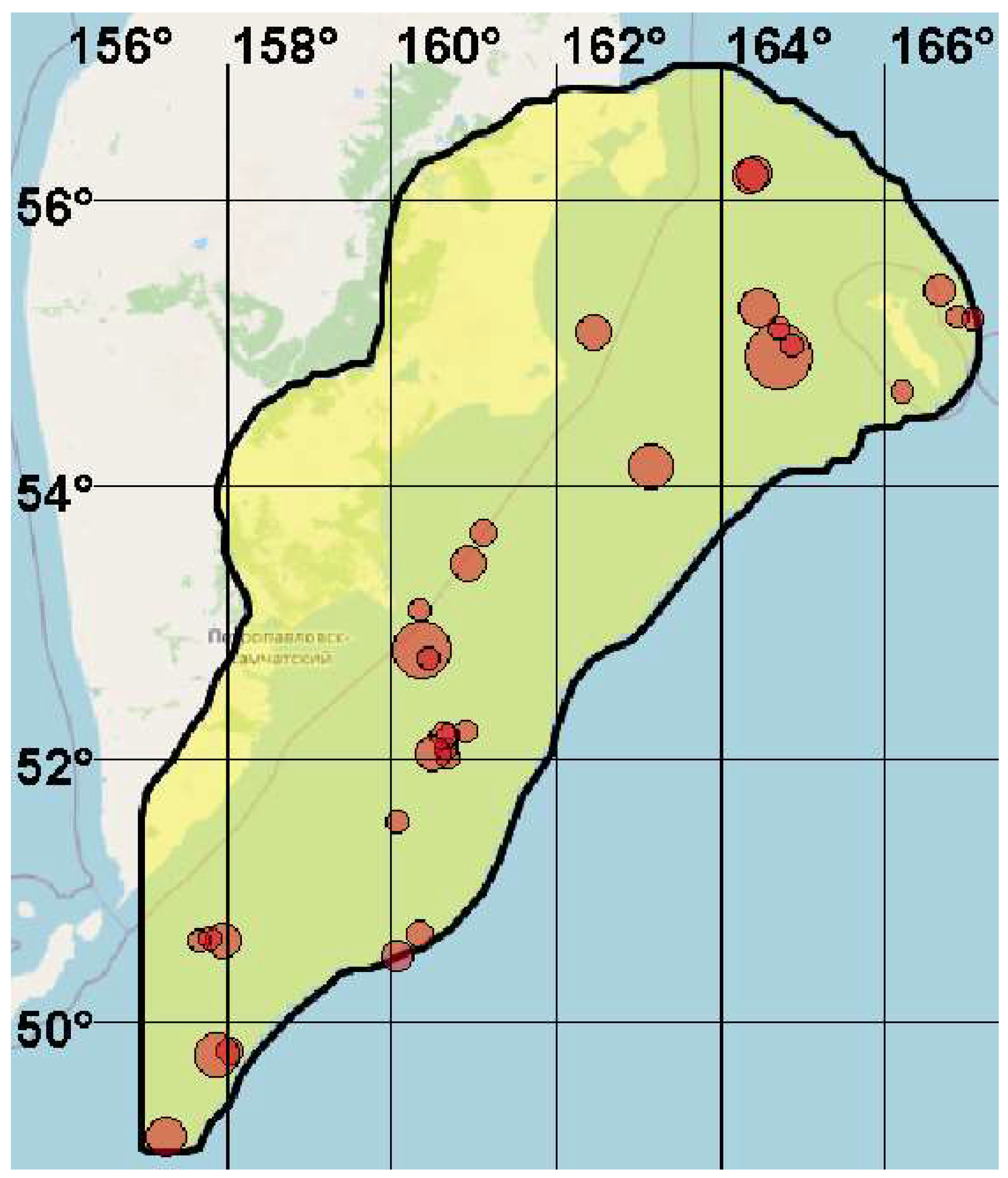
Figure 1. Block diagram of a two-stage systematic earthquake forecast.
Geosciences 15 00170 g001
Figure 2. Upper row: orthants h a , h b , h c , the information content of which decreases from (a) to (c). Lower row: the sequence of steps for calculating the alarm volume function V ( f ) .
Geosciences 15 00170 g002
Figure 3. Spatial distribution of earthquakes within the analysis zone from 13 January 2012 to 6 September 2024. Epicenters (red circles, scaled by magnitude) are shown for events with magnitudes m 6.0 and epicenter depths H 60 km.
Geosciences 15 00170 g003
Figure 4. Graphs of U 0 V (a) and U * ( V ) (b). The values of   U 0 , U * , and V are given as percentages. The blue curve represents experimental data; the red diagonal line corresponds to the random prediction baseline.
Geosciences 15 00170 g004
Figure 5. Graphs of dependencies U1(V) (a) and U1(W) (b). The values of U1, V, and W are given as percentages. The blue curve represents experimental data; the red diagonal line corresponds to the random prediction baseline.
Geosciences 15 00170 g005
Figure 6. Graphs of the dependency U 2 ( V ) . The values of U 2 and V are given in percentages. The blue curve represents experimental data; the red diagonal line corresponds to the random prediction baseline.
Geosciences 15 00170 g006
Figure 7. Graphs of dependencies U 1 * V (a) and U 1 * ( W ) (b). The values of U 1 * , V , and W are given as percentages. The blue curve represents experimental data; the red diagonal line corresponds to the random prediction baseline.
Geosciences 15 00170 g007
Figure 8. Graphs of the dependency U 2 * ( V ) . The values of U 2 * and V are given in percentages. The blue curve represents experimental data; the red diagonal line corresponds to the random prediction baseline.
Geosciences 15 00170 g008
Table 1. Spatiotemporal forecast of test earthquake epicenters.
DateLongitude, DegreesLatitude, Degrees Depth, kmMagnitudeAlarm Volume, %
115 October 2012160.0851.5344.06.016.94
21 March 2013157.9450.6352.06.416.44
34 March 2013157.6650.6351.06.116.44
49 March 2013157.8050.6549.06.16.55
524 March 2013160.3350.6858.06.26.55
619 April 2013158.0449.7745.06.26.13
720 April 2013157.8849.7439.06.76.13
819 May 2013160.6952.0150.06.18.07
919 May 2013160.6552.0842.06.08.50
1019 May 2013160.6752.1840.06.09.63
1121 May 2013160.8952.2259.06.116.90
1221 May 2013160.6352.1843.06.29.63
1321 May 2013160.4952.0548.06.57.69
143 July 2014166.8655.1943.06.07.67
153 July 2014167.0655.1840.06.07.34
1620 March 2016163.1454.1442.06.717.78
1714 April 2016161.1153.6648.06.210.30
1829 September 2017160.3353.1051.06.071.77
1925 January 2018166.6555.3746.06.35.06
2023 May 2018162.4455.0856.06.47.42
2110 October 2018157.2649.0941.06.676.43
2220 December 2018164.7154.9154.07.35.49
2320 December 2018164.8554.9954.06.05.49
2422 December 2018164.7155.1255.06.05.49
2524 December 2018164.4655.2551.06.67.21
2628 March 2019160.0750.5149.06.346.34
2725 June 2019164.4156.1857.06.40.82
2826 June 2019164.3656.1653.06.50.82
299 August 2019162.0455.7860.06.06.10
3020 February 2020160.9253.4452.06.412.60
314 April 2020166.2154.6737.06.013.59
322024 August 17160.3752.8146.07.16.37
3321 August 2024160.4552.7540.06.16.37
Disclaimer/Publisher’s Note: The statements, opinions and data contained in all publications are solely those of the individual author(s) and contributor(s) and not of MDPI and/or the editor(s). MDPI and/or the editor(s) disclaim responsibility for any injury to people or property resulting from any ideas, methods, instructions or products referred to in the content.

