Long-Term and Interannual Changes in the Land Area of a Barrier Using Multiple Satellite Images

Abstract

The Waisanding Barrier (WSDB) in Taiwan faces problems with regard to beach erosion and land area (LA) reduction. Due to the small amount of data generated and insufficient time periods used, the results of previous studies are only local rather than long term in nature. This study used 207 satellite images over 20 years to explore long-term and interannual changes in the LA of the WSDB. We developed both a surface fitting method (SFM) and a two-step interpolation method (TSIM) to reliably determine the LA of each image. When the tidal level of WSDB at the image acquisition is within ±0.25 m of the zero-meter shoreline, the LA obtained via the TSIM is similar to that of the SFM, while the other ones are quite different. The long-term decaying rate of the WSDB’s LA determined via both methods is about −0.40 × 10⁶ m²/year. The consistent differences in LA obtained from LiDAR and image data and the interannual variation in excess area (EA) are discussed, and the causes of these differences are land subsidence (LS) in the WSDB and excess wave energy (AEWE).

1. Introduction

Barrier islands not only offer ecological resources but also protect coastal ecosystems from storm damage [1,2]. The WSDB is a typical sandy barrier island on the west coast of Taiwan. In recent decades, the WSDB has faced problems with beach erosion and land area reduction due to external forces and reduced sand sources [3]. Some researchers have used satellite imagery, LiDAR measurements, or in situ topographic survey data collected over several years to analyze the shoreline changes in the WSDB under a research plan proposed by relevant units in Taiwan [3,4,5,6]. It is difficult to fully understand the WSDB’s decadal-scale morphological changes due to limited measurement periods. Chang et al. [7] used 13 LiDAR measurements over an 18-year period to investigate the decadal-scale morphological change in the WSDB. Traditionally, the collection of traditional shoreline datasets from on-site or LiDAR measurements has often been expensive and constrained in time and/or space. Therefore, insufficient observation data over a long period of time makes it difficult to understand long-term interannual shoreline changes. This study aims to establish the long-term and interannual shoreline changes in the WSDB to provide a reference for future project planning and design to protect the WSDB from barrier erosion.

Regarding beach erosion or morphological changes in a barrier island, some researchers have used morphodynamics and established numerical models to simulate the characteristics of morphological changes under different external forces. Some morphodynamic models have been developed to understand morphodynamic changes over time, such as XBeach [8], CSHORE [9,10], or SBEACH [11]. However, 1D XBeach often overestimates infragravity waves. McCall et al. [12] mimicked the IG wave transformation of more complex depth-averaged 2DH models in directionally spread seas to adjust this overestimation. Recently, some studies further refined shoreline dynamics [13] and implemented one-dimensional deterministic, dynamic models [14,15,16], essential for understanding erosion, sedimentation, and morphological changes in coastal zones. For the morphological changes in barrier islands, the physics-based XBeach model was applied to investigate the effects of land cover and limited sediment supply on low-lying barrier island morphology under storm conditions. Extreme storms cause a short-duration overwash regime that responds to the morphological changes in a low-lying barrier [17]. High-fidelity, high-resolution two-way coupled numerical models for coastal erosion and flooding during storms have previously been applied to understand the formation of a barrier island breach, as well as the breach’s effects on the lagoonal circulation [18]. However, these deterministic and dynamic models are effective and efficient in forecasting storm-driven erosion and can improve our understanding of profile evolution under storm impacts. Both 1D and 2D morphological models require inputs of waves and water levels and high-resolution ground surface data. Uncertainties in these initial and boundary conditions propagate through the models and can contribute to additional error [19]. These models are not suitable for accurately simulating seasonal or interannual morphological changes, so long-term morphological trends are difficult to forecast.

Until recently, obtaining accurate shorelines over large geographic areas from high-resolution satellite imagery provided applicable shoreline mapping for analysis in further studies on shoreline evolution. Using image processing technology, satellite images can extract waterline features [20]. Comparing satellite-derived waterline positions, we can easily and visually understand the evolution of the waterline or the change in the shape of a barrier [21,22,23,24,25,26,27].

The waterline is commonly defined as the interface between the sea and either the beach or the shoreline at a specific tidal level. When using remote sensing imagery, the tidal levels vary depending on when the image was taken. Even if the beach does not change, the water line on the beach changes with the tidal level. Therefore, it is possible that a waterline is different from the zero-meter shoreline based on Mean Sea Level. The changes in the zero-meter shorelines must be known to accurately study the beach change over time. The original waterlines extracted from images taken at different water levels should be moved to a zero-meter shoreline [28]. Tide correction is required for waterline extraction from images to determine the shoreline location and accurately analyze shoreline evolution [29,30,31].

To achieve the aim of this study, it is necessary to explore long-term and interannual changes in the LA of the WSDB using multiple SPOT 5–7 high-resolution satellite images available from 2004 to 2021 [6]. The tide level at the time of image acquisition, required for LA calculation, is obtained using the MOI.18v1 tidal level model and the monthly average correction method. Waterline extraction is performed using the NDWI. Then, LA enclosed by the waterline is obtained. Two methods are proposed to determine the LA enclosed by the whole shoreline of the WSDB for each image.

2. Materials

2.1. Study Area

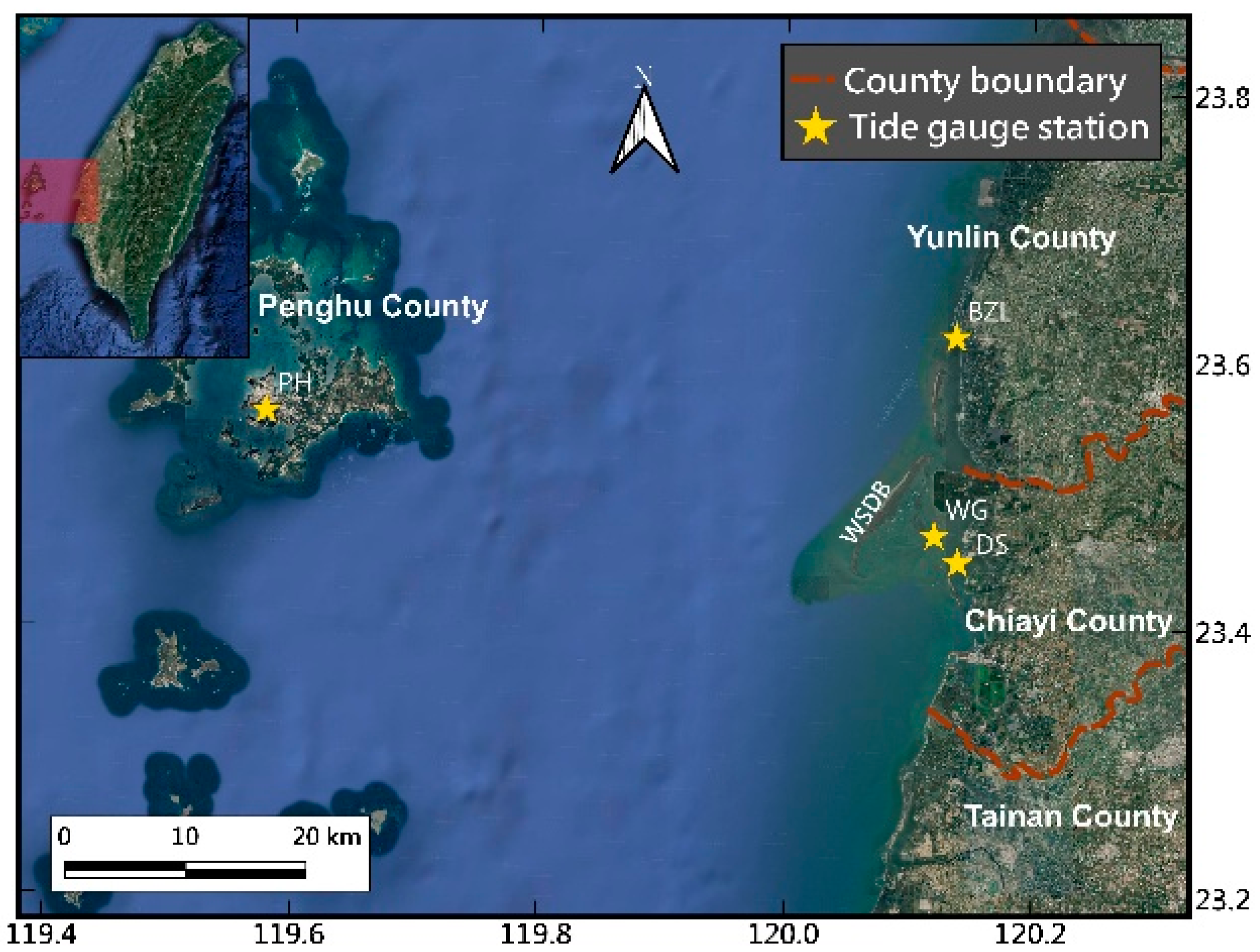
Figure 1 shows the location of the WSDB in Taiwan and four gauges on the Google Earth map for 2024. The WSDB extends away from the western coast of central Taiwan, which aligns subparallel to Taiwan’s west coast. It extends 12.6 km, and its land area is approximately 12.5 square km at low tide, which is about −1.2 m relative to the Mean Sea Level (MSL). The low-speed lagoon between the WSDB and Taiwan’s mainland serves as a major water area for oyster farming in Taiwan.

The WSDB is located in a shallow water area and does not have a tide gauge station. To correctly calculate the local tidal level at image acquisition, we required tidal level data from nearby tide gauge stations. Four tide stations near the WSDB provided reference tidal level data for the WSDB. The four stations are Boziliao (BZL), Dongshi (DS), Wengang (WG), and Penghu (PH), which are in Yunlin County, Chiayi County, and Penghu County, respectively.

2.2. Tides

Table 1. The statistics of the tides of four stations around WSDB, using a meter as the unit of measurement.

Station	MHW	MSL	MLW	MTR
BZL	1.451	0.233	−0.962	2.413
DS	1.198	0.337	−0.575	1.773
WG	1.016	0.116	−0.839	1.855
PH	1.142	0.002	−1.121	2.163

displays the tide statistics at each station based on analyzing tidal level data from the Central Weather Administration (CWA) in Taiwan spanning over ten years up to last year. The tidal level was based on the Taiwan vertical datum of 2001 (TWVD2001), which is the Mean Tidal Level at Keelung from 2002 to 2023 obtained by the CWA.

The statistics of tides included Mean High Water (MHW), Mean Sea Level (MSL), and Mean Low Water (MLW). These definitions are referred to in the report [32]. The Mean Tidal Range (MTR) was calculated as the difference between MHW and MLW.

The differences between the MHW and MSL at the four stations, as shown in Table 2, were 1.218 m, 0.861 m, 0.90 m, and 1.140 m, respectively. Furthermore, the differences between MSL and LLW at the four stations were 1.195 m, 0.912 m, 0.955 m, and 1.123 m, respectively. The MTRs of the BZL, DS, WG, and PH gauges were 2.413 m, 1.773 m, 1.855 m, and 2.163 m, respectively. Topography and water depth greatly influenced the tidal level in shallow water areas, as evidenced by the MTR difference of up to 0.64 m among three gauges. BZL is located at a higher latitude and in shallow waters, achieving the largest MTR. BZL, DS, and WG had MSLs of 0.233 m, 0.337 m, and 0.116 m, respectively, higher than that of PH. Because the positions of DS and WG were close, the difference in the MTR was only 0.082 m, but the difference in the MSL was 0.221 m.

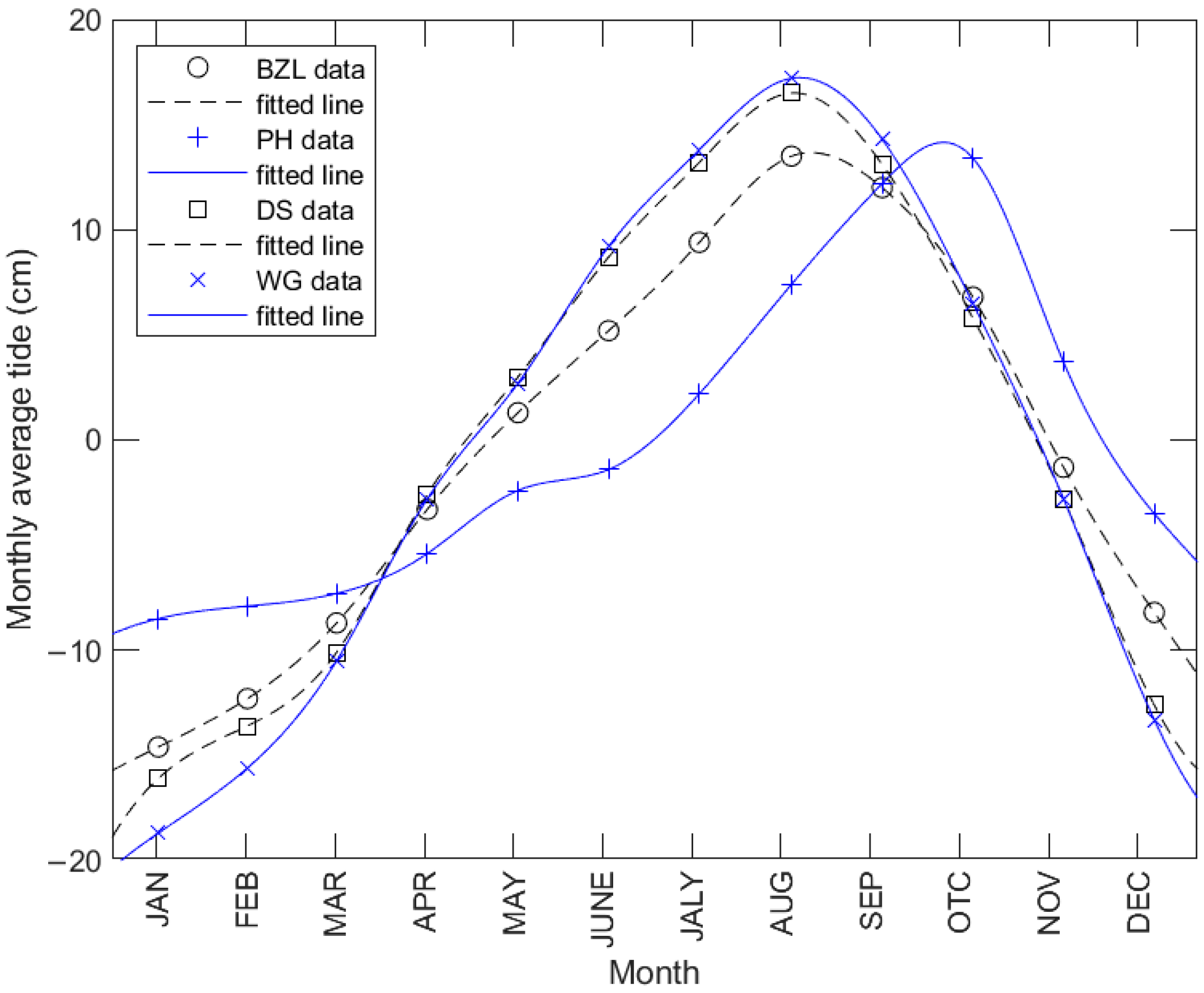
Synoptic water level conditions, which include tide, wave setup, monthly Mean Sea Level anomalies, and any remaining/residual bias, should be considered in determining the satellite-derived shoreline position [31]. Therefore, we obtained the monthly average tidal level data of these four tide stations from the webpage of the CWA, as shown in the four symbols in Figure 2 and their corresponding hourly smoothing curves.

The monthly average tidal levels at the BZL, DS, and WG stations were high in summer and low in winter, with the maximum value achieved in August. Since DS and WG are located close to each other, the changes in monthly average tidal levels were similar. BZL had a slightly lower maximum monthly average tidal level than both DS and WG. PH had a maximum monthly average tidal level in October and a minimum level in January. The variation in the monthly average tidal level at PH was different from that at the other three stations. The difference between the maximum and minimum values of PH was also lower than that of the other three stations. This may have been due to PH being located in the Taiwan Strait, with relatively deep and wide waters, while the other three stations are located in shallow waters. The latter three are greatly affected by water temperature.

2.3. Satellite Imagery

Launched in May 2002, the SPOT-5 satellite decommissioned its sensor on 31 March 2015. The panchromatic images captured by SPOT-5 are black and white with a 5 m resolution, but the super-mode panchromatic images, generated by combining two adjacent 5 m scenes, achieved a resolution of 2.5 m.

The SPOT-6 and -7 satellites launched in September 2012 and June 2014, respectively, and offer a continuity of optical imaging service up to 2024. The resolutions of the panchromatic and multispectral images taken by the SPOT-6 and -7 satellites were 1.5 m and 6 m, respectively.

A total of 207 clear images with limited clouds above the WSDB were collected from the SPOT-5 and SPOT-6 and -7 satellites from 2004 to 2021 through a research project. To comprehensively capture the temporal morphological changes in the WSDB, nearly all the available high-quality images were included to maximize the temporal coverage. The selection of SPOT-5, SPOT-6, and SPOT-7 imagery was based on their moderate spatial resolution, stable imaging quality, consistent time series, and good data availability for the study area, making them suitable sources for long-term coastal change analysis. The spatial resolution and the number of different satellite images used are summarized in Table 2.

In general, the spatial resolution of remote sensing images with both panchromatic and multispectral bands can be enhanced through pansharpening. However, after pansharpening, the SPOT-5 and SPOT-6/7 images still exhibited different resolutions, namely 2.5 m and 1.5 m, respectively. Considering that upsampling the lower-resolution SPOT-5 imagery could introduce artificial details without providing substantial benefits for waterline detection, the spatial resolution was unified by resampling the higher-resolution SPOT-6/7 imagery to 2.5 m. Subsequently, waterline extraction was performed using the NDWI, which enhances the contrast between land and water areas and delineates the wet–dry boundary (waterline) on the beach surface. A manual review was then conducted to integrate the 207 shoreline results, ensuring consistency and accuracy across the dataset.

Table 2. The spatial resolution and the number of different satellite images selected.

Satellite	Mode	Spatial Resolution (m)	Number of Selected Images
SPOT-5	Panchromatic	5	89
	Super-mode	2.5
	Multispectral	10
SPOT-6 and -7	Panchromatic	1.5	118
	Multispectral	6

Table 2. The spatial resolution and the number of different satellite images selected.

Satellite	Mode	Spatial Resolution (m)	Number of Selected Images
SPOT-5	Panchromatic	5	89
	Super-mode	2.5
	Multispectral	10
SPOT-6 and -7	Panchromatic	1.5	118
	Multispectral	6

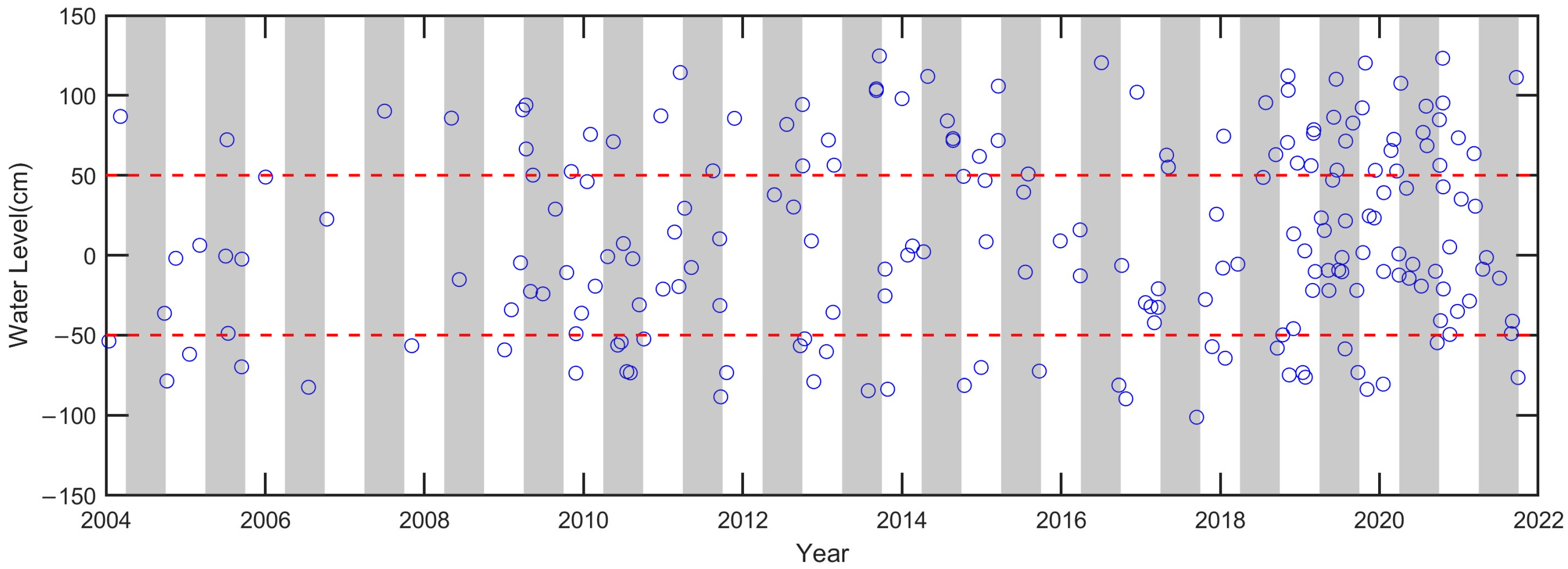
Figure 3 shows the time of image acquisition, denoted by a blue open circle and its corresponding tidal level. The two dashed lines in Figure 3 indicate the threshold of ±50 cm from zero tide, and the gray-shaded areas denote the summer season (April to September) to highlight the seasonal distribution of the images.

The figure shows that while relatively fewer images were collected during the early years, the number of available images in later years increased significantly. Regarding seasonal distribution, the images were collected throughout the entire year, without a strong bias toward any specific season. Therefore, the impact of seasonal variation on the overall shoreline change analysis was minimized.

3. Methods

3.1. Tidal Level Calculation

To correctly determine shoreline changes, the detected waterlines from images taken at different times needed to be corrected to the same tide reference, which is generally the Mean Tidal Level [28]. The correction required determining the local tidal level of the WSDB at image acquisition. The WSDB does not have a tide gauge station and is located in a shallow water area. Although the WSDB has some nearby tide stations and its distance is about 10 km, the tide data at these stations could not be directly used to estimate the local tidal level of the WSDB. Both the differences in the tidal level reference of each tide gauge station mentioned in Section 2.2 and the large phase differences in tidal levels due to spatial distance made it unreliable to estimate local tidal levels by directly using the tidal level data from a certain tide gauge station.

The Ministry of Interior (MOI) developed a regional tide model (MOI.18v1) to quickly calculate the tidal level for local waters around Taiwan. MOI.18v1 uses the MSL as the tidal level benchmark and considers 25 important tidal characteristics to quickly calculate the tidal level at a certain location and during a specified period. The root mean squared error (RMSE) between the observed and predicted hourly tides in the WSDB area for 2016 was approximately 10 cm. MOI.18v1, which has acceptable accuracy, is an applicable tide model in Taiwan. A detailed description of MOI.2018v can be found in the paper by Chang et al. [33].

Although semi-annual and annual tides are considered in the MOI.18v1 model, the amplitude of these long-period tides is small, and it is difficult to represent the significant seasonal differences in average tidal levels in shallow waters, as shown in Figure 2. To more accurately calculate the tidal level of the WSDB at the image acquisition time, we first calculated the tidal level at this time using MOI.18v1 and then added the average tidal level from the starting time of year shown in Figure 2. Therefore, we called it the monthly average correction method (MAC).

3.2. Waterline Detection

Chang et al. [6] used a five-step image processing method to obtain a black-and-white image for subsequent deep learning. The five techniques are as follows: (1) IHS fusion; (2) calculating the normalized difference water index (NDWI) to convert image information; (3) image enhancement; (4) image processing morphology for combination operations such as expansion or erosion; (5) binarization of land cover and sea cover markers.

After the above image processing, the land and water cover of the WSDB in the image were distinguished as a binarized image, and they were marked as 0 and 1, respectively. The boundary of the binarized image represented the waterline at the edge of the WSDB land area. The resulting binary image served as ground truth data, while the waterline position was used to calculate the WSDB area.

Chang et al. [6] created the SiamUnet architecture, which took different inputs from the top UNet to divide the WSDB into sea and land areas for all images. SiamUnet was examined to provide fast and accurate segmentation detection of the WSDB. The sum of the areas of all pixels detected as land in the image was the land area enclosed by the waterline of the WSDB, denoted as A_w.

3.3. LA Determination

When A_w is obtained from an image, two methods, the surface fitting method (SFM) and the two-step interpolation method (TSIM), are here proposed to determine A_s enclosed by the shoreline. Both methods are based on data interpolation. The SFM is a 2D interpolation, while the TSIM is a 1D interpolation. The following subsections introduce the algorithms of these two methods.

3.3.1. Surface Fitting Method

To accurately assess the change in the land area of a barrier, the calculated land area had to be based on the same tidal level, typically the tide datum, which is the zero-meter tidal level for coastal engineering in Taiwan. When the tidal level at image acquisition deviated from the 0 m tidal level, the position of the waterline extracted at such a tidal level differed from the zero-meter shoreline based on the tide datum. The calculated land area enclosed by the waterline had to be corrected to one enclosed by the shoreline. The geometric tangent principle could solve the problem of waterline-to-shoreline shifting when the beachface’s slope was known [28]. Since the slope of the beachface at the position of the whole waterline was not available, we proposed two methods to solve the problem.

A_w varied with the local tide, y (t), at time t and also underwent a long-term change, which was related to time. Therefore, A_w can be expressed as a function of both tidal level and time, as follows:

$$A_w=f(y\left(t\right),t)$$

(1)

When the data of the land area varied with the corresponding tidal level over a period of time, the function of Equation (1) could be approximately estimated via surface fitting. After the function was determined and the tidal level was set to zero at time t, Equation (1) yielded the land area at the zero-meter level, As. Cubic spline interpolation was employed to estimate the A_w of all images at different tidal levels. We utilized the fit function level in conjunction with the “cubicinterp” algorithm in MATLAB-R2024b to generate a surface that corresponded to 207 data points related to time and tidal level.

3.3.2. Two-Step Interpolation Method

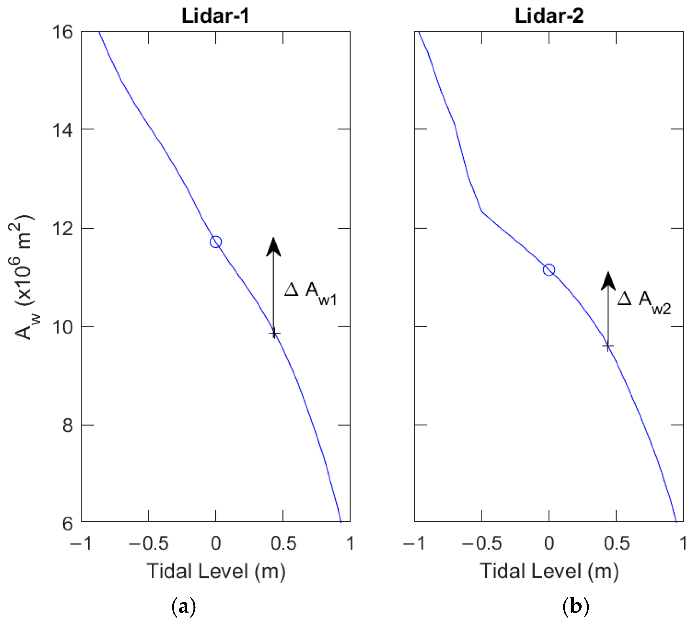
We used first-step data interpolation to adjust the two areas based on the tidal variation during the two LiDAR measurements. We calculated the land area from the digital elevation models (DEMs) of each LiDAR measurement enclosed by the waterline at an elevation level of −1.0 to 1.5 m per 0.1 m.

If a satellite image was taken between two adjacent LiDAR measurements, an example of the interpolated land area of the satellite image from these two LiDAR measurements is marked with a red asterisk at the blue curves in Figure 4a. We used the cubic spline interpolants to estimate the land area at the tidal level where the image was taken to be 0.439 m for the LiDAR-1 case, as shown in the left panel of Figure 4. The land area enclosed by the zero-meter tidal level is marked with a black circle, indicating the land area enclosed by the zero-meter shoreline at the time of such LiDAR measurement. The vertical line in the left panel of Figure 4, denoted by ΔA_w1, shows the area difference at such a tidal level and at the zero-meter level. Following the above procedure, we found the area difference, denoted by ΔA_w2, for another LiDAR measurement, as shown in the right panel of Figure 4.

The second step of the TSIM was conducting linear interpolation on time to find the area correction at satellite image acquisition, which was between the measurement times of the two LiDARs. The time differences between the image and two LiDAR measurements were denoted by Δt₁ and Δt₂, respectively. After finding ΔA_w1 and ΔA_w2, Figure 4 (b) shows the area correction at the time of the image. This can be shown via linear interpolation as

$$∆A_s=∆A_{w1}+{\displaystyle \frac{(∆A_{w2}-∆A_{w1})∆t_1}{∆t_1+∆t_2}}$$

(2)

Therefore, the land area at the zero-meter tidal level is equal to A_w plus ΔA_s; that is, A_s = A_w+ΔA_s.

To understand the differences between the two methods, the data requirement, algorithm, assumption, and application are listed in

Table 3. A summary table for data requirement, algorithm, assumption and application of both the SFM and TSIM.

Item	SFM	TSIM
Image data (Aw)	Yes	Yes
LiDAR data	No	Yes
Water level data (wl)	Yes	Yes
Algorithm	2D surface fitting	linear interpolation
assumption	No	$⌊wl⌋\le \pm 0.25\mathrm{m}$
application	High	Low

.

The SFM directly obtained the A_s of each image through a large amount of A_w and water level data. Because the SFM used cubic spline interpolation, the water level data covered the tidal range as much as possible. In addition, as the beach bed near the sea level can be considered as having a uniform slope, linear interpolation was considered feasible within this water level range. According to the analysis of this study, the ideal water level range was $⌊wl⌋\le \pm 0.25 \mathrm{m}$. From a methodological point of view, the TSIM assumed that AW changed linearly with the water level and required LIDAR data to be found. Therefore, the TSIM was less feasible than the SFM.

3.4. Index for Fit Performance

To determine the degree to which the model predictions approximated the real data points, a statistical measure was required. The coefficient of determination, denoted as R², is a common measure of the goodness-of-fit of a model [34]. R² is defined as follows:

$$R^2=1-{\displaystyle \frac{\sum _{i=1}^N{{[A}_m\left(t_i\right)-A_c\left(t_i\right)]}^2}{\sum _{i=1}^N{{[A}_m\left(t_i\right)-\overline{A_m}]}^2}}$$

(3)

where A_m (t_i) and A_c (t_i) are the observed and computed areas, respectively, at time t_i; $\overline{A_m}$ is the mean of A_m (t_i); and N is the total number of observed amplitudes. R² normally ranges from 0 to 1, indicating the proportion of the variation in the dependent variable that is predictable from the independent variable. Therefore, the higher the R², the closer the predicted value is to the measured value.

The alternative index, the root mean square error (RMSE), is frequently a good measure of the standard deviation of the residuals (prediction errors) for comparing the forecasting errors of different models. The definition of RMSE is

$$RMSE=\sqrt{{\displaystyle \frac{\sum _{i=1}^N{{[A}_m\left(t_i\right)-A_c\left(t_i\right)]}^2}{N}}}$$

(4)

Based on the definitions of RMSE, when the value is lower, the accuracy of the model prediction is higher, and, on the contrary, the larger the value, the worse the model’s predictive ability.

The linear correlation between two sets of sample data is commonly measured by a correlation coefficient (CC). The definition of CC is

$$CC={\displaystyle \frac{\sum _{i=1}^N{[A}_m\left(t_i\right)-\overline{A_m}\left]\right[ A_c\left(t_i\right)-\overline{A_c} ]}{\sqrt{\sum _{i=1}^N{{[A}_m\left(t_i\right)-\overline{A_m}]}^2}\sqrt{\sum _{i=1}^N{{[A}_c\left(t_i\right)-\overline{A_c}]}^2}}}$$

(5)

The correlation coefficient ranges from –1 to 1. A high absolute value of CC close to 1 implies that a linear equation describes the relationship between A_m (t_i) and A_c (t_i), with all data points extremely lying on a line. Zero CC implies that there is no linear dependency between A_m (t_i) and A_c (t_i).

4. Results

4.1. Assessment of Accuracy in Calculating Tidal Levels

Chang et al. [18] proposed a data fusion method (DF) and analyzed the degree of correction of the calculated tidal level via the MOI.18v1 model using the observed tidal level data of 22 tide stations in 2016. Therefore, the tide data of the four tide stations in 2016 are also used here to evaluate the accuracy of the proposed method for calculating the tidal level. The RMSE and correction percentage between the observed and computed tides at four tide stations using three methods is shown in

Table 4. RMSE and correction percentage between the observed and computed tides at the four tide stations using three methods, where the hyphen indicates data not evaluated.

Station	RMSE (cm)			Correction Percentage (%)
	HA	MOI.18v1	MAC	DF	MAC	DF
BZL	9.27	17.40	13.71	14.43	21.21	17.04
PH	8.32	14.18	12.03	11.23	13.33	20.81
DS	7.29	18.26	13.08	12.00	28.37	34.63
WG	7.87	18.62	10.55	-	43.34	-

. RMSE is the root mean squared error between the calculated tidal levels using various methods and the observed values at each station for 2016. The correction percentage is defined as the difference between the RMSE of the MAC or DF and the RMSE of MOI.18v1 divided by the RMSE of MOI.18v1.

In Table 4, it is shown that the HA has the lowest RMSE among the four methods, ranging from about 7.29 cm to 9.27 cm, and MOI.18v1 has the highest RMSE. The result of HA shows that in addition to the astronomical tide, which accounts for most of the tidal level in this water, there are minor parts, about 8 cm in length, affected by other secondary factors. The RMSE of MOI.18v1 is approximately twice that of the HA and can be reduced by 2.15 cm to 8.07 cm after correction via the MAC. The correction percentage determined via the MAC ranges from 13.33% to 43.34%. The station with the largest correction is WG. Using the DF, the reduction in the RMSE of MOI.18v1 is 2.07 cm to 6.26 cm, and the corresponding correction percentage is 17.04% to 34.63%. This result shows that the MAC’s correction to the tidal level calculated using MOI.18v1 is similar to that of the DF. However, the DF needs to estimate the tidal level data of more than three nearby tide stations at the same time, and it can only make hindsight-based corrections and cannot make future prediction corrections. The MAC does not have these limitations. Because BZL and PH are further from the WSDB than DS and WG and the MAC correction of WG’s tidal level is better than that of DS, the tidal level at the time of image shooting was first calculated based on MOI.18v1, and then WG’s MAC correction was applied.

4.2. Variation in Aw

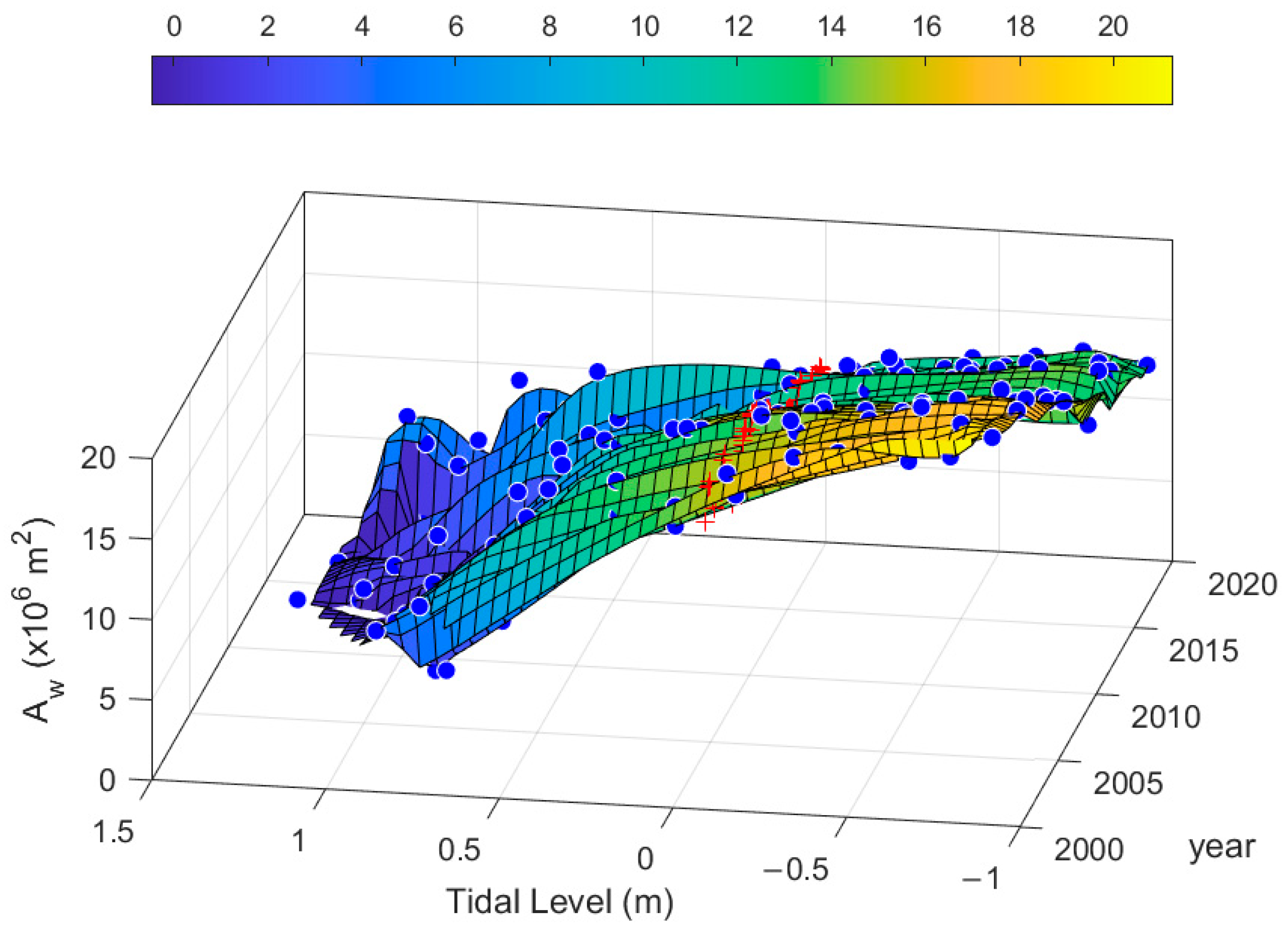
Figure 5 shows the fitted surface in the color bar and all images in blue circles with respect to two variables: tidal levels and years. The A_w reduction due to high tidal level and year-by-year changes is shown visually in Figure 5. By applying the zero-meter tidal level to the fitted surface, we can interpolate A_s from the time series. The red crosses in Figure 5 display the results of the SFM.

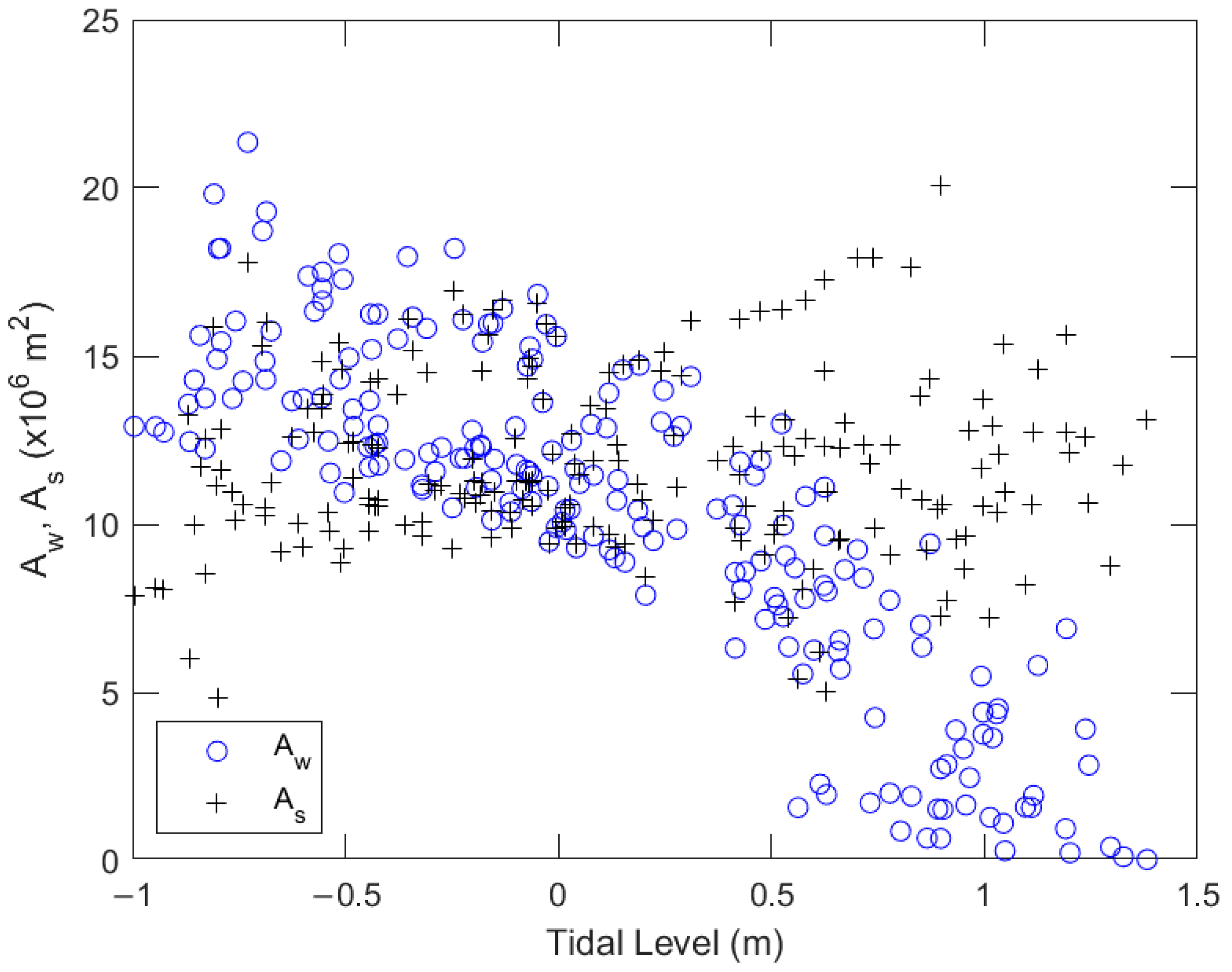
The waterline extracted from a satellite image is an instantaneous position at the moment when the sea water and the land intersect. The waterline’s position varies with the tidal level and changing beach. The blue open circles of Figure 6 show the A_w and A_s of the WSDB against corresponding tidal levels, which vary from about –0.91 m to 1.47 m. As the tidal level rises, the sea water submerges more land on the WSDB, leaving less land exposed. This leads to a reduction in the area enclosed by the waterline. The blue circles in Figure 6 show that the A_w of the WSDB has a quadratic and band-like attenuation as the tidal level increases. The value of CC between A_w and tidal levels is –0.8526, indicating a negatively strong relationship.

The red crosses in Figure 6 show the A_s made when the TSIM is used to fix the A_w that changes with the zero-meter tidal level. The A_s is spread out in a horizontal and band-like way. The CC between A_s and the tidal level is 0.0878, indicating that A_s is almost independent of the tidal level. Such a low correlation coefficient shows that the TSIM is suitable for correcting A_w due to the tidal level of A_s. However, when the tidal level deviates greatly from the zero-meter tidal level, the distribution range of A_s is larger than that when the tidal level is close to the zero-meter tidal level. This result is attributed to the large error caused by interpolation with a large deviation in the tidal level. On the contrary, A_w with a small tide level deviation is close to A_s, so the correction amount is small.

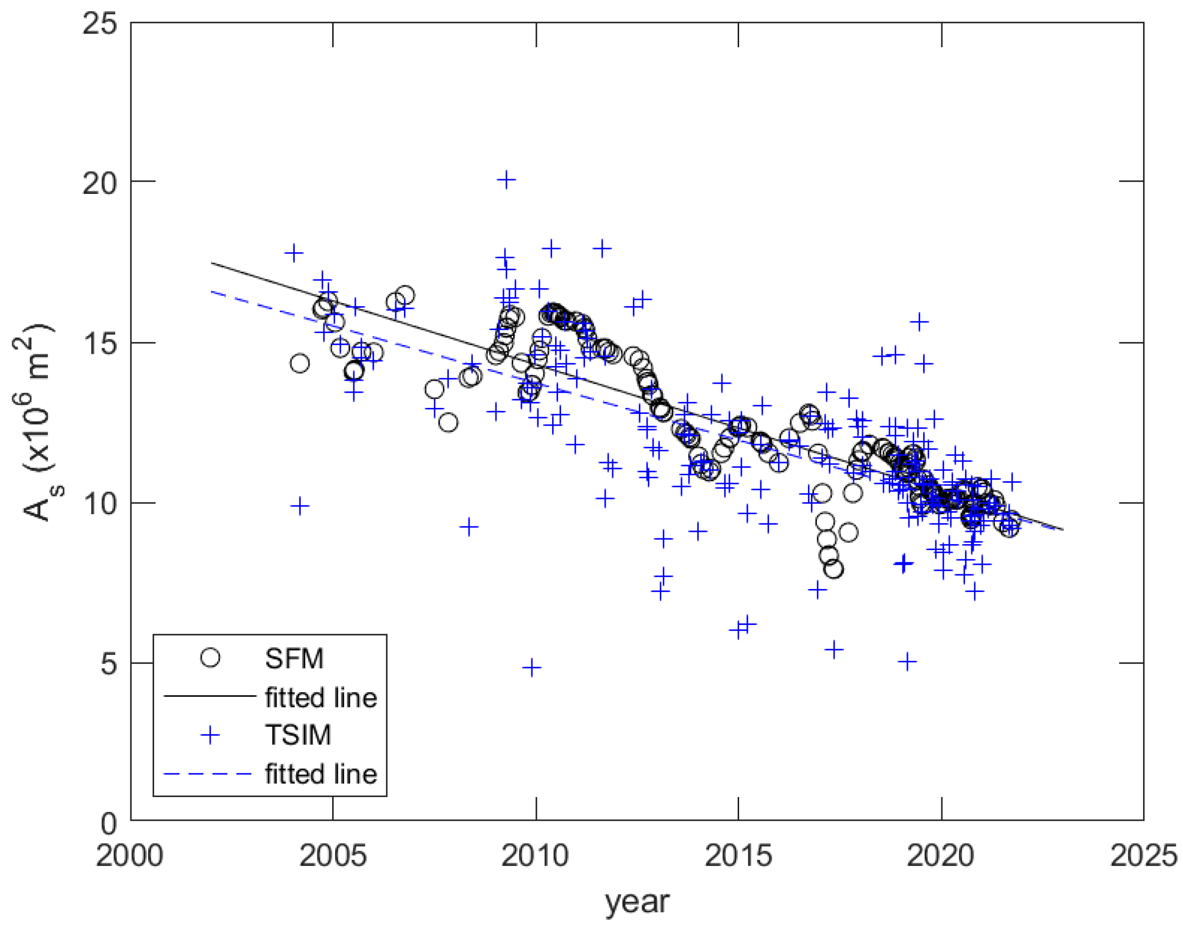
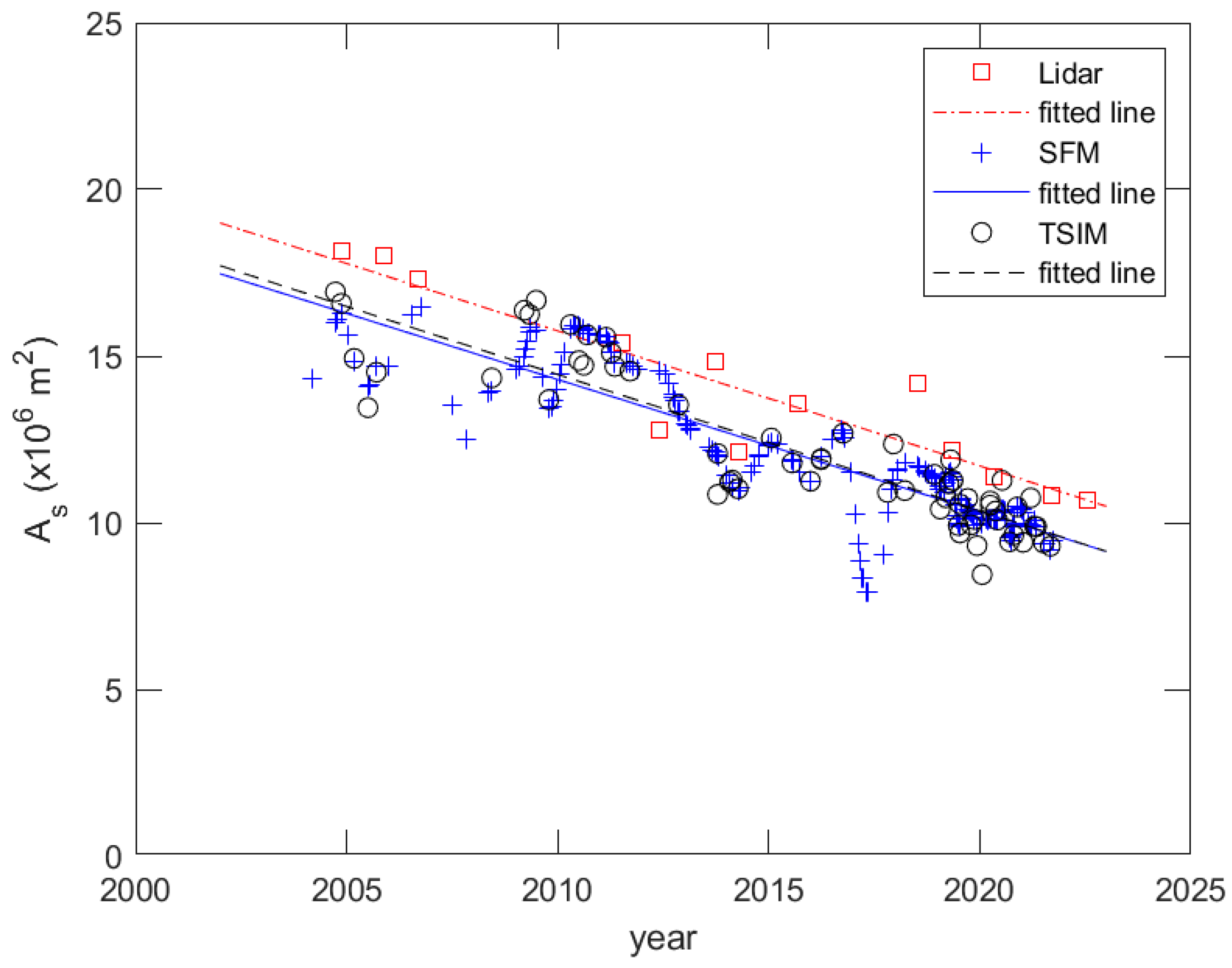
4.3. Long-Term Change in A_s

Regardless of the tidal level, both the TSIM and SFM can be used to determine A_s over time. Figure 7 displays the results for all images, with the open circles representing the areas obtained via the SFM and the crosses representing the TSIM. The two straight lines in Figure 7 are the fitted lines generated using linear regression for the two sets of A_s.

Figure 8 shows that the A_s estimated via the SFM is near the fitted line, but some A_s estimated via the TSIM deviates greatly from the fitted line. The deviation from the fitted line via the TSIM is much greater than that via the SFM.

The slope of both lines is –0.3568 × 10⁶ m²/year for data assessed via the TSIM and –0.3969 m²/year assessed via the SFM. For the TSIM, R² and RMSE are 0.4199 and 2.0279 × 10⁶ m². For the SFM, the values are 0.7795 and 1.0076 × 10⁶ m². The model accuracy evaluation shows that the error of the TSIM is about twice that of the SFM.

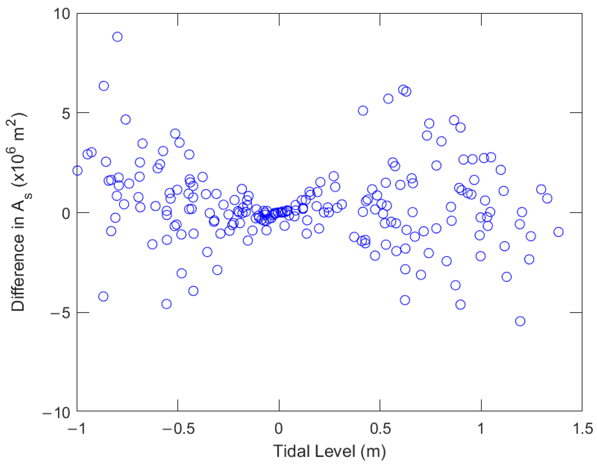
To investigate the short-term rapid change in the estimated A_s using the TSIM, in Figure 7, we show the difference in A_s estimated via the TSIM and SFM against the tidal level. Figure 8 shows that the area difference at a tidal level deviation higher than 0.25 m has a significantly large distribution. When the tidal level is in the range of $\pm$0.25 m, the estimated A_s is close. There are 63 such cases.

4.4. Validation of Results with the LiDAR Area

The LiDAR measurement method has been accepted by Taiwan’s authorities, and its DEM can be officially recognized as topographic mapping data. Due to the high cost of LiDAR measurements, only 13 measurements were taken from 2004 to 2022. Chang et al. [7] used LiDAR data to investigate the topographic change, beach orientation, land area, and volume of the WSDB. The estimated A_s values of 207 images determined via the SFM and those of 63 images determined via the TSIM at low tidal deviation are compared with those of the LiDAR data. The result is shown in Figure 9. Crosses, squares, and open circles represent the estimated A_s from LiDAR data and images assessed via the SFM and TSIM, respectively. The results of linear fitting for these data are represented by three straight lines: chained, solid, and dashed lines, respectively. The data from the SFM and TSIM are close, and the two corresponding fitted lines almost overlap. However, LiDAR’s estimated data exceed those of the SFM and TSIM. Therefore, the fitted line is roughly parallel and higher than the other two lines.

Table 5. The slope of the fitted line and the evaluation indexes for each data.

Method	Slope (×10 6 m2/year)	R2	RMSE (×10 6 m2)	MAD (×10 6 m2)
LiDAR	−0.4049	0.8551	0.9622	-
SFM	−0.3969	0.7795	1.0076	1.4386
TSIM	−0.4083	0.8072	1.0040	1.3165

summarizes the slope of the fitted line, representing the evaluation indexes for each data point, where MAD indicates the mean absolute difference between the predicted A_s determined via the TSIM or SFM and those of LiDAR data.

The slopes of these fitted lines, indicating the rate of area reduction, are very close, and they are –0.4049, –0.3969, and –0.4083 × 10⁶ m²/year, respectively. The R² of the prediction made using LiDAR data is 0.8551. For the SFM and TSIM, R² is 0.7795 and 0.8072, respectively. All three R² values are high. The RMSEs between the A_s obtained and the predictions determined using LiDAR data and images using the SFM and TSIM are 0.9622, 1.0076, and 1.0043 × 10⁶ m², respectively. According to these evaluation indicators, all three A_s values are close to the predicted values of time linear regression.

The A_s obtained via LiDAR data is calculated from the DEMs at a low tidal level, which is not affected by the tidal level, and can be used as the basis for the other two results. The last column in Table 5 indicates that the low offset of the SFM and TSIM deviating from the LiDAR data are 1.4386 × 10⁶ and 1.3165 × 10⁶ m², respectively. The difference in the MAD between the SFM and TSIM is about 1.221 × 10⁵ m², indicating that both A_s values are very close.

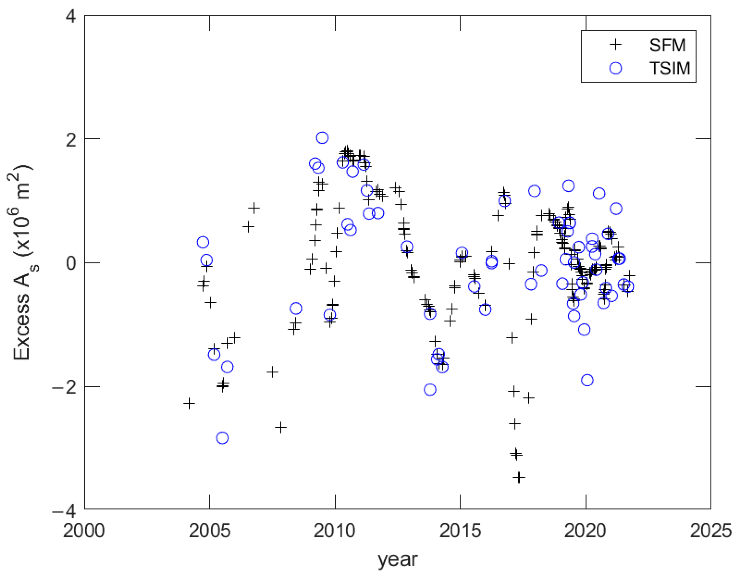
4.5. Interannual Excess Changes

The straight line in Figure 9 shows that in addition to the long-term area decrease, the WSDB also experiences interannual excess changes that deviate significantly from the straight line and are called the excess area (EA). Figure 10 shows the interannual change in the EA, in which the red crosses denote the results of the SFM and the blue open circles denote the 63 TSIM results.

Figure 10 shows that the changing trends of the two results are roughly consistent. Because of the later SPOT-6 and -7 satellites, the number of images in the later period is significantly larger than that in the early period. The EA was negative before 2009, turning positive until 2014 and becoming negative again from 2014 to 2018. The EA in the last five years was low. The result indicates that in addition to the quantitative decrease in the WSDB’s LA, there was also a decrease in the EA during 2004-2009 and 2014-2018. On the contrary, during 2009-2014, most of the EA increases.

If the waves are different in summer and winter, different profiles will be formed, which are called the summer profile and winter profile, respectively [35,36]. However, in Figure 10, the LA exhibits no seasonal changes. Perhaps this is because the number of images is not large enough to determine the time point when the beach advances or retreats. Another possibility is that the LA is a feature of the entire island and that it takes a storm wave to cause a dramatic morphological change, as well as that the degree of beach advance or retreat has little impact on the LA.

5. Discussion

5.1. Interannual Excess Changes

Figure 9 shows an issue worth discussing: an almost constant gap in the decrease in LA obtained from the LiDAR data and the images. The difference is about 1 × 10⁶ m². The variation in the LA in Figure 9 includes interannual changes and long-term decay. Chang et al. [7] investigated the morphological changes in the WSDB that are dominantly affected by LS and large waves induced by typhoons passing near the WSDB. Other influencing factors include sea level rise (SLR) and wind-driven sediments. The SLR at this area is much less than the LS [7]. Chang et al. [7] reasonably deduced that interannual changes in waves and winds are short-term effects of LA, and LS and SLR are long-term impact factors. If the WSDB has an LS problem, the height of the shoreline calculated from satellite imagery in the post-period will be higher than that in the pre-period, resulting in the shorelines in the pre- and post-periods not being on the same basis. LiDAR measures surface elevation and converts it to the elevation datum of TWVD2001. Therefore, the LiDAR data represent the actual elevation and are not affected by LS and, thus, need to be corrected.

The combination of LS and SLR can be estimated based on the annual average sea levels using tide data over a long period. The annual average sea level obtained via harmonic analysis from annual tide data may refer to that of Chang et al. [7]. The change rates of the annual average sea level for the BZL, WG, and DS stations are 32.03 ± 0.57 mm/year, 22.89 ± 0.87 mm/year, and 27.13 ± 0.68 mm/year, respectively. The average of these values is 27.35 mm/year [7].

Because the cost of an on-site geological survey is quite high, the WSDB’s geological compaction data have been unavailable until now for directly determining the LS rate. A possible estimate for the LS rate of the WSDB can be assumed to be 22.89 mm/year of WG or an average value of 27.35 mm/year. The WSDB is located between PH and WG. Assuming that the LS rate is linear, it is appropriate to interpolate the LS rate of PH and WG with distance to estimate the WSDB’s LS rate. The change rate of the annual average sea level at PH is 4.57 mm/year. The distance between PH and the WSDB is 58.72 km and that between WG and the WSDB is 8.50 km. The LS rate of the WSDB can be estimated via linear interpolation as 20.05 mm/year. If the LS rate is added to the tidal level of MAC, the evaluation index of LA change obtained via the SFM and TSIM is as shown in

Table 6. The slope of the fitted lines and the evaluation indexes for different LS rates.

Method	LS rate (mm/year)	Slope (×106 m2/year)	R2	RMSE (×106 m2)	MAD (×106 m2)
SFM	0.00	−0.4024	0.7795	1.0076	1.4386
	27.35	−0.3239	0.8600	0.6238	0.4873
	22.89	−0.3706	0.9122	0.5489	0.2433
	20.05	−0.3687	0.9155	0.5347	0.2015
TSIM	0.00	−0.3984	0.8072	1.0040	1.3165
	27.35	−0.2846	0.7217	0.9139	0.7086
	22.89	−0.3404	0.8055	0.8308	0.4606
	20.05	−0.35721	0.8475	0.7547	0.3028

. The TSIM still only uses data within ± 25 cm of the tidal level offset of 0 m.

Comparing the evaluation indicators of the SFM and TSIM under different LS rates, as shown in Table 6, the SFM has a higher R² and lower RMSE and MAD than the TSIM in each case. If we compare the four results of the SFM, the result that takes into account the LS rate will have better evaluation indicators than the one with a zero LS rate. For the LS rate of 20.05 mm/year, the evaluation result is the best among the three cases. Because there is no actual LS measurement from the WSDB, if the estimated LA obtained via LiDAR data is used as a reference, the MAD results in the last column of Table 6 show that the SFM method combined with the proposed tidal level estimate has the lowest MAD, which is 0.2015 × 10⁶ m², so the estimated LS rate of 20.05 mm/year is reasonable.

Considering this reasonable LS, A_s obtained via the SFM and TSIM under this condition is shown in Figure 11. If we compare Figure 9 and Figure 11, it is obvious that considering LS in tidal level estimation, the values of A_s obtained via the SFM and TSIM are very close to those of the LiDAR data. From a methodological point of view, more accurate tidal level estimation, that is, better data quality, can improve the estimation of the long-term trend of A_s.

Whether there is LS in the WSDB and its magnitude are all topics worth exploring in the future. However, since there are no local geological data for analysis or accurate estimates, using other methods to verify this LS estimate is also worthwhile for researchers interested in this topic.

5.2. Cause Analysis on EA

The datasets including LiDAR measurements used by Chang et al. [7] cover an 18-year period, which is similar to those of these images. However, the number of LiDAR measurements is only 13, far fewer than the number of the images, namely 207. It is easier to analyze the cause of the EA variation using these images than the LiDAR measurements.

In Figure 10, the EAs obtained via both the SFM and TSIM have a similar interannual variation in the WSDB. Since the SFM provides a denser dataset than the TSIM, it can fully present the variation characteristics of EA. For example, the TSIM lacks data in 2007 or 2017, as those years were insignificant. The EA reached high positive values during 2009–2013 but fell to low negative values in 2005, 2008, 2014, and 2017. EA does not exhibit evident regular seasonal changes every year, such as a decrease in winter and an increase in summer. There are strong northeasterly winds here in winter, and the corresponding waves are large, while in summer, the wind speed is slow, so the waves are also small [7]. These seasonal waves in winter and summer are not the main cause of EA changes. However, the typhoons that go through or pass by this area can induce huge waves larger than the winter waves for some days. These huge waves can overwash the sand on the whole land, and the dislodged surface sand will accumulate in the backbarrier. Chang et al. [7] used a 4 m threshold to compute their AEWE per year to relate to the significantly reduced land volume of LiDAR. The top four AEWE years are 2007, 2008, 2015, and 2016, and the years with low AEWE are 2009–2013. From this result, we can see that the change in EA is related to the excess accumulated energy of typhoon waves. For a more rigorous discussion, it is necessary to analyze the optimal threshold value with a higher correlation between AEWE and EA theoretically.

Recent numerical studies have simulated short-term topographic changes during storms [16,17,18]. If the relationship between representative values of external forces such as waves and the characteristics of topographic changes can be established, it can be applied to the analysis results of this study to clarify the relationship between LA changes and external forces.

6. Conclusions

Barrier islands are vital dynamic landforms that not only support ecological resources but also protect coastal ecosystems from storm damage. The WSDB in Taiwan has suffered from continuous beach erosion in recent decades. However, the interannual change in the WSDB’s LA cannot be explored due to insufficiently dense LiDAR data. We used 207 images and their water levels to develop two methods, the TSIM and SFM, for estimating the land area enclosed by the zero-meter shoreline and explore the long-term and interannual LA changes in the WSDB.

Since the WSDB lacks a tide gauge station to estimate the tide level of the image at that time, it can be used as the basis for correcting the A_w enclosed by the image waterline to A_s by the shoreline. The MOI.18v1 tide model associated with the monthly average correction method was developed to accurately calculate the tidal level of the WSDB at the image time. The A_w correction of the TSIM takes into account the deviation in the tide level from the zero-tide level. When the deviation is large, there will be a large error between the A_s corrected via the TSIM and that corrected via the SFM. It is shown that when the tidal level is in the range of $\pm$0.25 m, the A_s estimated via the TSIM is close to that estimated via the SFM. The A_s values estimated using the TSIM and SFM have a very similar long-term decay rate of –0.4 × 10⁶ m²/year, which is also consistent with that obtained from LiDAR data.

The difference in the decrease in LA obtained using LiDAR data and the images is constantly about 1 × 10⁶ m². With additional tidal correction based on the assumed LS rate of the WSDB, this difference is reduced. The equivalent LA of the WSDB obtained from two different data can indirectly infer the possibility that the WSDB currently is experiencing LS. This notion requires future geological exploration to provide direct evidence. The interannual change in the excess area of the WSDB was also analyzed to show increases or decreases in different periods. The cause analysis of the EA was proposed in this study, but its mechanism is three-dimensional and has long-term complexity. In the future, a physical model to simulate topological changes in the WSDB over a long period must be developed for comparison.