The geometry and context of the 11th SPE CSP (
https://spe.org/csp) is a synthetic geological cross-section with water-filled porous media, similar to the structures found in the Norwegian Continental Shelf. The model contains seven facies (rock types) to describe three versions of the CSP: Version 11A is a 2D experiment at laboratory scale and surface conditions. Version 11B is a 2D transect at field scale and conditions. Version C is a full synthetic field study as a 3D version of 11B. Their common 2D transect geometry with reasonable geological and operational realism is designed to keep problem statement simple and contain key computational challenges associated with numerical simulation of CO
2 injection, migration, and long-term storage [
18]. Some other considerations about the geology, fluid complexity, and petrophysical properties include the structural homogeneity for facies and faults, two-phase, two-component flow with thermal effects (pure water in the reservoir, with pure CO
2 injection) and the capillary forces and dispersion (for details, see [
18] and the CSP site mentioned above).
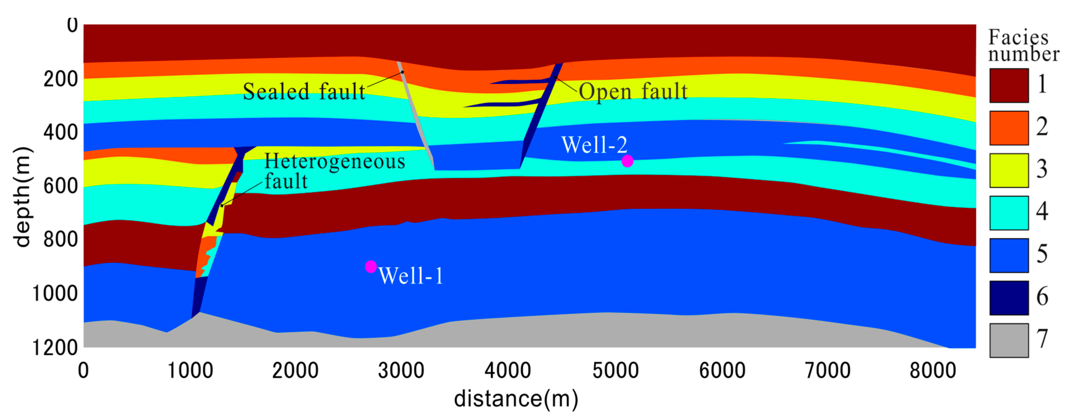
A sketch of the benchmark geometry of CSP 11B is given in
Figure 3 below. It is based on the description of the eclipse problem on the project site at
https://github.com/sintefmath/spe11-decks (accessed on 10 April 2025) (for other sketches, one can check [
18]). The coordinate system is oriented with the vertical direction pointing up and the origin in the lower-left corner. The dimensions of the cross-section are 8.4 km (horizontal) and 1.2 km (vertical). Moreover, a nominal depth of 1 m is assigned (to the y-direction) to be able to utilize volumetric expressions and units. The geometry includes seven internally homogeneous facies (six permeable and one impermeable), two injection wells (for pure CO
2), and three (almost vertical) fault-like structures with different permeabilities. The domain consists of the full porous medium except for the two injection wells. The boundaries are assumed impermeable. The figure contains two injection wells, which are specified in terms of their bottom left and top right corners, stated as (
x,
z) coordinates (measured relative to the lower left corner of the domain) with the coordinates (2700, 300) and (5100, 700).
2.1. Governing Equations and Constitutive Laws
The governing equations are adopted from the CSP 11 project description [
18], which is based on an isothermal two-phase, two-component version of Darcy’s law where constant model parameters and constitutive functions are used within each facies. For details, one can refer to [
18] and the references there, including [
19].
For the phases α = n (CO2-rich non-wetting gas phase) and α = w (H2O-rich wetting liquid phase), the main equations are summarized below:
The volumetric flux u
α of each phase
α is governed by the multi-phase Darcy’s law:
where
is the phase pressure,
and
k are the relative and intrinsic permeabilities, respectively,
is the phase viscosity,
is the phase density, and
g is the gravitational force pointing “down” with the approximate magnitude |
g| = 9.81 ms
−2.
Component mass conservation for components
i = CO
2 and
i = H
2O is as follows:
where
ϕ is the porosity,
is the component mass fraction in phase
α,
t is the time variable,
is the saturation,
J is a volumetric density term (i.e., reservoir volume per domain volume) for adding volume to boundaries, and
is the sum of diffusive and dispersive fluxes for component
i in phase
α given in Equation (3) below:
where
Dα is the mutual diffusivity in phase
α, while the term
E|
uα| is due to the assumption of linear dispersion in the model.
Capillary pressure: The phase pressures are related by saturation as follows:
Completeness of model: For phases
α =
n,
w and components
i = CO
2, H
2O,
Thermodynamics: The thermal equation for multi-phase flows in porous media (with the omission of kinetic energy) with the sum being over
(as in [
19]) is as follows:
where the solid phase is designated by
α =
s, and its saturation is set to
ϕ ss = 1 −
ϕ along with zero Darcy flux:
= 0. Moreover,
represents the internal energy per mass, and
is the thermal conductivity in Equation (6).
In addition to the governing equations, the following constitutive laws are considered.
Brooks–Corey type relative permeability and capillary pressure: For primary drainage (initial period of injected gas displacing water), saturations are normalized:
where
is the saturation below which the phase is immobile. The relative permeability is modeled as a nonlinear function of saturation:
(
) =
. If
is the basic Brooks–Corey capillary pressure, then an extended capillary pressure expression that is valid for all saturations with smooth transition to the maximum value,
, can be obtained using Equation (8) below that also involves the error function,
erf:
Thermodynamics: The thermodynamic properties for phase partitioning, pure-phase characteristics, and mixture properties follow those outlined in [
18]:
- (i)
The solubility limit of each phase (CO2 solubility limit in the water-rich wetting phase and H2O solubility limit in the CO2-rich non-wetting phase) is calculated based on the pressure of the same phase. Mass transfer between phases occurs instantaneously at each point, immediately dissolving or vaporizing available CO2 and H2O until the solubility limit is reached.
- (ii)
The pure-phase properties of CO
2 and H
2O and phase pressures are defined according to the NIST database [
20], available at
https://webbook.nist.gov/chemistry/fluid/, accessed on 10 April 2025. For the solid phase, the internal energy is a constant heat capacity, while for other phases, it is a function of both pressure and temperature.
- (iii)
Due to the very small mutual solubilities in this setup, all mixture properties are assumed to be equal to those of the pure phases, except for water density, which follows the form described in [
21]. Moreover, the rock is considered incompressible, and thus
ϕ does not vary over time.
Initial conditions: The CSP 11B model is initialized at t = −3.1536 × 10¹⁰ s (1000 years before injection begins). The initial conditions are given by considering an initially stagnant water-filled reservoir, the geothermal gradient, and a consistent pressure specification at the center of Well 1.
Boundary conditions: All the boundaries are impermeable (no-flow boundary conditions for the fluid): uα ⋅ n = 0 and jiα ⋅ n = 0, where n is the (outward) normal vector to the boundary. For the energy equation, an insulating boundary condition, n ⋅ ∇T = 0, is applied to the left and right boundaries, while a constant temperature is maintained at the top and bottom boundaries (based on the geothermal gradient and the depth z).
To prevent an unphysical increase in reservoir pressure, additional volume is introduced at the horizontal boundaries using a variant of pore volume multipliers. This approach typically involves assigning elevated volume content to cells at the domain boundary. The rigorous mathematical treatment is provided in [
18], utilizing a Dirac-type distribution on the boundary and describing volume per area at each boundary and within the corresponding facies. Additionally, the two injection wells (j = 1, 2) are equipped with fixed temperature boundary conditions during injection and zero heat transfer.
The material properties of the six permeable and one impermeable facies and model parameters (permeability, porosity, saturation, heat conductivity, diffusion constants, pressure, dispersivity, rock density etc.) closely follow the values given in Tables 4 and 5 of [
18]. However, the actual parameters used in the simulations are as in the problem sets of the CSP 11 research team of SINTEF:
https://github.com/sintefmath/spe11-decks, accessed on 10 April 2025. The full facies permeability is defined based on a 10:1 horizontal to vertical anisotropy ratio from the horizontal permeability. In addition, the capillary entry pressure is defined based on the Leverett J-scaling and a constant term reported by [
22] and also used in [
18].
2.2. Numerical and Computational Methods
Equations (1)–(6) form a system of coupled nonlinear partial differential equations (PDEs) of multi-phase and multi-component flow with thermal effects. Suitable numerical methods and discretizations including finite volume, finite difference, or finite element methods are employed to solve them approximately. These techniques ultimately transform the governing system of PDEs into linear algebraic systems that usually involve very large, sparse (populated with many zero entries), non-symmetric, indefinite, and ill-conditioned coefficient matrices. Such a large sparse linear system may not be solved via direct methods like Gaussian elimination or LU decomposition. However, it is possible to find robust and efficient approximate solutions via iterative linear solvers based on Krylov subspace methods, especially if the iterative solver is paired with a suitable preconditioner to address the ill-conditioned nature of the system [
10,
23]. A significant proportion of the overall computational time of reservoir simulations is used in the linear solver/preconditioner stage. Thus, selection of a computationally efficient method that produces accurate and stable results is of crucial importance in reservoir simulations. A list of linear solvers and their key properties are summarized in
Table 1. More details about these and other solvers are given below.
The classical conjugate gradient (CG) method and minimum residual (MINRES) algorithm apply only to symmetric matrices, but they have several extensions for more general linear systems including conjugate gradient squared (CGS), generalized conjugate residual, biconjugate gradient (BiCG), biconjugate gradient stabilized (BiCGSTAB), orthogonal minimum residual (ORTHOMIN), and generalized minimum residual (GMRES) methods, along with their variations such as restarted GMRES and loose GMRES (LGMRES), among others. Due to their flexibility, computational efficiency, and empirical convergence in reservoir simulations, GMRES, BiCGSTAB, and ORTHOMIN are preferred as linear solvers, often being used in conjunction with appropriate preconditioning and relaxation methods [
10,
23,
24,
25,
26]. There is no fixed combination of a linear solver and preconditioner pair that works best in terms of both computational efficiency and accuracy/convergence properties for all types of nonlinear problems. Moreover, there is no general convergence theory for a number of Krylov subspace methods that are designed for non-symmetric indefinite systems, including BiCGSTAB and restarted GMRES. So, an effective choice for a solver/preconditioner pair depends on the type and complexity of the problem, constraints, and method of discretization [
10,
15]. It is noteworthy that another robust and efficient method for approximating solutions to some non-symmetric large linear systems is induced dimension reduction (IDR), though it has not yet become a popular choice in reservoir simulations.
As previously mentioned, the most commonly used linear solvers in reservoir simulations are GMRES and BiCGSTAB. These methods, along with their various variants, offer distinct advantages depending on the specific characteristics of the simulation. Each solver has scenarios where it can outperform the other, as demonstrated by examples in the literature [
10]. A thorough mathematical analysis of both GMRES and BiCGSTAB, including their underlying principles and performance considerations, can be found in works such as [
24,
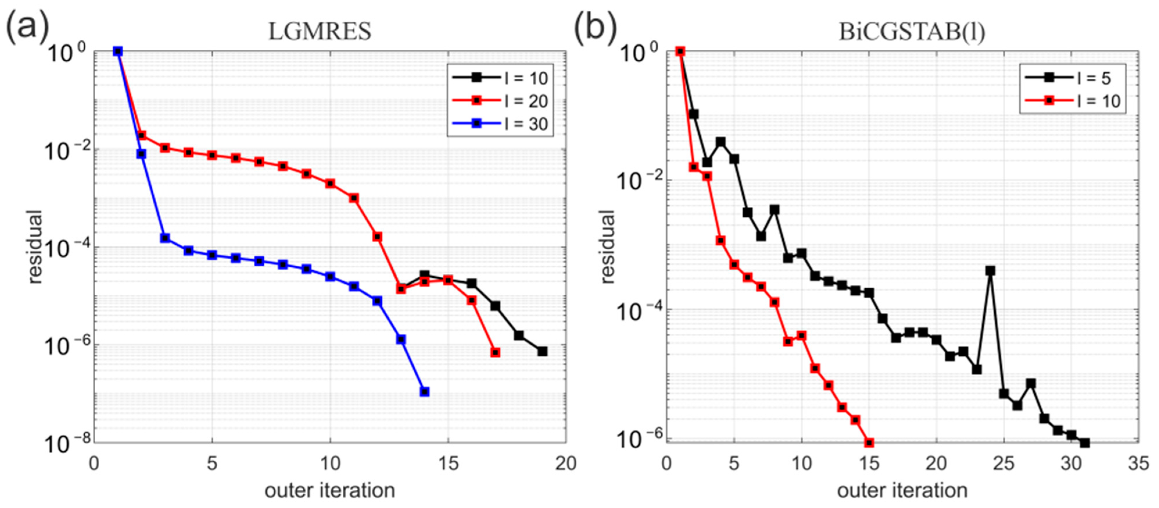
25], providing a deeper understanding of their applications in reservoirs simulations. GMRES is an extension of MINRES (which is only applicable to symmetric matrices) to non-symmetric matrices, and the iterations are based on minimizing the 2-norm of the residual vector in a corresponding Krylov subspace. Unfortunately, unlike the CG method, GMRES is based on long-term recurrence. Thus, it becomes impractical beyond a certain number of iterations in terms of memory storage. Restarted GMRES was introduced in part to circumvent this disadvantage and to keep the growth of the computational cost under control. In the restarted version of GMRES, one selects a threshold
l, and all the generated Krylov basis vectors after
l iterations are discarded. After
l iterations, a new sequence of Krylov subspaces is built using the residual,
. The resulting method is denoted as GMRES(
l). General theoretical results for the convergence rate of GMRES(
l) are not available. Restarting may slow the convergence, but when it works, it reduces storage [
10]. The iterative method LGMRES was introduced in part to potentially enhance the convergence rate of restarted GMRES. The residual vectors at the end of each restart cycle often shift direction in a repeating pattern. LGMRES applies a technique to improve the convergence of restarted GMRES by breaking this repeating pattern and acting as an accelerator for GMRES [
27].
BiCGSTAB is an extension of the BiCG method, specifically designed to address the often irregular convergence patterns observed in BiCG and CGS. The method BiCGSTAB combines elements of both BiCG and GMRES, with each BiCG step followed by a GMRES(l) iteration. Because BiCGSTAB employs short-term recurrences at each iteration, similar to CG, it generally requires less memory than GMRES. However, unlike GMRES, which minimizes the norm of the residual vector, BiCGSTAB does not guarantee any optimal property for the approximate solution vector. Consequently, as observed in our experiments, its convergence behavior can be more erratic compared to GMRES. The method BiCGSTAB(l) refers to a version where a GMRES(l) step follows each BiCG step. Although the computational cost of BiCGSTAB(l) increases with larger l, numerical experiments suggest that in some cases, the faster convergence may justify the added expense.
For nonsymmetric indefinite systems, such as those encountered in reservoir simulations, the choice of solver is delicate and problem-dependent. GMRES (without restarting) generally performs well if it converges within a few iterations, as is often the case with matrices that have a clustered spectrum [
28]. However, if GMRES requires additional iterations, it may be more effective to use LGMRES(
l) or BiCGSTAB(
l). Of course, when BiCGSTAB works, it works exceptionally well. Considering these factors, we decided to use LGMRES(
l) and BiCGSTAB(
l) as our solvers for the current study and to compare their performance for various values of
l. As previously mentioned, since the coefficient matrices arising from the discretization of the governing PDEs are typically ill-conditioned, it is important to use a preconditioner for fast convergence of a Krylov subspace method. Roughly speaking, a preconditioner is a matrix that transforms the linear system into a system that has the same solution, but the transformed coefficient matrix has a better condition number. For example, consider an (easily) invertible n-by-n matrix
P that approximates A. Then the matrix product
approximates the n-by-n identity matrix I in the sense that the eigenvalues of
are expected to be clustered around 1. Thus, the transformed system,
, is simpler than the original system, as it should be possible to do matrix-vector products of the form
at a lower cost.
There are a multitude of preconditioners that can be paired with Krylov subspace methods including Jacobi, Gauss–Seidel, algebraic multigrid (AMG), and incomplete LU (ILU) methods and their extensions/variations such as ILU(
k), ILUP(
k), ILUT(τ), and nested factorization. Moreover, there are a variety of factors that can impact the choice of a preconditioner, including suitability of the algorithms for parallel computing, physics-based implementation, and the use of structured versus unstructured grids [
29]. Many commercial solvers like Eclipse 100, IMEX, STARS, and OPM use serial or parallel versions of such ILU factorizations [
26].
Table 1.
Solver methods for MRST reservoir simulations.
Table 1.
Solver methods for MRST reservoir simulations.
| Method | Advantages | Shortcomings | CPU Time | Source |
|---|
| BiCGSTAB | Stable and efficient for large-scale simulations | May require more iterations | Longer with more iterations | [10,23,26] |
| GMRES | Robust with good convergence | Memory-intensive | Longer due to memory needs | [23,26,27,28] |
| BiCGSTAB (l) | Enhanced stability, fewer iterations | Complexity increases per iteration | May increase with complexity | [23,26,28] |
| LGMRES | Improved convergence for certain problems | Increased memory usage | Longer due to memory needs | [27,28] |
| FGMRES | Flexible with preconditioning | Requires careful tuning of preconditioners | Shorter if well-tuned | [10,27,28] |
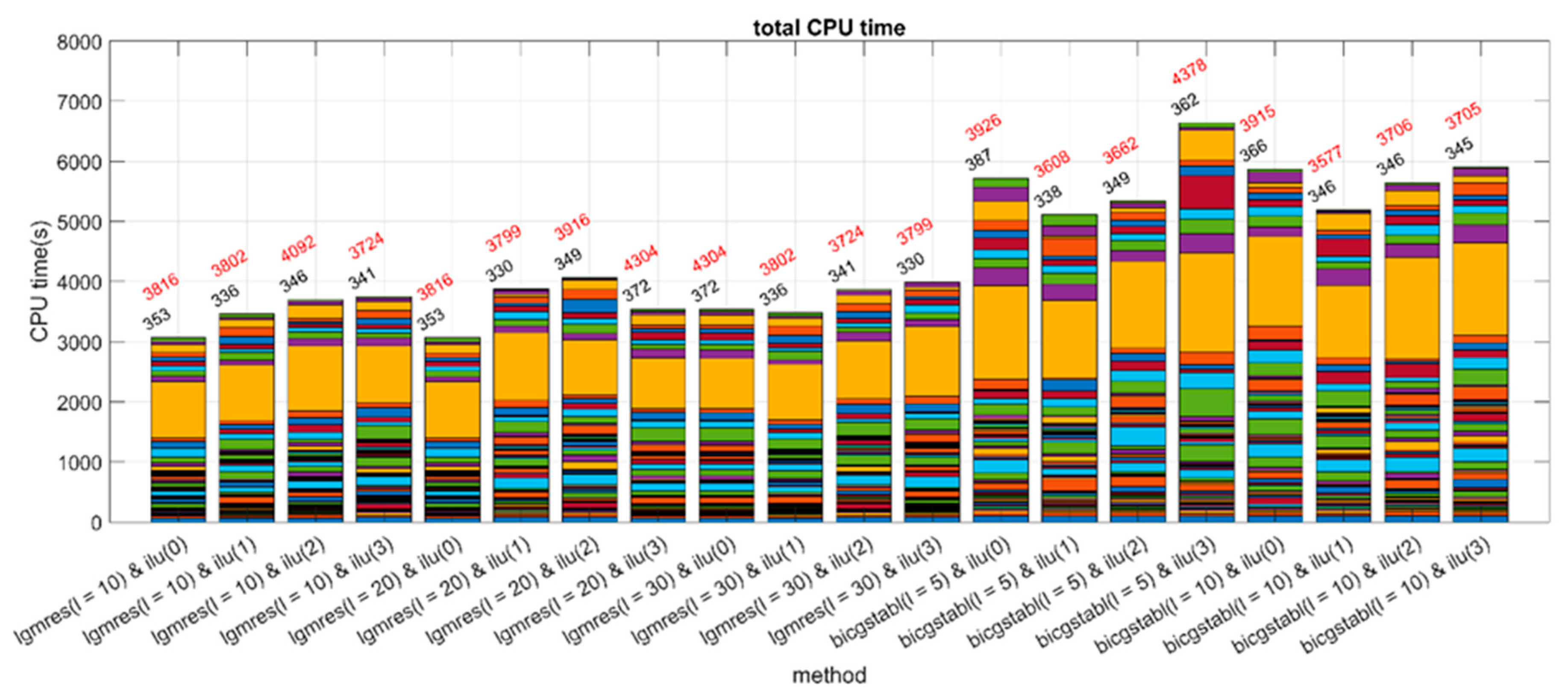
In most practical reservoir simulation scenarios, Gauss–Seidel and Jacobi preconditioners may offer some benefits, but they should not be expected to have a significant impact [
10]. On the other hand, if the problem can theoretically be stably factored into LU, the incomplete LU preconditioner is likely to improve the convergence rate. Indeed, ILU is commonly used as the default preconditioner in commercial software like COMSOL. In this study, we have employed a variant of ILU factorization, ILU(k), as our preconditioner, due to its simplicity, low setup cost, and robust performance in the presence of strong coupling and heterogeneity, which are typical features of reservoir simulations. It should be noted that although multigrid methods like AMD can be highly efficient for solving a wide range of symmetric positive definite (SPD) problems, achieving similar performance for non-SPD matrices or for large scale heterogeneous problems remains an open challenge [
29,
30].
A generic ILU algorithm can be derived from the exact LU decomposition by introducing rules that replace some aspects with zeros in the factors L and U. In ILU(0), the zero pattern for the triangular factors L and U matches exactly the zero pattern of the matrix A. However, the accuracy of ILU(0) may be insufficient to ensure a satisfactory convergence rate. More accurate incomplete LU factorizations tend to be both more efficient and reliable. For example, ILU(1) is obtained by extending the zero pattern for the triangular factors to the zero pattern of the product , where and are derived from ILU(0). Incomplete factorizations that rely on sparsity patterns are insensitive to numerical values because the elements that are dropped depend solely on the zero structure of A. In contrast, ILUT(τ), the preconditioner chosen for this study, drops elements during the Gaussian elimination process based on their magnitude rather than their position. An element is replaced by zero if it is smaller than the relative tolerance , which is calculated by multiplying τ by the original 2-norm of the row.
It is noteworthy that the system of equations originating in reservoir simulations typically exhibits a mixed elliptic/hyperbolic character, with the pressure block being nearly elliptic and the saturation/concentration part being almost hyperbolic. There are indeed matrix structuring approaches that leverage the relative homogeneity of blocks within the coefficient matrix, based on their elliptic behavior (e.g., pressure variables), hyperbolic behavior (e.g., saturations), or hybrid character (e.g., temperature). For example, constrained pressure residual (CPR) framework can be used to take advantage of the partitioning of the coefficient matrix into pressure and saturation components. One can conduct first-stage pre-conditioning for pressure variables before a full-system preconditioning and even combine CPR with other preconditioners like AMG [
26,
29,
30,
31].
In this simulation study, which is essentially a 2D field-scale project from the 11th SPE CSP, our focus has been on LGMRES and BiCGSTAB solvers along with ILU(k) preconditioners which improve their efficiency and convergence properties. Moreover, they can be easily implemented via the MRST package using the AMGCL [
31] solver library. Our simulation procedure and results are described in the next section.
2.3. Simulation Deck Description and Computations
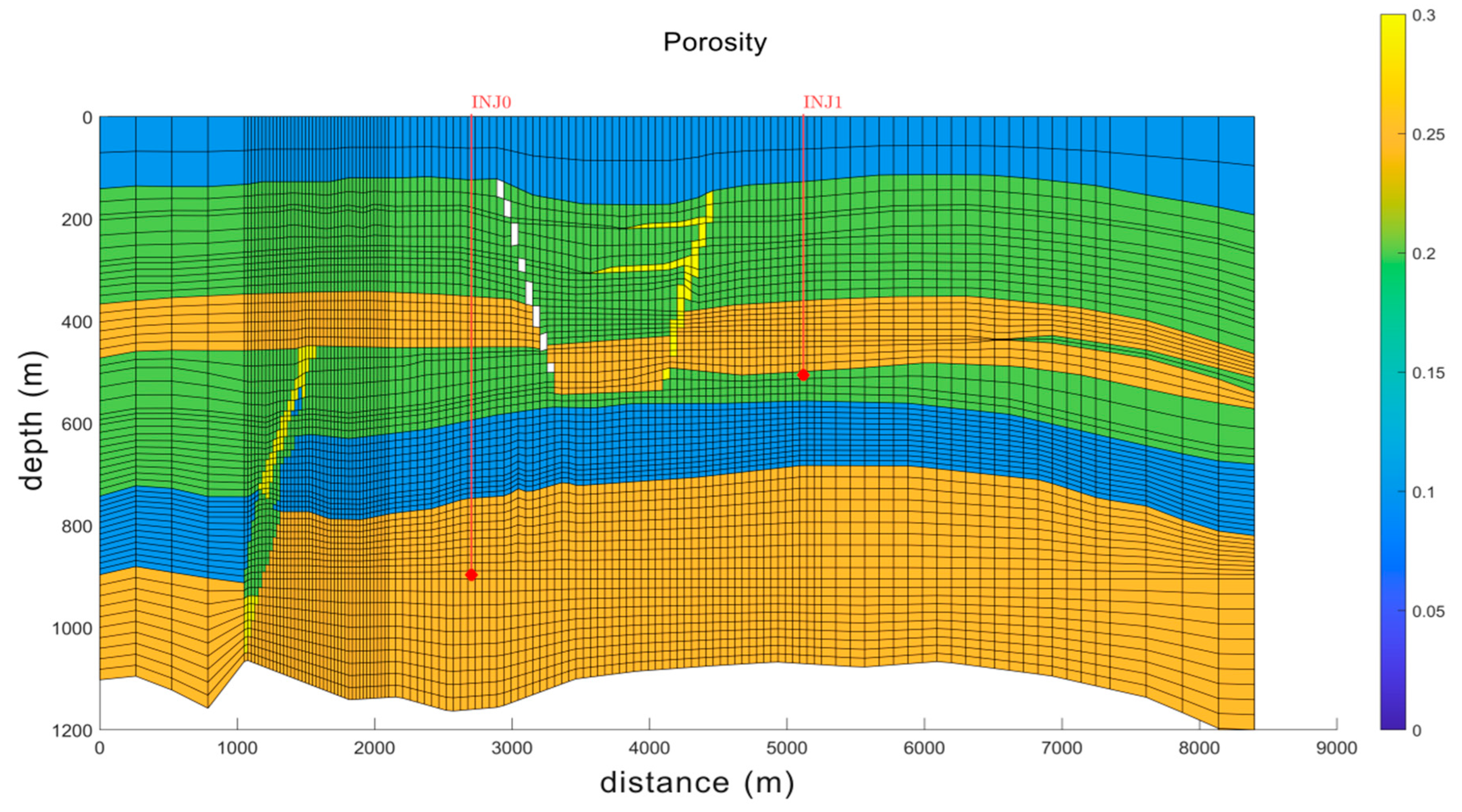
The CSP11B is designed as a two-dimensional cross-sectional representation with grid dimensions of 130 × 1 × 62, comprising 130 cells in the X direction, a single cell in the Y direction, and 62 cells in the Z direction. The overall dimensions consist of a vertical cross-section measuring 8.4 km horizontally and 1.2 km vertically. The geometry includes three fault-like structures with varying permeability: two have high permeability, while one has low permeability. This configuration allows for detailed vertical and horizontal resolution, making it particularly effective for studying vertical CO2 migration and trapping mechanisms within stratified formations.
Permeability and porosity are critical for accurately modeling the reservoir. The geometry includes seven facies, six of which are permeable and one that is impermeable. These facies define the reservoir porosity (
Figure 4) and permeability (
Figure 5), which are synthetic and represent the typical characteristics of storage reservoirs on the Norwegian Continental Shelf. Permeability in the Y and Z directions is derived from the X direction, ensuring uniformity and simplifying data input. The model defines initial equilibrium conditions with a reservoir pressure of 196.2 bars and a reference temperature of 60 °C. These parameters provide a realistic basis, closely mirroring actual reservoir conditions.
Since the properties of brine-CO2 mixtures are not well-characterized in literature, salts and minerals are excluded to simplify the problem and to avoid complications from salt precipitation and other geochemical processes. Thermal effects are also excluded to account for the fact that CO2 is often injected at temperatures lower than the reservoir’s. Detailed rock and fluid property data, such as relative permeability, capillary pressure, and fluid phase behavior, are utilized to capture the complex interactions within the reservoir.
The simulation includes a plan for gas injection through two wells, INJ0 and INJ1 (in
Figure 4 and
Figure 5), each set to inject gas at a rate of 1618.47 Sm³/day with a maximum injection pressure of 400 bars, which is selected to prevent any phase transition from water to vapor with given reservoir conditions [
18]. The simulation operates with recurring time steps: it repeats annually for the first 44 steps, then shifts to centennial intervals for the final 10 steps to facilitate long-term analysis of the reservoir’s response to gas injection. This approach allows for monitoring key performance indicators like field pressure and gas production rates.
The simulations take detailed control parameters and tuning settings into account to maintain model stability and accuracy throughout the simulation period. This ensures that the model produces reliable and precise results, supporting informed decision-making in reservoir management and optimization.


