Article

A Probability-Based Framework for Evaluating Slope Failure Under Rainfall Using Coupled Finite Element Analysis

by
Nadarajah Ravichandran
1,* and
Tharshikka Vickneswaran
2
1
Glenn Department of Civil Engineering, Clemson University, Clemson, SC 29634, USA
2
Department of Civil and Environmental Engineering, University of Louisville, Louisville, KY 40208, USA
*
Author to whom correspondence should be addressed.
Geosciences 2025, 15(4), 118; https://doi.org/10.3390/geosciences15040118
Submission received: 19 February 2025 / Revised: 13 March 2025 / Accepted: 23 March 2025 / Published: 26 March 2025

Abstract

:
Rainfall is one of the major causes of geological hazards such as landslides and slope failures because it decreases shear strength along the failure surface and increases the driving force of the sliding mass due to the movement of the wetting front in the geological media. Deterministic limit equilibrium methods are typically used to evaluate the stability of slopes in terms of Factor of Safety (FoS), considering the worst-case scenario. However, a coupled flow deformation analysis procedure combined with a probabilistic method is required to consider the temporal and spatial variations in the soil properties due to water infiltration and to evaluate the probability of slope failure. The study aims to develop a probabilistic framework for evaluating the probability of failure of an earth slope using the response surface derived from sample data generated from a coupled flow–deformation finite element (FE) program considering uncertain rainfall characteristics. Finite slopes with 1.5H:1V and 2H:1V slope ratios composed of sandy soil were analyzed considering the possible variations in soil and rainfall parameters. Based on the FE results, a response surface was developed for the FoS as a function of soil and rainfall parameters. The response surface was utilized to generate random scenarios and calculate the failure probability using Monte Carlo Simulation (MCS). The results obtained from the MCS were compared using the First-Order Reliability Method (FORM). The results indicated that the total probability of failure predicted by MCS was closer to the probability of failure by FORM. The total probability of failure predicted from MSC and FORM were 0.0633 and 0.0640 for the 1.5:1 slope and 0.0249 and 0.0229 for the 2:1 slope, respectively. This level of probability of failure was deemed unsatisfactory to poor based on the criteria by the US Army Corps of Engineers. Therefore, the proposed framework provides a valuable tool from the probabilistic perspective for assessing the performance level of slopes subjected to uncertain rainfall conditions.

1. Introduction

Recent studies have highlighted the increasing frequency of “climate whiplash” events—rapid transitions between extreme wet and dry conditions—due to global warming. This phenomenon has been linked to severe weather patterns in various regions, including intensified storms and prolonged droughts. These abrupt climatic shifts can significantly impact slope stability and failure mechanisms, as rapid soil saturation from heavy rainfall followed by drying periods can weaken soil structures, increasing the likelihood of instability and potential failure [1]. Slope failure occurs due to various factors, including excessive rainfall, toe erosion, toe excavation, and external loading such as earthquakes. Understanding these failure mechanisms is critical for assessing stability under uncertain conditions.
Rainfall is a primary factor contributing to slope failures, as it increases pore water pressure, reduces effective stress, and alters soil strength properties [2]. Numerous studies have emphasized the need for quantitative methods to assess slope stability under extreme rainfall conditions [3,4]. A comprehensive understanding of these mechanisms is essential for developing resilient geotechnical designs and effective landslide mitigation strategies. Estimating the stability of slopes due to rainfall is complex because water infiltration alters the strength and deformation properties of the slope soil in addition to the conventional pore pressure effect through the reduction in effective stress. The strength and deformation parameters of slope soil depend on the degree of saturation and/or matric suction, which varies with time and space during rainfall. The rate of movement of the wetting front depends on the hydraulic properties of the soil, the initial degree of saturation, the characteristics of the slope surface, and the intensity and duration of the rainfall. Generally, a slope’s safety (stability) is expressed by a factor of safety (FoS), which is typically determined using a limit equilibrium analysis. The conventional approach based on the limit equilibrium concept and classical soil mechanics principles followed by a parametric study may not accurately estimate the temporal variation in the stability (i.e., the onset of slope failure during a rainfall event) and the probability of failure for possible scenarios. In such situations, a coupled flow–deformation procedure combined with a probabilistic method that considers the possible variations in geometric, soil, and rainfall parameters can be used to estimate the stability of a slope systematically and accurately.
The coupled flow–deformation finite element method is well suited for conducting stability analysis of earth slopes under realistic scenarios. Among the many programs available in the literature, PLAXIS 2D, which has a coupled flow–deformation module with pressure head and flux boundaries, was successfully used by many researchers for evaluating the temporal variation in FoS [5,6]. While it assumes plane strain conditions and may not fully capture complex three-dimensional failure mechanisms, it remains more advanced than traditional limit equilibrium methods, providing a more realistic representation of soil behavior. Despite its limitations in handling highly heterogeneous or anisotropic soils, PLAXIS 2D offers a reliable and practical approach for assessing slope stability, making it a preferred choice for many geotechnical applications. Since there are several uncertainties in the computation of slope stability, the coupled flow–deformation finite element simulation alone cannot accurately predict the slope’s stability. In such situations, the more accurate deterministic finite element simulation results can then be coupled with probabilistic methods to consider the possible variations in the factors that affect the stability of a slope. The direct integration method, point estimate method, first-order second-moment method, FORM, and MCS are some of the probabilistic methods used by researchers for estimating the reliability of slope stability [7,8]. The MCS technique is widely used to calculate the probability of failure that analytical methods cannot readily solve. The advantage of using MCS is that it provides a simple framework for the reliability analysis of the system and can be used in repetitive executions to determine the FoS systematically [9]. The MCS technique is robust to the finite element modeling (FEM) for system reliability analysis of geotechnical systems, including stability of slopes [9,10,11,12].
Several studies have been conducted to estimate the failure probability of earth slopes subjected to rainfall through mechanics-based models [2,11,12,13]. Among the many, Lu et al. [11] proposed a mechanics-based approach to estimate the annual probability of slope failure subjected to rainfall in Singapore. Their study considered the uncertainty of soil properties and annual rainfall events. The yearly rainfall events were modeled through a bivariate distribution of intensity and duration, and the MCS was used to calculate the annual failure probability. They found that for the selected slope, the slip surface was deep when the rainfall duration was small, and the critical slip surface gradually moved to the upper wetted zone when the rainfall duration increased. Liu and Wang [2] developed a probabilistic hazard analysis framework for rainfall-induced landslides, incorporating both rainfall uncertainty and soil spatial variability. They employed a fully Monte Carlo Simulation-based method to assess the annual slope failure probability at specific sites. Jiang et al. [14] developed an efficient reliability analysis method based on MCS and limit equilibrium methods (LEM) to estimate the probability of slope failures in spatially variable soils. They concluded that the proposed method estimated the probability of failure considering the spatial variability of the cohesive soil properties while improving the computational efficiency at small probability levels.
The above studies indicate that the temporal variation in stability of slopes subjected to rainfall must be analyzed in a coupled manner incorporating the possible variations in system and loading characteristics. This study develops a probabilistic framework to systematically evaluate how slope geometry, soil strength properties, and varying rainfall intensities and durations influence slope stability. Unlike broad-scale landslide hazard assessments, this research focuses on the mechanical response of slopes by analyzing shear strain, stress variations, and probabilistic failure risks under different rainfall conditions.
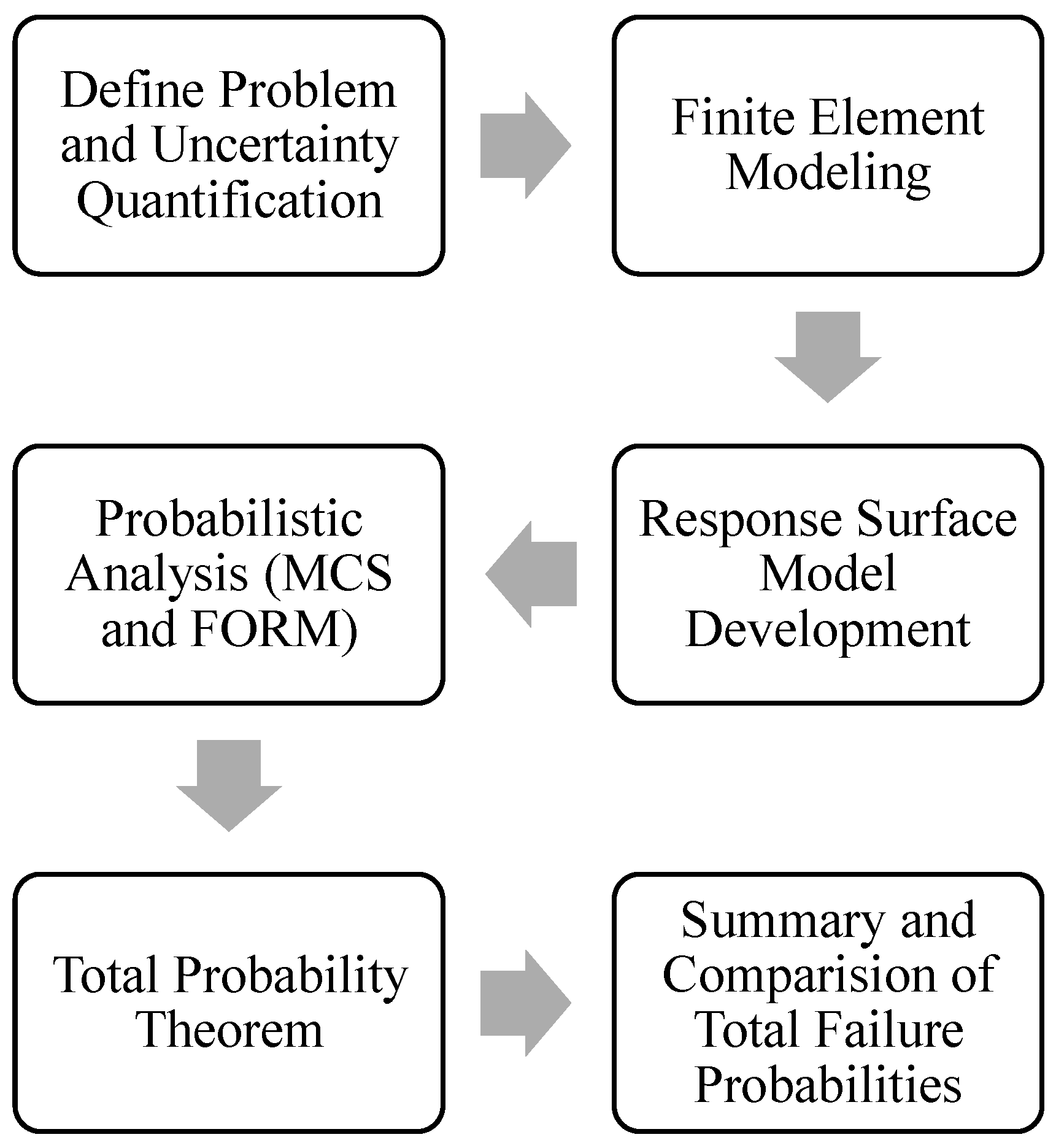
To achieve this, the variables that affect the stability of the slope were identified, and their ranges were established. Then, PLAXIS 2D, a coupled flow–deformation finite element code, was used to simulate selected scenarios by systematically varying the random variables. The finite element results were then used to develop a mathematical relationship between the Factor of Safety (FoS) and the variables, called a response surface. Finally, the Monte Carlo Simulation (MCS) technique was used to calculate the probability of failure with the response surface, and the values obtained were validated using the First-Order Reliability Method (FORM) for future applications.
The novelty of this work lies in integrating deterministic finite element simulations with a response surface model to assess slope stability under uncertain rainfall conditions systematically. This approach provides a more comprehensive understanding of the influence of rainfall intensity and duration on slope failure, bridging the gap between numerical modeling and probabilistic assessment. This framework ensures robustness and reliability by validating results using both MCS and FORM, making it a valuable tool for geotechnical risk evaluation.

2. Problem Definition

The overall research framework is summarized in Figure 1 to provide a comprehensive understanding of the study. The process begins with identifying key variables, including slope geometry, soil properties, and rainfall parameters, which serve as inputs for the analysis. The following are the key steps:
  • Identification of Input Parameters: The study considers variations in slope ratio, soil friction angle, rainfall intensity, and rainfall duration as primary factors influencing slope stability;
  • Finite Element Simulations (PLAXIS 2D): A coupled flow–deformation finite element model is used to simulate slope responses under different rainfall conditions and compute the Factor of Safety (FoS) over time;
  • Development of Response Surface Model: The finite element simulation results are used to construct a polynomial response surface equation that approximates the relationship between FoS and input parameters to facilitate probabilistic analyses;
  • Probabilistic Failure Analysis (Monte Carlo Simulation—MCS): The response surface model is integrated into MCS to estimate the probability of failure across a range of scenarios, accounting for variations in input parameters;
  • Validation Using First-Order Reliability Method (FORM): FORM is employed to compare results with MCS and evaluate differences due to assumptions in the linearization of the limit-state function;
  • Computation of Total Probability of Failure: The final failure probability is computed by integrating conditional failure probabilities with rainfall distributions, providing an overall risk assessment of slope performance under uncertain rainfall conditions.

2.1. Slope Geometry, Soil Properties, and Their Variations

This study considered two finite slopes with 1.5H:1V (SR1) and 2H:1V (SR2) slope ratios and 12 m height. The geometry and sample finite element mesh that will be discussed later for SR1 is shown in Figure 2. The slopes were assumed to be made of sandy soil with a mean friction angle of 30° and zero cohesion. Based on the literature [15], a 10% COV was assumed for the friction angle of the soil. This resulted in a standard deviation of 3° and the friction angle varies between 27° and 33° for ±1 standard deviation. Although ±3 standard deviation is typically used to cover the possible variation, ±1 standard deviation was used to avoid unrealistic geometric and soil combinations that may cause numerical instability during coupled flow–deformation finite element simulations. For example, the slope with a lower friction angle may not be stable enough to perform any finite element calculation. Although some cases would produce results, they may not produce symmetric data.
From preliminary studies, it was observed that the other soil properties, such as modulus of elasticity, Poison’s ratio, and dilatation angle, had a small effect on the computed FoS. A similar conclusion was made by Hammah et al. [16] based on their slope stability study in which elastic modulus, Poisson’s ratio, and dilatation angle were varied between 2000 and 200,000 kPa, 0.2 and 0.48, and 0 and 35°, respectively. Another study by Mahmoudabadi and Ravichandran [17] also concluded that the variation in Poisson’s ratio can be ignored for sandy soils. Cheng et al. [18] concluded that the dilation angle and modulus of elasticity had insignificant effects on slope stability. Based on the literature, a dilation angle of zero, Poison’s ratio of 0.3, and modulus of elasticity of 30 MPa were assumed for the sandy soil in this study, and their variations were not considered [19].

2.2. Rainfall Intensity, Duration, and Their Variations

The daily rainfall data from 1979 to 2020 at 3812 stations in the US, as shown in Figure 3, was obtained from the Global Historical Climatology Network Daily (GHCNd). The selected period from 1979 to 2020 ensures a sufficiently long historical record to capture rainfall variability, extreme events, and long-term climatic trends. This timeframe provides a statistically robust dataset for probabilistic analysis, allowing for the evaluation of rainfall intensity variations that influence slope stability.
Based on the data, the mean and standard deviation of the rainfall intensities were 410 mm/day and 80 mm/day, respectively. The ±1 standard deviation resulted in three rainfall intensities of 330 mm/day, 410 mm/day, and 490 mm/day for lower, mean, and upper estimates, respectively. The rainfall data were assumed to be normally distributed, and the normal distribution fitted to the measured rainfall data is shown in Figure 4.
The duration of these rainfalls varied between 1 and 10 days. The trial simulations confirmed that the 10 days of infiltration was long enough for the wetting front to reach the potential critical failure surface. It was assumed that there was no surface runoff and all the rainfall infiltrated the soil.

3. Coupled Flow–Deformation Finite Element Model

3.1. Modeling Tool

Since the slope stability problem involves interaction between the flow of water through the soil and the shear strength and deformation parameters of the soil, a coupled flow–deformation finite element formulation is required to accurately evaluate the temporal variation in FoS during rainfall and water infiltration. This study used the coupled flow–deformation module available in PLAXIS 2D to compute the temporal variation in FoS for a given scenario. The coupled governing equations, finite element formulation, and coupling procedures can be found in the PLAXIS 2D manual [20]. The strength reduction method (SRM) is implemented to compute the FoS of the slope at a selected time. The strength reduction method (SRM) implemented in PLAXIS is used to determine the Factor of Safety (FoS) for slopes under rainfall conditions. In this approach, the shear strength parameters of the soil—cohesion (c) and internal friction angle ( ϕ )—are systematically reduced by dividing them by a strength reduction factor (SRF). The SRF is progressively increased until the numerical model indicates failure, typically defined by excessive deformations or non-convergence in the simulation. The SRF value at failure represents the FoS for the given slope. This method is widely used for slope stability analysis due to its robustness and ability to simulate realistic failure mechanisms. The SRM implementation in this study uses an elastoplastic Hardening Soil (HS) model for the soil behavior, ensuring an accurate representation of stress–strain relationships.

3.2. Stress–Strain Model

An accurate mathematical representation of the true behavior of the soil under varying moisture content is required to evaluate the slope behavior using the finite element method. Also, for the slope stability problem, the strain varies significantly within the simulation domain. A strain near failure is expected along the failure surface, but it can be almost zero away from the failure surface. Since the soil behaves nonlinearly, even at small strains, a nonlinear stress–strain model must be used to evaluate the deformation and stability of the slope accurately. In this study, the nonlinear elastoplastic Hardening Soil (HS) model, shown in Figure 5, was used to represent the stress–strain behavior of the soil. The HS model considers the modulus reduction with strain compared to the widely used simple Mohr–Coulomb model, which is a linear elastic, perfectly plastic model.
The key HS model parameters are the (i) secant modulus at 50% of the failure stress ( E 50 r e f ), (ii) tangent modulus for primary oedometer loading ( E o e d r e f ), (iii) unloading/reloading modulus ( E u r r e f ), (iv) power of stress level dependency of modulus ( m ), (v) effective cohesion ( c ), (vi) effective friction angle ( ϕ ), and (vii) Poisson’s ratio ( ν ). All the moduli correspond to the reference (ref) confining pressure of 100 kPa ( p r e f ). The HS model parameters and the other soil properties used in this study are tabulated in Table 1.

3.3. Suction–Moisture Model and Hydraulic Conductivity of Unsaturated Soil

The temporal variation in FoS of the stability of slopes subjected to rainfall involves unsaturated soils. A suction–moisture model must be used to relate the suction at different moisture content or degrees of saturation. Among the many models available in PLAXIS, the van Genuchten [21] model, shown in Equation (1), was used in this study.
S ( ψ ) S r e s ( S s a t S r e s ) = 1 + ( g a | ψ | g n g c
where ψ is the matric suction, S ( ψ ) is the degree of saturation of the soil at suction ψ , S r e s is the residual degree of saturation, S s a t is the degree of saturation at a fully saturated state, g a , g n , and g c are model parameters. g a is a model parameter related to the air entry value of the soil, g n is related to the rate of water extraction from the soil once the air entry value has been exceeded, and g c is related to g n as follows: g c = ( 1 g n ) / g n .
The unsaturated hydraulic conductivity ( k u n s a t ) is the multiplication of the hydraulic conductivity at the fully saturated state ( k s a t ) by the relative hydraulic conductivity at the unsaturated state ( k r ), as shown in Equation (2). Mualem-van Genuchten [21] proposed the model, shown in Equation (3), for the relative hydraulic conductivity based on the corresponding SWCC.
k u n s a t = k r k s a t
k r ( S ) = ( S e ) g l 1 1 S e g n g n 1 g n 1 g n 2
where S e is the effective degree of saturation i . e . ,   S e = S S r e s S s a t S r e s . The hydraulic properties of the soil considered in this study are tabulated in Table 2. The soil water characteristic curve (SWCC) and the unsaturated hydraulic conductivity are shown in Figure 6.

3.4. Finite Element Model Development

A two-dimensional plane strain model was used to represent the slope numerically in PLAXIS 2D. The deformation and flow boundaries, including no flow (closed) through the vertical sides and the base, were applied numerically to the simulation domain to replicate field conditions. That is, the bottom and the top of the slope are horizontal, and the flow is one-dimensional (vertically down) near the boundaries. In contrast, two-dimensional flow occurs near the slope face. The displacement boundaries include fixing the vertical sides in the horizontal direction (free to move in the vertical direction) and the base in both vertical and horizontal directions. The simulation domain was discretized spatially using 15-node triangular plane strain elements. The mesh near the slope face, horizontal surfaces, and potential failure surfaces were refined to accurately capture the high infiltration and deformation gradients. As the finite element results are sensitive to the simulation domain and element (mesh) sizes, domain size, and mesh size sensitivity studies were conducted to determine a suitable simulation domain size and corresponding mesh size such that these user-controlled parameters do not alter the computed responses. The final simulation domain size and the finite element mesh are shown in Figure 2.

4. Deterministic Analysis Using Finite Element Method and Calculation of Temporal Variation in Fos

The gravity loading function was used to generate the initial stresses and pore pressures by applying the self-weight of the slope. One hundred and seventy finite element analyses of several scenarios were carried out that include two slope ratios (SR1 and SR2), three friction angles (27°, 30°, and 33°), three rainfall intensities (0.33 mm/day, 0.41 mm/day, and 0.48 mm/day), and ten rainfall durations (1 to 10 days with an interval of 1 day). The study by Vickneswaran and Ravichandran [22] shows evidence of the ten-day rainfall-inducing landslide in a case study of the Meeriyabedda, Sri Lanka landslide.

4.1. Effect of Rainfall Intensity and Duration on the Stability of Slopes

4.1.1. 1.5:1 Slope (SR1)- Influence of Rainfall Intensity and Duration

Figure 7a–c show the variation in FoS with time for friction angles 27°, 30°, and 33°. The figure shows that the FoS decreases with time for all three rainfall intensities but with different gradients. The slope with a friction angle of 27° failed at the end of four, five, and six days for the rainfall intensities of 490 mm/day, 410 mm/day, and 330 mm/day, respectively, as seen in Figure 7a. The slope with a friction angle of 30° failed at the end of six and ten days for intensities of 490 mm/day and 410 mm/day, respectively, and the slope did not fail for the lowest intensity of 330 mm/day, as seen in Figure 7b. From the figure, it was observed that the slope with a 33° friction angle did not fail during the rainfall event.

4.1.2. 2:1 Slope (SR2)- Influence of Rainfall Intensity and Duration

Figure 8a–c show the variation in FoS with time for friction angles 27°, 30°, and 33°, respectively. The figure shows that the FoS decreases with time for all three rainfall intensities but with different gradients. The results show that none of the slopes failed during ten days of rainfall. The initial FoS of 1.45 for the slope with a friction angle of 27° reduced to 1.31, 1.29, and 1.24 at the end of ten days of rainfall for intensities of 330, 410, and 490 mm/day, respectively. The initial FoS of 1.58 for the slope with a friction angle of 30° reduced to 1.42, 1.32, and 1.30 at the end of ten days of rainfall for intensities of 330, 410, and 490 mm/day, respectively. The initial FoS of 1.76 for the slope with a friction angle of 33° reduced to 1.57, 1.51, and 1.48 at the end of ten days of rainfall for intensities of 330, 410, and 490 mm/day, respectively.

4.2. Effect of Friction Angle on the Stability of Slopes

4.2.1. 1.5:1 Slope (SR1)

Figure 9a–c show the temporal variation in FoS for rainfall intensities of 330, 410, and 490 mm/day, respectively, for friction angles 27, 30, and 33°. The results show that the slope with a friction angle of 27° failed at the end of 6 days, and others did not fail, although the FoS gradually decreased.

4.2.2. 2:1 Slope (SR2)

Figure 10a–c show the temporal variation in FoS for rainfall intensities 330, 410, and 490 mm/day, respectively, for friction angles 27, 30, and 33°. The results show that none of the slopes failed during the rainfall event.

5. Probabilistic Analysis and Calculation of Probability of Failure

The probabilistic approach can systematically incorporate the uncertainties in soil properties and rainfall intensity and duration in the computation of slope stability for real-world applications. Among the many methods available in the literature for developing relationships between more than one variable, the response surface method (RSM) has been proven to be a computationally efficient method for slope stability analysis and other engineering problems [23]. Kumar et al. [24] applied Response Surface Methodology (RSM) to assess the stability of three real-world rock slopes with varying failure mechanisms, demonstrating its effectiveness in reliability-based slope analysis. By comparing RSM-based reliability estimates with Monte Carlo Simulation (MCS), the study confirmed the accuracy and computational efficiency of different response surface techniques, providing guidelines for selecting the most suitable RSM approach for practical geotechnical applications. Li et al. [23] evaluated the computational accuracy and efficiency of various response surface methods (RSMs) for different types of slope reliability problems, confirming their applicability in real-world geotechnical assessments. The study demonstrates that RSMs provide reliable and computationally efficient alternatives for slope stability analysis under uncertainty by comparing single and multiple response surface approaches across multiple-layered and spatially variable soil conditions. RMSs involve fitting a polynomial model to the observed data (computed data in this case) and using it to find the response (FoS in this case) over a wide range of independent variables.

5.1. Development of Response Surface

The FoS were calculated based on 170 coupled flow–deformation finite element simulations considering several scenarios by varying the slope ratios, friction angles, rainfall intensities, and rainfall durations (random variables). The FoS was then expressed as a function of random variables using multiple linear regression of approximation, as shown in Equation (4). Among the many models commonly used for developing a response surface, the second-order polynomial model was used in the study. Equation (4) has fourteen coefficients (1 constant, 4 linear term coefficients, 6 two-factor interaction coefficients, and 3 quadratic term coefficients).
F o S = 2.971 + 0.39 R I + 0.0194 R D 0.1024 F A + 0.0038 S A 0.36 R I × R I 0.000087 R D × R D + 0.003018 F A × F A 0.1003 R I × R D + 0.017 R I × F A 0.0232 R I × S A 0.000292 R D × F A + 0.000433 R D × S A 0.001509 F A × S A
where SA is the slope angle (in degrees), RI is the rainfall intensity (in m/day), RD is the rainfall duration (in days), and FA is the friction angle (in degrees). As expressed in Equation (4), the second-order polynomial model was selected to capture the nonlinear relationships among the random variables influencing the Factor of Safety (FoS), including slope angle, rainfall intensity, rainfall duration, and soil friction angle. The coefficients of the model were estimated using multiple linear regression based on 170 coupled flow–deformation finite element simulations covering a wide range of parameter variations.
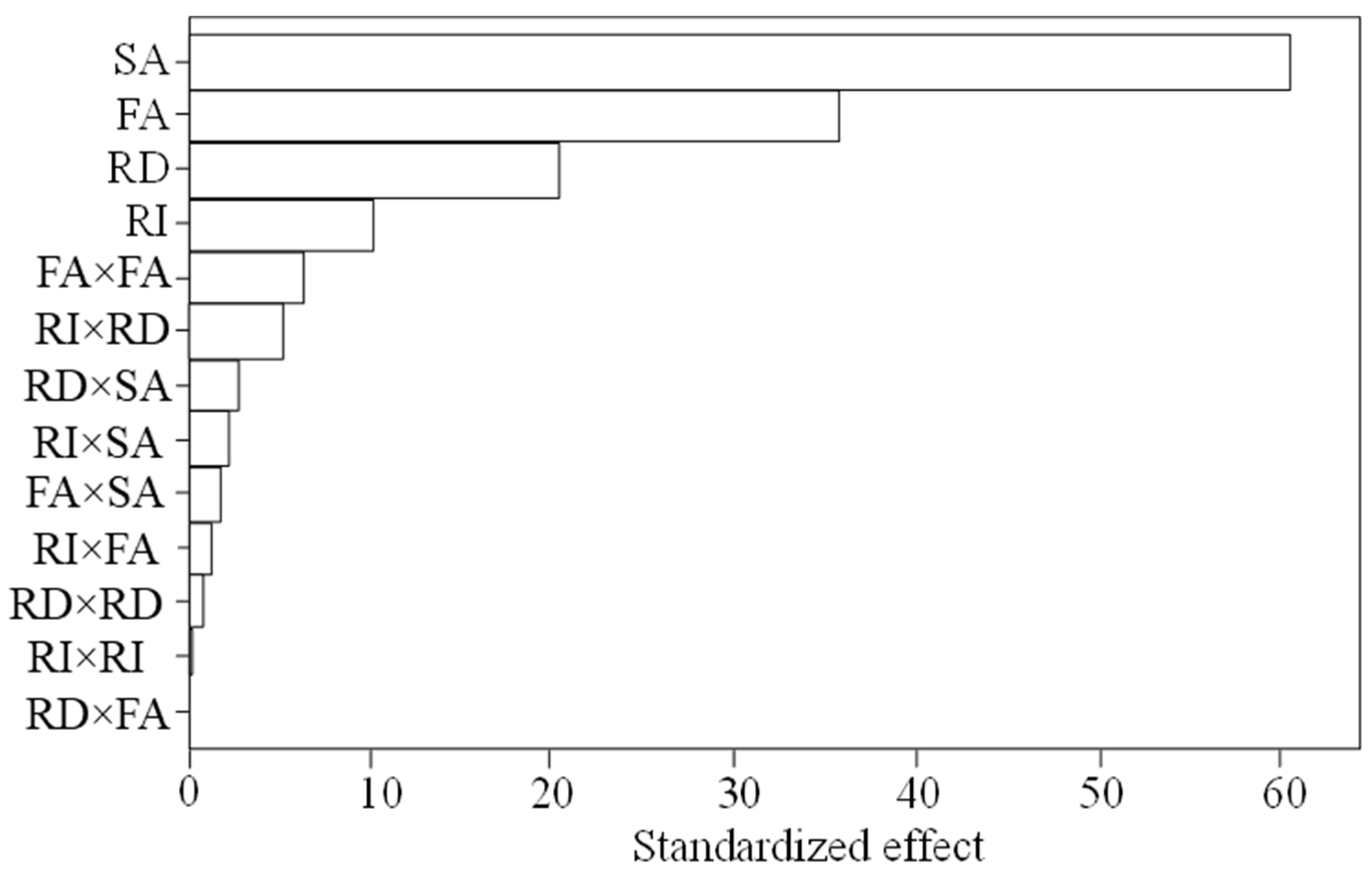
To assess the significance of each variable, a standardized Pareto chart was generated (Figure 11). This chart highlights the dominant effects of slope angle (61%) and friction angle (36%) on the response, while rainfall intensity and duration showed relatively lower influence. The Pareto chart was derived to show the impact of each variable considered in this study. Regarding the effect of individual random variables, it is clear that SA has the strongest influence on FoS (61). The next influential variable is the FA, which shows almost ¾th impact (36) compared to SA. The RI has the least influence on slope stability compared to the other random variables. The quadratic relation of FA and RD showed the least impact on the FoS.
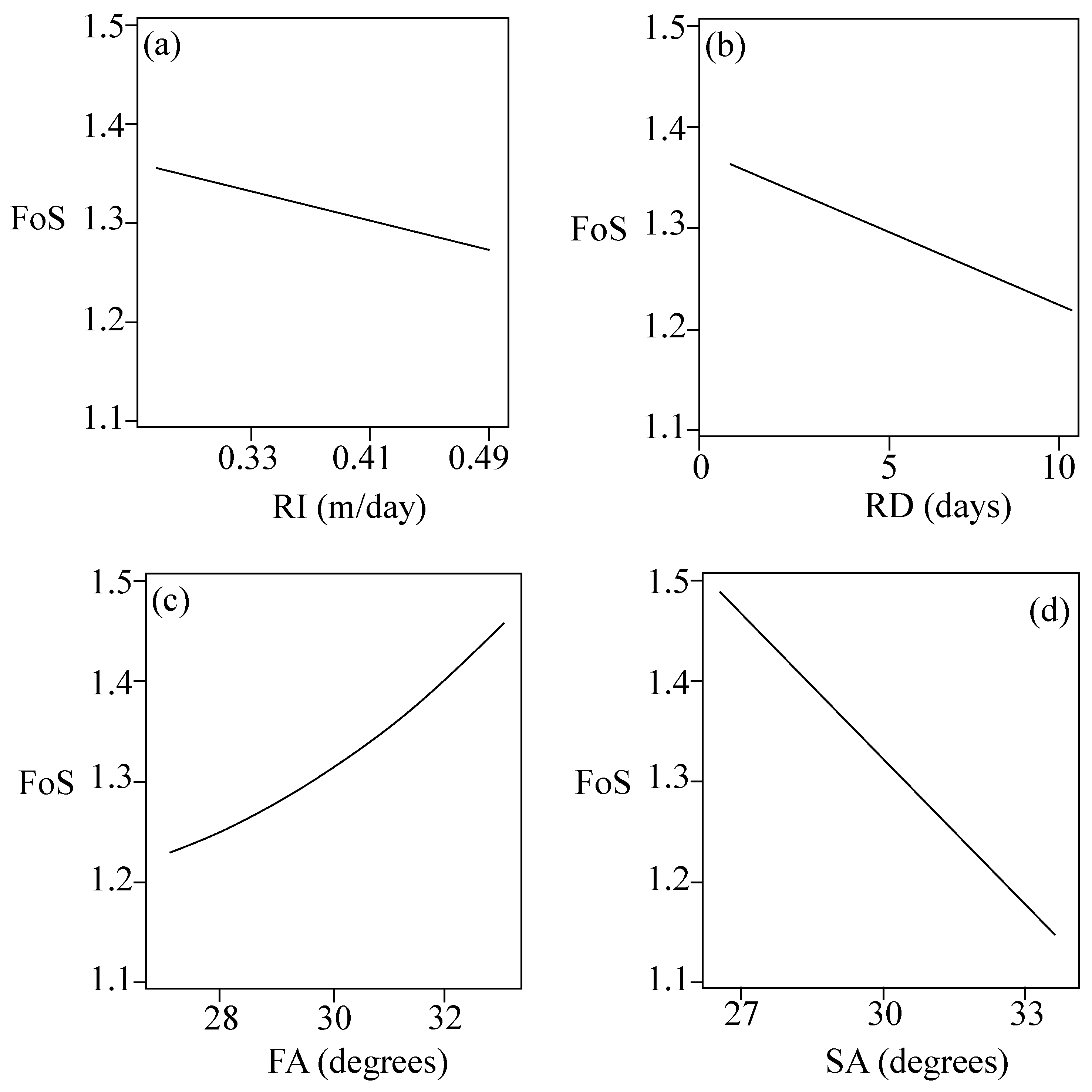
The influence of each random variable on FoS is shown in Figure 12. From the figure, the impacts of RI, RD, and SA on FoS are linear, while FA is nonlinear. It is also observed that the FoS decreases with RI, RD, and SA while it increases with FA.
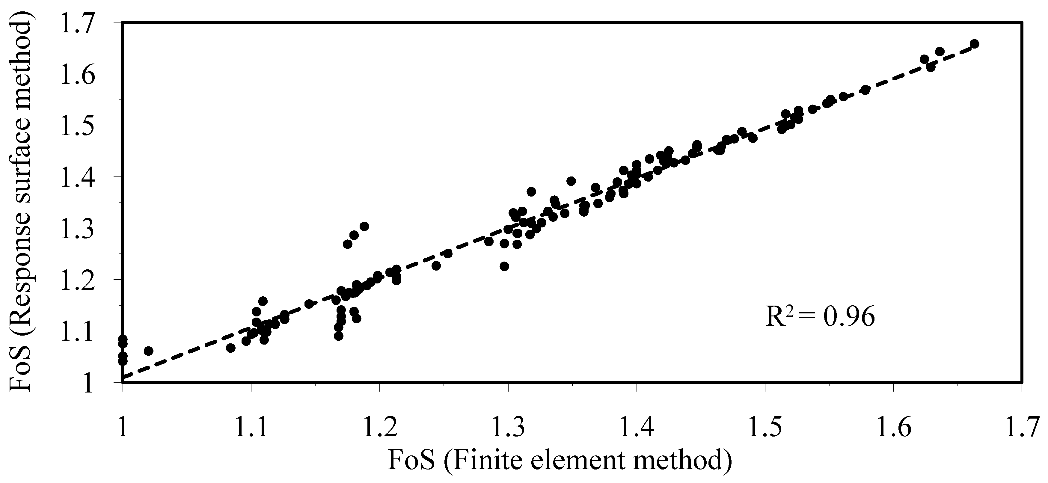
The second-order polynomial model effectively approximates the behavior of the system, as demonstrated by the high R2 value (0.96) when comparing the modeled and simulated FoS values (Figure 13). This ensures the reliability of the model for subsequent probabilistic analyses. Figure 13 compares the FoS calculated from the response surface equation (Equation (4)) and computed from the finite element method. A high R2 value (0.96) shows that the mathematical model fits the data generated from the finite element method reasonably well and can be used for further study.

5.2. Bivariate Distribution of the Probability of Rainfall Intensity and Duration

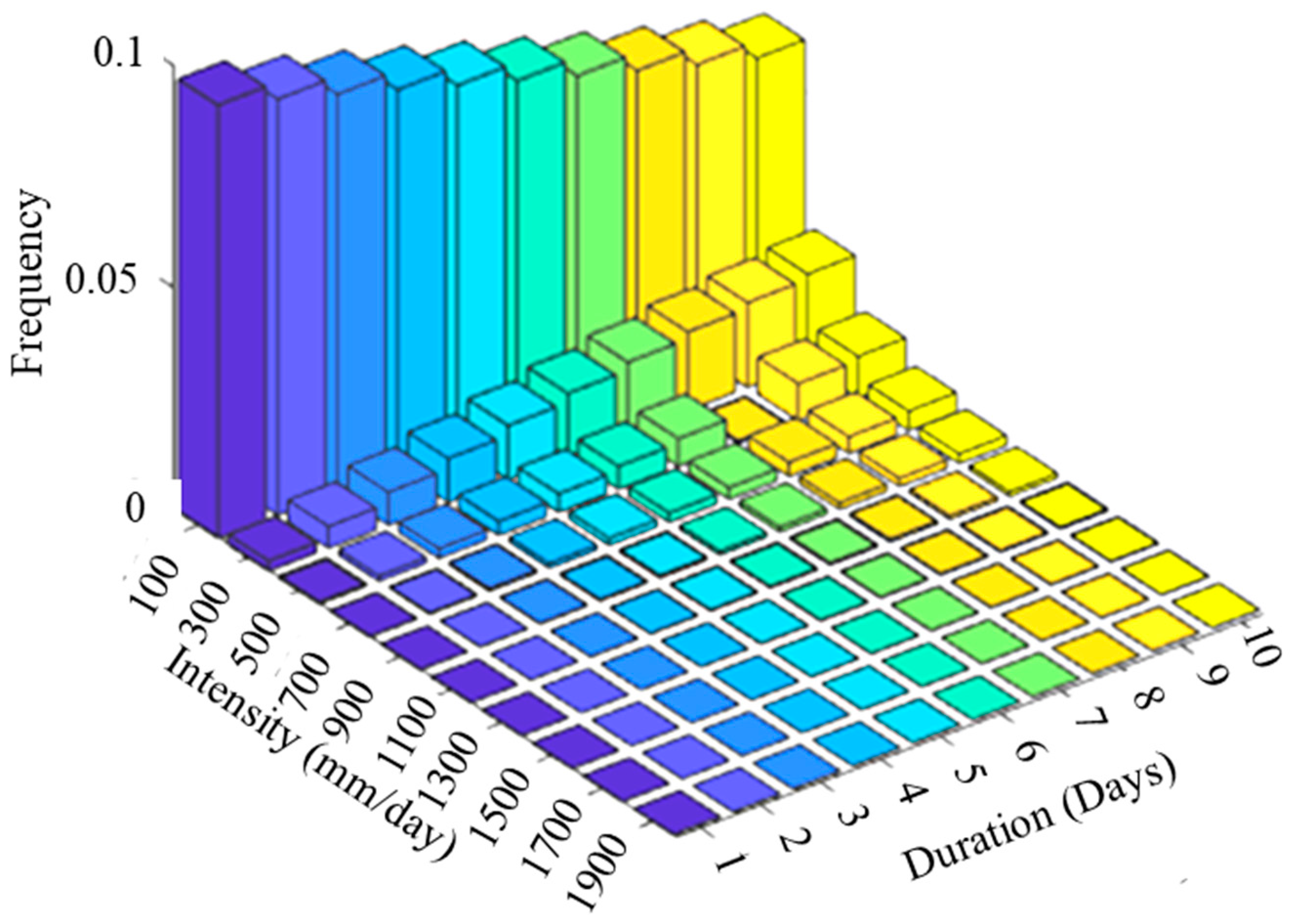
The daily rainfall data from 1979 to 2020 for 3812 stations in the US was obtained from Global Historical Climatology Network Daily (GHCNd). The relative frequency of intensity and duration were obtained from this rainfall data, as shown in Figure 14. The results show that the frequency of the lowest rainfall intensity (200 mm/day) with the shortest duration (1 day) was higher than the other rainfall intensity and duration combinations. The lowest frequency was obtained for the higher intensity (2000 mm/day) and most prolonged duration (10 days). Therefore, this study adopts the bivariate distribution of intensity and duration to calibrate the uncertainty performance with daily rainfall events.

5.3. Calculation of Probability of Failure Using Monte-Carlo Simulation

The response surface developed in the previous section was used to calculate the probability distribution of FoS for a wide range of random variables. The Monte Carlo Simulation (MCS) approach was implemented to estimate the probability of failure, defined as the conditional probability of failure for given combinations of rainfall intensity and duration. The MCS procedure consisted of two main steps. First, 10,000 random samples of each random variable (rainfall intensity, rainfall duration, and soil friction angle) were generated. These samples were drawn from a log-normal distribution, which is commonly used in geotechnical engineering due to its ability to represent non-negative variables and capture the natural variability of soil properties. The log-normal distribution was selected because soil parameters, particularly friction angle, and permeability, often exhibit a positively skewed distribution in field measurements. After generating the random samples, each sample was substituted into the response surface function (Equation (4)) to compute the corresponding FoS values. This probabilistic approach enabled the estimation of failure probabilities under various rainfall conditions. The probability of failure in this study was then calculated using the equation shown in Equation (5). The impact of input distribution variations was further assessed through sensitivity analysis, ensuring that the probabilistic results remained representative of real-world geotechnical conditions.
P f = 1 N i = 1 N I ( F o S ( x i ) < 1 ) = N f N
where P f is the probability of failure, I is the indicator function (Equation (4)), x i is the uncertainty parameter (random variable), N is the number of random samples, and N f 
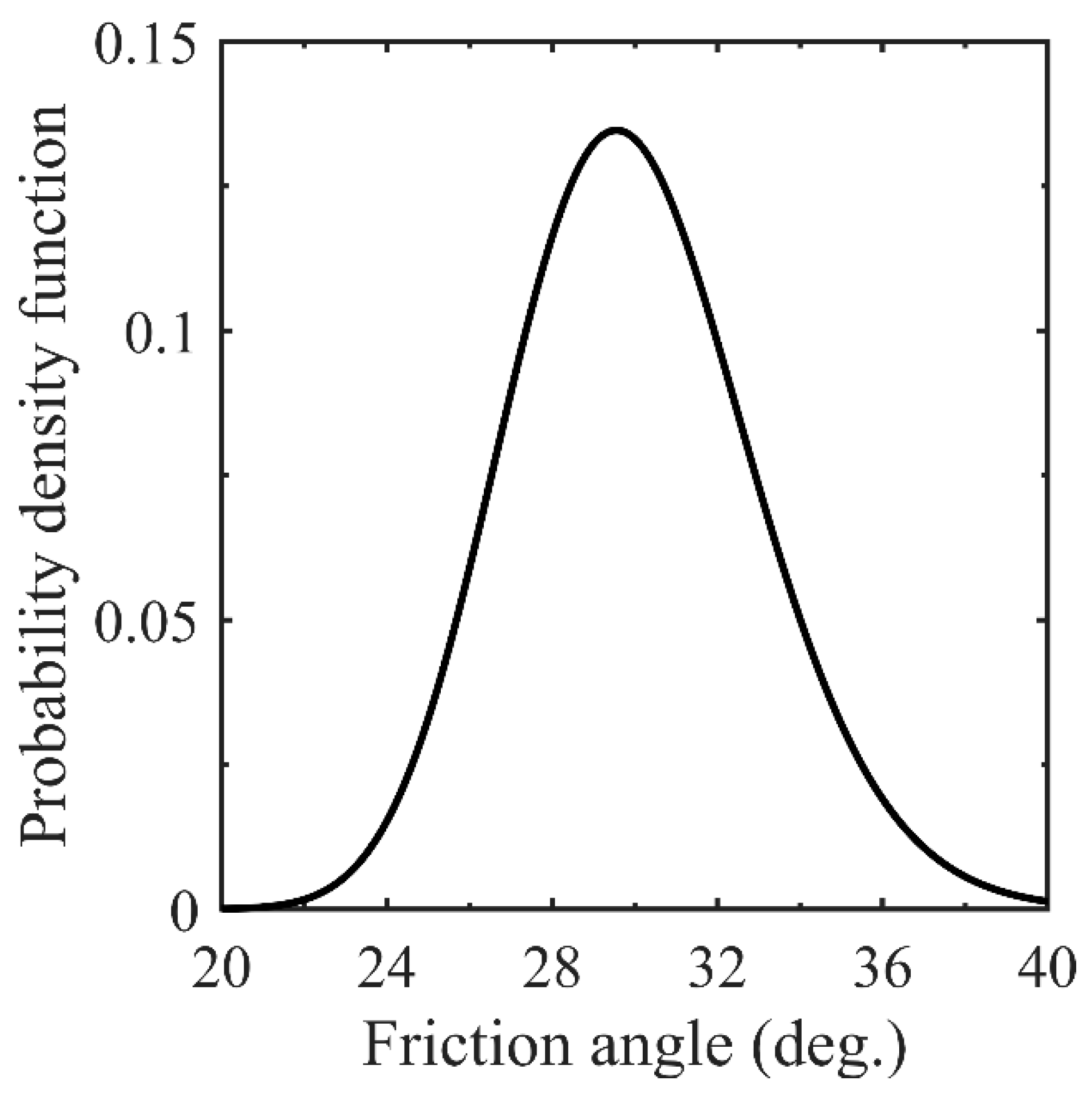
is the number of failure samples. In the Monte Carlo Simulation (MCS) procedure, 10,000 random samples of input parameters were generated using the Latin Hypercube Sampling (LHS) technique to ensure statistical robustness and efficient representation of variability. The soil friction angle was assumed to follow a log-normal distribution with a mean of 300 and a standard deviation of 30, as variations in grain size, density, and compaction naturally lead to this distribution for sandy soils. This choice aligns with published studies that indicate friction angles for sandy soils typically exhibit log-normal behavior. To ensure a realistic representation of field conditions, random values were generated within a broader range of 200 to 400, extending beyond the values used in finite element simulations, thereby accounting for potential variability observed in geotechnical practice. Rainfall intensity and duration were modeled using a bivariate distribution to capture their statistical dependence based on historical rainfall data, as shown in Figure 15. Sensitivity analysis confirmed that slope angle and soil strength parameters had the highest influence on stability, while rainfall variations contributed to increased uncertainty in failure probabilities. By incorporating well-calibrated distributions and a wide range of values, the probabilistic framework enhances the reliability of failure probability estimates, making the approach more applicable to practical geotechnical risk assessments.

5.4. Procedure for Determining the Total Probability of Failure

The probability of failure for rainfall-induced slope instability was estimated by calculating the number of failures using Equation (4), where FoS falls below 1 for different rainfall intensity, duration, and friction angles. The probability of failure was obtained separately for both slope ratios. Figure 16 shows the procedure adopted for calculating the probability of failure.
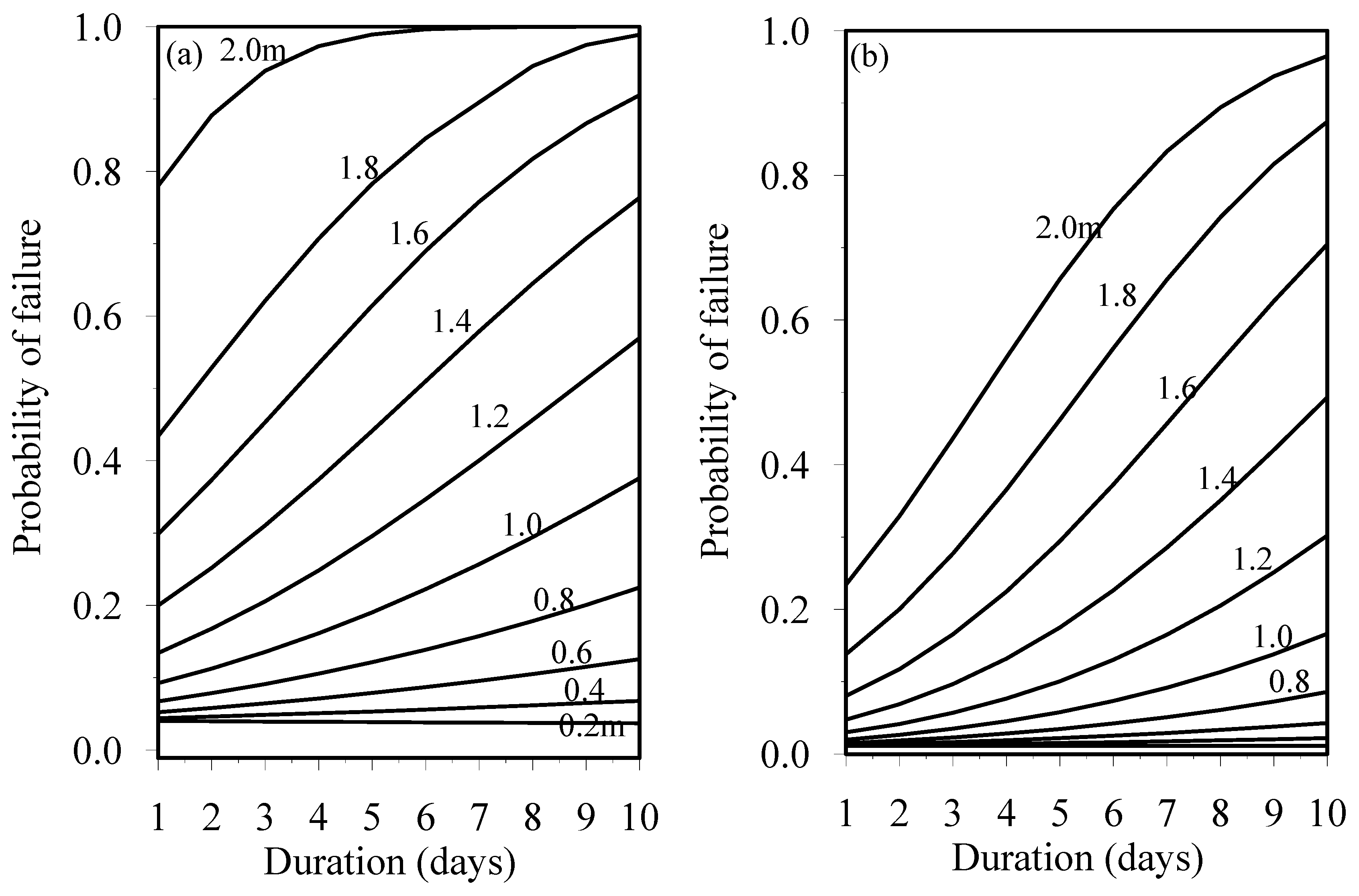
Figure 17a,b show the calculated probability of failure for each intensity and duration for SR1 and SR2 at randomly selected friction angle values using MCS. 
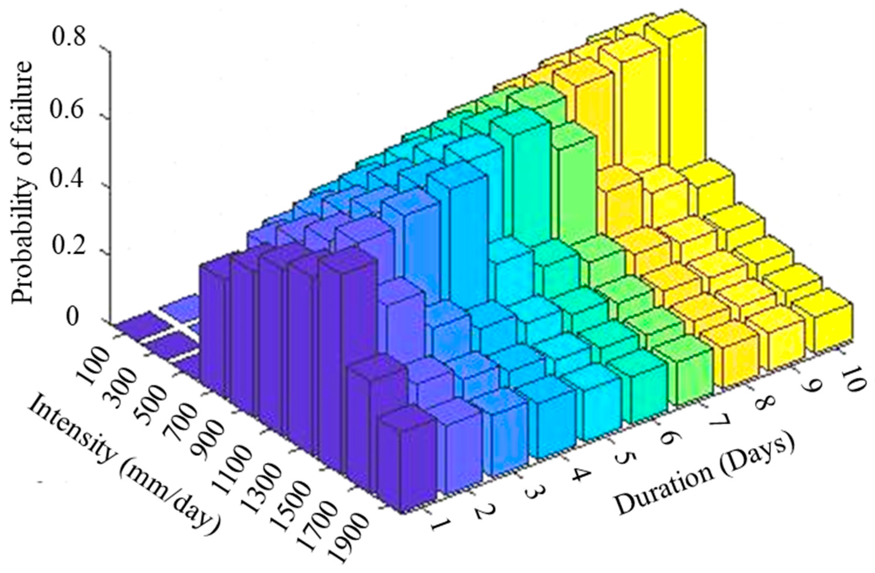
Figure 18 shows that the probability of failure for intensity 2000 mm/day was higher than the other intensities. The lowest failure probability of failure, 0.037, was obtained for the intensity of 200 mm/day.
Figure 18 shows the calculated probability of failure for each combination of rainfall intensity and duration for SR1. The jointed distribution for rainfall intensity and duration indicated that the probability of failure for intensities 200 and 400 mm/day was almost 0. This indicates that there is almost no chance of failures for the SR1 for the intensities 200 mm/day and 400 mm/day for the selected range of friction angle. The maximum probability of failure of 0.6457 was obtained for the rainfall intensity of 1000 mm/day for 10 days. The probability of failure distribution of rainfall intensity and duration indicated that the maximum failure probability for SR1 occurred from 600 to 1400 mm/day.
Figure 19 shows the probability of failure for SR2 at different rainfall intensities and durations. The maximum probability of failure of 0.5891 was observed for the intensity of 1400 mm/day and duration of 10 days. It was also observed that the probability of failure is generally high from 800 to 2000 mm/day rainfall intensity. There was little chance of failure between 200 and 800 mm/day rainfall intensity. These results coincided well with the parametric study results shown in Figure 8.
From the calculated probability of failure and the frequency of rainfall intensity and duration, the total probability of failure was calculated based on the total probability theorem as shown in Equation (6).
P f a i l u r e = P f a i l u r e | R I i , R D j × P R I i , R D j
The values of the probability of failure multiplied by the relative frequency for rainfall intensity and duration (as expressed in Figure 14) for SR1 and SR2 are shown in Figure 20 and Figure 21, respectively. The total probability of failure was calculated by summation of the conditional probability of failure multiplied by the relative frequency for rainfall intensity and duration, as shown in Equation (6). The total probability of failure for the SR1 and SR2 slopes are 0.0633 and 0.0249, respectively.

5.5. Comparison with FORM for the Total Probability of Failure Evaluation

In this section, the MCS was replaced with the First-Order Reliability Method (FORM) to evaluate the conditional probability of failure for the given combination of rainfall intensity and duration. FORM is a probabilistic analysis technique used to assess the reliability of engineering structures and systems. It was widely used in slope engineering to consider the uncertainties in input parameters such as soil properties and rainfall conditions.
Following a similar procedure, the probability of failure for the given combination of rainfall intensity and duration can be obtained using the response surface shown in Equation (4). The values of the probability of failure multiplied by the relative frequency for rainfall intensity and duration (as expressed in Figure 14) for SR1 and SR2 are shown in Figure 22 and Figure 23, respectively. Finally, the total probability of failure was evaluated using Equation (6), and the total probability of failure for the SR1 and SR2 slopes using FORM are 0.0640 and 0.0229, respectively.
The results in Figure 20 and Figure 21, derived from Monte Carlo Simulation (MCS), show some differences compared to the results in Figure 22 and Figure 23, which are based on the First-Order Reliability Method (FORM). Some minor differences exist due to some approximations used in the FORM algorithm. MCS evaluates the probability of failure by sampling across the entire probability distribution of the input variables, providing a robust and comprehensive estimate. On the other hand, FORM approximates the limit-state function by linearizing it at the most probable point of failure. While FORM is computationally efficient, it may not capture the full variability of the system, particularly in cases involving complex nonlinear relationships, as seen in rainfall-induced slope failures. This methodological distinction explains the minor discrepancies, and both results are included to provide a broader understanding of slope reliability under rainfall conditions.
Table 3 summarizes the probability of failure values obtained from MCS and FORM. For the SR1, the probability of failure obtained using MCS and FORM were 0.0633 and 0.0640, respectively. Most geotechnical systems require a probability of failure less than 0.023 for an expected performance level better than poor [25,26]. The 0.023 probability of failure threshold is widely used in geotechnical practice to distinguish acceptable and critical slope performance levels. However, its applicability varies based on soil type, geological conditions, and risk tolerance. A lower threshold may be needed in soft clays or weathered rock formations, whereas denser sands and well-compacted soils can tolerate slightly higher values due to their inherent stability. The selection of an appropriate threshold should consider site-specific geological, environmental, and design factors. According to the U.S. Army Corps of Engineers [25], the obtained values of 0.0633 and 0.0640 lie between the expected performance levels of poor and unsatisfactory. This shows that the performance level for SR1 is close to unsatisfactory. Similarly, for SR2, the probability of failure values obtained from MCS and FORM were 0.0249 and 0.0229, respectively. These show closer value to the performance level of the poor.
The U.S. Army Corps of Engineers (USACE) standard provides established guidelines for slope stability assessment, primarily using deterministic Factor of Safety (FoS) calculations. While widely applied in engineering practice, these standards do not explicitly incorporate probabilistic methods for failure risk evaluation under variable conditions. Integrating probabilistic approaches within USACE guidelines can enhance risk-based assessments, particularly for climate-induced slope failures. However, aligning these methods with existing regulatory frameworks remains a challenge, requiring further collaboration with engineering authorities for broader implementation.
Although the probability of failure values obtained using MCS and FORM are relatively close, the discrepancies arise primarily from the assumptions made in FORM regarding the linearization of the limit state function. FORM is a computationally efficient method that provides rapid reliability estimations, making it suitable for large-scale geotechnical applications. However, its reliance on a linearized limit state function can lead to either overestimation or underestimation of failure probability, particularly in cases involving highly nonlinear failure surfaces, such as those influenced by extreme rainfall conditions. On the other hand, MCS provides a more robust estimation by fully accounting for the variability in input parameters and capturing nonlinear failure mechanisms. However, MCS is computationally demanding, requiring a large number of simulations to achieve convergence, which can be impractical for real-time risk assessments. The comparison of these two methods in this study was conducted to evaluate their applicability in slope stability analysis, highlighting the trade-offs between computational efficiency and accuracy. Future research should focus on refining response surface modeling techniques and exploring alternative probabilistic approaches, such as subset simulation or importance sampling, to enhance computational efficiency while maintaining accuracy in failure probability estimation.

6. Conclusions

A general probabilistic framework for calculating the probability of failure of slopes subjected to rainfall is proposed. The uncertainties associated with the shear strength parameter, friction angle, rainfall intensity, and duration are systematically considered. The stability of the slopes subjected to rainfall was evaluated using finite element coupled flow–deformation code, PLAXIS 2D, and a response surface for the FoS was developed based on the computed results. Then, using the formulated response surface, the failure probability was determined using MCS and FORM. The probability of failure values obtained from MCS and FORM were 0.0633 and 0.0640, respectively, for SR1, and 0.0249 and 0.0229, respectively, for SR2. The probability of failure for SR1 and SR2 shows the performance level is unsatisfactory or poor for the studied slope under uncertain rainfall conditions. The proposed framework can be used as a valuable tool to evaluate the performance level in terms of the probability of failure for slopes subjected to uncertain rainfall conditions.
The proposed probabilistic framework integrates deterministic finite element simulations with Monte Carlo Simulation (MCS) to systematically assess slope stability under uncertain rainfall conditions. The findings highlight the importance of incorporating probabilistic methods to better capture rainfall-induced slope failure mechanisms. While the methodology enhances the accuracy of failure probability estimation, several challenges remain for practical implementation. These include computational demand, reliance on high-resolution data, and the need for regulatory adaptations to support risk-based design. Future research should focus on optimizing computational efficiency and incorporating real-time monitoring data to improve model applicability in engineering practice.
Future research should focus on extending the proposed probabilistic framework to various slope stability scenarios, including seismic loading, rapid drawdown, and anthropogenic influences such as excavation and external loads. Integrating real-time monitoring data, such as pore-water pressure and slope displacement measurements, can enhance failure prediction accuracy and support early warning systems. Additionally, improving computational efficiency through advanced probabilistic methods, such as subset simulation or machine learning-based surrogate models, would make the framework more practical for large-scale applications. Incorporating spatial variability of soil properties and rainfall patterns can further refine slope stability assessments, providing more realistic predictions. Lastly, validating the framework with real-world case studies across different geological settings will strengthen its applicability and reliability for engineering practice.

Author Contributions

Conceptualization, N.R. and T.V.; methodology, N.R. and T.V.; software, N.R. and T.V.; validation, T.V.; formal analysis, T.V.; investigation, T.V.; resources, N.R.; data curation, T.V.; writing—original draft preparation, T.V.; writing—review and editing, N.R.; visualization, T.V.; supervision, N.R.; project administration, N.R.; funding acquisition, N.R. All authors have read and agreed to the published version of the manuscript.

Funding

This research received no external funding.

Data Availability Statement

The original contributions presented in this study are included in the article. Further inquiries can be directed to the corresponding author.

Conflicts of Interest

The authors declare that they have no known competing financial interests or personal relationships that could have appeared to influence the work reported in this paper.

References

  1. Carrington, D. Climate ‘Whiplash’ Events Increasing Exponentially Around World. 2025. Available online: https://www.theguardian.com/environment/2025/jan/15/climate-whiplash-events-increasing-exponentially-around-world (accessed on 15 January 2025).
  2. Liu, X.; Wang, Y.; Leung, A.K. Numerical investigation of rainfall intensity and duration control of rainfall-induced landslide at a specific slope using slope case histories and actual rainfall records. Bull. Eng. Geol. Environ. 2023, 82, 333. [Google Scholar] [CrossRef]
  3. Zhang, F.; Jia, S.; Gao, Y. Recent advances in stability analysis and design of 3D slopes. Front. Built Environ. 2024, 10, 1410474. [Google Scholar] [CrossRef]
  4. Wang, J.; Xu, W.; Liu, X. A slope stability analysis method considering the rainfall hydrology process. Eng. Geol. 2004, 343, 107775. [Google Scholar] [CrossRef]
  5. Vickneswaran, T.; Ravichandran, N. Stability and Deformation Responses of Earth Slopes Subjected to Multiple Natural and Manmade Hazards. Int. J. Geomech. 2022, 22, 3. [Google Scholar] [CrossRef]
  6. Vickneswaran, T.; Ravichandran, N. A New Constitutive Model and Its Application for Understanding the Impacts of Extreme Hydroclimatic Events on Geotechnical Systems. In Proceedings of the Geo-Congress 2023, Los Angeles, CA, USA, 26–29 March 2023. [Google Scholar] [CrossRef]
  7. Yu, L.; Bao, Y.; Ma, K.; Han, Y.; Yan, Y.; Xu, B.; Wang, Z.; Pang, R. Probabilistic Slope Stability Analysis on Marine Clay Seabed Considering Spatial Variability of Soil Parameters. Front. Built Environ. 2025, 11, 31. [Google Scholar] [CrossRef]
  8. Mahmoudabadi, V.; Ravichandran, N. Reliability-Based Optimization in Climate-Adaptive Design of Embedded Footing. Georisk Assess. Manag. Risk Eng. Syst. Geohazards 2022, 17, 287–309. [Google Scholar] [CrossRef]
  9. Liu, X.; Li, D.; Cao, Z.; Wang, Y. Adaptive Monte Carlo simulation method for system reliability analysis of slope stability based on limit equilibrium methods. Eng. Geol. 2020, 264, 105384. [Google Scholar]
  10. Ravichandran, N.; Mahmoudabadi, V.; Shrestha, S. Analysis of the Bearing Capacity of a Shallow Foundation in Unsaturated Soil Using Monte-Carlo Simulation. Int. J. Geosci. 2017, 8, 1231–1250. [Google Scholar] [CrossRef]
  11. Lu, M.; Zhang, J.; Zheng, J.; Yu, Y. Assessing the annual probability of rainfall-induced slope failure through a mechanics-based model. Acta Geotech. 2022, 17, 949–964. [Google Scholar] [CrossRef]
  12. Liu, X.; Wang, Y. Probabilistic hazard analysis of rainfall-induced landslides at a specific slope considering rainfall uncertainty and soil spatial variability. Comput. Geotech. 2023, 162, 105706. [Google Scholar] [CrossRef]
  13. Cai, J.S.; Yan, E.C.; Yeh TC, J.; Zha, Y.Y.; Liang, Y.; Huang, S.Y.; Wang, W.K.; Wen, J.C. Effect of spatial variability of shear strength on the reliability of infinite slopes using an analytical approach. Comput. Geotech. 2017, 81, 77–86. [Google Scholar] [CrossRef]
  14. Jiang, S.; Li, D.; Cao, Z.; Zhou, C.; Phoon, K. Efficient System Reliability Analysis of Slope Stability in Spatially Variable Soils Using Monte Carlo Simulation. J. Geotech. Geoenviron. Eng. 2015, 141, 04014096. [Google Scholar] [CrossRef]
  15. Phoon, K.K. Reliability-Based Design on Geotechnical Engineering: Computations and Applications; Taylor and Francis: New York, NY, USA; CRC Press: Boca Raton, FL, USA, 2008. [Google Scholar]
  16. Hammah, R.E.; Yacoub, T.E.; Corkum, B.; Curran, J.H. A comparison of Finite Element Slope Stability Analysis with the Conventional Limit-Equilibrium Investigation. In Proceedings of the 58th Canadian Geotechnical and 6th Joint IAH-CNC and CGS Groundwater Specialty Conferences, Saskatoon, SA, Canada, 18–21 September 2005; pp. 480–487. [Google Scholar]
  17. Mahmoudabadi, V.; Ravichandran, N. Climate-Adaptive Design Approach for Embedded Footing under Extreme Cli-mate Event. Int. J. Numer. Anal. Methods Geomech. 2021, 45, 1437–1457. [Google Scholar] [CrossRef]
  18. Cheng, Y.M.; Lansivaara, T.; Wei, W.B. Two-dimensional slope stability analysis by limit equilibrium and strength reduction methods. Comput. Geotech. 2007, 34, 137–150. [Google Scholar] [CrossRef]
  19. Griffiths, D.V.; Lane, P.A. Slope stability analysis by finite elements. Geotechnique 1999, 49, 387–403. [Google Scholar] [CrossRef]
  20. PLAXIS 2D. PLAXIS 2D Reference Manual; Bentley Systems: Exton, PA, USA, 2022. [Google Scholar]
  21. van Genuchten, M. A Closed-form Equation for Predicting the Hydraulic Conductivity of Unsaturated Soils. Soil Sci. Soc. Am. J. 1980, 44, 892–898. [Google Scholar]
  22. Vickneswaran, T.; Jella, V.; Ravichandran, N.; Piratla, K. Impacts of Extreme Hydrological Events on the Behavior of Buried Stormwater Pipe. J. Pipeline Syst. Eng. Pract. 2021, 12, 4. [Google Scholar] [CrossRef]
  23. Li, D.-Q.; Zheng, D.; Cao, Z.-J.; Tang, X.-S.; Phoon, K.-K. Response surface methods for slope reliability analysis: Review and comparison. Eng. Geol. 2016, 203, 3–14. [Google Scholar] [CrossRef]
  24. Kumar, A.; Pandit, B.; Tiwari, G. Reliability-based stability analysis of large rock slopes with different failure mechanisms using response surface methodology. Environ. Earth Sci. 2022, 81, 21. [Google Scholar] [CrossRef]
  25. US Army Corps of Engineers. Engineering and Design: Introduction of Probability and Reliability Methods Used in Geotechnical Engineering; Department of the Army: Washington, DC, USA, 1997. [Google Scholar]
  26. Wang, Y.; Cao, Z.; Au, S. Practical reliability analysis of slope stability by advanced Monte Carlo simulations in a spreadsheet. Can. Geotech. J. 2010, 48, 162–172. [Google Scholar] [CrossRef]
Figure 1. Flowchart representing the probabilistic framework for evaluating slope stability under uncertain rainfall conditions.
Geosciences 15 00118 g001
Figure 2. Simulation domain and finite element mesh.
Geosciences 15 00118 g002
Figure 3. Rainfall intensity-time history.
Geosciences 15 00118 g003
Figure 4. Normal distribution of rainfall intensity.
Geosciences 15 00118 g004
Figure 5. Schematic of the stress–strain curve for the HS model.
Geosciences 15 00118 g005
Figure 6. (a) SWCC and (b) hydraulic conductivity.
Geosciences 15 00118 g006
Figure 7. Temporal variation in FoS for SR1 slope with friction angle (a) 27°, (b) 30°, and (c) 33°.
Geosciences 15 00118 g007
Figure 8. Temporal variation in FoS for SR2 slope with friction angle (a) 27°, (b) 30°, and (c) 33°.
Geosciences 15 00118 g008
Figure 9. Temporal variation in FoS for SR1 slope for a rainfall intensity of (a) 330 mm/day, (b) 410 mm/day, and (c) 490 mm/day.
Geosciences 15 00118 g009aGeosciences 15 00118 g009b
Figure 10. Temporal variation in FoS for SR2 slope for rainfall intensity of (a) 330 mm/day, (b) 410 mm/day, and (c) 490 mm/day.
Geosciences 15 00118 g010
Figure 11. Standardized Pareto chart illustrating the relative influence of different parameters on the Factor of Safety (FoS).
Geosciences 15 00118 g011
Figure 12. Effect of individual parameters on FoS response surface (a) RI, (b) RD, (c) FA, and (d) SA.
Geosciences 15 00118 g012
Figure 13. Comparison of the Factor of Safety (FoS) values predicted using the response surface method (Equation (4)) and those computed from finite element simulations.
Geosciences 15 00118 g013
Figure 14. Bivariate histogram showing the frequency distribution of daily rainfall intensity (mm/day) and duration (days).
Geosciences 15 00118 g014
Figure 15. Log-normal distribution of friction angle.
Geosciences 15 00118 g015
Figure 16. Flowchart illustrating the Monte Carlo Simulation (MCS) procedure for calculating the total probability of failure based on Factor of Safety (FoS) evaluation.
Geosciences 15 00118 g016
Figure 17. Probability of failure as a function of rainfall intensity (m/day) and duration (days) for (a) SR1 and (b) SR2, computed using Monte Carlo Simulation (MCS).
Geosciences 15 00118 g017
Figure 18. Three-dimensional distribution of probability of failure for SR1 slope as a function of rainfall intensity (mm/day) and duration (days) using Monte Carlo Simulation (MCS).
Geosciences 15 00118 g018
Figure 19. Three-dimensional distribution of probability of failure for SR2 slope as a function of rainfall intensity (mm/day) and duration (days) using Monte Carlo Simulation (MCS).
Geosciences 15 00118 g019
Figure 20. Three-dimensional distribution of the total probability of failure for the SR1 slope, obtained by multiplying the probability of failure with the relative frequency of rainfall intensity and duration using Monte Carlo Simulation (MCS).
Geosciences 15 00118 g020
Figure 21. Three-dimensional distribution of the total probability of failure for the SR2 slope, obtained by multiplying the probability of failure with the relative frequency of rainfall intensity and duration using Monte Carlo Simulation (MCS).
Geosciences 15 00118 g021
Figure 22. Total probability of failure estimation for the SR1 slope using the First-Order Reliability Method (FORM), obtained by multiplying the probability of failure with the relative frequency of rainfall intensity and duration.
Geosciences 15 00118 g022
Figure 23. Total probability of failure estimation for the SR2 slope using the First-Order Reliability Method (FORM), obtained by multiplying the probability of failure with the relative frequency of rainfall intensity and duration.
Geosciences 15 00118 g023
Table 1. Basic soil properties and constitutive model parameters.
General PropertiesValue
Void ratio0.7
Specific gravity2.67
Effective angle of friction (°)30
Effective cohesion (kN/m2)0
E 50 r e f  (MN/m2)35
E o e d r e f  (MN/m2)32.7
E u r r e f  (MN/m2)105
Poisson’s ratio0.3
Table 2. Hydraulic properties of soil [20].
Hydraulic ParametersValue
Residual degree of saturation (%)10.00
Fitting parameter for air entry value g a 1.31
Fitting parameter g n 1.89
Fitting parameter g l 1.25
Saturated hydraulic conductivity (cm/s)0.001215
Table 3. Comparison of the total probability of failure obtained using MCS and FORM.
Slope RatioTotal Probability of FailurePercentage Difference
MCSFORM
1.5:10.06330.06401.11
2.0:10.02490.02298.03
Disclaimer/Publisher’s Note: The statements, opinions and data contained in all publications are solely those of the individual author(s) and contributor(s) and not of MDPI and/or the editor(s). MDPI and/or the editor(s) disclaim responsibility for any injury to people or property resulting from any ideas, methods, instructions or products referred to in the content.

