

Feasibility of Principal Component Analysis for Multi-Class Earthquake Prediction Machine Learning Model Utilizing Geomagnetic Field Data


Abstract
1. Introduction
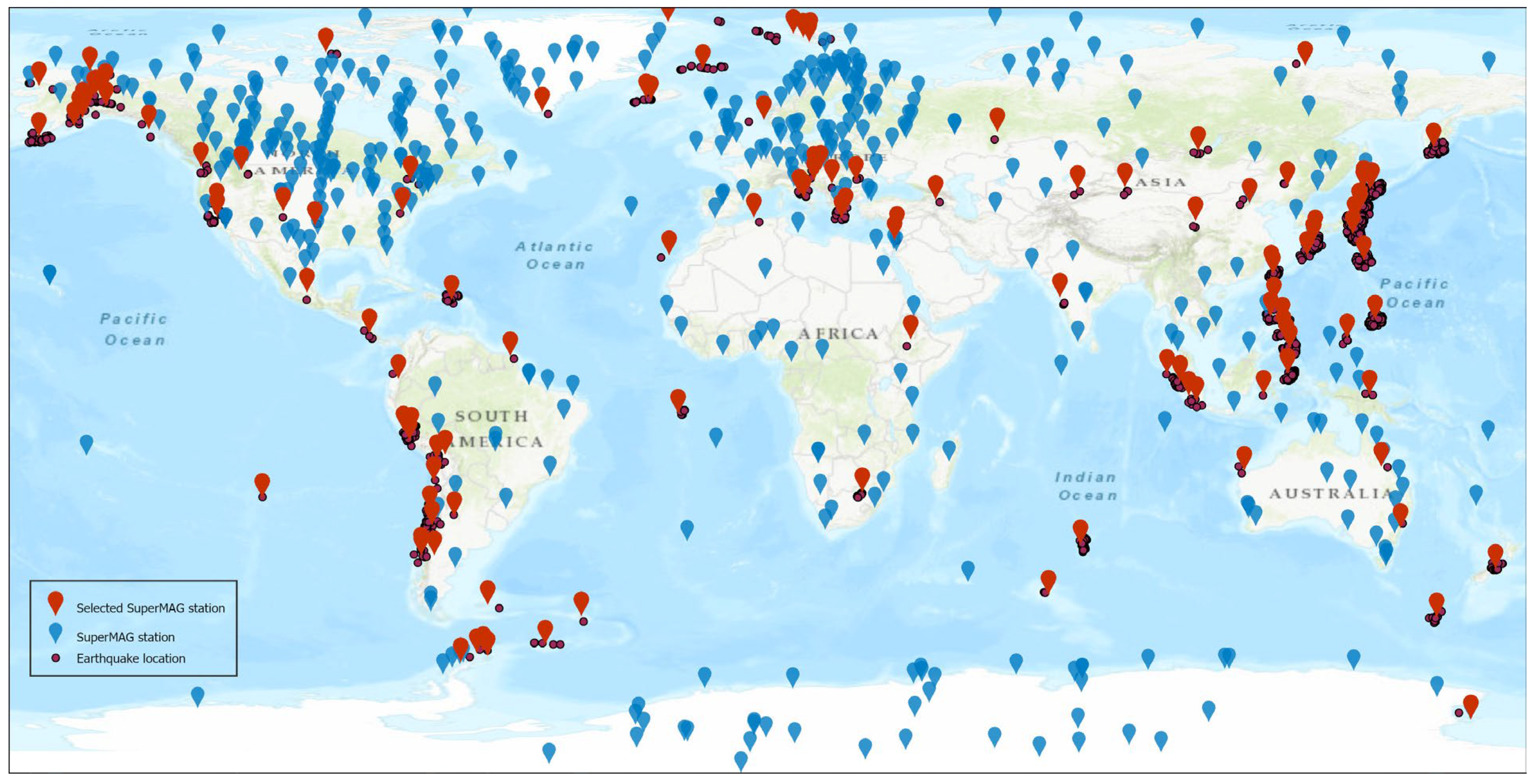
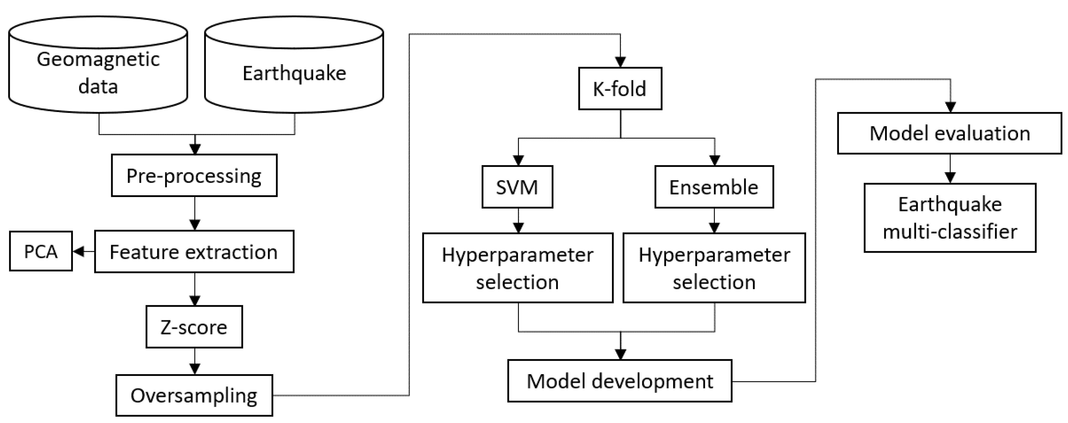
2. Data and Methods
3. Results and Discussion
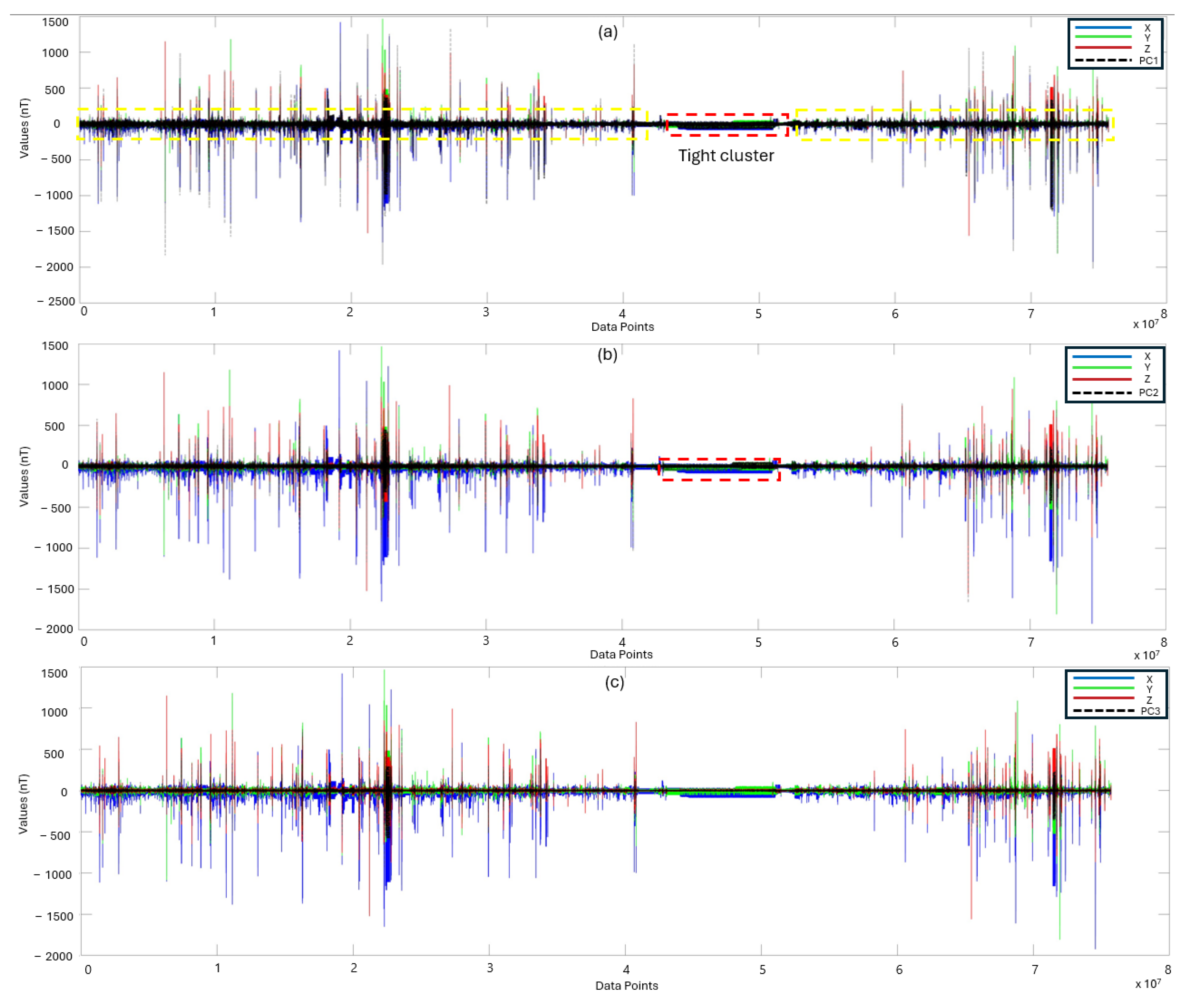
3.1. PCA Scores for Model Development
3.2. Hyperparameter Tuning and Algorithm Selection
3.3. Handling Imbalanced Data Using SMOTE
3.4. Ensemble Model Performance Based on PCA
4. Conclusions
Author Contributions
Funding
Data Availability Statement
Acknowledgments
Conflicts of Interest
References
- Wang, Z. Predicting or Forecasting Earthquakes and the Resulting Ground-Motion Hazards: A Dilemma for Earth Scientists. Seismol. Res. Lett. 2015, 86, 1–5. [Google Scholar] [CrossRef]
- Ghamry, E.; Mohamed, E.K.; Abdalzaher, M.S.; Elwekeil, M.; Marchetti, D.; de Santis, A.; Hegy, M.; Yoshikawa, A.; Fathy, A. Integrating Pre-Earthquake Signatures from Different Precursor Tools. IEEE Access 2021, 9, 33268–33283. [Google Scholar] [CrossRef]
- Han, R.; Cai, M.; Chen, T.; Yang, T.; Xu, L.; Xia, Q.; Jia, X.; Han, J. Preliminary Study on the Generating Mechanism of the Atmospheric Vertical Electric Field before Earthquakes. Appl. Sci. 2022, 12, 6896. [Google Scholar] [CrossRef]
- Yue, Y.; Koivula, H.; Bilker-Koivula, M.; Chen, Y.; Chen, F.; Chen, G. TEC Anomalies Detection for Qinghai and Yunnan Earthquakes on 21 May 2021. Remote Sens. 2022, 14, 4152. [Google Scholar] [CrossRef]
- Zöller, G.; Hainzl, S.; Tilmann, F.; Woith, H.; Dahm, T. Comment on “Potential short-term earthquake forecasting by farm animal monitoring” by Wikelski, Mueller, Scocco, Catorci, Desinov, Belyaev, Keim, Pohlmeier, Fechteler, and Mai. Ethology 2021, 127, 302–306. [Google Scholar] [CrossRef]
- Moro, M.; Saroli, M.; Stramondo, S.; Bignami, C.; Albano, M.; Falcucci, E.; Gori, S.; Doglioni, C.; Polcari, M.; Tallini, M.; et al. New insights into earthquake precursors from InSAR. Sci. Rep. 2017, 7, 12035. [Google Scholar] [CrossRef] [PubMed]
- Asaly, S.; Gottlieb, L.-A.; Inbar, N.; Reuveni, Y. Using Support Vector Machine (SVM) with GPS Ionospheric TEC Estimations to Potentially Predict Earthquake Events. Remote Sens. 2022, 14, 2822. [Google Scholar] [CrossRef]
- Hattori, K.; Han, P. Statistical Analysis and Assessment of Ultralow Frequency Magnetic Signals in Japan As Potential Earthquake Precursors: 13. In Pre-Earthquake Processes; American Geophysical Union (AGU): Washington, DC, USA, 2018; pp. 229–240. ISBN 9781119156949. [Google Scholar]
- Ouyang, X.-Y.; Parrot, M.; Bortnik, J. ULF Wave Activity Observed in the Nighttime Ionosphere above and Some Hours before Strong Earthquakes. J. Geophys. Res. Space Phys. 2020, 125, e2020JA028396. [Google Scholar] [CrossRef]
- Han, P.; Zhuang, J.; Hattori, K.; Chen, C.-H.; Febriani, F.; Chen, H.; Yoshino, C.; Yoshida, S. Assessing the Potential Earthquake Precursory Information in ULF Magnetic Data Recorded in Kanto, Japan during 2000–2010: Distance and Magnitude Dependences. Entropy 2020, 22, 859. [Google Scholar] [CrossRef]
- Asim, K.M.; Martínez-Álvarez, F.; Basit, A.; Iqbal, T. Earthquake magnitude prediction in Hindukush region using machine learning techniques. Nat. Hazards 2017, 85, 471–486. [Google Scholar] [CrossRef]
- Asim, K.M.; Idris, A.; Iqbal, T.; Martínez-Álvarez, F. Earthquake prediction model using support vector regressor and hybrid neural networks. PLoS ONE 2018, 13, e0199004. [Google Scholar] [CrossRef] [PubMed]
- Chang, X.; Zou, B.; Guo, J.; Zhu, G.; Li, W.; Li, W. One sliding PCA method to detect ionospheric anomalies before strong Earthquakes: Cases study of Qinghai, Honshu, Hotan and Nepal earthquakes. Adv. Space Res. 2017, 59, 2058–2070. [Google Scholar] [CrossRef]
- Gitis, V.G.; Derendyaev, A.B. Machine Learning Methods for Seismic Hazards Forecast. Geosciences 2019, 9, 308. [Google Scholar] [CrossRef]
- Debnath, P.; Chittora, P.; Chakrabarti, T.; Chakrabarti, P.; Leonowicz, Z.; Jasinski, M.; Gono, R.; Jasińska, E. Analysis of Earthquake Forecasting in India Using Supervised Machine Learning Classifiers. Sustainability 2021, 13, 971. [Google Scholar] [CrossRef]
- Arafa-Hamed, T.; Khalil, A.; Nawawi, M.; Marzouk, H.; Arifin, M. Geomagnetic Phenomena Observed by a Temporal Station at Ulu-Slim, Malaysia during The Storm of March 27, 2017. Sains Malays. 2019, 48, 2427–2435. [Google Scholar] [CrossRef]
- Chen, B.H. Minimum standards for evaluating machine-learned models of high-dimensional data. Front. Aging 2022, 3, 901841. [Google Scholar] [CrossRef] [PubMed]
- Liu, Y.; Yong, S.; He, C.; Wang, X.; Bao, Z.; Xie, J.; Zhang, X. An Earthquake Forecast Model Based on Multi-Station PCA Algorithm. Appl. Sci. 2022, 12, 3311. [Google Scholar] [CrossRef]
- Li, J.; Li, Q.; Yang, D.; Wang, X.; Hong, D.; He, K. Principal Component Analysis of Geomagnetic Data for the Panzhihua Earthquake (Ms 6.1) in August 2008. Data Sci. J. 2011, 10, IAGA130–IAGA138. [Google Scholar] [CrossRef]
- Hattori, K.; Serita, A.; Gotoh, K.; Yoshino, C.; Harada, M.; Isezaki, N.; Hayakawa, M. ULF geomagnetic anomaly associated with 2000 Izu Islands earthquake swarm, Japan. Phys. Chem. Earth Parts A/B/C 2004, 29, 425–435. [Google Scholar] [CrossRef]
- Fernández-Gómez, M.; Asencio-Cortés, G.; Troncoso, A.; Martínez-Álvarez, F. Large Earthquake Magnitude Prediction in Chile with Imbalanced Classifiers and Ensemble Learning. Appl. Sci. 2017, 7, 625. [Google Scholar] [CrossRef]
- Mukherjee, S.; Gupta, P.; Sagar, P.; Varshney, N.; Chhetri, M. A Novel Ensemble Earthquake Prediction Method (EEPM) by Combining Parameters and Precursors. J. Sens. 2022, 5321530. [Google Scholar] [CrossRef]
- SuperMAG Database. Available online: https://supermag.jhuapl.edu/ (accessed on 9 October 2023).
- United States Geological Survey (USGS) Database. Available online: www.earthquake.usgs.gov (accessed on 9 October 2023).
- Yusof, K.A.; Abdullah, M.; Hamid, N.S.A.; Ahadi, S.; Ghamry, E. Statistical Global Investigation of Pre-Earthquake Anomalous Geomagnetic Diurnal Variation Using Superposed Epoch Analysis. IEEE Trans. Geosci. Remote Sens. 2022, 60, 1–13. [Google Scholar] [CrossRef]
- Yusof, K.A.; Mashohor, S.; Abdullah, M.; Rahman, M.A.A.; Hamid, N.S.A.; Qaedi, K.; Matori, K.A.; Hayakawa, M. Earthquake Prediction Model Based on Geomagnetic Field Data Using Automated Machine Learning. IEEE Geosci. Remote Sens. Lett. 2024, 21, 1–5. [Google Scholar] [CrossRef]
- Ismail, N.H.; Ahmad, N.; Mohamed, N.A.; Tahar, M.R. Analysis of Geomagnetic Ap Index on Worldwide Earthquake Occurrence using the Principal Component Analysis and Hierarchical Cluster Analysis. Sains Malays. 2021, 50, 1157–1164. [Google Scholar] [CrossRef]
- Xu, G.; Han, P.; Huang, Q.; Hattori, K.; Febriani, F.; Yamaguchi, H. Anomalous behaviors of geomagnetic diurnal variations prior to the 2011 off the Pacific coast of Tohoku earthquake (Mw9.0). J. Asian Earth Sci. 2013, 77, 59–65. [Google Scholar] [CrossRef]
- Alvarez, D.A.; Hurtado, J.E.; Bedoya-Ruíz, D.A. Prediction of modified Mercalli intensity from PGA, PGV, moment magnitude, and epicentral distance using several nonlinear statistical algorithms. J. Seismol. 2012, 16, 489–511. [Google Scholar] [CrossRef]
- Elreedy, D.; Atiya, A.F. A Comprehensive Analysis of Synthetic Minority Oversampling Technique (SMOTE) for handling class imbalance. Inf. Sci. 2019, 505, 32–64. [Google Scholar] [CrossRef]
- Bao, Z.; Zhao, J.; Huang, P.; Yong, S.; Wang, X. A Deep Learning-Based Electromagnetic Signal for Earthquake Magnitude Prediction. Sensors 2021, 21, 4434. [Google Scholar] [CrossRef]
- Cui, S.; Yin, Y.; Wang, D.; Li, Z.; Wang, Y. A stacking-based ensemble learning method for earthquake casualty prediction. Appl. Soft Comput. 2021, 101, 107038. [Google Scholar] [CrossRef]


| X (nT) | Y (nT) | Z (nT) | PC1 (nT) | PC2 (nT) | PC3 (nT) | |
|---|---|---|---|---|---|---|
| Mean | 8.24 | −0.35 | 1.46 | 7.33 × 10⁻⁸ | −5.80 × 10⁻⁹ | 4.14 × 10⁻⁸ |
| Median | −4.75 | −0.10 | 1.21 | 1.13 | −0.09 | 0.02 |
| Variance | 624.26 | 132.58 | 169.87 | 598.34 | 138.28 | 52.12 |
| Standard deviation | 24.98 | 11.51 | 13.03 | 24.46 | 11.75 | 7.21 |
| Range | 3343.75 | 3275.55 | 2711.71 | 3352.75 | 2429.60 | 1670.76 |
| Min | −1924.85 | −1809.16 | −1561.00 | −2017.81 | −1660.95 | −926.62 |
| Max | 1418.90 | 1466.38 | 1150.70 | 1334.93 | 768.65 | 744.13 |
| SVM Hyperparameter | SVM | Ensemble Hyperparameter | Ensemble |
|---|---|---|---|
| Kernel function | Gaussian | Method | bagging |
| Box constraint | 50 | Num of learners | 200 |
| Kernel | 0.5 | Split size | 13,000 |
| Nu | 0.01 | Leaf size | 0.01 |
| Predictor selection | curvature |
| Model | SVM | Ensemble |
|---|---|---|
| Accuracy | 75.88% | 77.50% |
| Sensitivity | 75.88% | 77.50% |
| Specificity | 96.55% | 96.79% |
| Precision | 77.56% | 76.69% |
| F1-score | 76.16% | 77.05% |
| MCC | 73.11% | 73.88% |
Disclaimer/Publisher’s Note: The statements, opinions and data contained in all publications are solely those of the individual author(s) and contributor(s) and not of MDPI and/or the editor(s). MDPI and/or the editor(s) disclaim responsibility for any injury to people or property resulting from any ideas, methods, instructions or products referred to in the content. |
© 2024 by the authors. Licensee MDPI, Basel, Switzerland. This article is an open access article distributed under the terms and conditions of the Creative Commons Attribution (CC BY) license (https://creativecommons.org/licenses/by/4.0/).
Share and Cite
Qaedi, K.; Abdullah, M.; Yusof, K.A.; Hayakawa, M. Feasibility of Principal Component Analysis for Multi-Class Earthquake Prediction Machine Learning Model Utilizing Geomagnetic Field Data. Geosciences 2024, 14, 121. https://doi.org/10.3390/geosciences14050121
Qaedi K, Abdullah M, Yusof KA, Hayakawa M. Feasibility of Principal Component Analysis for Multi-Class Earthquake Prediction Machine Learning Model Utilizing Geomagnetic Field Data. Geosciences. 2024; 14(5):121. https://doi.org/10.3390/geosciences14050121
Chicago/Turabian StyleQaedi, Kasyful, Mardina Abdullah, Khairul Adib Yusof, and Masashi Hayakawa. 2024. "Feasibility of Principal Component Analysis for Multi-Class Earthquake Prediction Machine Learning Model Utilizing Geomagnetic Field Data" Geosciences 14, no. 5: 121. https://doi.org/10.3390/geosciences14050121
APA StyleQaedi, K., Abdullah, M., Yusof, K. A., & Hayakawa, M. (2024). Feasibility of Principal Component Analysis for Multi-Class Earthquake Prediction Machine Learning Model Utilizing Geomagnetic Field Data. Geosciences, 14(5), 121. https://doi.org/10.3390/geosciences14050121