Hazard and Risk-Based Tsunami Early Warning Algorithms for Ocean Bottom Sensor S-Net System in Tohoku, Japan, Using Sequential Multiple Linear Regression

Abstract

This study presents robust algorithms for tsunami early warning using synthetic tsunami wave data at ocean bottom sensor (OBS) arrays with sequential multiple linear regression. The study focuses on the Tohoku region of Japan, where an S-net OBS system (150 pressure sensors) has been deployed. To calibrate the tsunami early warning system using realistic tsunami wave profiles at the S-net stations, 4000 stochastic tsunami simulations are employed. Forecasting models are built using multiple linear regression together with sequential feature selection based on Akaike Information Criterion and knee-point method to identify sensors that improve the accuracy most significantly. The study considers tsunami wave amplitude at a nearshore location and regional tsunami loss for buildings to develop hazard-based and risk-based tsunami warning algorithms. The models identify an optimal configuration of OBS stations and waiting time for issuing tsunami warnings. The model performance is compared against a base model, which only uses the earthquake magnitude and epicenter location. The result indicates that estimating the tsunami amplitude and loss via S-net improves accuracy. For the hazard-based forecasting, adding six sensors from the S-net improves the accuracy of the estimation most significantly with an optimal waiting time of 3 min. For the risk-based forecasting, a longer waiting time between 5 and 10 min is suitable.

1. Introduction

A tsunami can cause great destruction to a coastal region by damaging buildings and infrastructure and by depriving people’s lives. Taking the 2011 Tohoku tsunami in Japan as an example, it was generated by a moment magnitude (M) 9.0 earthquake and recorded a high run-up of 40+ m in Miyako [1]. The impact of the 2011 Tohoku earthquake and tsunami on coastal communities was tremendous and even caused a serious accident at Fukushima Daiichi Nuclear Power Plant [2]. The total death tolls were over 19,700 people, and the damage costs exceeded USD 170 billion [3,4]. Although tsunamis cannot be prevented, their severe impact can be mitigated through enhanced tsunami preparedness, timely warning, and effective response [5,6]. Therefore, the tsunami early warning system is an effective tool to reduce victims [7,8,9].

The Japan Meteorological Agency (JMA) is responsible for forecasting and issuing warnings that relate to earthquake and tsunami threats in Japan. JMA originally used an automatic monitoring method to estimate the earthquake magnitude and epicenter location and to forecast the impact of earthquakes and tsunamis. During the 2011 Tohoku tsunami, JMA was unable to forecast the tsunami triggered by this large earthquake of M9.0 using the original JMA method [10]. The inaccuracy was due to the underestimation of the earthquake magnitude caused by saturation of seismic signals, and as a result, the tsunami waves were initially underpredicted, and the tsunami warning update was too late [11].

To improve the accuracy of tsunami forecasting and early warning, JMA proposed to use more ocean bottom sensors (OBS) and increase the number of off-shore sensors in the ocean. The S-net project started in 2011 [12,13], involving a large network of submarine seismic and tsunami sensors around Japan Trench. The S-net has 150 real-time monitoring pressure sensors (tsunami meters) in total, which cover an area of 1000 × 300 km² from off-Hokkaido to off-Kanto [14]. The accuracy of tsunami forecasting depends on how the S-net sensors are geographically located [5,6].

In calibrating a robust tsunami early warning system, it is important that the system is tested to work well for a variety of possible earthquake ruptures. However, there is no abundant historical tsunami data that can be directly used for developing such a warning system, because no major tsunami events occurred since the 2011 Tohoku tsunami. As it is uncertain how the future tsunami events may unfold, it is sensible to use synthetic tsunami wave data to calibrate a tsunami early warning algorithm based on conventional earthquake source information (e.g., JMA’s magnitude estimate and epicenter location) as well as S-net wave data. For this purpose, adopting stochastic tsunami simulation models that are developed for the Tohoku region [15,16] is a suitable approach. The stochastic tsunami simulations facilitate the consideration of realistic heterogeneous earthquake slips, which are seismologically and statistically compatible with inferred earthquake slips via source inversion analyses (e.g., [17]). Once a large set of synthetic earthquake source models is simulated, wave profiles at off-shore and some coastal locations can be generated by evaluating physics-based governing equations, which capture both spatial and temporal resolutions. Subsequently, coastal tsunami inundation can be simulated, and the corresponding regional tsunami loss for buildings can be calculated by using suitable exposure and fragility models [18]. This numerical set-up is particularly useful because it facilitates the development of tsunami early warning algorithms for not only conventional hazard metrics (the probability of occurrence of the tsunami event, which is quantified by wave amplitude at a shallow coastal location near a town/city) but also risk metrics (the product of hazard, exposure, and vulnerability, which is quantified by the total tsunami loss of damaged buildings in coastal communities).

This study presents new effective and robust algorithms for tsunami early warning using synthetic tsunami wave data at S-net OBS arrays with sequential multiple linear regression (MLR). The calibration data are generated through stochastic tsunami simulations that have been carried out for the Tohoku region of Japan by considering the 2011 Tohoku tsunami hazard and risk data [15,16,18]. Two types of forecasting models are developed: the hazard-based warning system uses tsunami wave amplitude at a nearshore location, whereas the risk-based warning system adopts regional tsunami loss of buildings along the coast. For both hazard- and risk-based warning algorithms, an optimal configuration of OBS stations and waiting time for issuing tsunami warnings are identified by implementing sequential MLR together with Akaike Information Criterion (AIC) [19] and knee-point method [20]. The model performance is compared against a base model, which only uses the earthquake magnitude and epicenter location. The identification of a more compact OBS network system for tsunami early warning is motivated because the installation and maintenance of the off-shore sensors are expensive [21], and a smaller network of stations can be more easily deployed [22]. In such a system, the waiting time should be relatively short, since a trade-off exists between data acquisition time and evacuation time [23,24]. One of the important conclusions that this paper aims to draw is to demonstrate that the forecasting performance is improved by using tsunami data from the S-net, in comparison with the conventional forecasting method based on earthquake information alone. The novelty of this work includes: (i) a comprehensive set of stochastic tsunami simulation results is adopted for developing tsunami early warning systems for the S-net; (ii) risk-based tsunami warning approaches are investigated; and (iii) optimal networks for different forecasting metrics are obtained through extensive statistical analyses.

2. Tsunami Simulation Data and Forecasting Methods

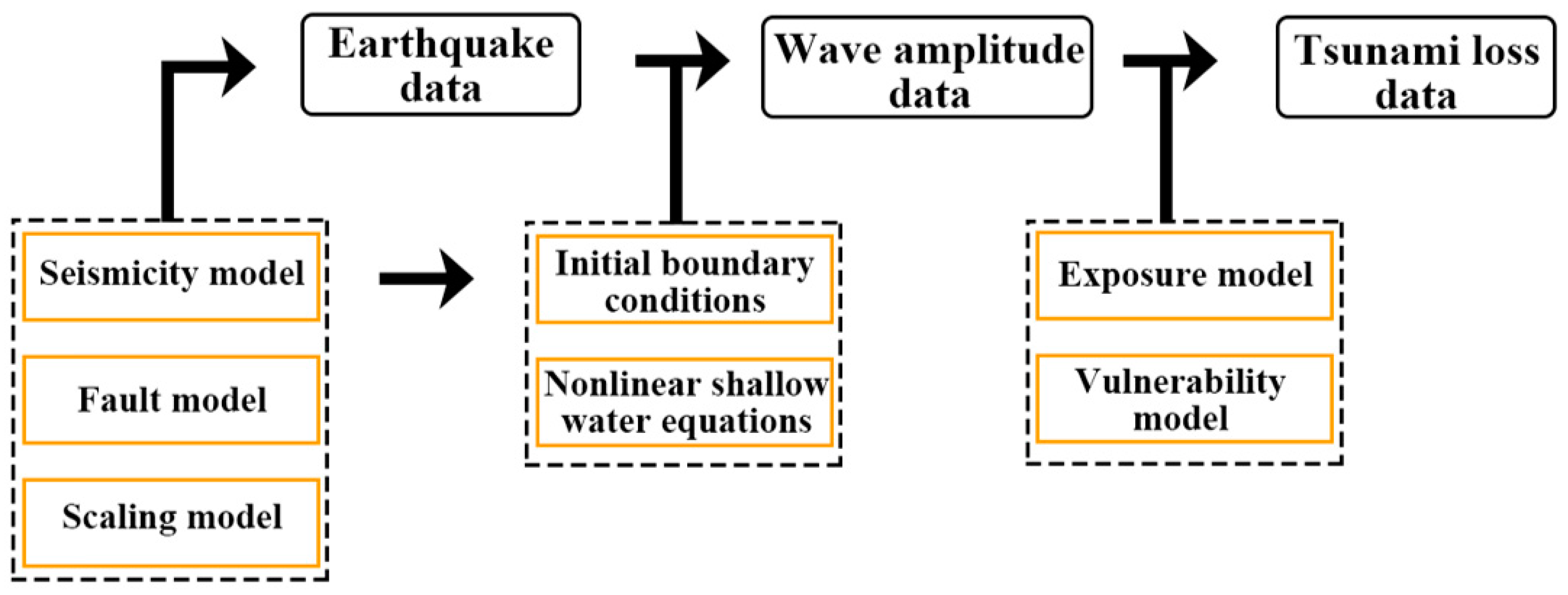
2.1. Tsunami Simulation Data

Hypothetical data, obtained from numerical tsunami simulations, are commonly used in tsunami scenarios [25,26,27,28,29]. Because historical events of earthquakes and tsunamis are lacking to perform statistical analyses, 4000 cases of simulated stochastic earthquakes are used in this study, although there is a tsunami event during the 2016 Fukushima earthquake [30]. The processes of how the data used in this study are generated are shown in Figure 1. The earthquake data, including magnitude, epicenter, and earthquake slip, are first simulated from the seismicity, fault, and scaling models [16]. Then, by solving nonlinear shallow water equations for given initial dislocation profiles of water, wave amplitude data are generated at selected recording locations (e.g., S-net stations and nearshore coastal locations). After simulating the inundation heights at building locations, the tsunami loss is evaluated by integrating hazard, exposure, and vulnerability models [18]. In the context of this study, the maximum on-shore tsunami amplitude is used as a response variable for the hazard-based early warning system, whereas the portfolio tsunami loss from buildings is adopted as a response variable for the risk-based system. Explanatory variables of the early warning system are the earthquake source information (i.e., magnitude and epicenter location) and the wave amplitude at the off-shore S-net sensor locations.

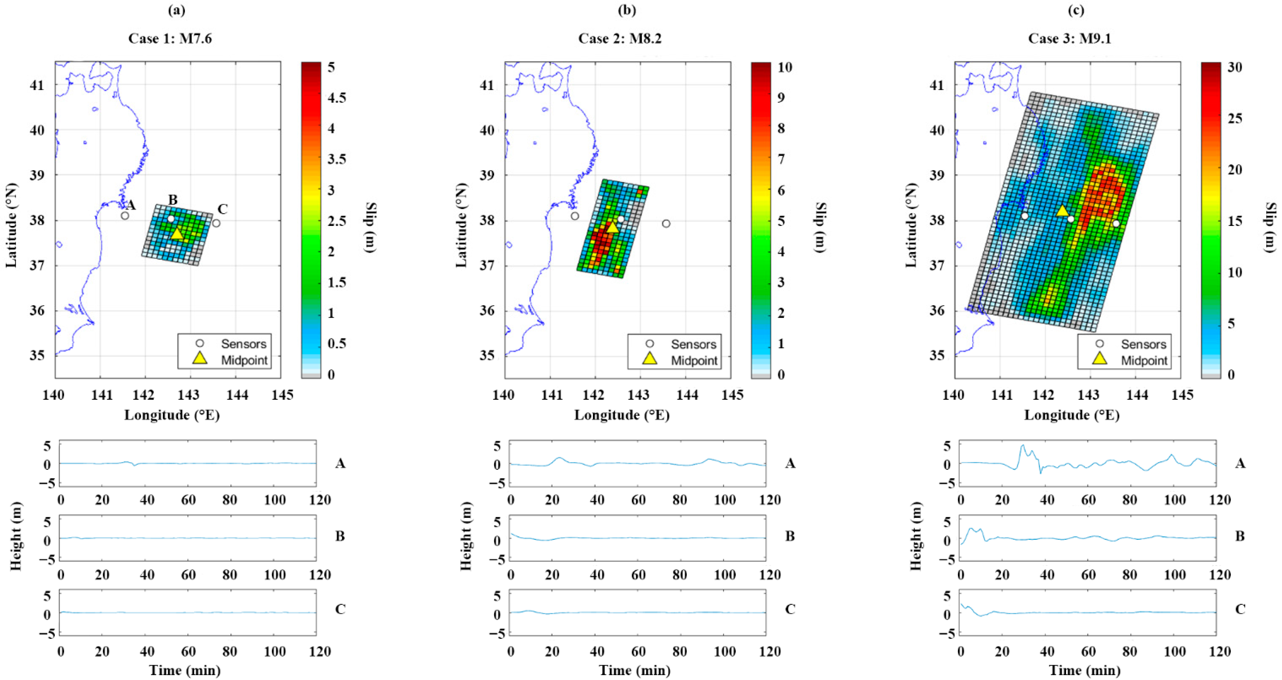
2.1.1. Stochastic Earthquakes

The stochastic tsunami simulations can be used to generate earthquake rupture models for future events [16]. The seismicity model (e.g., a statistical earthquake occurrence-magnitude model based on earthquake catalog data in the Tohoku region) characterizes the distribution of earthquakes. Figure 2 shows the two interested locations, Iwanuma and Onagawa, with their building asset distributions (see Figure 2a) and the 99 off-shore sensors that measure the wave amplitude (Figure 2b). The regional fault source model represents the 2011 Tohoku earthquake fault plane, covering an area spanning 650 km long and 250 km wide [31]. The earthquake source zone is discretized into 10 × 10 km² sub-fault areas (see Figure 3a) to achieve heterogeneous slips. Eight source parameters, including fault length, fault width, mean slip, maximum slip, Box-Cox power parameter, correlation length along dip, correlation length along strike, and Hurst number, are used to determine the size, position, and slip distribution of the earthquakes [16]. The whole range of the simulated earthquake magnitudes is from M7.5 to M9.1, with 0.2 bin width, the 4000 cases of earthquake ruptures are evenly split into eight classes (the first class contains 500 cases of earthquake within M7.5–M7.7, while the eighth class contains 500 cases of earthquake within M8.9–M9.1). The earthquake magnitude is used as a fundamental explanatory variable to forecast major tsunami wave arrivals since both maximum on-shore tsunami amplitude and tsunami loss have an increasing trend with it (see Figure 4 and Figure 5). However, the variability of tsunami amplitude and loss is still large for a specific magnitude range. Additional information is necessary to achieve a robust forecasting.

2.1.2. Wave Amplitude

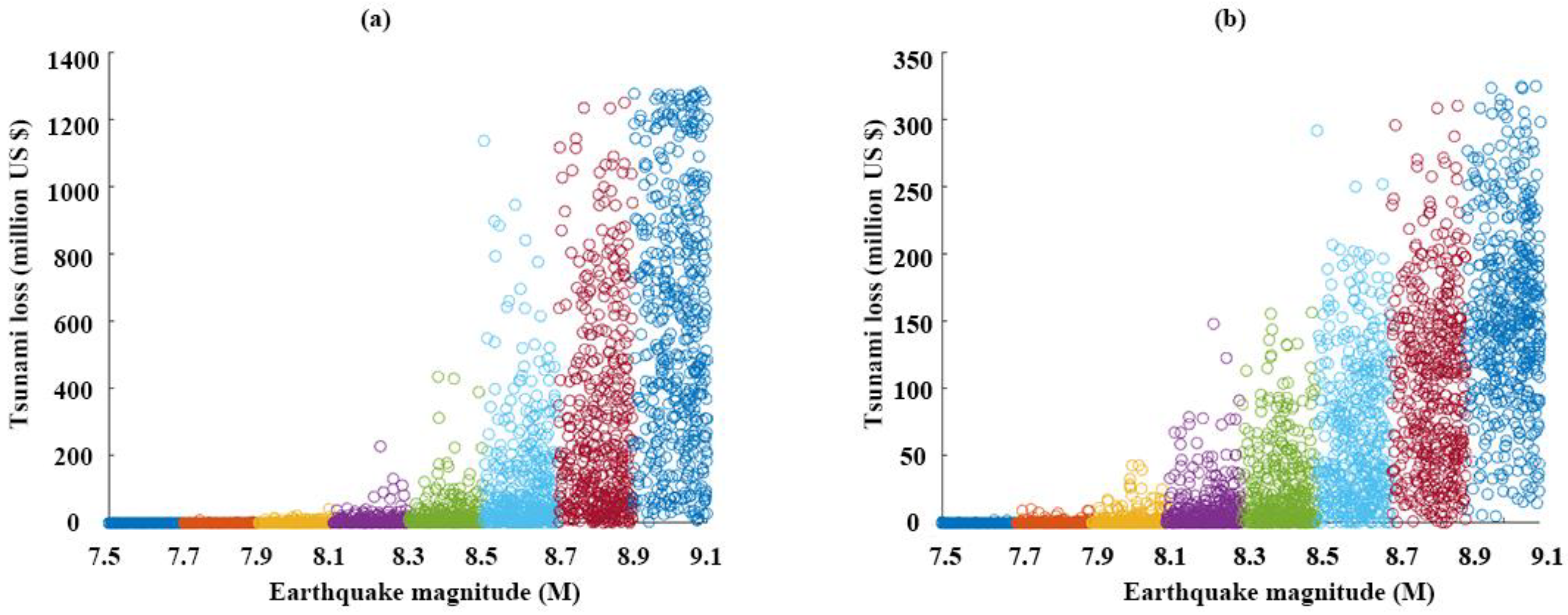
The wave amplitude data can be used as both the response variable, i.e., maximum amplitude at the interested locations, and the explanatory variable, i.e., wave amplitude at off-shore S-net locations (Figure 2). A well-tested TSUNAMI computer code [32] is used to generate the tsunami wave amplitude by solving nonlinear shallow water equations, which provide both spatial and temporal resolutions. The initial water surface elevation was estimated using formulae by Okada [33] and Tanioka and Satake [34]; the latter is considered to account for the effects of horizontal deformation of the seafloor in the accretionary prism of the subduction areas. A complete dataset of bathymetry/elevation, coastal/riverside structures, and surface roughness, provided by the Miyagi Prefectural Government, is organized into nesting grids of four resolutions (i.e., 1350-m, 450-m, 150-m and 50-m domains). In the tsunami simulation, the coastal/riverside structures are represented by a vertical wall at one or two sides of the computational cells. To evaluate the volume of water that overpasses these walls, Honma’s weir formulae are employed [35]. The bottom friction is evaluated using Manning’s formula following the Japan Society of Civil Engineers standard [35]. The simulation of the wave amplitude starts when an earthquake rupture is initiated, and the duration is set to 120 min [18].

Figure 3 shows three different earthquake scenarios and waveforms at three selected locations. The farther the off-shore sensors are from the coastline, the earlier they can detect the wave arrivals. The off-shore sensors contain useful information for calibrating the warning algorithm. Figure 4 shows the plot of the maximum on-shore tsunami amplitude against earthquake magnitude in Iwanuma and Onagawa. The average tsunami amplitude increases as the earthquake magnitude increases. The high magnitude earthquakes determine the tsunami, and the earthquake information can be used as a fundamental factor for the tsunami early warning. However, the variation of tsunami amplitude is significant among different earthquake magnitudes, and the earthquake magnitude may not be the most suitable feature to forecast the tsunami amplitude. Wave amplitude collected by the off-shore sensors may be more suitable for forecasting the tsunami amplitude for tsunami early warning purposes.

2.1.3. Tsunami Loss

After the wave data are generated, inundation depths at building locations (Figure 2) are estimated, and tsunami damage of these buildings is evaluated by applying the tsunami fragility functions. More specifically, the tsunami fragility model [36] is implemented to evaluate the probability of different severities of tsunami damage as a function of inundation depth. Using Monte Carlo simulations, tsunami damage states are determined, and then, tsunami loss is evaluated by considering the following damage ratios: minor (0.03–0.1), moderate (0.1–0.3), extensive (0.3–0.5), complete (0.5–1.0), and collapse (1.0). For a damage state with lower and upper limits (e.g., the moderate damage state is specified with damage ratios between 0.1 and 0.3), a damage ratio is sampled from a uniform distribution. The exposure model includes the portfolio of 6152 and 1760 building assets near the coastline in Iwanuma and Onagawa, respectively. The building dataset is based on the post-2011-Tohoku tsunami damage data compiled by the Ministry of Land Infrastructure and Transportation. The building data include information of the building location, structural material, and number of stories, which can be used to estimate the cost of buildings. Finally, tsunami loss is calculated by sampling a value of the total replacement cost for a building from the lognormal distribution and then by multiplying it by the final damage ratio [18].

Figure 5 shows the tsunami loss against earthquake magnitude in Iwanuma and Onagawa. Since Iwanuma has about three times more building assets than Onagawa, the building loss in Iwanuma tends to be higher than the loss in Onagawa. The tsunami loss starts to increase when the earthquake magnitude is over M7.9 and increases significantly when the magnitude exceeds M8.5. It is noteworthy that the variability of the tsunami loss is large, even larger than the tsunami amplitude. This means that a tsunami triggered by a large magnitude earthquake has high potential to cause a large loss, but it is difficult to predict the exact loss value due to its large uncertainty by using earthquake magnitude alone. Thus, it is important to investigate whether the use of off-shore sensors can help forecast the tsunami loss more accurately and issue a more accurate tsunami early warning based on this risk metric.

The tsunami loss is a rare event even when the earthquake magnitude is relatively large, and the positions of large earthquake slips with respect to the target city/town location have significant influence on the tsunami loss. In other words, the directivity of tsunami waves is an important factor in forecasting potential tsunami consequences. To visualize this effect clearly, Figure 6 plots the earthquake magnitude and the earthquake latitude by distinguishing tsunami loss cases and no tsunami loss cases. The plots show a separation of with-loss and without-loss cases in a fan-shaped manner with its origin corresponding to the target location of the town. The fan-shaped spread of the non-zero tsunami loss data for Iwanuma is wider than that for Onagawa. Since the logarithmic transformation is applied to the loss data to reduce the skewness in the loss data, non-zero tsunami loss data are employed in the MLR analyses (see Section 2.2). It is noted that these non-zero tsunami loss data can be distinguished effectively by implementing logistic regression using earthquake magnitude and latitude differences with respect to the target location.

2.2. Methods

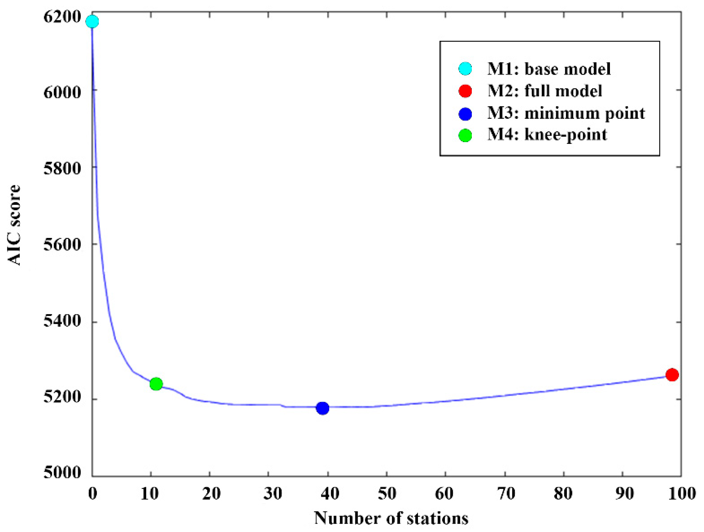
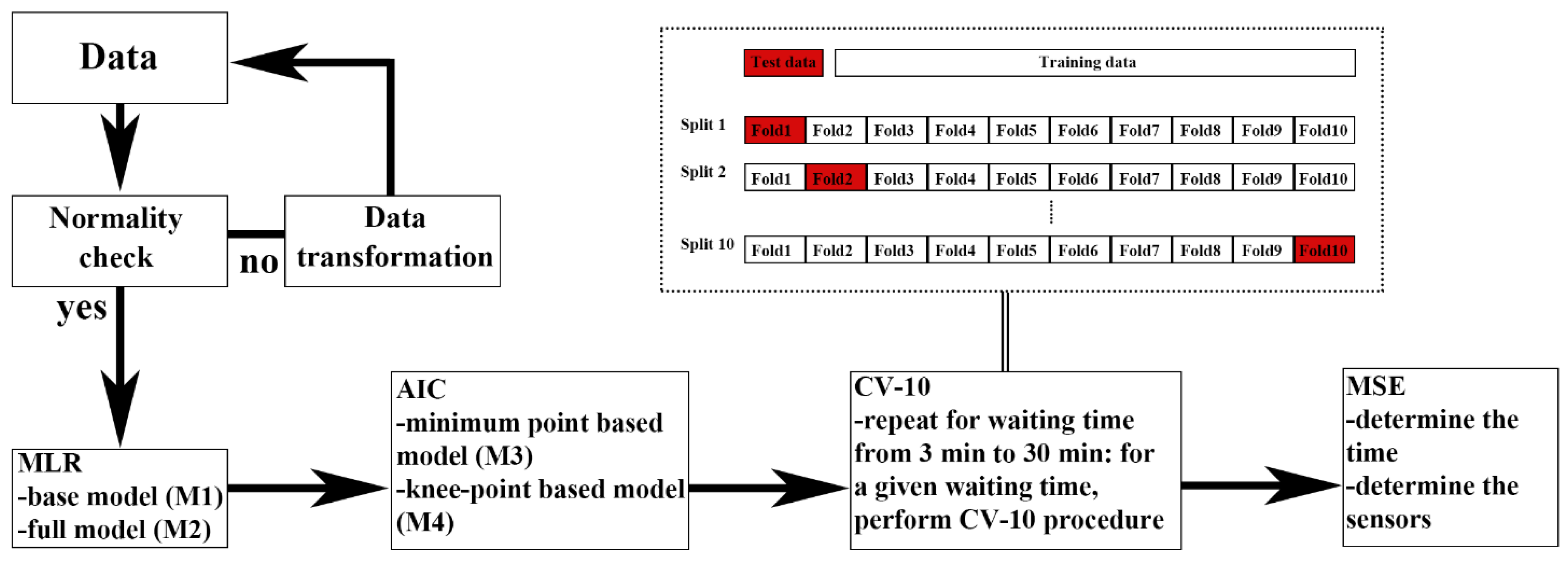
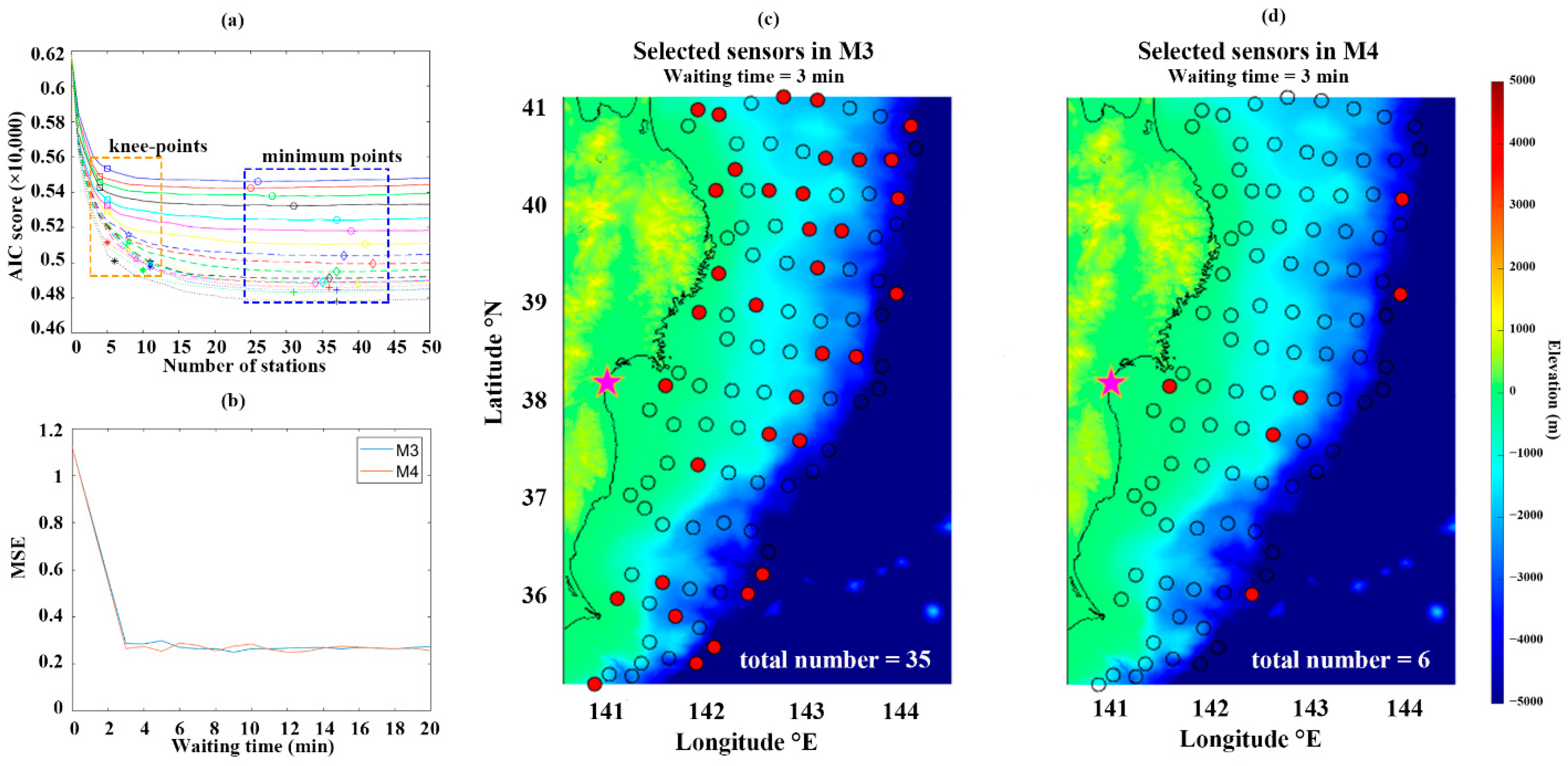
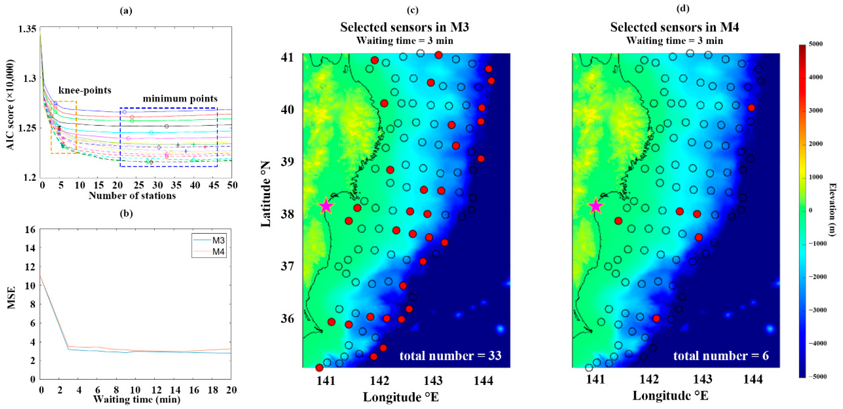
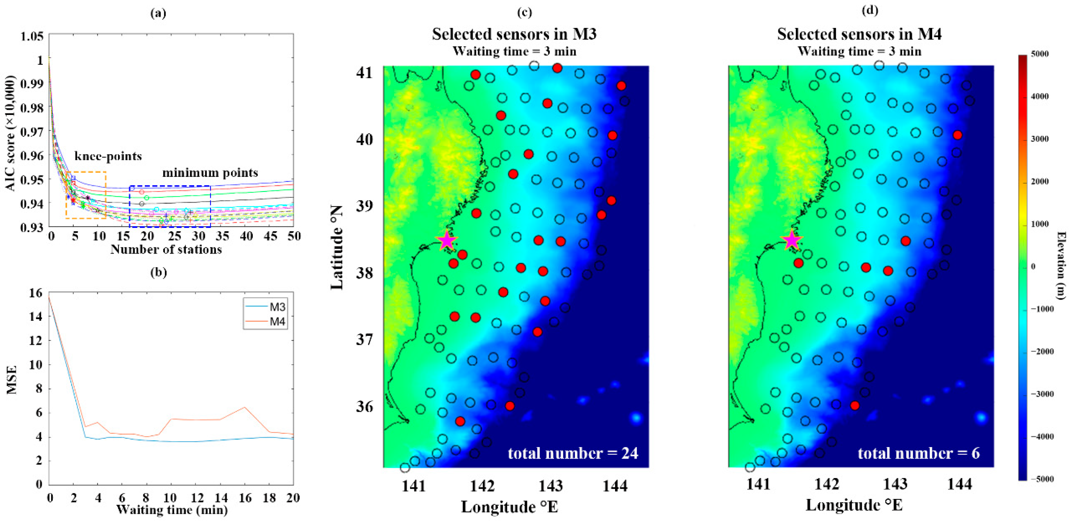
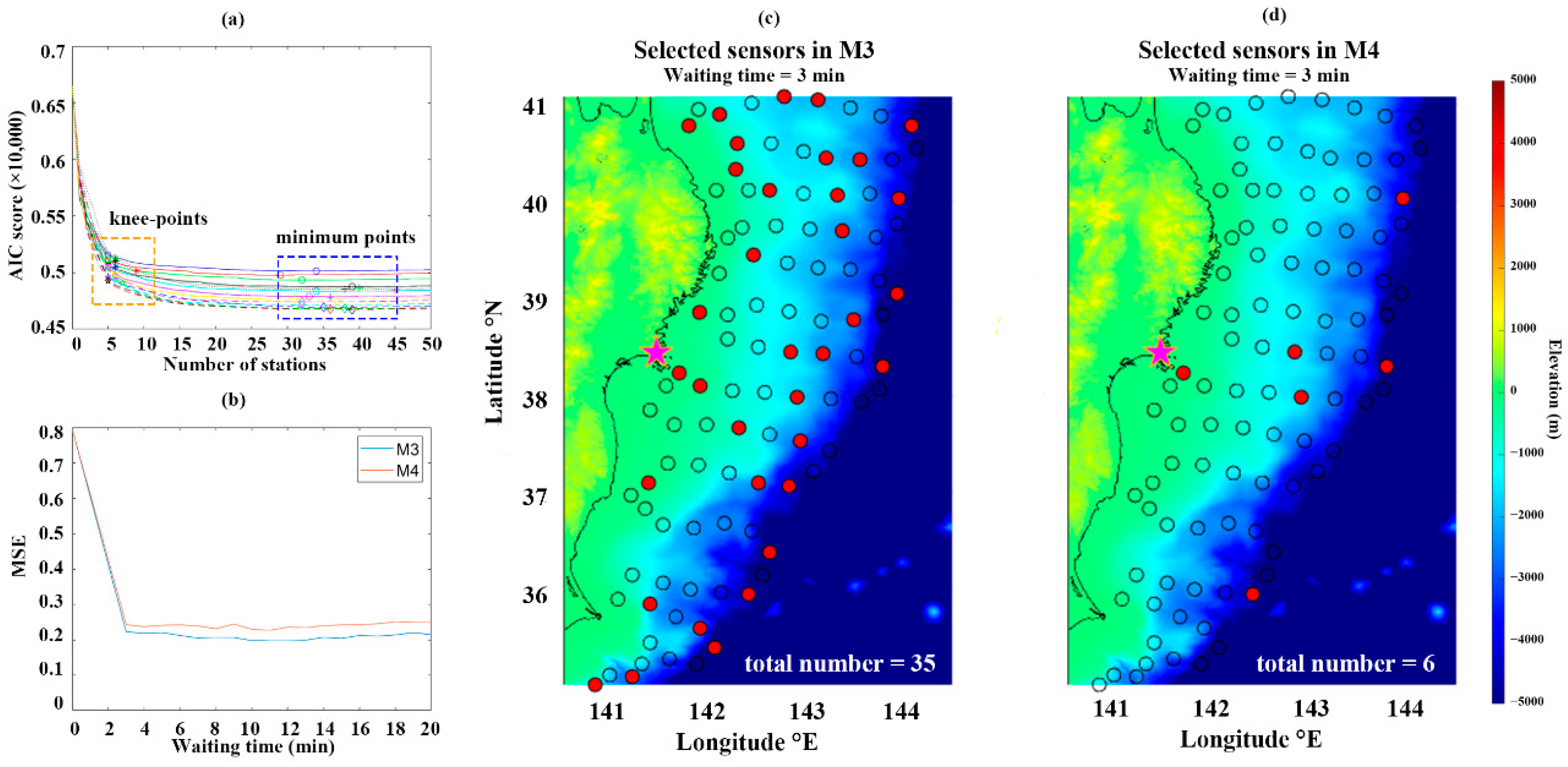
2.2.1. Multiple Linear Regression with AIC Forward Selection and Knee-Point

MLR is a linear regression model that uses two or more explanatory variables to predict the response variable. The response variables in this study are the maximum on-shore tsunami amplitude and the tsunami loss (see Figure 4 and Figure 5). The explanatory variables are earthquake magnitude ($x_{mag}$), earthquake latitude ($x_{lat}$), earthquake longitude ($x_{long}$), and the maximum wave amplitude collected at the $i$ off-shore sensors during a specific waiting time, where $i=1,2,\dots ,99$. The base (M1) and full (M2) models can be written as:

$$M1={\beta }_0+x_{mag}{\beta }_{mag}+x_{lat}{\beta }_{lat}+x_{long}{\beta }_{long}$$

(1)

$$M2={\beta }_0+x_{mag}{\beta }_{mag}+x_{lat}{\beta }_{lat}+x_{long}{\beta }_{long}+{\displaystyle \sum }_{i=1}^{99}{x}_i{\beta }_i$$

(2)

Since the distribution of the data is assumed to be normal in MLR, logarithmic transformation is applied to the response variables to reduce the skewness of the data. Non-zero tsunami loss data are used for calibrating the risk-based tsunami early warning model (Figure 6).

Since there are 102 explanatory variables (3 earthquake parameters plus 99 off-shore sensor parameters) in the full model, the variable reduction is needed to remove redundant variables to avoid collinearity in MLR and to identify the most informative off-shore sensors. After the MLR model is fitted, variable selection using AIC and knee-point are applied to select the most informative variables. In this study, the earthquake information is kept in the model, since using the earthquake information is a standard approach to issue early warning [37,38], and this information is usually available a few minutes after an earthquake. The variable selection is applied to the 99 off-shore sensors, so that a smaller number of informative off-shore sensors can be defined. AIC is an estimator of prediction error and accounts for the trade-off between the goodness-of-fit and the simplicity of the model. The lower the AIC value is, the better the model is. AIC uses the likelihood ratio to estimate the goodness-of-fit of each model and gives a penalty when more explanatory variables are used [19]. Denoting the number of parameters in the model by $k$, the total number of observations by $n$, and the maximum likelihood estimator (MLE) by $\widehat{\theta }$, the formula of AIC can be written as:

$$AIC=-2\log \left(\widehat{\theta }\right)+2k$$

(3)

$\widehat{\theta }$ is calculated as by maximizing the loglikelihood L:

$$L\left(\mu ,\sigma |x_1,x_2,\dots ,x_n\right)={\displaystyle \prod }_{i=1}^{n}L\left(\mu ,\sigma |x_i\right)={\displaystyle \prod }_{i=1}^n\frac{1}{\sqrt{2\pi {\sigma }^2}}{e}^{-\frac{{(x_i-\mu )}^2}{2{\sigma }^2}}$$

(4)

The forward selection is a method of stepwise regression that starts with the base model and adds a variable that improves the most for the model one by one. The AIC value of the base model usually is large when the forward selection procedure is initiated, and as more variables are added to the model, the AIC value will decrease rapidly, reach a minimum value, and then increase when enough parameters are added. The knee-point method has been widely used in the optimal selection problem [20,39,40]. This method is useful for identifying an effective early warning system with a minimum number of sensors. The model equation for the minimum AIC can be written as:

$$M3={\beta }_0+x_{mag}{\beta }_{mag}+x_{lat}{\beta }_{lat}+x_{long}{\beta }_{long}+{\displaystyle \sum }_{i=1}^{k1}{x}_i{\beta }_i$$

(5)

Whereas the model equation for the knee-point based model can be written as:

$$M4={\beta }_0+x_{mag}{\beta }_{mag}+x_{lat}{\beta }_{lat}+x_{long}{\beta }_{long}+{\displaystyle \sum }_{i=1}^{k2}{x}_i{\beta }_i$$

(6)

where 0 < $k2$ < $k1$ < 99.

Figure 7 shows an example of knee-point and minimum points. The trend of the AIC score decreases significantly from the base model (M1) to the model based on the knee-point method (M4), slowly decreases to the minimum point (M3), and increases slightly to the end (M2). The corresponding numbers of sensors that are picked by the minimum point and the knee-point are used to fit the model. The knee-point method with a smaller number of off-shore sensors provides a relatively good prediction, whereas the minimum method provides the optimal selection based on AIC scores. The model performances of M1, M2, M3 and M4 are compared for both hazard-based and risk-based analyses for Iwanuma and Onagawa. The most informative number of off-shore sensors and optimal waiting time are identified based on the model performances.

2.2.2. Comparison of Model Performances

The process of how to fit and compare the models is shown in Figure 8. In Section 2.2.1, for a given waiting time (e.g., for 5 min waiting time, x_i represents the maximum wave amplitude up to 5 min at the ith station), the process of developing M1, M2, M3 and M4 has been presented. The AIC score plot determines the number of selected sensors ($k1$ and $k2$) for M3 and M4 (Figure 7). To determine the suitable number of recording stations for all cases of waiting time, $k1$ and $k2$ are calculated by averaging the number of minimum points and knee-points of sensors, respectively. Subsequently, the waiting time is identified by comparing the mean squared error (MSE) of models with the same number of sensors but for different waiting times (note: the model performances for the optimized S-net warning system become stable after the waiting time of 5 min; see the Section 3).

For M3 and M4, different combinations of selected off-shore sensors are obtained by AIC forward selection under different waiting times. For robust estimation of the optimal network configuration, a 10-fold cross-validation (CV-10) technique is applied to each model. CV-10 evenly splits the whole data into 10 folds that separate into training data and test data with a 9:1 proportion. Then, each model is trained ten times with ten different splits of training and test data. The feature of the final model is calculated by averaging the ten split models, and the evaluation of model performance is based on the final model. The mean square error (MSE), also regarded as the misfit obtained by the CV regression model, is used as the metric to evaluate how well the final model fits the data. The MSE is the mean of the sum of the square of the difference between the actual $y$ in the data and the estimated value $\widehat{y}$ for each observation, and is given by:

$$MSE=\frac{1}{n}{\displaystyle \sum }_{i=1}^n{(y_i-{\widehat{y}}_{\mathrm{i}})}^2$$

(7)

Final models (fit based on CV-10) firstly compare the MSE with themselves under different waiting times. Once the waiting time is determined, the sensors can be found by tracing back the AIC selected variables under that specific waiting time.

3. Results

The performances of four models M1, M2, M3 and M4 are evaluated and compared in this section. The results are presented for the hazard-based and risk-based early warning models and for the two locations Iwanuma and Onagawa (Figure 2). The output variable in the hazard-based early warning model is the maximum on-shore tsunami amplitude (Figure 4), while that in the risk-based early warning model is the tsunami loss (Figure 5 and Figure 6). The objective of the developed early warning systems is to identify an optimal configuration of S-net recording stations that achieve a relatively short waiting time and small MSE (Figure 8).

3.1. Hazard-Based Results

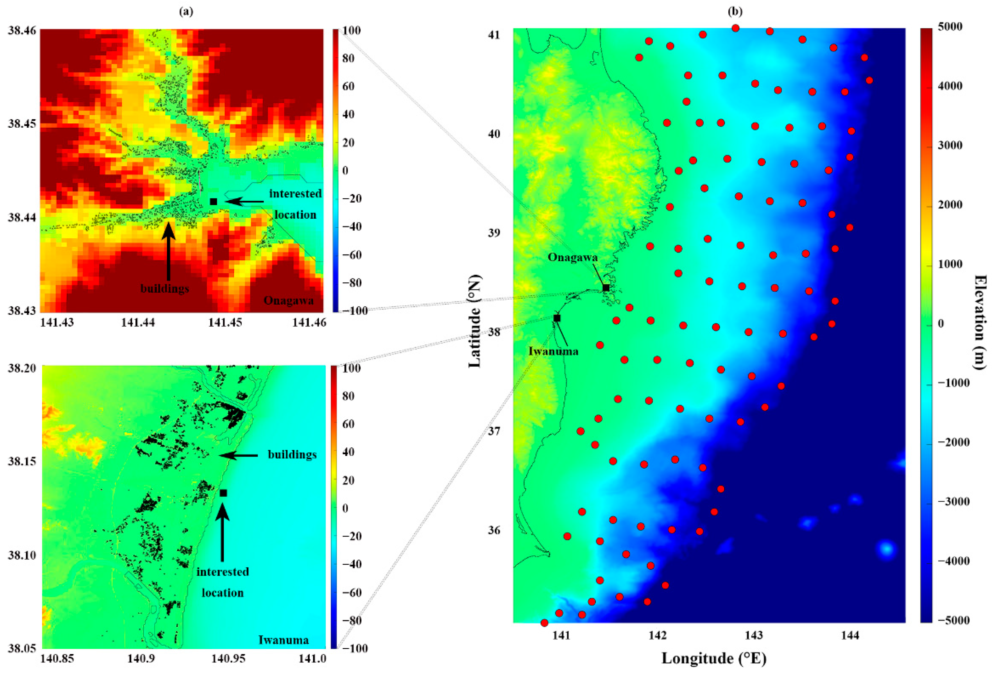
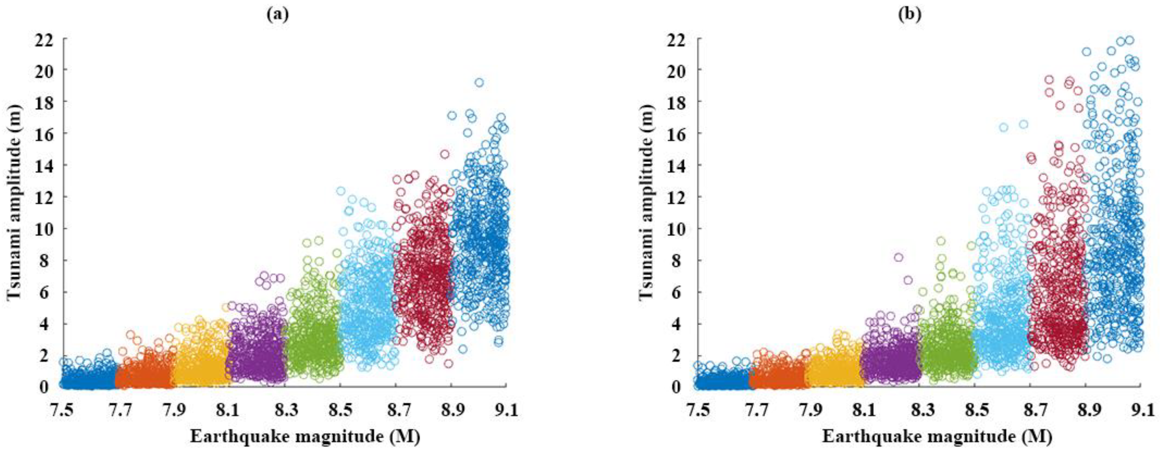
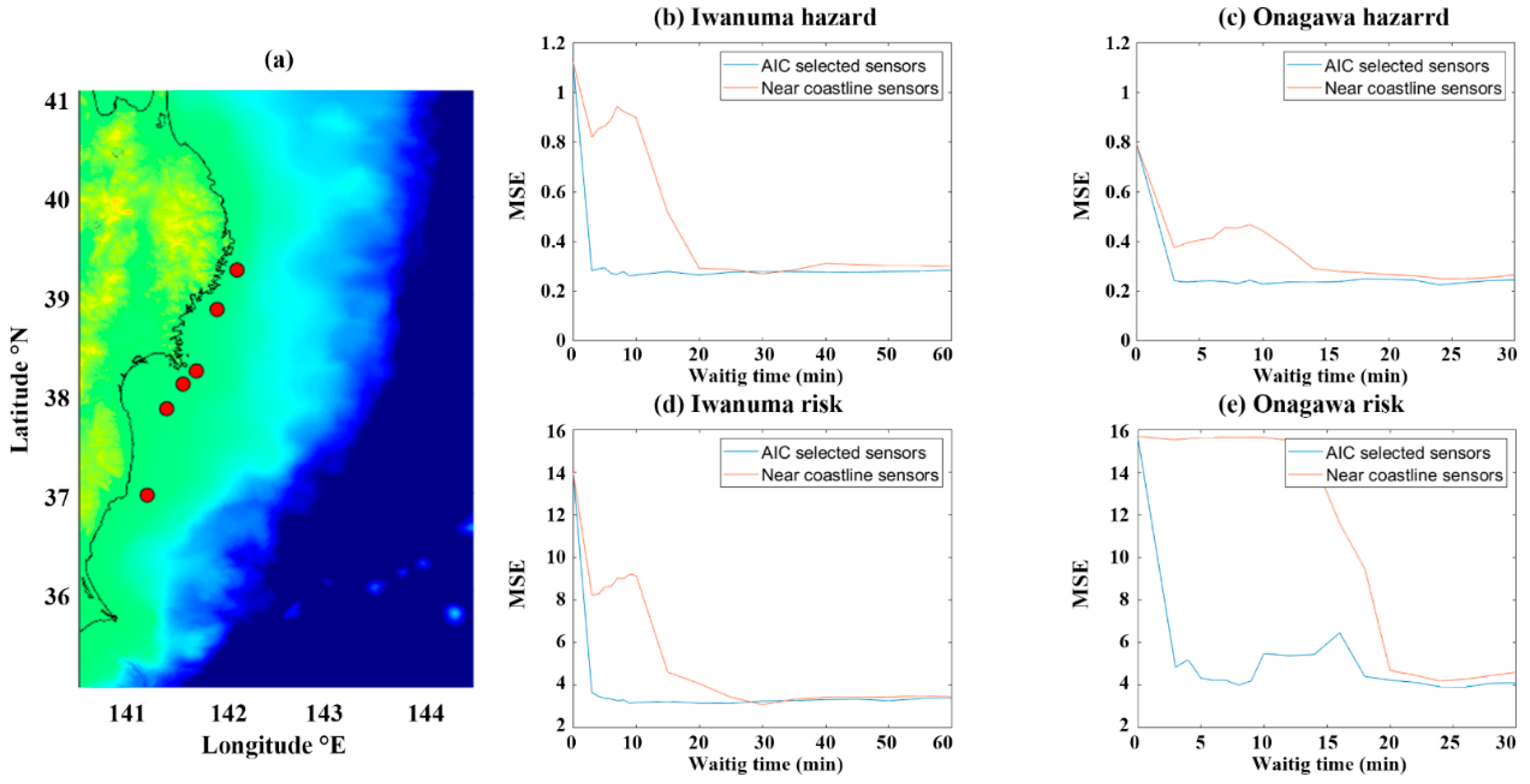
3.1.1. Maximum On-Shore Amplitude for Iwanuma

Figure 9 presents the results of the hazard-based early warning model for Iwanuma. The AIC score plot (Figure 9a) identifies an optimal configuration of recording sensors for different criteria (i.e., M3 and M4), noting that each point on the plot corresponds to a set of selected off-shore sensors. The AIC score (Figure 9a) decreases significantly from the base model to the model with the knee-point (around 5 to 10 sensors) and then decreases slowly to the model with the minimum point (around 25 to 42 sensors). The average minimum points and knee-points are 35 and 6 stations, and these correspond to $k1$ and $k2$ in Equations (5) and (6).

The MSE–waiting time plot shows a trade-off between the model performance against waiting time, and Figure 9b shows the MSE of M3 (base plus 35 sensors information) and M4 (base plus 6 sensors information). A time that achieves a stable forecasting performance is chosen as an optimal waiting time. By observing that MSE decreases significantly after 3 min and becomes relatively flat after that, the suggested waiting time is 3 min for both models.

The sensor maps for the optimal system configuration based on the AIC score plot and the MSE-waiting time plot are shown in Figure 9c,d for M3 and M4, respectively. The selected sensors for M3 cover the whole region of the S-net sensors comprehensively, whereas the selected sensors for M4 tend to include one sensor close to Iwanuma and five sensors far from the coastline and spanning from north to south. The identified configuration of the sensors for M3 attempts to utilize all available real-time wave information, while the sensor configuration for M4 attempts to cover areas near the trench where large earthquake slip asperities are located and to ensure the monitoring and detection of significant local or near-shore events by having a close-by sensor.

Figure 10 shows how the spatial locations of the selected sensors for M4 change when the waiting time changes in forecasting the maximum on-shore tsunami amplitude in Iwanuma. Figure 10a shows the selected six sensors when the waiting time is 5 min. The sensors tend to be far from the coastline. As the waiting time increases to 10 min (Figure 10b) and 20 min (Figure 10c), the selected sensors tend to be closer to the coastline, and more sensors are selected toward the direction of Iwanuma with respect to the center of the rupture area. From the MSE plot (Figure 10b), the MSE values of M3 and M4 have similar trends and are close to each other. The performance of M3 and M4 in terms of MSE is not significantly different.

Table 1. Summary of the model performances of the hazard-based and risk-based early warning systems for Iwanuma and Onagawa. The values shown in the table are MSE based on the maximum on-shore wave amplitude (hazard-based) and the tsunami loss (risk-based).

Model	MSE Based on Maximum On-Shore Amplitude		MSE Based on Tsunami Loss
	Iwanuma	Onagawa	Iwanuma	Onagawa
M1	1.12	0.79	6.45	9.60
M2	0.25	0.20	3.10	3.84
M3	0.28	0.21	3.16	3.93
M4	0.26	0.23	3.51	4.48

summarizes the mean values of the MSE with regard to forecasting the maximum on-shore tsunami amplitude in Iwanuma. M2, M3 and M4 have significantly lower MSE values compared to M1, clearly demonstrating that a small number of pre-selected S-net sensors, which measure the wave amplitude during an early period after an earthquake, provide useful information for forecasting the tsunami hazard in Iwanuma.

3.1.2. Maximum On-Shore Amplitude for Onagawa

The general observations of the results for Onagawa are similar to those for Iwanuma. The AIC score (Figure 11a) decreases significantly from the base model to the model with the knee-point (around 5 to 10 sensors). The AIC score decreases slowly to the minimum point (around 30 to 45 sensors). Figure 11b shows the MSE for M3 (base plus 35 sensors information) and M4 (base plus 6 sensors information), and the suggested waiting time is 3 min for both models (same as Section 3.1.1). Given the number of sensors added to the model and the waiting time, the selected sensors for M3 and M4 are shown in Figure 11c,d. The selected sensors for M3 cover the entire region of the S-net, whereas the selected sensors for M4 are located far from the coastline only with one sensor close to Onagawa.

Figure 12 shows how the spatial locations of the selected sensors for M4 change when the waiting time changes in forecasting the maximum on-shore tsunami amplitude in Onagawa. With the increase in waiting time, the locations of off-shore stations tend to be close to Onagawa. The summary MSE values for the Onagawa are also listed in Table 1. The consistency of the results for Iwanuma and Onagawa give greater confidence in the stability of the identified optimal configurations of the hazard-based tsunami early warning models.

3.2. Risk-Based Results

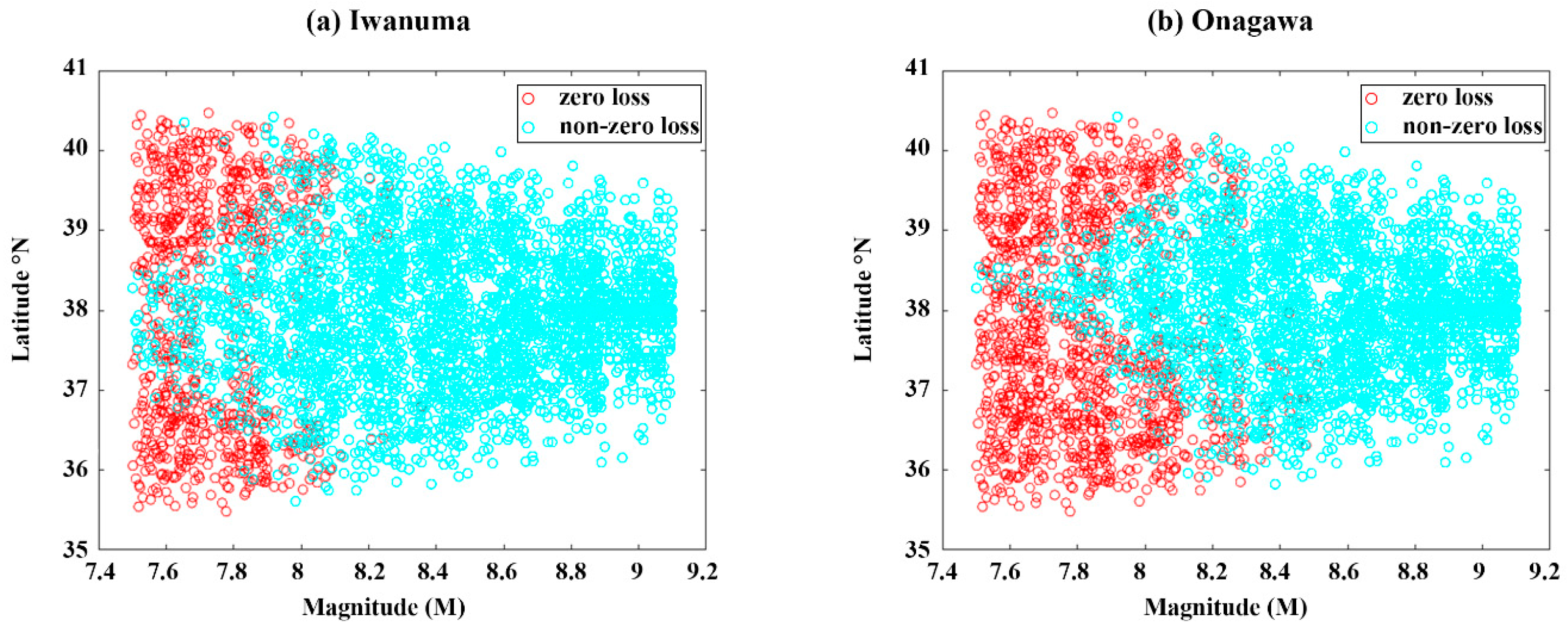
3.2.1. Tsunami Loss for Iwanuma

The AIC score (Figure 13a) decreases significantly from the base model to the model with the knee-point (around 5 to 10 sensors) and decreases slowly to the minimum point (around 20 to 42 sensors). Figure 13b shows the MSE of M3 (base plus 33 sensors information) and M4 (base plus 6 sensors information), and the suggested waiting time is 5 min for both models, similar to the optimal waiting time of 3 min using the hazard-based algorithm. Given the number of sensors added to the model and the waiting time, the selected sensors for M3 and M4 are shown in Figure 13c,d. The selected sensors for M3 cover the whole region of the S-net, whereas the selected sensors for M4 are located more evenly (one near the coastline, three in the middle, and two far from the coastline) compared to Section 3.1.

Figure 14 shows how the spatial locations of the selected sensors for M4 change when the waiting time changes in forecasting the tsunami loss in Iwanuma. Table 1 lists the mean values of the MSE with regard to forecasting the tsunami loss in Iwanuma. The smaller values of MSE for M2, M3 and M4, compared to M1, clearly suggest that S-net sensors provide useful information for forecasting the tsunami risk in Iwanuma. The performance of M3 in forecasting the tsunami amplitude in Iwanuma is better than M4 (see Figure 13b and Table 1). The result indicates that a more comprehensive coverage of the seismic rupture areas facilitates the improved forecasting of the regional tsunami consequences, which tend to be more variable and exhibit more nonlinear increasing trends compared with the maximum on-shore tsunami amplitude.

3.2.2. Tsunami Loss for Onagawa

The AIC score (Figure 15a) decreases significantly from the base model to the model with the knee-point (around 5 to 10 sensors) and decreases slowly to the minimum point (around 18 to 28 sensors). Figure 15b shows the MSE for M3 (base plus 24 sensors information) and M4 (base plus 6 sensors information), and the suggested waiting time is 10 min for both models. Given the number of sensors added to the model and the waiting time, the selected sensors for M3 and M4 are shown in Figure 15c,d. The selected sensors for M3 cover the S-net, whereas many of the selected sensors for M4 are located far from the coastline only with one close to Onagawa, and they are widely located.

Figure 16 shows how the spatial locations of the selected sensors in M4 change when the waiting time changes in forecasting the tsunami loss in Onagawa. As the waiting time increases, the locations of the off-shore stations tend to be close to Onagawa (same as the previous three analyses). The summary MSE (based on tsunami loss) values for Onagawa, summarized in Table 1, also indicate that the more spacious S-net off-shore sensors that are distributed, the higher the accuracy of the loss estimation can be. The consistency of longer waiting time in the risk-based results suggests that forecasting the tsunami loss can be an effective way to update the tsunami early warning.

4. Discussion

4.1. Challenges in Practical Applications

The results shown in Section 3 are insightful in developing early warning systems based on an extensive OBS network. For the hazard-based models, the AIC-based model (M3) suggests that a set of 25–35 sensors that span across the rupture area is needed, while the knee-point-based model (M4) indicates that a smaller set of six sensors can be enough for establishing an effective early warning system. For the hazard-based model, a short waiting time of 3–5 min is sufficient, while for the risk-based model, a longer waiting time of 5–10 min will ensure stable forecasting. These results indicate that the warning system can be designed to release multiple updates at certain times. Early-phase warning messages could be focused on maximum tsunami wave amplitude, while at later times, the warning could be updated by focusing on possible tsunami consequences. Although issuing multiple warnings can cause some confusion, these warning procedures together with how to interpret these warning messages should also be clearly communicated with evacuees, since any warning messages cannot be free from false warning messages.

The short waiting time of 3 to 5 min for the hazard-based forecasting is only achieved by the extensive spatial coverage of the S-net. A conventional wave-monitoring network tends to have stations along the coastline, lacking the coverage in the off-shore rupture area. When the monitoring sensors are relatively far from the rupture area, a short waiting time is difficult to achieve. To demonstrate this more clearly, an additional case is investigated by restricting the available S-net stations to those close to the coastline. More specifically, since the number of selected sensors based on knee-point is six, the same number of sensors near the coastline are selected, which are shown in Figure 17a. These six sensors are the closest to Iwanuma and Onagawa. With regard to the hazard-based estimation, the model that relies on six nearshore sensors cannot achieve a forecasting performance of maximum on-shore tsunami amplitude in Iwanuma comparable to the AIC-based model until the waiting time of 20 min (Figure 17b). The same trend can be seen in the forecasting of the maximum on-shore tsunami amplitude in Onagawa (Figure 17c). The main reason for the longer waiting time is that the nearshore sensors simply cannot detect any meaningful early arrivals of potentially large tsunamis until the major tsunami waves reach these sensor locations. Note that such late detection could be fatal in issuing suitable tsunami early warnings for residents to achieve safe and timely evacuations.

In terms of risk-based forecasting, the MSE of the model with AIC-selected sensors decreases significantly in the first 10 min of waiting time and then reaches a flat trend. Whereas the MSE of the model with six near-coast sensors decreases significantly after waiting 20 min. The difference of the MSE values for the two models estimating the tsunami loss is more than estimating the tsunami amplitude (Figure 17d,e). The sensors measure wave amplitude that is more relevant to the hazard aspect of the tsunami (especially when the wave is near the coastline, it is closer to the on-shore tsunami amplitude), whereas the tsunami loss has more variability, which is difficult to forecast.

In implementing the developed tsunami early warning algorithms in reality, there will be several challenges related to missing data and large noises due to malfunctioning or maintenance of OBS sensors at the time of tsunamis. To ensure robust operation of the early warning system, multiple forecasting models can be developed for a given waiting time. As shown in Section 3, there are numerous configurations of sensors that achieve similar forecasting performance. The actual decisions for issuing warning messages can be based on an ensemble of tsunami hazard and risk forecasts based on different models, which are validated to perform equally well. In this way, the operator can minimize the chance of issuing false warning messages and avoid the failure of issuing the warning messages due to missing data and large noises. These practical aspects of the tsunami early warning systems should also be investigated in the future.

4.2. Limitations and Future Improvements

There are several limitations in the study. The first limitation is that the datasets are hypothetical. There are not enough large historical events of earthquakes and tsunamis that have occurred in a region with numerous off-shore sensors. Some bias in the results may be caused by utilizing such synthetic data. Vector quantities of the maximum on-shore tsunami amplitude and tsunami loss can be forecasted, and the algorithm can be tested more comprehensively and globally in the future [41]. Regarding the statistical method, other advanced statistical methods, such as random forest and neural network [42], can be applied to forecast the tsunami impact. Moreover, multiple sources of tsunamis, such as combination of fault displacement and underwater landslide movement [43,44], can be considered in the future.

5. Conclusions

This study developed an effective algorithm for tsunami early warning considering both hazard and risk aspects using sequential MLR. Utilizing off-shore sensors can improve the accuracy of forecasting the tsunami in terms of both tsunami amplitude and tsunami loss. The algorithm should use all off-shore sensors when they are available. Using the variable selection method implemented in this study, six off-shore sensors at specific locations improve the accuracy of forecasting tsunami most significantly. During the first 3 min after an earthquake occurs, the wave amplitude measured by the off-shore sensors contains enough information to estimate the maximum on-shore tsunami amplitude and the tsunami loss in Iwanuma A longer waiting time (5 to 10 min) can improve the forecasting of tsunami loss in Onagawa.

References

1. Mori, N.; Takahashi, T. Nationwide Post Event Survey and Analysis of the 2011 Tohoku Earthquake Tsunami. Coast. Eng. J. 2012, 54, 1250001-1–1250001-27. [Google Scholar] [CrossRef]
2. Mimura, N.; Yasuhara, K.; Kawagoe, S.; Yokoki, H.; Kazama, S. Damage from the Great East Japan Earthquake and Tsunami—A Quick Report. Mitig. Adapt. Strateg. Glob. Change 2011, 16, 803–818. [Google Scholar] [CrossRef]
3. Fire and Disaster Management Agency. 2011 Off the Pacific Coast of Tohoku Earthquake (162nd report) in Japanese. 2022. Available online: https://www.fdma.go.jp/disaster/higashinihon/items/162.pdf (accessed on 1 September 2022).
4. Emergency Disaster Response Headquarters. 2011 Off the Pacific Coast of Tohoku Earthquake (Great East Japan Earthquake) in Japanese. 2011. Available online: kantei.go.jp/saigai/pdf/201104271700jisin.pdf (accessed on 1 September 2022).
5. Maeda, T.; Obara, K.; Shinohara, M.; Kanazawa, T.; Uehira, K. Successive Estimation of a Tsunami Wavefield without Earthquake Source Data: A Data Assimilation Approach toward Real-time Tsunami Forecasting. Geophys. Res. Lett. 2015, 42, 7923–7932. [Google Scholar] [CrossRef]
6. Gusman, A.R.; Sheehan, A.F.; Satake, K.; Heidarzadeh, M.; Mulia, I.E.; Maeda, T. Tsunami Data Assimilation of Cascadia Seafloor Pressure Gauge Records from the 2012 Haida Gwaii Earthquake. Geophys. Res. Lett. 2016, 8, 4189–4196. [Google Scholar] [CrossRef]
7. Dzvonkovskaya, A.; Petersen, L.; Helzel, T.; Kniephoff, M. High-frequency Ocean Radar Support for Tsunami Early Warning Systems. Geosci. Lett. 2018, 5, 29. [Google Scholar] [CrossRef]
8. Harig, S.; Immerz, A.; Weniza; Griffin, J.; Weber, B.; Babeyko, A.; Rakowsky, N.; Hartanto, D.; Nurokhim, A.; Handayani, T.; et al. The Tsunami Scenario Database of the Indonesia Tsunami Early Warning System (InaTEWS): Evolution of the Coverage and the Involved Modeling Approaches. Pure Appl. Geophys. 2019, 177, 1379–1401. [Google Scholar] [CrossRef]
9. Esposito, M.; Palma, L.; Belli, A.; Sabbatini, L.; Pierleoni, P. Recent Advances in Internet of Things Solutions for Early Warning Systems: A Review. Sensors 2022, 22, 2124. [Google Scholar] [CrossRef]
10. Hosiba, M.; Ozaki, T. Earthquake Early Warning and Tsunami Warning of JMA for the 2011 off the Pacific Coast of Tohoku Earthquake. Zisin (J. Seismol. Soc. Japan. 2nd Ser.) 2012, 64, 155–168. [Google Scholar]
11. Srinivasa Kumar, T.; Manneela, S. A Review of the Progress, Challenges and Future Trends in Tsunami Early Warning Systems. J. Geol. Soc. India 2021, 97, 1533–1544. [Google Scholar] [CrossRef]
12. Sato, M.; Ishikawa, T.; Ujihara, N.; Yoshida, S.; Fujita, M.; Mochizuki, M.; Asada, A. Displacement above the Hypocenter of the 2011 Tohoku-Oki Earthquake. Science 2011, 332, 1395. [Google Scholar] [CrossRef]
13. Kanazawa, T. Japan Trench Earthquake and Tsunami Monitoring Network of Cable-linked 150 Ocean Bottom Observatories and its Impact to Earth Disaster Science. In Proceedings of the 2013 IEEE International Underwater Technology Symposium (UT), Tokyo, Japan, 5–8 March 2013; pp. 1–5. [Google Scholar] [CrossRef]
14. Uehira, K.; Mochizuki, M.; Kanazawa, T.; Shiomi, K.; Kunugi, T.; Aoi, S.; Matsumoto, T.; Sekiguchi, S.; Yamamoto, N.; Takahashi, N.; et al. S-net project: Construction of Large-scale Seismic and Tsunami Observation System on Seafloor along the Japan Trench. In Proceedings of the 20th EGU General Assembly, EGU2018, Vienna, Austria, 4–13 April 2018; p. 12000. [Google Scholar]
15. Goda, K.; Mai, P.M.; Yasuda, T.; Mori, N. Sensitivity of Tsunami Wave Profiles and Inundation Simulations to Earthquake Slip and Fault Geometry for the 2011 Tohoku Earthquake. Earth Planets Space 2014, 66, 105. [Google Scholar] [CrossRef]
16. Goda, K.; Yasuda, T.; Mori, N.; Maruyama, T. New Scaling Relationships of Earthquake Source Parameters for Stochastic Tsunami Simulation. Coast. Eng. J. 2016, 58, 1650010–1650011. [Google Scholar] [CrossRef]
17. Mai, P.M.; Thingbaijam, K.K.S. SRCMOD: An Online Database of Finite-Fault Rupture Models. Seismol. Res. Lett. 2014, 85, 1348–1357. [Google Scholar] [CrossRef]
18. Goda, K. Multi-hazard Parametric Catastrophe Bond Trigger Design for Subduction Earthquakes and Tsunamis. Earthq. Spectra 2021, 37, 1827–1848. [Google Scholar] [CrossRef]
19. Akaike, H. Maximum Likelihood Identification of Gaussian Autoregressive Moving Average Models. Biometrika 1973, 60, 255–265. [Google Scholar] [CrossRef]
20. Thomas, C.; Sheldon, B. The Knee of a CurveUseful Clue but Incomplete Support. Mil. Oper. Res. 1999, 4, 17–24. [Google Scholar] [CrossRef]
21. Lopatka, A. Deploying Seismometers where They’re Needed Most: Underwater. Phys. Today 2019. [Google Scholar] [CrossRef]
22. Angove, M.; Arcas, D.; Bailey, R.; Carrasco, P.; Coetzee, D.; Fry, B.; Gledhill, K.; Harada, S.; von Hillebrandt-Andrade, C.; Kong, L.; et al. Ocean Observations Required to Minimize Uncertainty in Global Tsunami Forecasts, Warnings, and Emergency Response. Front. Mar. Sci. 2019, 6. [Google Scholar] [CrossRef]
23. Fraser, S.; Raby, A.; Pomonis, A.; Goda, K.; Chian, S.C.; Macabuag, J.; Offord, M.; Saito, K.; Sammonds, P. Tsunami Damage to Coastal Defences and Buildings in the March 11th 2011 M w 9.0 Great East Japan Earthquake and Tsunami. Bull. Earthq. Eng. 2012, 11, 205–239. [Google Scholar] [CrossRef]
24. Shibayama, T.; Esteban, M.; Nistor, I.; Takagi, H.; Thao, N.D.; Matsumaru, R.; Mikami, T.; Aranguiz, R.; Jayaratne, R.; Ohira, K. Classification of Tsunami and Evacuation Areas. Nat. Hazards 2013, 67, 365–386. [Google Scholar] [CrossRef]
25. Hadihardaja, I.K.; Latief, H.; Mulia, I.E. Decision Support System for Predicting Tsunami Characteristics along Coastline Areas based on Database Modelling Development. J. Hydroinformatics 2010, 13, 96–109. [Google Scholar] [CrossRef]
26. Witter, R.C.; Zhang, Y.; Wang, K.; Priest, G.R.; Goldfinger, C.; Stimely, L.L.; English, J.T.; Ferro, P.A. Simulating Tsunami Inundation at Bandon, Coos County, Oregon, Using Hypothetical Cascadia and Alaska Earthquake Scenarios. Or. Dep. Geol. Miner. Ind. Spec. Pap. 2011, 43, 57. [Google Scholar]
27. Yeh, H.; Mason, H. Sediment Response to Tsunami Loading: Mechanisms and Estimates. Géotechnique 2014, 64, 131–143. [Google Scholar] [CrossRef]
28. Wang, Y.; Heidarzadeh, M.; Satake, K.; Mulia, I.E.; Yamada, M. A Tsunami Warning System Based on Offshore Bottom Pressure Gauges and Data Assimilation for Crete Island in the Eastern Mediterranean Basin. J. Geophys. Res. Solid Earth 2020, 125. [Google Scholar] [CrossRef]
29. An, C.; Liu, H.; Ren, Z.; Yuan, Y. Prediction of Tsunami Waves by Uniform Slip Models. J. Geophys. Res. Ocean. 2018, 123, 8366–8382. [Google Scholar] [CrossRef]
30. Wang, Y.; Satake, K. Real-Time Tsunami Data Assimilation of S-Net Pressure Gauge Records during the 2016 Fukushima Earthquake. Seismol. Res. Lett. 2021, 92, 2145–2155. [Google Scholar] [CrossRef]
31. Satake, K.; Fujii, Y.; Harada, T.; Namegaya, Y. Time and Space Distribution of Coseismic Slip of the 2011 Tohoku Earthquake as Inferred from Tsunami Waveform Data. Bull. Seismol. Soc. Am. 2013, 103, 1473–1492. [Google Scholar] [CrossRef]
32. Goto, C.; Ogawa, Y.; Shuto, N.; Imamura, F. Numerical Method of Tsunami Simulation with the Leap-frog Scheme. IOC Manual UNESCO 1997, 35, 130. [Google Scholar]
33. Okada, Y. Surface Deformation due to Shear and Tensile Faults in a Half-space. Bull. Seismol. Soc. Am. 1985, 75, 1135–1154. [Google Scholar] [CrossRef]
34. Tanioka, Y.; Satake, K. Tsunami Generation by Horizontal Displacement of Ocean Bottom. Geophys. Res. Lett. 1996, 23, 861–864. [Google Scholar] [CrossRef]
35. Japan Society of Civil Engineers. Tsunami Assessment Method for Nuclear Power Plants in Japan. 2002. Available online: jsce.or.jp/committee/ceofnp/Tsunami/eng/JSCE_Tsunami_060519.pdf (accessed on 1 September 2022).
36. De Risi, R.; Goda, K.; Yasuda, T.; Mori, N. Is Flow Velocity Important in Tsunami Empirical Fragility Modeling? Earth-Sci. Rev. 2017, 166, 64–82. [Google Scholar] [CrossRef]
37. Gusiakov, V.K. Relationship of Tsunami Intensity to Source Earthquake Magnitude as Retrieved from Historical Data. Pure Appl. Geophys. 2011, 168, 2033–2041. [Google Scholar] [CrossRef]
38. Blewitt, G.; Kreemer, C.; Hammond, W.C.; Plag, H.; Stein, S.; Okal, E. Rapid Determination of Earthquake Magnitude Using GPS for Tsunami Warning Systems. Geophys. Res. Lett. 2006, 33. [Google Scholar] [CrossRef]
39. Zou, J.; Ji, C.; Yang, S.; Zhang, Y.; Zheng, J.; Li, K. A Knee-point-based Evolutionary Algorithm Using Weighted Subpopulation for Many-objective Optimization. Swarm Evol. Comput. 2019, 47, 33–43. [Google Scholar] [CrossRef]
40. Zhao, L.; Ren, Y.; Zeng, Y.; Cui, Z.; Zhang, W. A Knee point-driven Many-objective Pigeon-inspired Optimization Algorithm. Complex Intell. Syst. 2022. [Google Scholar] [CrossRef]
41. Ren, Z.; Wang, Y.; Wang, P.; Zhao, X.; Hu, G.; Li, L. Optimal Deployment of Seafloor Observation Network for Tsunami Data Assimilation in the South China Sea. Ocean Eng. 2022, 243, 110309. [Google Scholar] [CrossRef]
42. Makinoshima, F.; Oishi, Y.; Yamazaki, T.; Furumura, T.; Imamura, F. Early Forecasting of Tsunami Inundation from Tsunami and Geodetic Observation Data with Convolutional Neural Networks. Nat. Commun. 2021, 12, 2253. [Google Scholar] [CrossRef]
43. Scicchitano, G.; Gambino, S.; Scardino, G.; Barreca, G.; Gross, F.; Mastronuzzi, G.; Monaco, C. The Enigmatic 1693 AD Tsunami in the Eastern Mediterranean Sea: New Insights on the Triggering Mechanisms and Propagation Dynamics. Sci. Rep. 2022, 12, 9573. [Google Scholar] [CrossRef]
44. Watada, S.; Kusumoto, S.; Satake, K. Traveltime Delay and Initial Phase Reversal of Distant Tsunamis Coupled with the Self-Gravitating Elastic Earth. J. Geophys. Res. Solid Earth 2014, 119, 4287–4310. [Google Scholar] [CrossRef]
Figure 1. Flowchart for generating synthetic tsunami hazard and risk data.
Geosciences 12 00350 g001
Figure 2. Map of the off-shore sensors and two interested nearshore locations. (a) Zoomed maps of the two interested coastal towns, Onagawa and Iwanuma. The black squares represent the locations where the maximum on-shore wave amplitude is forecasted for the hazard-based algorithm. (b) The 99 off-shore sensors used in this study.
Geosciences 12 00350 g002
Figure 3. Earthquake rupture and tsunami wave plots for three individual cases of (a) M7.6, (b) M8.2, and (c) M9.1. The yellow triangle represents the midpoint of the earthquake rupture. There are three off-shore sensors, which are A, B and C representing near, middle, and far locations from the coastline. A greater earthquake magnitude tends to generate a larger earthquake rupture in size and higher tsunami waves.
Geosciences 12 00350 g003
Figure 4. Maximum on-shore tsunami amplitude plot for (a) Iwanuma and (b) Onagawa.
Geosciences 12 00350 g004
Figure 5. Tsunami loss plot for (a) Iwanuma and (b) Onagawa. The tsunami loss was estimated using a currency conversion rate of USD 1 = JPY 100.
Geosciences 12 00350 g005
Figure 6. Magnitude–latitude plot for (a) Iwanuma and (b) Onagawa.
Geosciences 12 00350 g006
Figure 7. An example of knee-point and minimum point plot.
Geosciences 12 00350 g007
Figure 8. Flowchart for fitting and comparing the tsunami early warning models.
Geosciences 12 00350 g008
Figure 9. Results of the hazard-based early warning model for Iwanuma: (a) AIC score plot, (b) MSE–waiting time plot, (c) optimal sensor map for M3, and (d) optimal sensor map for M4. The pink star represents the target location (Iwanuma). The red and empty circles represent the selected and unselected sensors, respectively.
Geosciences 12 00350 g009
Figure 10. Spatial maps of sensors for the hazard-based early warning in Iwanuma: (a) 5 min, (b) 10 min, and (c) 20 min. The pink star represents the target location (Iwanuma). The red and empty circles represent the selected and unselected sensors, respectively.
Geosciences 12 00350 g010
Figure 11. Results of the hazard-based early warning model for Onagawa: (a) AIC score plot, (b) MSE-waiting time plot, (c) optimal sensor map for M3, and (d) optimal sensor map for M4. The pink star represents the target location (Onagawa). The red and empty circles represent the selected and unselected sensors, respectively.
Geosciences 12 00350 g011
Figure 12. Spatial maps of sensors for the hazard-based early warning in Onagawa: (a) 5 min, (b) 10 min, and (c) 20 min. The pink star represents the target location (Onagawa). The red and empty circles represent the selected and unselected sensors, respectively.
Geosciences 12 00350 g012
Figure 13. Results of the risk-based early warning model for Iwanuma: (a) AIC score plot, (b) MSE-waiting time plot, (c) optimal sensor map for M3, and (d) optimal sensor map for M4. The pink star represents the target location (Iwanuma). The red and empty circles represent the selected and unselected sensors, respectively.
Geosciences 12 00350 g013
Figure 14. Spatial maps of sensors for the risk-based early warning in Iwanuma: (a) 5 min, (b) 10 min, and (c) 20 min. The pink star represents the target location (Iwanuma). The red and empty circles represent the selected and unselected sensors, respectively.
Geosciences 12 00350 g014
Figure 15. Results of the risk-based early warning model for Onagawa: (a) AIC score plot, (b) MSE-waiting time plot, (c) optimal sensor map for M3, and (d) optimal sensor map for M4. The pink star represents the target location (Onagawa). The red and empty circles represent the selected and unselected sensors, respectively.
Geosciences 12 00350 g015
Figure 16. Spatial maps of sensors for the risk-based early warning in Onagawa: (a) 5 min, (b) 10 min, and (c) 20 min. The pink star represents the target location (Onagawa). The red and empty circles represent the selected and unselected sensors, respectively.
Geosciences 12 00350 g016
Figure 17. Performance comparison of six near coastline sensors with selected sensors: (a) the map of the six near coastline sensors (the red circles represent the selected six near shore sensors), (b) MSE for maximum on-shore amplitude in Iwanuma, (c) MSE for maximum on-shore amplitude in Onagawa, (d) MSE for tsunami loss in Iwanuma, and (e) MSE for tsunami loss in Onagawa.
Geosciences 12 00350 g017