Review

A 20-Year Journey of Forecasting with the “Every Earthquake a Precursor According to Scale” Model

by
David A. Rhoades
*,
Sepideh J. Rastin
and
Annemarie Christophersen
GNS Science, Lower Hutt P.O. Box 30-368, New Zealand
*
Author to whom correspondence should be addressed.
Geosciences 2022, 12(9), 349; https://doi.org/10.3390/geosciences12090349
Submission received: 1 August 2022 / Revised: 9 September 2022 / Accepted: 13 September 2022 / Published: 19 September 2022
(This article belongs to the Collection Advances in Statistical Seismology)

Abstract

:
Nearly 20 years ago, the observation that major earthquakes are generally preceded by an increase in the seismicity rate on a timescale from months to decades was embedded in the “Every Earthquake a Precursor According to Scale” (EEPAS) model. EEPAS has since been successfully applied to regional real-world and synthetic earthquake catalogues to forecast future earthquake occurrence rates with time horizons up to a few decades. When combined with aftershock models, its forecasting performance is improved for short time horizons. As a result, EEPAS has been included as the medium-term component in public earthquake forecasts in New Zealand. EEPAS has been modified to advance its forecasting performance despite data limitations. One modification is to compensate for missing precursory earthquakes. Precursory earthquakes can be missing because of the time-lag between the end of a catalogue and the time at which a forecast applies or the limited lead time from the start of the catalogue to a target earthquake. An observed space-time trade-off in precursory seismicity, which affects the EEPAS scaling parameters for area and time, also can be used to improve forecasting performance. Systematic analysis of EEPAS performance on synthetic catalogues suggests that regional variations in EEPAS parameters can be explained by regional variations in the long-term earthquake rate. Integration of all these developments is needed to meet the challenge of producing a global EEPAS model.

1. Introduction

Understanding the earthquake generation process and development of earthquake forecasting models are among the main goals of statistical seismology [1,2]. Achieving these goals requires contributions from both physical and statistical modelling. In statistical seismology major laws, including the Omori-Utsu law for aftershock rate decay [3,4] and the Gutenberg-Richter magnitude frequency law [5], were originally derived empirically as statistical relations. However, it took a long time for them to be interpreted in terms of the physics of the earthquake generation process [6,7,8,9,10,11,12]. The “Every Earthquake a Precursor According to Scale” (EEPAS) model is also based on empirical statistical relations. While we have learned a lot about these relations, we still have much to learn about their physical origin. The same holds for other attempts at predicting earthquakes like that of natural time analysis of seismicity [13].
EEPAS is a space-time point process model based on an increase of minor earthquake occurrences preceding major earthquakes, the so-called “precursory scale increase” (Ψ-) phenomenon. It employs associated predictive scaling relations of the Ψ-phenomenon to forecast future earthquake rates [14,15]. Since its introduction in 2004, EEPAS has been fitted and tested on the earthquake catalogues of New Zealand, California, Japan, and Greece [16,17,18,19,20,21,22]. It was also tested by the Collaboratory for the Study of Earthquake Predictability (CSEP), an international collaboration to test earthquake forecasting models prospectively and transparently [23]. A CSEP-compatible version of EEPAS, with three-month updating, was submitted to several regional CSEP testing centres [20,21,24,25,26]. The EEPAS model generally performs better than time-invariant models of seismicity [25,26]. It is designed to forecast the largest earthquakes in a region in the medium term—a period ranging from months to decades, depending on magnitude. EEPAS is not a complete model of seismicity, because it does not consider short-term clustering. However, when combined with short-term and time-invariant forecasting models, it has proven to provide a practical method for forecasting earthquakes over a wide range of timescales [27,28,29].
EEPAS has progressively evolved both to compensate for data limitations and enhance earthquake forecasting in combination with other models. The main motivation behind all types of EEPAS revisions is to enhance the forecasting performance, i.e., the information gain. Furthermore, in recent years our understanding about additional factors affecting the information gain, other than data limitations, has developed. Consequently, we have incorporated these aspects into the EEPAS model.
In Section 2, we discuss the Ψ-phenomenon and its associated predictive scaling relations. In Section 3, we review the formulation of the EEPAS model and how it is normally fitted and tested. In Section 4, we describe combinations of EEPAS with other models and extensions to accommodate aftershocks. In Section 5, we discuss how to compensate EEPAS forecasts for missing precursory earthquakes. In Section 6, we explore two characteristics of the Ψ-phenomenon and their impact on the EEPAS model. These are (i) dependence of precursor time on the earthquake rate and (ii) a space-time trade-off of precursory seismicity. These two characteristics were originally thought to be related but are now recognized as independent. In Section 8, we move from what we know to what we do not know and outline existing challenges in forecasting with the EEPAS model.

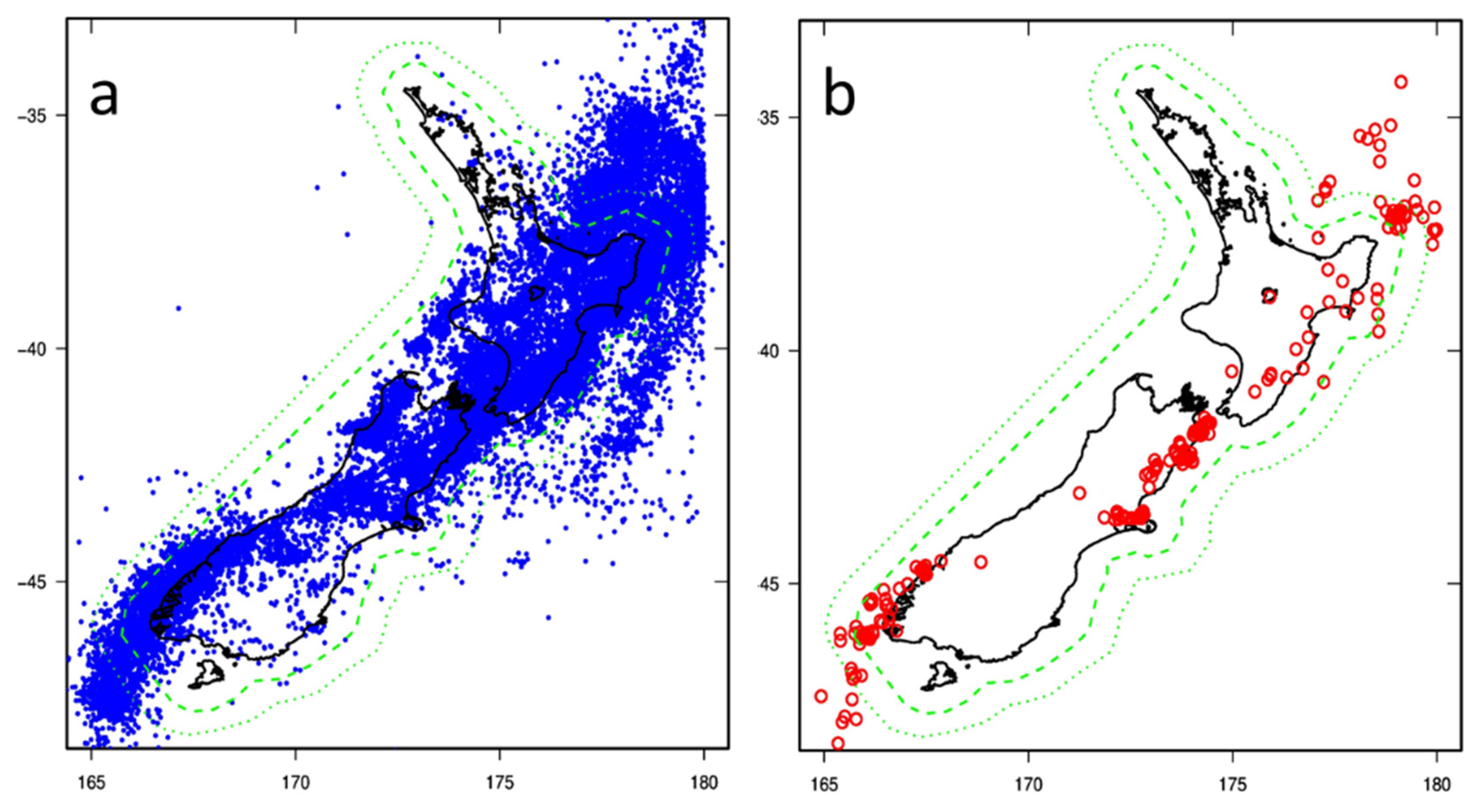
2. Empirical Foundations—The Ψ-Phenomenon

The Ψ-phenomenon is an increase in the rate and magnitude of minor earthquakes observed to occur before most major earthquakes in well-catalogued regions [14,15]. The precursor time—the time interval between the onset of the increase and major earthquake—can range from months to decades, depending on the magnitude of the major earthquake. In [15], the Ψ-phenomenon was identified for 47 major earthquakes in California and northern Mexico, Japan, Greece and northwest Turkey, and New Zealand. The onset of precursory seismicity was identified by a minimum of a cumulative magnitude anomaly (cumag) plot, in which all earthquakes in a region surrounding the major earthquake and its aftershocks over an extended time period preceding the occurrence of the major earthquake were analysed.
An identification of the Ψ-phenomenon for a recent earthquake, the M6.7 Aegean Sea event of 30 October 2020, is shown in Figure 1. In this identification, the precursors and aftershocks occurred within the rectangular area demarcated in Figure 1a. This is the precursory area, A P , of 3203 km2. The onset of precursory seismicity in 1992, following more than two decades in which no earthquakes with M ≥ 4.5 occurred, gives a precursor time, T P , of 10,220 days (Figure 1c). The average of the three largest precursory magnitudes is the precursor magnitude, M P , of 5.6 (Figure 1b).
In [15], predictive scaling relations were identified from the 47 examples of Ψ. These are of the form:
M m = a M + b M M P ;   log T P = a T + b T M P ;   and   log A P = a A + b A M P .
The first two of these relations had been known since 1977 for the precursory swarm phenomenon [30,31,32,33,34], the forerunner and a special case of the Ψ-phenomenon. Precursory swarms are an example of “precursors of the second kind”, as designated by Rikitake [35,36,37]. It shared this classification with numerous geophysical precursors for which the logarithm of precursor time was linearly related to the mainshock magnitude. The Rikitake relation was not predictive, since neither the precursor time nor the mainshock magnitude were known before the mainshock occurred. A useful feature of precursory swarms was that each swarm had an associated M P from which M m and T P of a future earthquake, or earthquakes, could be predicted (Equation (1)). It was through the learnings from extensive testing of the precursory swarm hypothesis in forecasting specific major earthquakes [38,39,40,41,42,43,44,45,46] that the more general Ψ-phenomenon was eventually recognized
The Ψ-phenomenon, unlike the precursory swarm, could not be readily identified before the occurrence of a major earthquake. Consequently, the EEPAS model was created to produce non-specific earthquake forecasts using the Ψ predictive scaling relations. EEPAS provides a generic statistical framework that regards every earthquake as a precursor of subsequent larger earthquakes. The result is a non-stationary model, which bears some similarities to the Epidemic-type-Aftershock (ETAS) model [47,48]. However, unlike ETAS, there is no suggestion that one earthquake triggers another. Instead, the magnitude of each earthquake is considered as a value of M P , i.e., a seismogenic process is assumed to be taking place on the associated scales of time, magnitude, and location indicated by (1).
The Ψ predictive scaling relations derived in [15] are plotted in Figure 2, along with data from subsequently published identifications of Ψ for major earthquakes. As well as the original 47 examples, the major earthquakes plotted include 24 further examples from Italy, New Zealand, Greece, Australia, and California [49,50,51,52,53], as well as the Aegean Sea 2020 earthquake from Figure 1. The term “major” here is used only in a relative sense, to compare an earthquake’s size with that of neighbouring events. It is obvious that the low-magnitude Australian examples of intra-plate earthquakes do not conform well to the fitted relations. This is a spur to new understandings, discussed below in Section 6.2 and Section 6.3.

3. Mathematical Description of the EEPAS Model

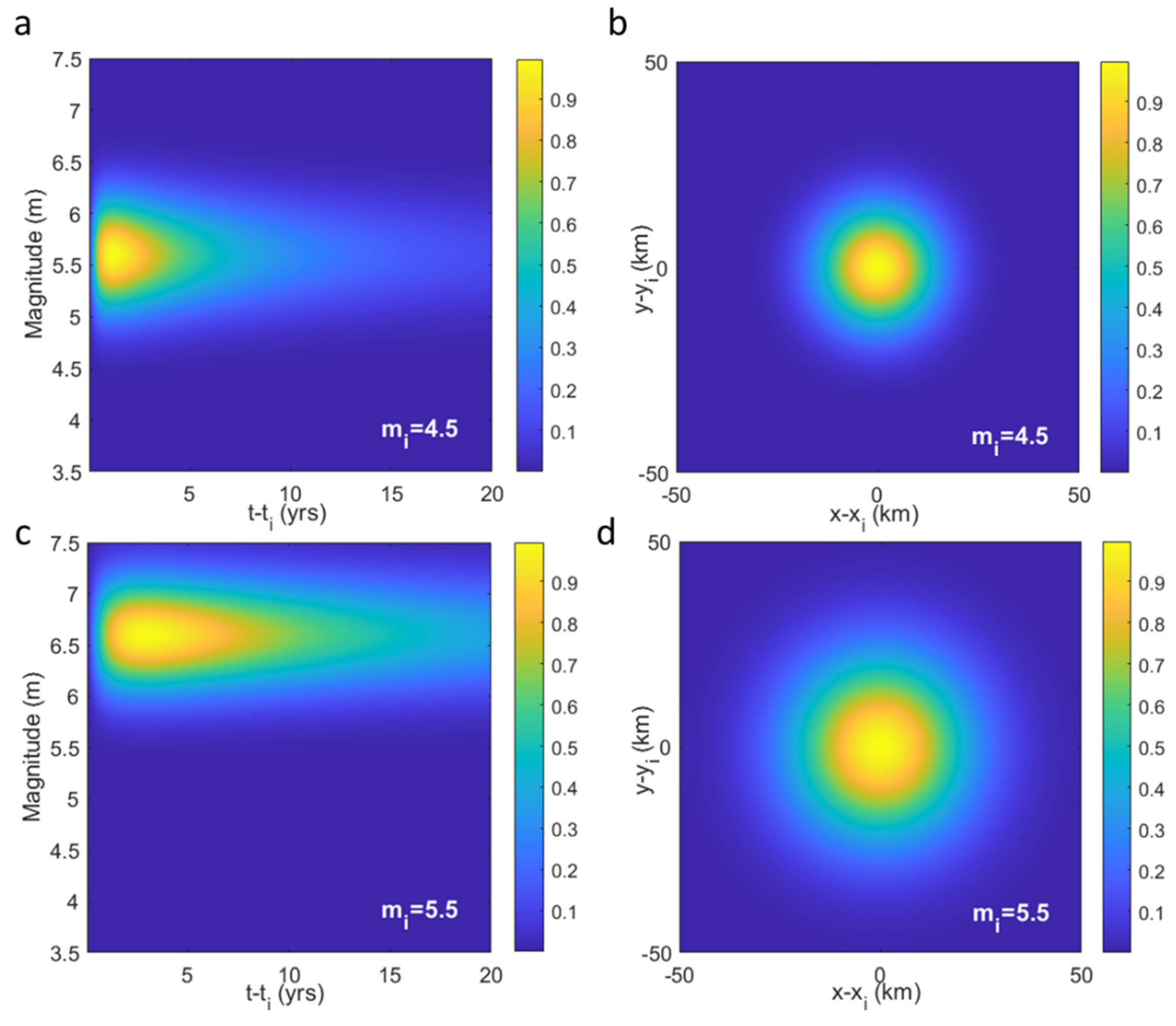
3.1. Initial Defining Equations

In the EEPAS model [16,17,18], each earthquake, with time, magnitude and location coordinates (ti,mi,xi,yi), is assumed to contribute a transient increment λi(t,m,x,y) to the future earthquake occurrence rate density in its vicinity at times t > ti, magnitudes m, and locations (x,y). The scale of its contribution is determined by its magnitude m i , taken as an instance of M P . Thus,
λ i ( t , m , x , y ) = w i f ( t | t i , m i ) g ( m | m i ) h ( x , y | x i , y i , m i ) .
Here wi is a weighting factor that can be used to emphasize earthquakes that are most likely to be precursors; f, g and h are conditional probability densities for time, magnitude and location, given mi. The magnitude density is normal and of the form
g ( m | m i ) = 1 σ M 2 π exp [ 1 2 ( m a M b M m i σ M ) 2 ]
where a M , b M , and σ M are parameters, with a M and b M based on the corresponding regression parameters in (1) and σ M on the residual standard deviation of the regression in Figure 2a. The time density is lognormal and of the form
f ( t | t i , m i ) = H ( t t i ) ( t t i ) σ T ln ( 10 ) 2 π exp [ 1 2 ( log ( t t i ) a T b T m i σ T ) 2 ]
where H(s) = 1 if s > 0 and 0 otherwise; and a T , b T , and σ T are parameters, with a T and b T based on the corresponding regression parameters in (1) and σ T on the residual standard deviation of the regression in Figure 2b. The location density is bivariate normal and of the form
h ( x , y | x i , y i , m i ) = 1 2 π σ A 2 10 b A m i exp [ ( x x i ) 2 + ( y y i ) 2 2 σ A 2 10 b A m i ]
where A and b A are parameters, with b A based on the corresponding regression parameter in (1) and log σ A 2 related to the regression parameter a A .
The probability densities in Equations (3)–(5) for precursory earthquakes with magnitudes 4.5 and 5.5 are illustrated in Figure 3.
The EEPAS model can be fitted to a catalogue with t i greater than a starting time t 0 and m i greater than a minimum magnitude threshold m 0 . The rate density λ EEPAS   ( t , m , x , y ) of earthquake occurrence within a chosen depth range is defined for time t, magnitude m > m c , and location (x,y) within a region of surveillance R. It is obtained by summing over all past occurrences, including earthquakes outside R, that could affect the rate density within R:
λ EEPAS   ( t , m , x , y ) = μ λ P P E ( t , m , x , y ) + t i t 0 , m i m 0 η ( m i ) λ i ( t , m , x , y )
where μ is a mixing parameter representing the proportion of the forecast contributed by the background model component; λ P P E is the rate density of a background Poisson model with a location distribution based on proximity to the epicenters of past earthquakes (PPE) [16,54]; t0 is the starting time of the earthquake catalogue, and η is a normalising function. For a given magnitude v, η is defined by
η ( v ) = b M ( 1 μ ) E ( w ) exp [ β ( a M + ( b M 1 ) v + σ M 2 β 2 ) ]
where E(w) is the mean weight of earthquakes in the catalogue; β = b G R   ln 10 with   b G R being the Gutenberg-Richter b-value [5]. Normalizing over the whole fitting period and region of surveillance ensures that the number of earthquakes expected by the model approximately matches the actual number of target earthquakes. It also forces the forecasted magnitudes to approximately follow the Gutenberg-Richter relation, although the magnitude distribution can vary locally from this relation. The background Poisson model also conforms to the Gutenberg-Richter relation, both locally and in the whole region R.

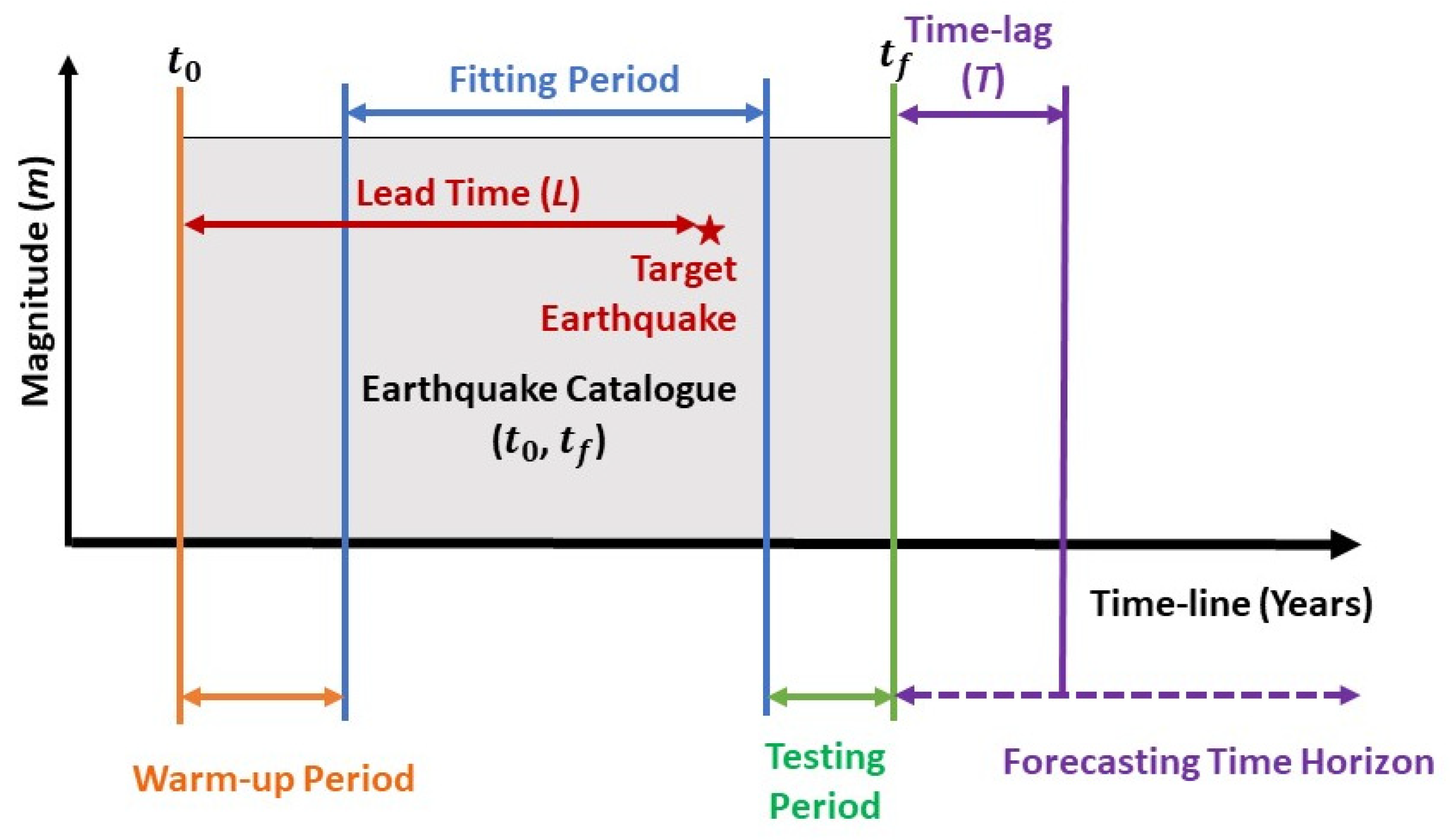
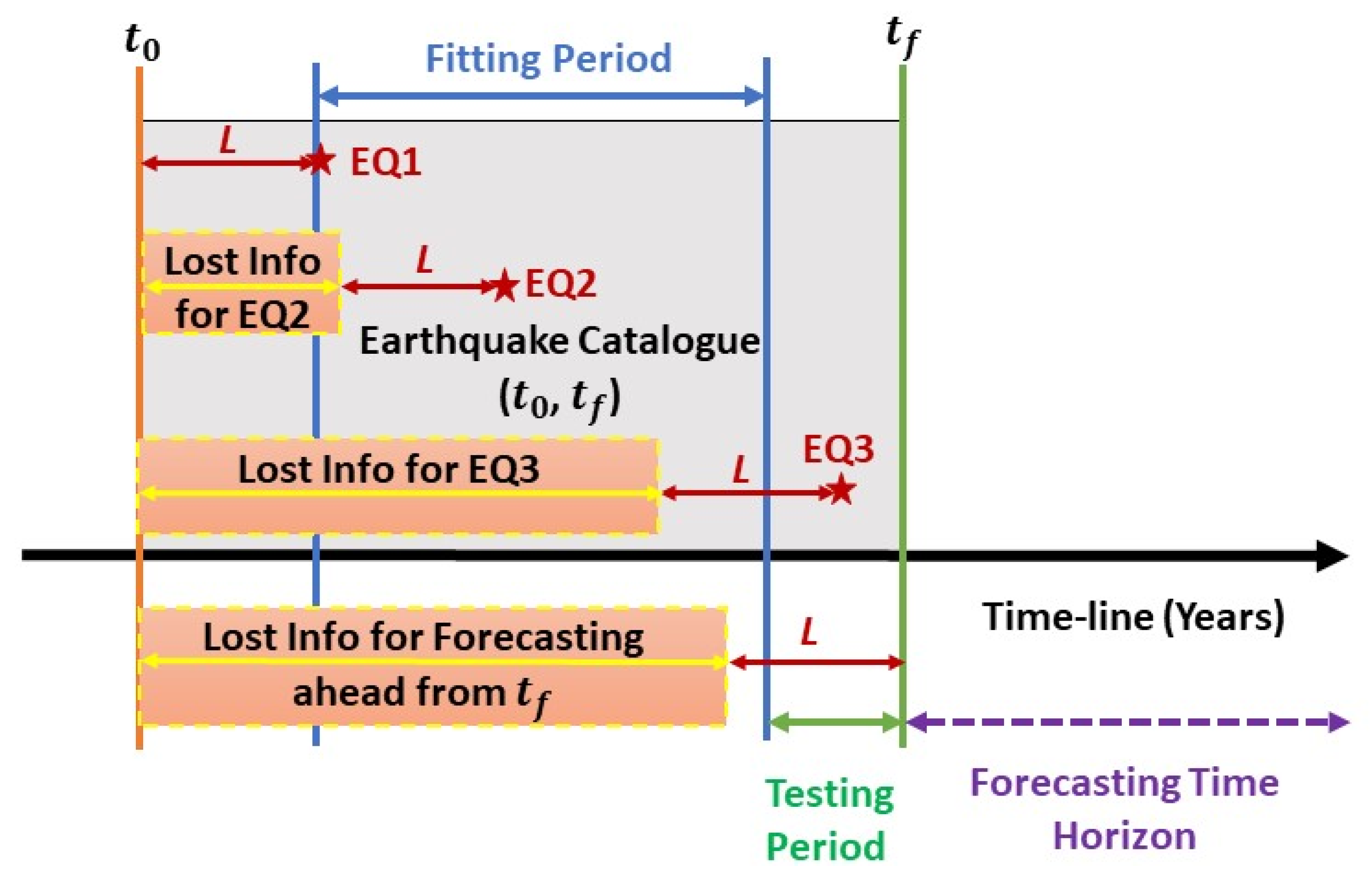
3.2. Fitting and Testing Considerations

The parameters of the EEPAS model are fitted to a chosen catalogue using the maximum likelihood method. For a model X, the log likelihood of the target earthquakes in the region of surveillance R is given [55,56] by:
ln L X = j = 1 N ln λ X ( t i j , m i j ,   x i j , y i j ) + R m c m max t a t b λ X ( t , m , x , y ) d t   d m   d x   d y
where the target earthquakes are at ( t i j , m i j ,   x i j , y i j ) ,   j = 1 ,   , N , the fitting period is ( t a , t b ), and the target magnitude range is ( m c , m max ).
EEPAS is always fitted and tested with a delay (see Table 1), which in past applications has typically been set to 50 days. This means that no earthquake is allowed to contribute to the model until 50 days after its occurrence. This delay ensures that the model will focus on timescales consistent with precursor times in examples of the Ψ-phenomenon. If no delay is applied, the parameter estimates are likely to be strongly affected by short-term clustering. Short-term clustering, such as that associated with foreshocks and aftershocks, is a much more obvious feature in earthquake catalogues than the medium-term precursory seismicity revealed by Ψ.
The original method for fitting and testing the EEPAS model is illustrated in Figure 4. The available catalogue is subdivided into three periods—a warm-up period, a fitting period, and a testing period (see Table 1 for the definitions). The purpose of the warm-up period is to provide information for fitting the model. This includes information on precursory earthquakes with magnitude M > m 0 for fitting the time-varying component and on earthquakes with magnitude M > m c for fitting the background component.
The choice of the warm-up period is crucial for the successful fitting of the model. Ideally, the warm-up period would be long enough to include all precursors to target earthquakes in the fitting period. This ideal cannot be realised in practice. Compromises must be made in subdividing the catalogue, including the choice of m0 and mc as well as the warm-up, fitting, and testing periods. Some minimum guidelines can be stated. First, the difference in m c m 0 should not be much less than 2.0, because the first Ψ scaling relation shows that the largest precursors are typically one unit of magnitude smaller than Mm and many precursors are much smaller. In some applications, m   m 0 is as low as 1.8, e.g., [16]. Secondly, the catalogue of the warm-up period should be complete for M > m c , so as not to bias the fitting of the background component. Thirdly, the catalogue should be complete for M > m 0 throughout the fitting period, and sufficiently complete in the warm-up period so that most precursors with M > m 0 to target earthquakes in the fitting period are contained in the catalogue. Here, judgements must be made. Larger target magnitudes have longer precursor times, as the Ψ scaling relations show. However, how well this guideline is met depends on the actual parameter values, which are eventually determined by fitting the model. These fitted parameters, in turn, are inevitably affected by the choices made in subdividing the catalogue.

4. Combinations and Extensions to Accommodate Aftershocks

EEPAS has been combined with a variety of independent earthquake forecasting models to improve forecasting performance in terms of the information gain statistic. The information gain per earthquake, I G , for testing pre-fitted models on an independent data set is given by
I G ( X , Y ) = ( ln L X ln L Y ) / N
where ln L X and ln L Y are the log-likelihoods of models X and Y, respectively, and N is the number of target earthquakes [59]. For a fitting period, the decrease in the corrected Akaike Information Criterion (AICc) [60,61] rather than the increase in log likelihood can be used to define IG. Model Y is typically a baseline model, e.g., the PPE background model.
Since EEPAS itself ignores aftershocks, it is to be expected that mixing it with aftershock models may improve forecasting performance. Another possibility is to extend the EEPAS model to allow for aftershocks of the major earthquakes it already forecasts. Table 2 summarizes the EEPAS major versions and corresponding references, where the reader can find details on specific applications for several regional earthquake catalogues.

4.1. STEP-EEPAS Mixture

The Short-Term Earthquake Probabilities (STEP) [66] model is an aftershock model based on the Omori–Utsu aftershock-decay relation [4]. The STEP model has a background component, λ STAT , and a time-dependent clustering component, λ CLUST . The expected number of earthquakes in the jth time, magnitude, location bin ( t j , m j ,   x j , y j ) is given by
λ STEP ( t j , m j , x j , y j ) = max [ λ CLUST ( t j , m j , x j , y j ) , λ STAT ( t j , m j , x j , y j ) ] .
STEP and EEPAS were linearly combined to enhance short-term earthquake forecasting in California [62]. Using the Advanced National Seismic System (ANSS) catalogue of California over the period 1984–2004, the optimal mixture model for forecasting earthquakes with M ≥5:0 was found to be a convex linear combination consisting of 0.42 of EEPAS and 0.58 of STEP. This mixture gave an average probability gain of more than 2 (i.e., information gain per earthquake, ln ( probability   gain ) , of more than 0.7) compared to each of the individual models when forecasting ahead for the next 24 h time period. The contribution from EEPAS can be weighted depending on magnitude to enhance the performance at high target magnitudes. The STEP-EEPAS mixture improves short-term forecasting by allowing for the aftershocks of earthquakes that have already occurred.

4.2. EEPAS with Aftershocks Model

The EEPAS with aftershocks model (EAS) [63] has a different purpose than the STEP-EEPAS mixture. It allows for aftershocks of earthquakes expected to occur under the EEPAS model, but not for aftershocks of earthquakes that have already occurred. It is aimed at improving medium-term forecasts by including the associated aftershocks of expected mainshocks in the forecast. The model assumes that the number of expected aftershocks depends on the mainshock magnitude, that their magnitude distribution follows the Gutenberg-Richter relation [67], and their spatial distribution is consistent with Utsu’s areal relation [68]. This involves a modification of the EEPAS model to include several additional parameters: the Gutenberg-Richter b-value for aftershocks, an aftershock productivity parameter θ, the minimum magnitude difference γ by which a mainshock exceeds its largest aftershock, and the proportion p M of earthquakes in the target magnitude range that are mainshocks. The effect is to change the magnitude and spatial distributions of the transient contributions of precursors to the rate density. Versions of the EEPAS and EAS model with equal weights and aftershocks down-weighted were fitted to a 10-year period and independently tested on a later 10-year period of the catalogues of California and the Kanto region of central Japan [63]. For the testing period, the information gain of the EAS models over their EEPAS counterparts was about 0.1 on average. This confirmed the efficacy of the modifications. However, the expected number of aftershocks was found to strongly depend on the assumed maximum magnitude. This creates a difficulty in the practical application of the EAS model.

4.3. Janus Model: EEPAS-ETAS Mixture

The Janus model is an additive mixture of the EEPAS model and an Epidemic-type aftershock (ETAS) model. From each contributing earthquake, it looks both to the larger earthquakes expected to follow it in the medium term and mostly smaller earthquakes expected to follow it in the short term. In [58], the Janus model was optimized for time horizons (see Table 1 for the definition) ranging from 0–3000 days (i.e., up to more than 8 years) on the New Zealand and California earthquake catalogues. For each time horizon of interest, EEPAS parameters were refitted with the delay set equal to the time horizon. It was found that the ETAS model is much more informative than EEPAS for forecasting with short-time horizons of a few days, but even with a zero-time horizon, the Janus model outperforms it with an information gain per earthquake (IGPE) of about 0.1. For time horizons of 10–3000 days, the Janus model outperforms both ETAS and EEPAS with IGPEs ranging from 0.2 to 0.5. As the time horizon lengthens beyond six months in New Zealand and two years in California, the EEPAS model becomes more informative than ETAS and the major component of the optimal mixture. In [58], it was concluded that both cascades of triggering and the precursory scale increase phenomenon contribute to earthquake predictability and that these contributions are largely independent.

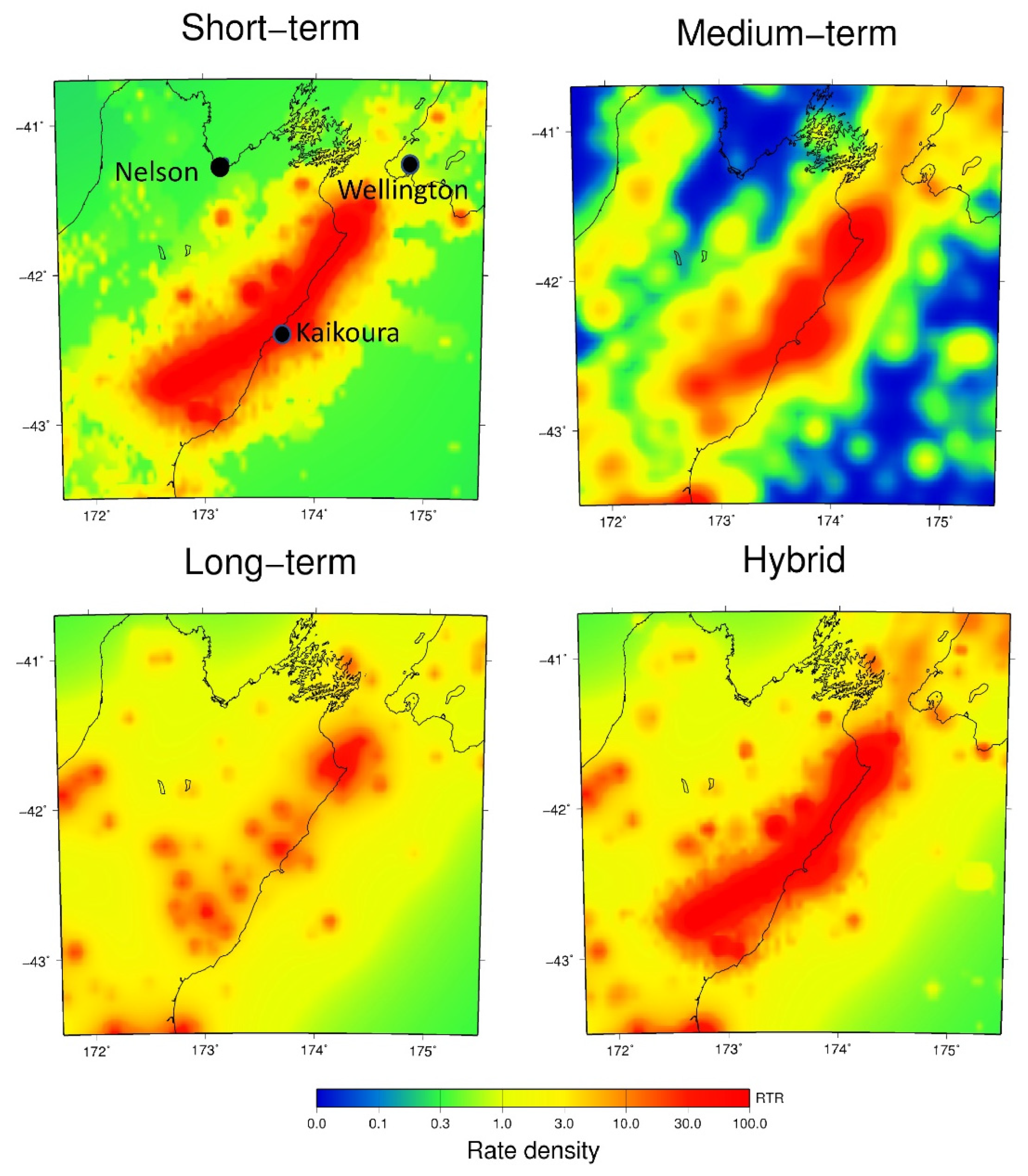
4.4. Hybrid Forecasting in New Zealand

EEPAS is now used for public earthquake forecasting in New Zealand, as one of the core elements of a hybrid forecasting tool. Public forecasting was initiated in New Zealand as a response to the devastating Canterbury earthquake sequence. This sequence began with the September 2010 M7.1 Darfield earthquake [69] and continued with the 22 February 2011 M6.3 Christchurch earthquake [70]. The Christchurch earthquake and subsequent earthquakes of about M6 in the vicinity of Christchurch resulted in the death of 185 people, and over NZ40 billion dollars of damage to buildings and infrastructure [71]. The faults that ruptured during this sequence were unknown prior to the sequence and hazard was considered to be low in Christchurch [72]. As a result of this sequence, attention was drawn to statistical forecasting models. A model with time-varying and long-term components was developed to forecast the following 50 years of expected earthquakes and resulting hazard in Canterbury. This was used to inform decisions for the rebuilding of Christchurch [28]. The time-varying component was provided by a mixture of EEPAS and aftershock models and time-invariant component by a mixture of different smoothed seismicity models [29,73]. Such statistical modelling can serve as a supplement to standard probabilistic seismic hazard analysis (PSHA) (e.g., [72,74]).
Following the November 2016 M7.8 Kaikoura earthquake [75], a modified hybrid model with three components—short-term, medium-term and long-term—was developed [27] to forecast the expected earthquakes and resulting hazard over the following 100 years. This model was used to inform decision-makers involved in the reinstatement of road and rail networks in the northern South Island. It is a gridded model, in which EEPAS provides the medium-term component. Figure 5 illustrates how the hybrid model is constructed from its three components.

5. Compensation for Incompleteness of Precursory Earthquakes

5.1. Magnitude Completeness of Precursory Earthquake Contributions

Completeness of an earthquake catalogue is usually expressed in terms of a threshold magnitude, M C . The threshold magnitude varies from one seismic network to another and also with time. For a specific M C that is valid for a period of time, all the earthquakes with magnitudes m M C are expected to be recorded in the catalogue produced by the seismic network. The value of M C depends on the signal-to-noise ratio (SNR) of the recorded waveforms and the density of the seismic network. The SNR varies based on the earthquake magnitude, epicentral distances, azimuth, fault orientation, rheology, ambient noise levels, path, and site effects [76,77,78].
The EEPAS model has a magnitude lower limit of m 0 , which is chosen so that m 0 M C during the fitting and testing period. In addition, EEPAS has a compensatory term for the precursory earthquakes with m < m 0 . Because of the missing contribution from earthquakes below magnitude m 0 , the rate density at magnitude m will be diminished, on average, to a fraction Δ ( m ) of its actual value, given by
Δ ( m ) = Φ ( m a M b M m 0 σ M 2 β σ M )
where Φ is the standard normal integral, i.e., Φ ( x ) = x exp ( u 2 2 ) d u / 2 π . To compensate for this deficiency, the estimated rate density λ ( t , m , x , y ) is inflated by a factor of 1 / Δ ( m ) [16].

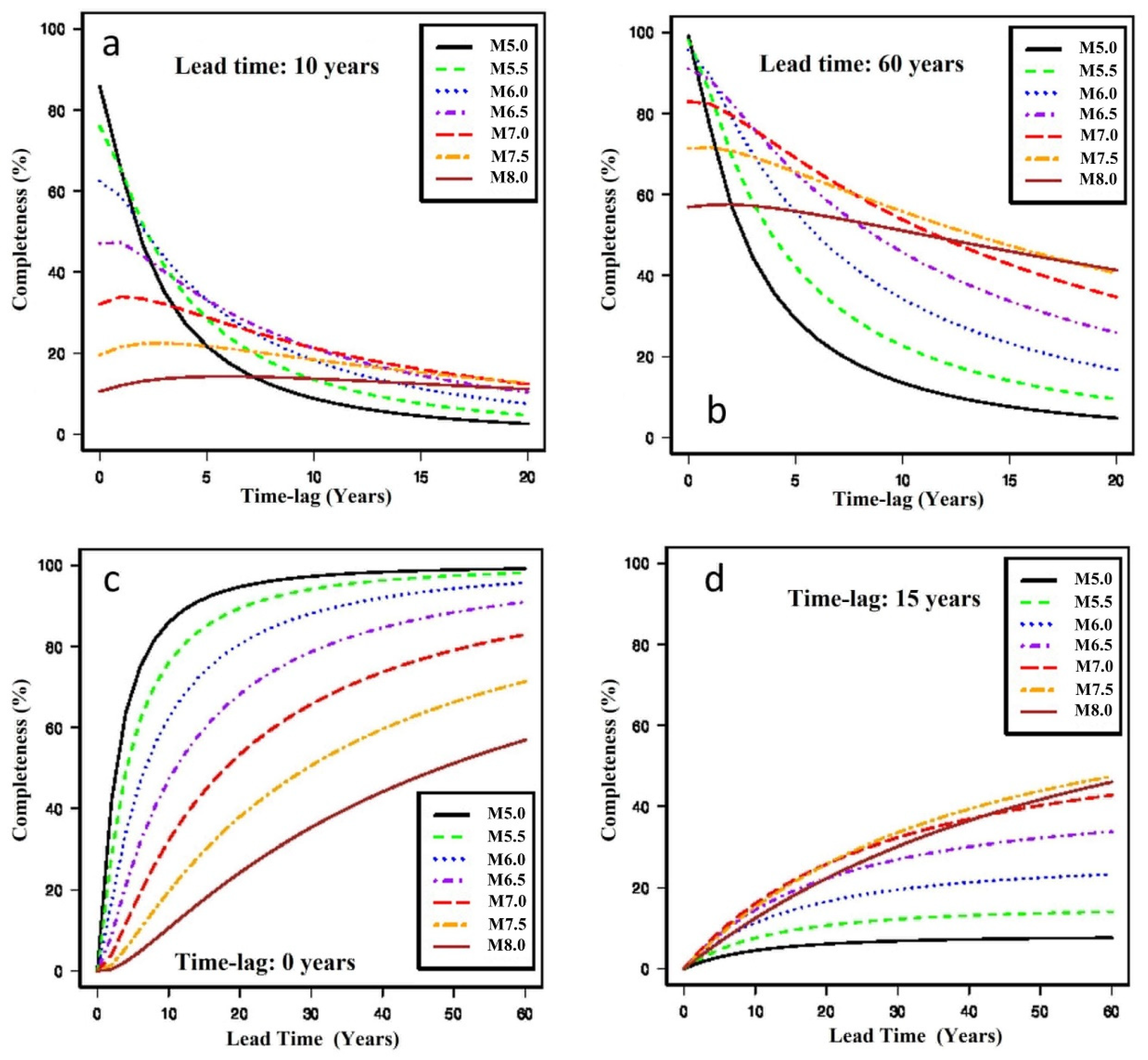
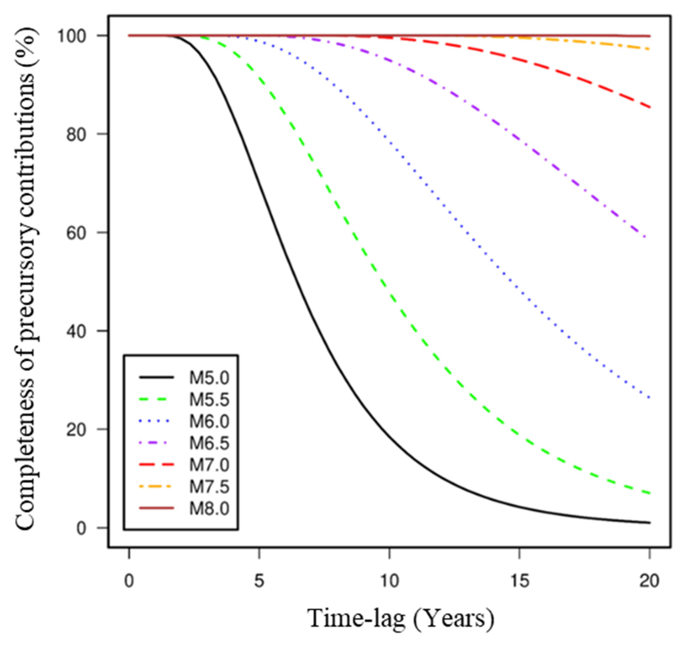
5.2. Temporal Completeness of Precursory Earthquake Contributions

A milestone in the development of EEPAS has been to compensate the forecasts for the incompleteness of precursory information before any target earthquake. This includes compensation for missing precursory earthquakes in the time-lag between the end of the catalogue and the forecasting time horizon. It also includes compensation for missing precursors before the lead time for any target earthquake. So far, we have compensated either for the time-lag or the lead time, but not simultaneously. A further milestone would be to integrate these two compensations.
Compensation for the time-lag enables the forecasting horizon to be extended from a few months to a decade or more without much loss of forecasting quality (information gain). In public forecasting, EEPAS has sometimes been applied with long time horizons (time-lags), e.g., up to 50 years in the Canterbury hybrid forecasting model [73] and up to 100 years in the Kaikoura hybrid model [27]. In the latter two models, the expected number of earthquakes forecast by the EEPAS time-varying component diminishes as the time horizon is increased. This is because no compensation is made for the missing contributions from future earthquakes between the end of the available catalogue and the future time horizon for which a forecast is being made.
In compensating for temporal incompleteness, the prior assumption is made that unknown precursory earthquakes are equally likely to occur at any time and have a magnitude distribution that conforms to the Gutenberg–Richter relation. The total contribution c ( T , L , m ) of precursory earthquakes to the rate density for a target earthquake with magnitude m as a function of the time-lag T and lead time L was given by [57] as:
c ( T , L , m ) = m 0 m u [ T T + L f ( t | t τ , v ) d τ ] η ( ν ) g ( m | v ) 10 b G R v d v .
It follows from the lognormal form of the time distribution (4) that
c ( T , L , m ) = m 0 m u [ Φ ( log ( T + L ) a T b T ν σ T ) Φ ( log T a T b T ν σ T ) ] η ( ν ) g ( m | ν ) 10 b ν d ν ,
where the logarithm is to base 10 and b is the Gutenberg-Richter b-value. The completeness of precursory earthquake contributions to a target earthquake with magnitude m when the time-lag is T and the lead time is L is then given by
p ( T , L , m ) = c ( T , L , m ) c ( 0 , , m ) ,
in which c ( 0 , , m ) = m 0 m u η ( v ) g ( m | ν ) 10 b ν d ν .
Figure 6 illustrates the completeness function, p ( T , L , m ) , for the EEPAS_0F model fitted to the New Zealand GeoNet catalogue from 1987 to 2006 [58]. The EEPAS_0F model gives equal weights to all input earthquakes. The parameters are given in Table 3.
In Figure 6, one can see that when the lead time is long and the time-lag is short, the completeness is high for all magnitudes. However, the completeness at low magnitudes is highly sensitive to an increase in time-lag T, but not so sensitive to a decrease in lead time L. The completeness at high magnitudes is more sensitive to a decrease in lead time L and less sensitive to an increase in time-lag T.
Given a set of EEPAS parameters, the corresponding completeness function and fixed values of T and L, the EEPAS model can be compensated by optimally combining two end-members, A and B. End-member A is compensated by scaling up the background component, and end-member B by scaling up the time-varying component, by the inverse of the completeness at each T, L and m. End-member A has rate density λ A ( t , m , x , y ) , given by
λ A ( t , m , x , y ) = [ μ + ( 1 μ ) ( 1 p ( T , L , m ) ) ] λ 0 ( t , m , x , y ) + t i t 0 , m i m 0 η ( m i ) λ i ( t , m , x , y ) .
End-member B has rate density λ B ( t , m , x , y ) , given by
λ B ( t , m , x , y ) = μ λ 0 ( t , m , x , y ) + 1 p ( T , L , m ) t i t 0 , m i m 0 η ( m i ) λ i ( t , m , x , y ) .
The optimal combination can be found by optimizing the parameter ω in a convex linear combination with rate density λ C ( t , m , x , y ) , given by
λ C ( t , m , x , y ) = ω λ A ( t , m , x , y ) + ( 1 ω ) λ B ( t , m , x , y ) ,
where 0 ≤ ω ≤ 1.

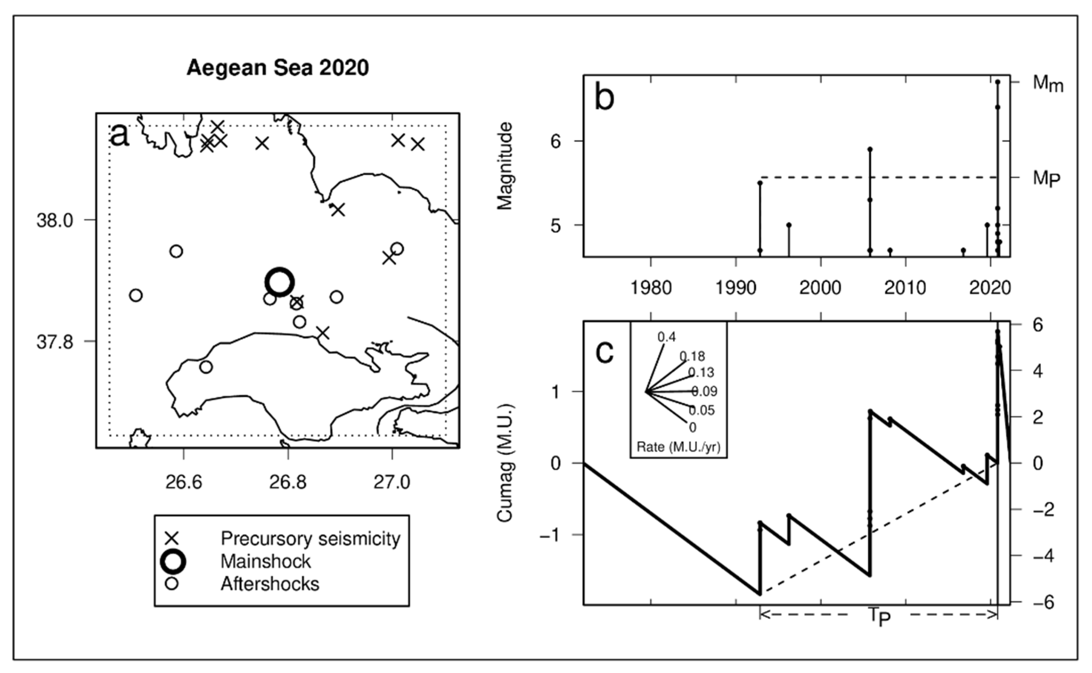
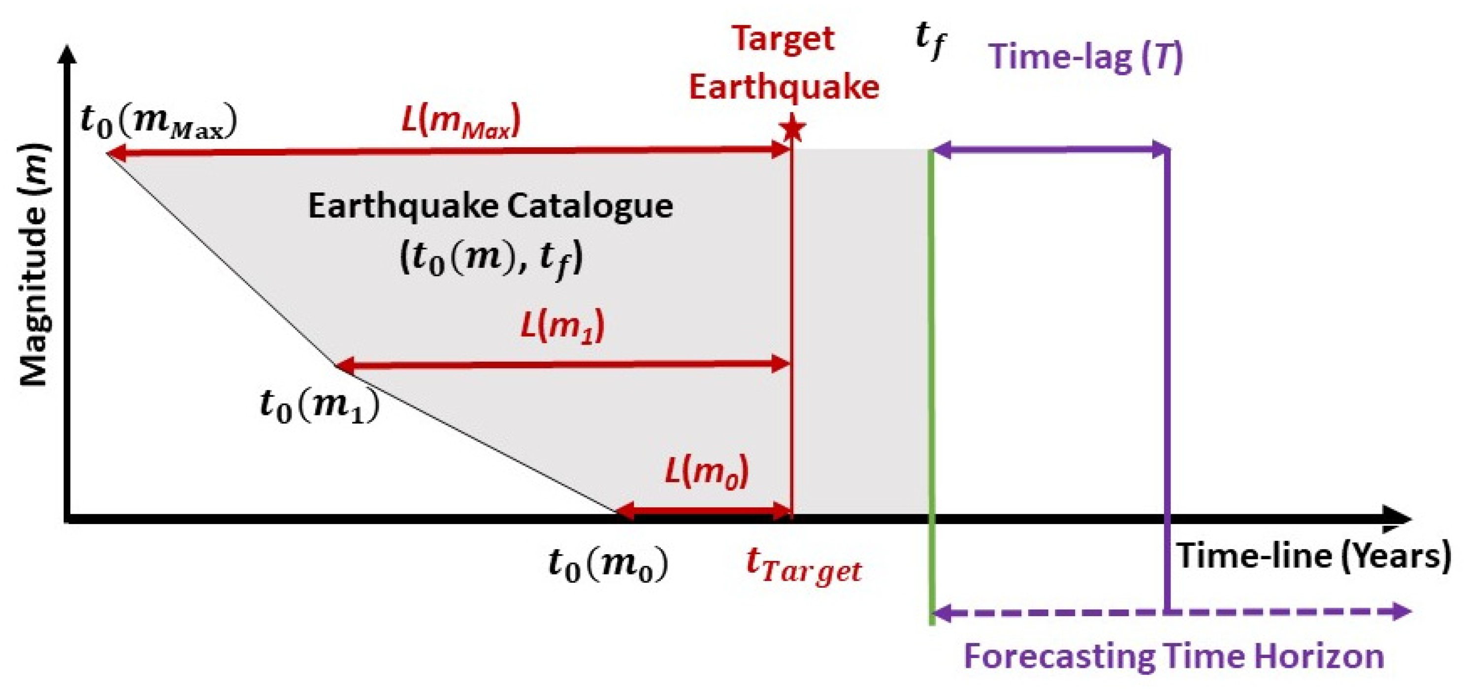
5.3. Compensation for Time-Lag

In [57], a special case of the above method was applied to compensate for incompleteness due to the time-lag (the LEEPAS model), assuming there was no significant incompleteness due to the lead time, i.e., with p ( T , L , m ) replaced by p ( T , , m ) in (15) and (16). Three versions of EEPAS applied to the New Zealand GeoNet catalogue, with different magnitude thresholds and weighting strategies, were considered. The mixing parameter ω was optimised for a range of time-lags up to 15 years. The fitted ω values were used to produce annual lag-compensated forecasts in central New Zealand out to 2030.
The method of [57] has been further applied to estimate the distributed seismicity model for the 2022 revision of the New Zealand National Seismic Hazard model (NZSHM) [79]. The NZSHM uses a version of the New Zealand earthquake catalogue obtained by adjusting the GeoNet-preferred magnitudes to be consistent with the moment magnitude [80]. We call this the Adjusted Magnitude (AMC) catalogue.
We have fitted EEPAS to the AMC catalogue with m0 = 2.95, mc = 4.95, t0 = 1951.01.01, tf = 2020.12.31, a warm-up period of 1951-2005 and a fitting period of 2006-2020, within the New Zealand CSEP testing region (Figure 7). The maximum likelihood parameters were estimated for the EEPAS_1F model (Table 4). Unlike EEPAS_0F, the EEPAS_1F model down-weights aftershocks as described in [16].
For the EEPAS_1F model, the completeness function is plotted in Figure 8. The parameter ω (Equation (17)) was fitted for time-lags up to 20 years. For each time-lag, ω is close to zero (Figure 9). This confirms that the optimal forecast is obtained by mostly compensating the time-varying component.
Despite rapidly decreasing completeness for the target earthquakes with M < 6 for time-lags greater than 10 years, the information gain of LEEPAS_1F over PPE changes only gradually with increasing time-lag (Figure 10). For example, with a time-lag of 15 years, the completeness is about 5% for M 5 (Figure 8). However, Figure 10 shows that at the same time-lag, IG(LEEPAS_1F, PPE) is 0.5. This is greater than the IG at a time-lag of 1 year.

5.4. Fixing the Lead Time

The length of the warm-up period determines the minimum lead time L for earthquakes in the fitting period. The lead time is different for every target earthquake in the fitting period, testing period, or a later period of forecasting. The fitting of parameters of the time distribution f ( t | t i , m i ) is affected by the available lead time for target earthquakes in the fitting period. The fitted time distribution is biased because of missing contributions from precursors that occurred before the start of the catalogue. In particular, shorter lead times favour smaller values of the time-scaling parameter a T . If the same catalogue start time t0 is used, target earthquakes in the testing period have longer lead times than those in the fitting period, and possibly a larger optimal value of a T . Target earthquakes in a future period of forecasting have even longer lead times.
Obviously, EEPAS forecasts are affected by not having equal lead times. To reverse this effect, the Fixed Lead time EEPAS model (FLEEPAS) was proposed [52]. In FLEEPAS, the lead time L is kept constant by restricting the precursory earthquakes contributing to the time-varying component. At a given time t, only earthquakes with t i > t L are allowed to contribute, as illustrated in Figure 11. Thus Equation (6) is replaced by
λ ( t , m , x , y ) = μ λ 0 ( t , m , x , y ) + t i t L , m i m 0 η ( m i ) λ i ( t , m , x , y )
In [52], FLEEPAS was fitted to the New Zealand GeoNet catalogue from 1987 to 2006 with a range of L values from 3 to 35 years. The parameters fitted for each value of L were a T , σ A , and μ. It was found that the value of a T increased as L was increased. This confirmed the dependence of the fitted time distribution on the lead time.
A fitted FLEEPAS model can be applied with the same lead time to a subsequent period of the catalogue, for the purpose of testing or forecasting. Then the performance is likely to match that of the fitting period, because the parameters have been optimised to the lead time. However, a disadvantage of the FLEEPAS model is that it disregards a substantial portion of the catalogue, as illustrated in Figure 11. The catalogue used by FLEEPAS may be severely lacking information on precursory earthquakes, especially for high magnitude target earthquakes.

5.5. Compensating for the Lead Time

In [52], a special case of Equations (13) and (14) was used, with the incompleteness due to the time-lag assumed to be negligible. Therefore, p ( T , L , m ) was replaced by p ( 0 , L , m ) and ω was optimised. This is the Fixed Lead Time Compensated EEPAS model (FLCEEPAS). In FLCEEPAS, ω was fitted for L values from 3 to 35 years for EEPAS_0F with other parameters as in Table 3. As shown in Figure 6c, the incompleteness was problematic for short lead times. This was addressed by FLCEEPAS, which outperformed the original EEPAS_0F model. The compensation redresses the underprediction due to incompleteness, especially at the highest target magnitudes which have lowest completeness for a given L (Figure 6c).

6. Earthquake-Rate Dependence and the Space-Time Trade-Off

6.1. An Earthquake-Rate Dependent Version of EEPAS

The Earthquake-rate dependent EEPAS model (ERDEEP) [64] was an attempt to explain the relatively low correlation between logTP and logAP compared with other correlations among M m , M P , log T P , and log A P [15,81]. The hypothesis was that the average level of seismicity in a region affects both the precursor time and precursory area in such a way that there is an even trade-off between these two. The fitted parameters of the EEPAS distributions for time and area were observed to vary significantly between regions, such as Japan and California. For example, the average level of seismicity in central Japan is about six times higher than in California. Also, the fitted values of aT and σA showed that the scale of f(t|mi) is about six times shorter and that of g(x,y|xi,yi,mi) about six times larger in central Japan than in California [82]. In the ERDEEP model, the estimated long-term seismicity rate in the jth cell of a gridded smoothed seismicity model is denoted by ρ(j). The parameters a T and σ A are both made dependent on ρ(j). The values of a T and σ A in the jth cell are defined by
a T ( j ) = a T c ρ log ρ ( j )
σ A ( j ) = σ A ρ ( j ) c ρ 2
With this definition, the product of the area-scaling factor σ A 2 ( j ) and time-scaling factor 10 a T ( j ) is held constant:
σ A 2 ( j ) 10 a T ( j ) = σ A 2 10 a T
The fitting of ERDEEP thus required the optimisation of one additional parameter c ρ along with the other EEPAS parameters. In formal CSEP testing in the New Zealand region, ρ(j) was obtained using PPE [16,54] as in the smoothed seismicity model. ERDEEP did not perform quite as well as standard EEPAS [26]. Therefore, the hypothesis on which ERDEEP is based is not supported by testing. Subsequent work has clarified the misconception underlying this hypothesis. The dependence of a T on the seismicity rate (Equation (19)) has been shown to be well-founded, as has the space-time trade-off (implied by Equation (21)). However, no evidence shows that the seismicity rate is linked to the space-time trade-off.

6.2. Rate Dependence of Time-Distribution in Synthetic Catalogues

The application of EEPAS to synthetic catalogues generated by physics-based earthquake simulators has been helpful in clarifying the dependence of a T on the earthquake rate. The EEPAS model has been applied to synthetic catalogues generated by the earthquake simulators known as ARTS [83,84] and RSQsim [85]. An advantage of synthetic catalogues is that they can span arbitrarily long time periods without any temporal variation of catalogue quality. A disadvantage is that they tend to cover a much narrower range of magnitudes than real catalogues. In [82], an ARTS synthetic catalogue based on the faults of the Wellington region, central New Zealand, was studied. In a generic fault network with one major fault and numerous parallel minor faults, the performance of the EEPAS model was found to be poor. But in a complex network of major faults at a variety of orientations and many randomly oriented small faults, EEPAS performed better. In fact, the performance was similar to that in real catalogues, albeit with some differences in the scaling of time and area. Also, the precursory scale increase phenomenon could be readily identified before most of the major synthetic earthquakes. The fault geometry therefore affects how well EEPAS fits.
In [51], RSQsim synthetic catalogues based on the same region and faults were used. Taking advantage of the ability of RSQsim to rapidly generate synthetic catalogues [85], the slip rates on all faults were systematically reduced by five successive factors of 4. Fitting the EEPAS model to these synthetic catalogues showed that the expected precursor time is inversely proportional to the reduction in slip rate. This is consistent with c ρ = 1 in Equation (19), with the logarithm being to base 10. This result suggests that the expected precursor times for large earthquakes in stable continental regions with very slow fault slip rates would go well beyond the length of available catalogues. The Australian earthquakes in Figure 2 are from a stable continental region. It is not surprising therefore to see that the T P values for Australian earthquakes are relatively large for a given M P compared with the regression computed from more seismically active regions (Figure 2b).

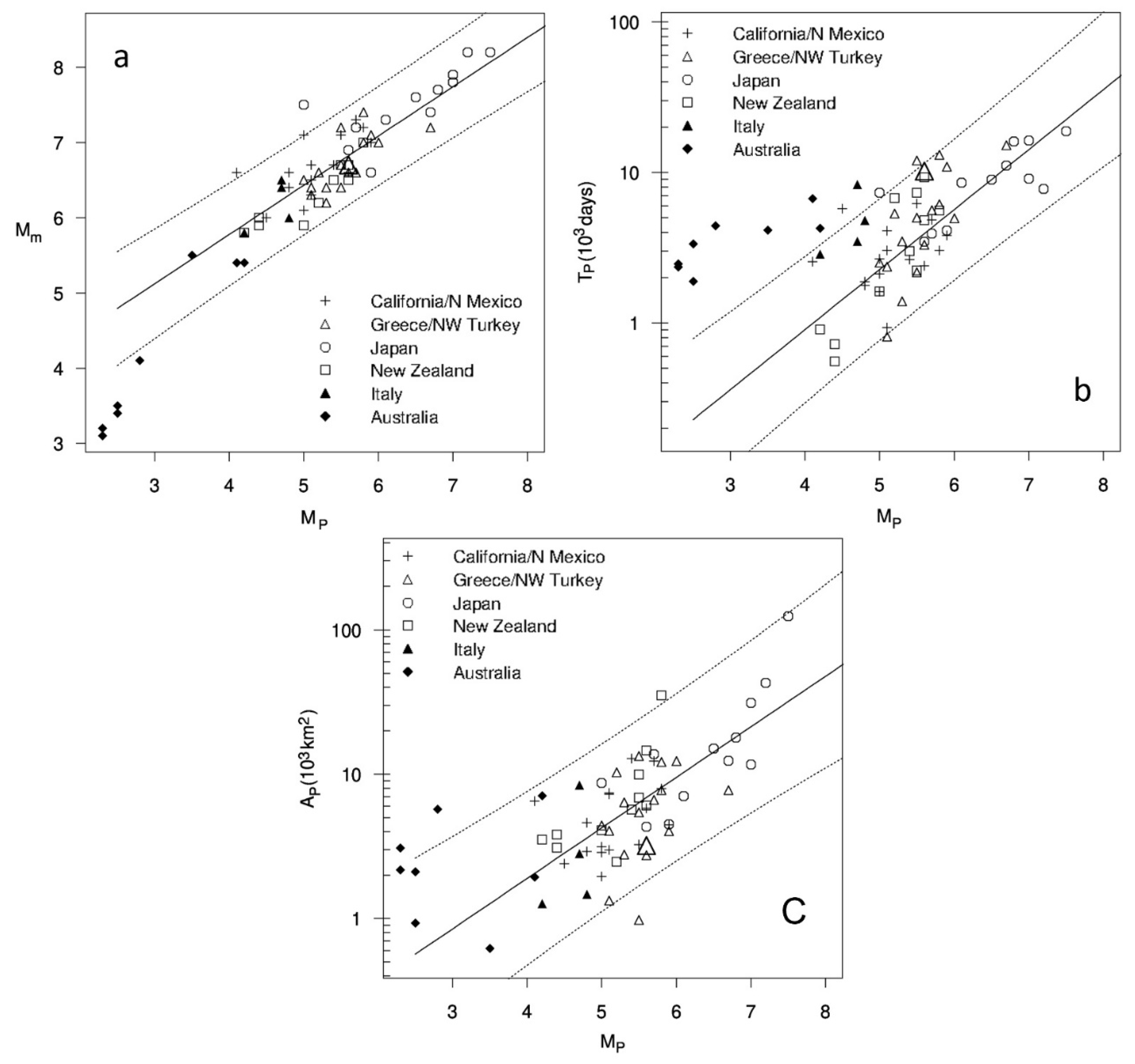
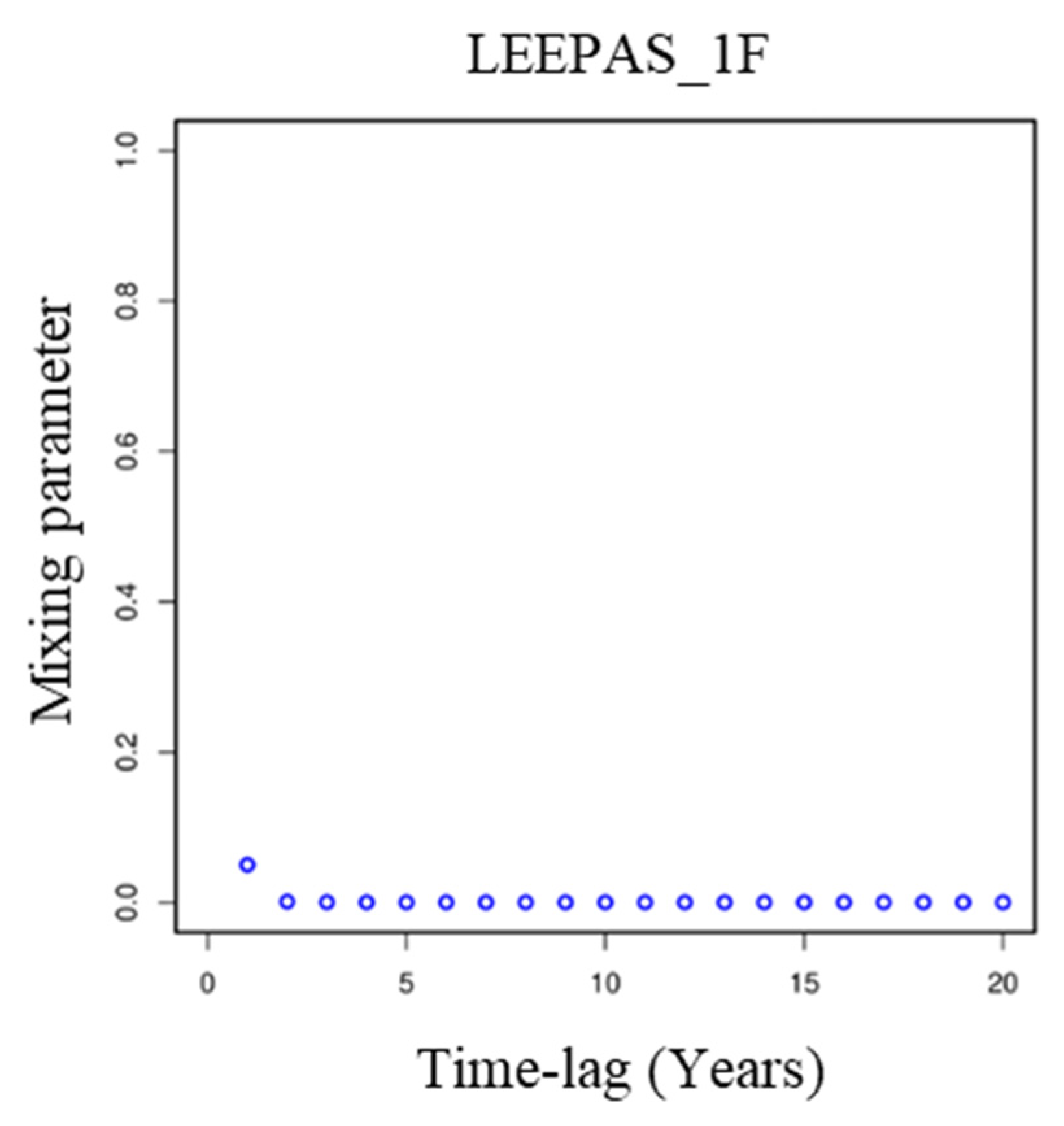
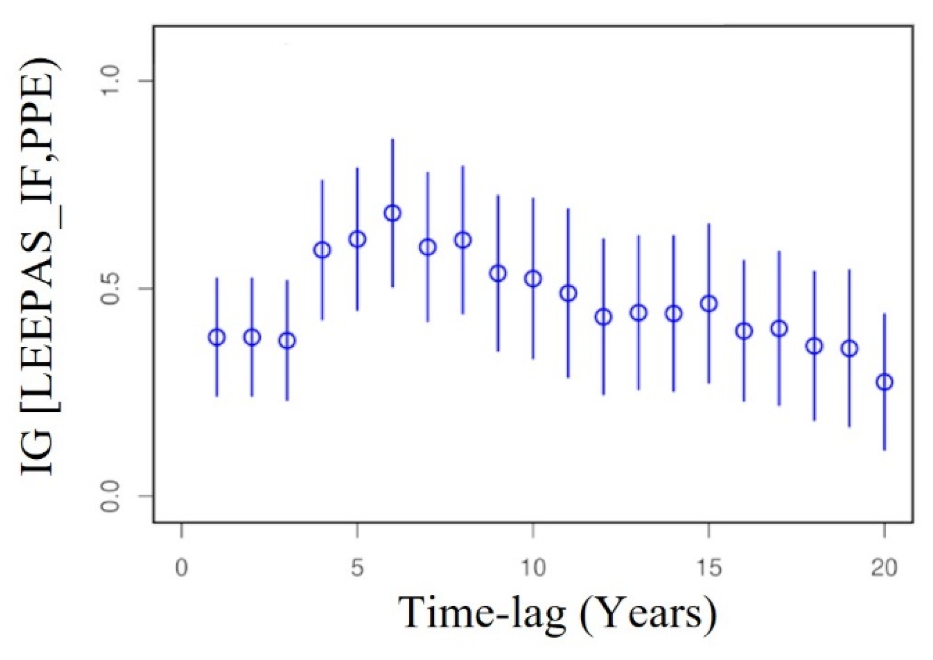
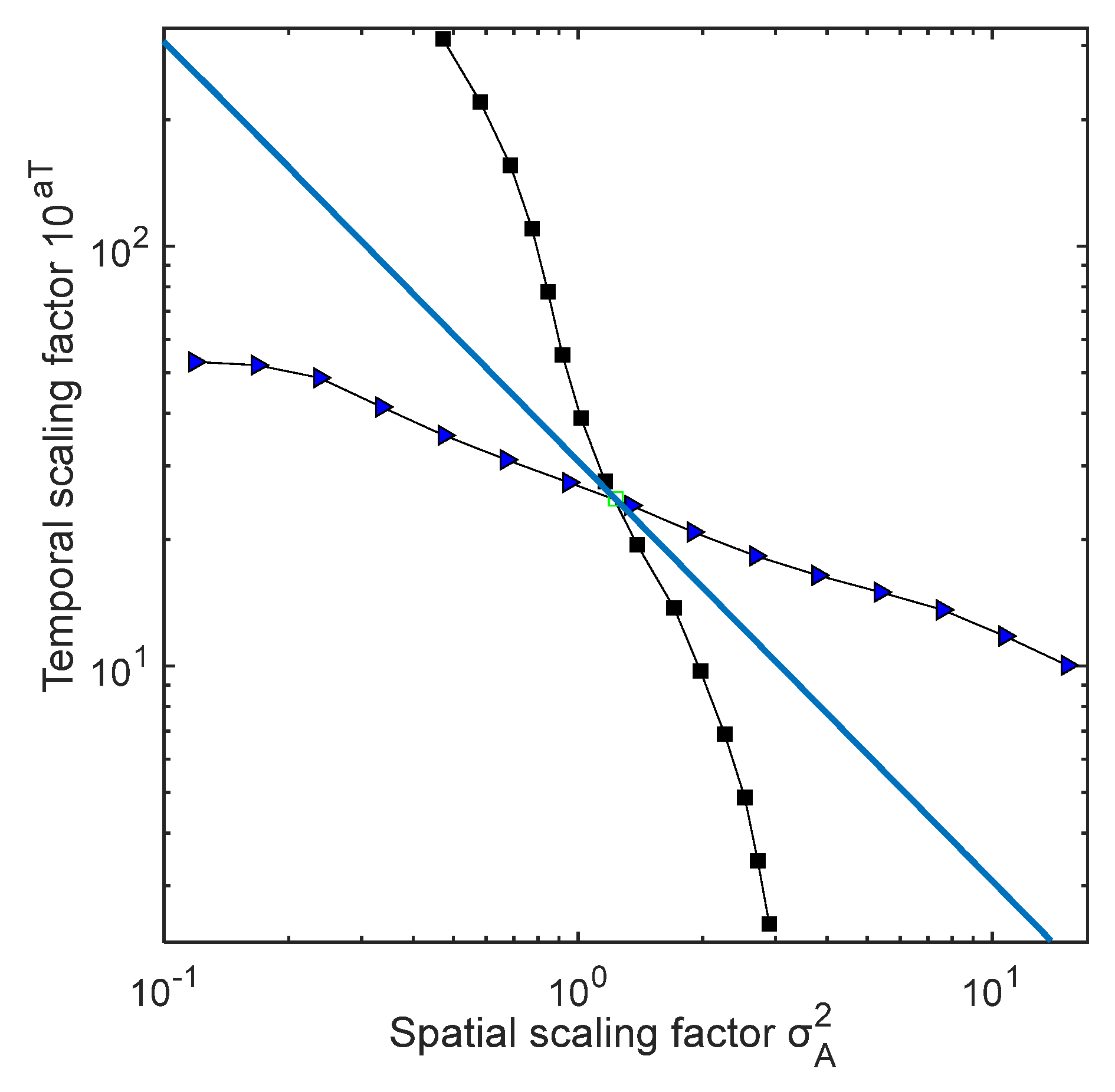
6.3. Space-Time Trade-Off

The study of synthetic catalogues provided empirical evidence for the existence of an intrinsic space-time trade-off in precursory seismicity. In [51]. The researchers noted that it is possible to make multiple identifications of Ψ with very different values of A P and T P for some major synthetic earthquakes. Similarly, we have observed multiple Ψ identifications for real major earthquakes. Generally, larger values of A P are associated with smaller values of T P , and vice versa. For example, an alternative identification of Ψ can be found for the Aegean Sea 2020 earthquake (Figure 12), which can be compared to that in Figure 1. The A P value in Figure 12 is 2.5 times larger, and the T P value 1.6 times smaller, than in Figure 1. Such a multiplicity of A P and T P values for individual mainshocks suggests that the space-time trade-off is an inherent feature of precursory seismicity.
The nature of the space-time trade-off has been further probed through fitting of the EEPAS time- and area-scaling parameters a T and σ A , respectively. In [53], a T and σ A were systematically controlled in such a way that the temporal and spatial scales varied by two orders of magnitude. As one of the parameters was varied, the other was refitted to a 20-year period of the New Zealand and California earthquake catalogues. The starting point was the optimal parameter set previously fitted to these catalogues [58]. The resulting curves of the temporal-scaling factor versus the spatial-scaling factor showed an even trade-off between time and area (Figure 13). Moreover, the refitted models all had information gains that were no more than 0.2 lower than that of the original optimal model, even though they were making use of precursors from widely different scales of time and space than the optimal model.
The space-time trade-off can be exploited to improve forecasting, by mixing models with alternative sets of parameters chosen from points along the line of even trade-off. In [53], using an arbitrary mixture of three models along the line was shown to increase the information gain in a testing period by up to 0.25 compared to that of the optimal individual model. The mixture was composed of the optimal individual model and two others formed by arbitrarily increasing and decreasing a T by 0.5 and adjusting σ A accordingly. More research is needed to develop a formal method for systematically incorporating the space–time trade-off into medium-term earthquake forecasts.
The space-time trade-off implies that for earthquakes with relatively long precursor times, we should expect relatively small precursory areas. If this statement stands for the Australian examples in Figure 2b, where T P values are large, the A P values are expected to be small relative to the fitted regression (Figure 2c). On the contrary, A P values are relatively large. This can be explained by interaction of three factors. These are (1) rate dependence of T P , (2) the space-time trade-off, and (3) the short length of the catalogue. Given the low seismicity rate in Australia, the observed T P values are shorter than expected. This is due to the limit imposed by the length of the catalogue on the observable T P . As a result, the T P values, although large relative to the regression, are not as large as they would be if identified from a much longer catalogue. Finally, the existence of space-time trade-off results in relatively large A P values corresponding to such small observed T P values.

7. Challenges in EEPAS Forecasting: A Journey from What We Know to What We Don’t

Since its introduction in 2004, EEPAS has been a successful forecasting model for well-catalogued regions including New Zealand [16,24,26,27,57,58,79], California [16,20,25,53,58], Japan [17,18,21,22,86], and Greece [19]. To address the limitations imposed by the input earthquake catalogues, EEPAS has undergone many revisions. As mentioned earlier, one milestone in the EEPAS improvement was compensation of the forecasts for missing precursory earthquakes in the time-lag between the end of the catalogue and the forecasting time-horizon. We have also learned how to compensate EEPAS forecasts for the limited record of precursory information before any target earthquake. Overall, the current version of the EEPAS is much better adapted to deal with the limitations of any earthquake catalogue than previously. However, there are still significant challenges and unknowns as outlined here.

7.1. Understanding the Physics behind the Ψ-Phenomenon

The Ψ-phenomenon and EEPAS model are empirically based. However, the Ψ-phenomenon can be identified as easily in synthetic catalogues as in real earthquake catalogues and the EEPAS model also works well in synthetic catalogues [51,82]. Synthetic catalogues are based on physical components such as fault networks, slip rates on faults, friction laws, and Coulomb stress calculations [85,87]. The earthquake generation process of each synthetic earthquake is in principle traced through the stress transfer between neighbouring faults. This leads to an eventual failure of the fault that produces the earthquake. Ideally, the origin of the Ψ-phenomenon should be explained by a similar physics-based concept. Such an understanding is likely to be helpful in guiding future refinements of the EEPAS model.

7.2. Incorporating Dependence on the Long-Term Earthquake Rate

We have learned from analysis of synthetic catalogues that the scale of the EEPAS time distribution is inversely proportional to the slip rate on faults. Slip rates are related to the long-term rate of the earthquakes that they generate [88]. Therefore, we should expect the scale of the EEPAS time distribution to be inversely related to the long-term earthquake rate.
If the spatial variability of the long-term earthquake rate is known, it can be incorporated into the EEPAS model using Equation (19). This is straight-forward and does not add to the number of fitted parameters in the model. The challenge is how to best estimate it from existing data sources [60]. The long-term earthquake rates can be estimated from smoothed seismicity, strain rates, faults and their slip rates, the location of plate boundaries, or some combinations of these. The main limitation is the restricted length of the available catalogue against which to test them.

7.3. A Three-Dimensional Version of EEPAS?

The EEPAS model at present only makes use of two spatial dimensions—latitude and longitude. All earthquakes within a chosen depth range are treated the same, regardless of their estimated hypocentral depths. The reason for this is primarily that depth determinations are often poorly constrained. In the New Zealand catalogue, many depths are fixed by analysts, rather than directly estimated, because of the difficulty of estimating depths using a 2D velocity model and the available seismograph network. We expect that the seismograph network will become denser over time and a comprehensive 3D velocity model [89] will be incorporated in the GeoNet earthquake locator. As a result, the precision of depth determinations will improve. Then, it will make sense to shift to three-dimensional distance determinations in the EEPAS model.

7.4. Target-Earthquake Oriented Compensation for Missing Precursors

We have shown how to compensate EEPAS for missing earthquakes with a fixed lead time. However, applying a fixed lead time is potentially wasteful of precious earthquake catalogue data. Ignoring the early earthquakes in a catalogue can adversely affect the forecasting of large earthquakes, which have very long precursor times. It is the largest earthquakes that we are ultimately most interested in forecasting, even though conformity to the Gutenberg-Richter law limits their contribution to the information gain.
The challenge is then to use as much of the past catalogue as possible and compensate the forecast of each target earthquake for the incompleteness of precursory contributions at each point in time, location, and magnitude. This is what we call “target-oriented” compensation. Shifting from a fixed lead time to target-oriented compensation would involve modifying Equations (13)–(16).
The incompleteness of precursory contributions for each target earthquake depends on the completeness of the catalogue in its vicinity in the period prior to its occurrence.

7.5. Accommodating Variable Incompleteness of the Earthquake Catalogue

Completeness of an earthquake catalogue varies with time, magnitude, and location depending on the network configuration and instrumentations [76]. Treatments of catalogue completeness can range from simple to elaborate. In the simplest approach, one might choose a starting time t 0 after which the input catalogue is approximately complete for all magnitudes above a minimum threshold m 0 , as illustrated in Figure 4. Target-oriented compensation could then be applied based on the lead time between t 0 and the time of each target earthquake. A more elaborate approach would be to estimate a magnitude-dependent starting time t 0 ( m ) at which the catalogue becomes complete for magnitude m > m 0 (see Figure 14). The lead time L ( m ) for a given target earthquake then varies with the input magnitude. Furthermore, one can also take into account the effect of spatial variations on the catalogue completeness, due to time-varying coverage of the region of interest by the seismic network.

7.6. Optimal Use of the Space-Time Trade-Off

The space-time trade-off of precursory seismicity presents opportunities to improve EEPAS forecasts by mixing models from points on the line of even trade-off, as previously demonstrated [53]. However, optimally incorporating the trade-off into the EEPAS model remains a challenge. The space-time trade-off imposes a relation between the fitted values a T and σ A . However, it may also affect other parameters, such as σ T .
It is undesirable to incorporate the trade-off subjectively. Ideally, a revised fitting process would automatically integrate contributions to the forecast from points along the line. This would require some reformulation of the model.

7.7. Development of a Global Forecasting Model

An important goal for the future is the development of a global EEPAS model. The aim is to forecast the largest earthquakes, e.g., M 7 , expected to occur anywhere in the world, with time horizons extending out to several decades, using a global catalogue. All factors now known to affect the EEPAS parameters—incompleteness of precursory earthquakes, the space-time trade-off, and dependence on long-term earthquake rates—need to be simultaneously addressed in a coherent way to develop such a global model.
The model would be regionally adjustable to accommodate variation in the earthquake rate and the space-time trade-off of precursory seismicity. It would also include compensation for incompleteness of precursory contributions. The earthquake occurrence rates vary by several orders of magnitude between plate-boundary regions and continental regions. The time distribution in the EEPAS model would therefore vary over a similarly wide range. This induces far more variability in completeness of precursory contributions than in regional catalogues that adds to the challenge. These complexities imply there is still some way to go to develop a global EEPAS model.

8. Conclusions

Over the past two decades, the EEPAS model has been progressively developed through empirical observation and statistical modelling. The motivation has always been to enhance its forecasting performance in terms of information gain. It has been tested in combination with a variety of independent earthquake forecasting models. This has led to the incorporation of EEPAS in public earthquake forecasting in New Zealand. Compensation of the model for temporal incompleteness of precursory contributions due to the time-lag has improved forecasting performance. For lower magnitude target earthquakes, it can extend the effective forecasting time horizon from a few months to a few decades. Moreover, compensation for the lead time can improve the forecasting performance for large earthquakes.
Studies on synthetic and real catalogues have revealed some of the EEPAS characteristics. One is the space-time trade-off of the precursor time and precursory area in the Ψ-phenomenon, which is reflected in the EEPAS time and area scaling parameters a T and σ A , respectively. Another is the effect of earthquake rate dependence on the time distribution of precursory seismicity. This was verified in the Ψ-phenomenon but has still to be fully realized in the EEPAS model.
All the modifications made to EEPAS, together with dynamic improvement of seismic networks and computational resources, are smoothing the path to development of a global EEPAS model. Despite these advances, challenges remain in developing an enhanced physical understanding of the Ψ-phenomenon, and in coherently integrating the known effects on scaling and compensation for missing precursory earthquakes into the EEPAS model. Addressing these challenges motivates future research in this area.

Author Contributions

Conceptualization, D.A.R., S.J.R. and A.C.; methodology, D.A.R.; software, D.A.R. and S.J.R.; formal analysis, D.A.R.; writing—original draft preparation, D.A.R. and S.J.R.; writing—review and editing, D.A.R., S.J.R. and A.C. All authors have read and agreed to the published version of the manuscript.

Funding

This project was supported by the New Zealand Ministry of Business, Innovation and Employment (MBIE) through the Hazards and Risks Management programme (Strategic Science Investment Fund, contract C05X1702).

Data Availability Statement

Data for the M6.7 Aegean Sea earthquake 2020 and precursory sequence are from the International Seismological Centre (ISC) earthquake catalogue. Available online at https://doi.org/10.31905/D808B830 (accessed on 21 May 2022). The New Zealand earthquake catalogue data came primarily from GeoNet. Available online at: http://www.geonet.org.nz (accessed on 30 September 2021). The Adjusted Magnitude (AMC) catalogue is derived from the Geonet New Zealand earthquake catalogue. It is available online at https://doi.org/10.21420/tap4-5s59 (accessed on 19 September 2022).

Acknowledgments

We thank the three anonymous reviewers for their constructive comments, which have helped in revision of the manuscript. We acknowledge the New Zealand GeoNet project and its sponsors EQC, GNS Science, LINZ, NEMA and MBIE for providing the data used in this study.

Conflicts of Interest

The authors declare no conflict of interest. The funders had no role in the design of the study; in the collection, analyses, or interpretation of data; in the writing of the manuscript, or in the decision to publish the results.

References

  1. Vere-Jones, D.; Ben-Zion, Y.; Zúñiga, R. Statistical Seismology. Pure Appl. Geophys. 2005, 162, 1023–1026. [Google Scholar] [CrossRef]
  2. Vere-Jones, D. Foundations of Statistical Seismology. Pure Appl. Geophys. 2010, 167, 645–653. [Google Scholar] [CrossRef]
  3. Omori, F. On the aftershocks of earthquakes. J. Coll. Sci. Imp. Univ. Tokyo 1885, 7, 111–200. [Google Scholar]
  4. Utsu, T.; Ogata, Y. The centenary of the Omori formula for a decay law of aftershock activity. J. Phys. Earth 1995, 43, 1–33. [Google Scholar] [CrossRef]
  5. Gutenberg, B.; Richter, C.F. Frequency of earthquakes in California. Bull. Seismol. Soc. Am. 1944, 34, 185–188. [Google Scholar] [CrossRef]
  6. Lindman, M.; Lund, B.; Roberts, R.; Jonsdottir, K. Physics of the Omori law: Inferences from interevent time distributions and pore pressure diffusion modeling. Tectonophysics 2006, 424, 209–222. [Google Scholar] [CrossRef]
  7. Hainzl, S.; Marsan, D. Dependence of the Omori-Utsu law parameters on main shock magnitude: Observations and modeling. J. Geophys. Res. Solid Earth 2008, 113, B10309. [Google Scholar] [CrossRef]
  8. Guglielmi, A.V. Interpretation of the Omori law. Izv. Phys. Solid Earth 2016, 52, 785–786. [Google Scholar] [CrossRef]
  9. Faraoni, V. Lagrangian formulation of Omori’s law and analogy with the cosmic Big Rip. Eur. Phys. J. C 2020, 80, 445. [Google Scholar] [CrossRef]
  10. Mogi, K. Magnitude-Frequency Relation for Elastic Shocks Accompanying Fractures of Various Materials and Some Related problems in Earthquakes (2nd Paper). Bull. Earthq. Res. Inst. Univ. Tokyo 1963, 40, 831–853. [Google Scholar]
  11. Schorlemmer, D.; Wiemer, S.; Wyss, M. Variations in earthquake-size distribution across different stress regimes. Nature 2005, 437, 539–542. [Google Scholar] [CrossRef] [PubMed]
  12. Amitrano, D. Variability in the power-law distributions of rupture events. Eur. Phys. J. Spec. Top. 2012, 205, 199–215. [Google Scholar] [CrossRef] [Green Version]
  13. Varotsos, P.A.; Sarlis, N.V.; Skordas, E.S.; Christopoulos, S.-R.G.; Lazaridou-Varotsos, M.S. Identifying the occurrence time of an impending mainshock: A very recent case. Earthq. Sci. 2015, 28, 215–222. [Google Scholar] [CrossRef]
  14. Evison, F.; Rhoades, D. Precursory scale increase and long-term seismogenesis in California and Northern Mexico. Ann. Geophys. 2002, 45, 479–495. [Google Scholar] [CrossRef]
  15. Evison, F.F.; Rhoades, D.A. Demarcation and Scaling of Long-term Seismogenesis. Pure Appl. Geophys. 2004, 161, 21–45. [Google Scholar] [CrossRef]
  16. Rhoades, D.A.; Evison, F.F. Long-range earthquake forecasting with every earthquake a precursor according to scale. Pure Appl. Geophys. 2004, 161, 47–72. [Google Scholar] [CrossRef]
  17. Rhoades, D.A.; Evison, F.F. Test of the EEPAS Forecasting Model on the Japan earthquake catalogue. Pure Appl. Geophys. 2005, 162, 1271–1290. [Google Scholar] [CrossRef]
  18. Rhoades, D.A.; Evison, F.F. The EEPAS forecasting model and the probability of moderate-to-large earthquakes in central Japan. Tectonophysics 2006, 417, 119–130. [Google Scholar] [CrossRef]
  19. Console, R.; Rhoades, D.A.; Murru, M.; Evison, F.F.; Papadimitriou, E.E.; Karakostas, V.G. Comparative performance of time-invariant, long-range and short-range forecasting models on the earthquake catalogue of Greece. J. Geophys. Res. Solid Earth 2006, 111, B09304. [Google Scholar] [CrossRef]
  20. Rhoades, D.A. Application of the EEPAS model to forecasting earthquakes of moderate magnitude in southern California. Seismol. Res. Lett. 2007, 78, 110–115. [Google Scholar] [CrossRef]
  21. Rhoades, D.A. Application of a long-range forecasting model to earthquakes in the Japan mainland testing region. Earth Planets Space 2011, 63, 197–206. [Google Scholar] [CrossRef]
  22. Rhoades, D.A.; Somerville, P.G.; Somerville, F.; de Oliveira, D.; Thio, H.K. Effect of tectonic setting on the fit and performance of a long-range earthquake forecasting model. Res. Geophys. 2012, 2, 13–23. [Google Scholar] [CrossRef] [Green Version]
  23. Zechar, J.D.; Schorlemmer, D.; Liukis, M.; Yu, J.; Euchner, F.; Maechling, P.J.; Jordan, T.H. The Collaboratory for the Study of Earthquake Predictability perspective on computational earthquake science. Concurr. Comput. Pract. Exp. 2010, 22, 1836–1847. [Google Scholar] [CrossRef]
  24. Gerstenberger, M.C.; Rhoades, D.A. New Zealand earthquake forecast testing centre. In Seismogenesis and Earthquake Forecasting: The Frank Evison Volume II; Springer: Berlin/Heidelberg, Germany, 2010; pp. 23–38. [Google Scholar]
  25. Schneider, M.; Clements, R.; Rhoades, D.; Schorlemmer, D. Likelihood- and residual-based evaluation of medium-term earthquake forecast models for California. Geophys. J. Int. 2014, 198, 1307–1318. [Google Scholar] [CrossRef]
  26. Rhoades, D.A.; Christophersen, A.; Gerstenberger, M.C.; Liukis, M.; Silva, F.; Marzocchi, W.; Werner, M.J.; Jordan, T.H. Highlights from the first ten years of the New Zealand Earthquake Forecast Testing Center. Seismol. Res. Lett. 2018, 89, 1229–1237. [Google Scholar] [CrossRef]
  27. Gerstenberger, M.; Rhoades, D.; Litchfield, N.; Van Dissen, R.; Abbot, E.; Goded, T.; Christophersen, A.; Bannister, S.; Barrell, D.; Bruce, Z.; et al. The Kaikoura Seismic Hazard Model. N. Z. J. Geol. Geophys. 2022. in revision. [Google Scholar]
  28. Gerstenberger, M.; McVerry, G.; Rhoades, D.; Stirling, M. Seismic Hazard Modeling for the Recovery of Christchurch. Earthq. Spectra 2014, 30, 17–29. [Google Scholar] [CrossRef]
  29. Rhoades, D.A.; Liukis, M.; Christophersen, A.; Gerstenberger, M.C. Retrospective tests of hybrid operational earthquake forecasting models for Canterbury. Geophys. J. Int. 2015, 204, 440–456. [Google Scholar] [CrossRef]
  30. Evison, F.F. The precursory earthquake swarm. Phys. Earth Planet. Inter. 1977, 15, 19–23. [Google Scholar] [CrossRef]
  31. Evison, F.F. Precursory seismic sequences in New Zealand. N. Z. J. Geol. Geophys. 1977, 20, 129–141. [Google Scholar] [CrossRef]
  32. Evison, F.F. Fluctuations of seismicity before major earthquakes. Nature 1977, 266, 710–712. [Google Scholar] [CrossRef]
  33. Evison, F. Multiple earthquake events at moderate-to-large magnitudes in Japan. J. Phys. Earth 1981, 29, 327–339. [Google Scholar] [CrossRef]
  34. Evison, F. Generalised Precursory Swarm Hypothesis. J. Phys. Earth 1982, 30, 155–170. [Google Scholar] [CrossRef]
  35. Rikitake, T. Earthquake precursors. Bull. Seismol. Soc. Am. 1975, 65, 1133–1162. [Google Scholar] [CrossRef]
  36. Rikitake, T. Classification of earthquake precursors. Tectonophysics 1979, 54, 293–309. [Google Scholar] [CrossRef]
  37. Rikitake, T. Earthquake Forecasting and Warning; Dordrecht Boston: D. Reidel; Hingham, Mass.: Sold and distributed in the U.S.A. and Canada by Kluwer Boston; Center for Academic Publications Japan: Tokyo, Japan, 1982. [Google Scholar]
  38. Rhoades, D.A.; Evison, F.F. Long-range earthquake forecasting based on a single predictor. Geophys. J. Int. 1979, 59, 43–56. [Google Scholar] [CrossRef]
  39. Evison, F.F.; Rhoades, D.A. The precursory earthquake swarm in New Zealand: Hypothesis tests. N. Z. J. Geol. Geophys. 1993, 36, 51–60. [Google Scholar] [CrossRef]
  40. Rhoades, D.A.; Evison, F.F. Long-range earthquake forecasting based on a single predictor with clustering. Geophys. J. Int. 1993, 113, 371–381. [Google Scholar] [CrossRef]
  41. Evison, F.F.; Rhoades, D.A. The precursory earthquake swarm in New Zealand: Hypothesis tests. N. Z. J. Geol. Geophys. 1997, 40, 537–547. [Google Scholar] [CrossRef]
  42. Evison, F.F.; Rhoades, D.A. Long-term seismogenic process for major earthquakes in subduction zones. Phys. Earth Planet. Inter. 1998, 108, 185–199. [Google Scholar] [CrossRef]
  43. Evison, F.F.; Rhoades, D.A. The precursory earthquake swarm and the inferred precursory quarm. N. Z. J. Geol. Geophys. 1999, 42, 229–236. [Google Scholar] [CrossRef]
  44. Evison, F.F.; Rhoades, D.A. The precursory earthquake swarm in Japan: Hypothesis test. Earth Planets Space 1999, 51, 1267–1277. [Google Scholar] [CrossRef]
  45. Evison, F.; Rhoades, D. The precursory earthquake swarm in Greece. Ann. Geophys. 2000, 43, 991–1009. [Google Scholar] [CrossRef]
  46. Evison, F.; Rhoades, D. Model of long-term seismogenesis. Ann. Geophys. 2001, 44, 81–93. [Google Scholar] [CrossRef]
  47. Ogata, Y. Statistical model for standard seismicity and detection of anomalies by residual analysis. Tectonophysics 1989, 169, 159–174. [Google Scholar] [CrossRef]
  48. Ogata, Y. Space-Time Point-Process Models for Earthquake Occurrences. Ann. Inst. Stat. Math. 1998, 50, 379–402. [Google Scholar] [CrossRef]
  49. Evison, F.; Rhoades, D. Multiple-mainshock events and long-term seismogenesis in Italy and New Zealand. N. Z. J. Geol. Geophys. 2005, 48, 523–536. [Google Scholar] [CrossRef]
  50. Papadimitriou, E.E.; Evison, F.F.; Rhoades, D.A.; Karakostas, V.G.; Console, R.; Murru, M. Long-term seismogenesis in Greece: Comparison of the evolving stress field and precursory scale increase approaches. J. Geophys. Res. Solid Earth 2006, 111, B05318. [Google Scholar] [CrossRef]
  51. Christophersen, A.; Rhoades, D.A.; Colella, H.V. Precursory seismicity in regions of low strain rate: Insights from a physics-based earthquake simulator. Geophys. J. Int. 2017, 209, 1513–1525. [Google Scholar] [CrossRef]
  52. Rhoades, D.A.; Rastin, S.J.; Christophersen, A. The effect of catalogue lead time on medium-term earthquake forecasting with application to New Zealand data. Entropy 2020, 22, 1264. [Google Scholar] [CrossRef]
  53. Rastin, S.J.; Rhoades, D.A.; Christophersen, A. Space–time trade-off of precursory seismicity in New Zealand and California revealed by a medium-term earthquake forecasting model. Appl. Sci. 2021, 11, 10215. [Google Scholar] [CrossRef]
  54. Jackson, D.D.; Kagan, Y.Y. Testable Earthquake Forecasts for 1999. Seismol. Res. Lett. 1999, 70, 393–403. [Google Scholar] [CrossRef]
  55. Daley, D.J.; Vere-Jones, D. An Introduction to the Theory of Point Processes, 2nd ed.; Springer: Berlin/Heidelberg, Germany, 2008; Volume II. [Google Scholar]
  56. Ogata, Y.; Zhuang, J. Space–time ETAS models and an improved extension. Tectonophysics 2006, 413, 13–23. [Google Scholar] [CrossRef]
  57. Rhoades, D.A.; Christophersen, A. Time-varying probabilities of earthquake occurrence in central New Zealand based on the EEPAS model compensated for time-lag. Geophys. J. Int. 2019, 219, 417–429. [Google Scholar] [CrossRef]
  58. Rhoades, D.A. Mixture Models for Improved Earthquake Forecasting with Short-to-Medium Time Horizons. Bull. Seismol. Soc. Am. 2013, 103, 2203–2215. [Google Scholar] [CrossRef]
  59. Rhoades, D.A.; Schorlemmer, D.; Gerstenberger, M.C.; Christophersen, A.; Zechar, J.D.; Imoto, M. Efficient testing of earthquake forecasting models. Acta Geophys. 2011, 59, 728–747. [Google Scholar] [CrossRef]
  60. Rastin, S.J.; Rhoades, D.A.; Rollins, C.; Gerstenberger, M.C. How Useful Are Strain Rates for Estimating the Long-Term Spatial Distribution of Earthquakes? Appl. Sci. 2022, 12, 6804. [Google Scholar] [CrossRef]
  61. Hurvich, C.M.; Tsai, C.-L. Regression and time series model selection in small samples. Biometrika 1989, 76, 297–307. [Google Scholar] [CrossRef]
  62. Rhoades, D.A.; Gerstenberger, M.C. Mixture models for improved short-term earthquake forecasting. Bull. Seismol. Soc. Am. 2009, 99, 636–646. [Google Scholar] [CrossRef]
  63. Rhoades, D.A. Long-range earthquake forecasting allowing for aftershocks. Geophys. J. Int. 2009, 178, 244–256. [Google Scholar] [CrossRef]
  64. Rhoades, D.A.; Gerstenberger, M.C.; Christophersen, A. Development, Installation and Testing of New Models in the New Zealand Earthquake Forecast Testing Centre; CR2010-253; GNS Science: Lower Hutt, New Zealand, 2010; 55p. [Google Scholar]
  65. Rastin, S.J.; Rhoades, D.; Christophersen, A. Space-time trade-off of precursory seismicity in the EEPAS medium-term forecasting model optimized for New Zealand earthquakes. In Proceedings of the AGU 2020 Fall Meeting, virtual, 1–17 December 2020. [Google Scholar]
  66. Gerstenberger, M.C.; Wiemer, S.; Jones, L.M.; Reasenberg, P.A. Real-time forecasts of tomorrow’s earthquakes in California. Nature 2005, 435, 328–331. [Google Scholar] [CrossRef] [PubMed]
  67. Gutenberg, B.; Richter, C.F. Seismicity of the Earth and Associated Phenomena; Princeton, N.J., Ed.; Princeton University Press: Princeton, NJ, USA, 1954. [Google Scholar]
  68. Utsu, T. A statistical study on the occurrence of aftershocks. Geophys. Mag. 1961, 30, 521–605. [Google Scholar]
  69. Gledhill, K.; Ristau, J.; Reyners, M.; Fry, B.; Holden, C. The Darfield (Canterbury) earthquake of September 2010: Preliminary seismological report. Bull. N. Z. Soc. Earthq. Eng. 2010, 43, 215–221. [Google Scholar]
  70. Kaiser, A.; Holden, C.; Beavan, J.; Beetham, D.; Benites, R.; Celentano, A.; Collett, D.; Cousins, J.; Cubrinovski, M.; Dellow, G.; et al. The Mw 6.2 Christchurch earthquake of February 2011: Preliminary report. N. Z. J. Geol. Geophys. 2012, 55, 67–90. [Google Scholar] [CrossRef]
  71. Yan, W.; Galloway, W. Rethinking Resilience, Adaptation and Transformation in a Time of Change; Springer International Publishing: Berlin, Germany, 2017. [Google Scholar]
  72. Stirling, M.; McVerry, G.H.; Gerstenberger, M.C.; Litchfield, N.J.; Van Dissen, R.J.; Berryman, K.R.; Barnes, P.; Wallace, L.M.; Villamor, P.; Langridge, R.M.; et al. National Seismic Hazard Model for New Zealand: 2010 Update. Bull. Seismol. Soc. Am. 2012, 102, 1514–1542. [Google Scholar] [CrossRef] [Green Version]
  73. Gerstenberger, M.C.; Rhoades, D.A.; McVerry, G.H. A hybrid time-dependent probabilistic seismic-hazard model for Canterbury, New Zealand. Seismol. Res. Lett. 2016, 87, 1311–1318. [Google Scholar] [CrossRef]
  74. Meletti, C.; Galadini, F.; Valensise, G.; Stucchi, M.; Basili, R.; Barba, S.; Vannucci, G.; Boschi, E. A seismic source zone model for the seismic hazard assessment of the Italian territory. Tectonophysics 2008, 450, 85–108. [Google Scholar] [CrossRef]
  75. Kaiser, A.; Balfour, N.; Fry, B.; Holden, C.; Litchfield, N.; Gerstenberger, M.; D’Anastasio, E.; Horspool, N.; McVerry, G.; Ristau, J.; et al. The 2016 Kaikōura, New Zealand, earthquake: Preliminary seismological report. Seismol. Res. Lett. 2017, 88, 727–739. [Google Scholar] [CrossRef]
  76. Havskov, J.; Ottemoller, L. Routine Data Processing in Earthquake Seismology: With Sample Data, Exercises and Software; Springer: Dordrecht, The Netherlands, 2010. [Google Scholar]
  77. Rastin, S.J.; Unsworth, C.P.; Gledhill, K.R.; McNamara, D.E. A detailed noise characterization and sensor evaluation of the North Island of New Zealand using the PQLX data quality control system. Bull. Seismol. Soc. Am. 2012, 102, 98–113. [Google Scholar] [CrossRef]
  78. Bormann, P.; Wielandt, E. Seismic Signals and Noise. In New Manual of Seismological Observatory Practice 2 (NMSOP2); Deutsches GeoForschungsZentrum GFZ: Potsdam, Germany, 2013. [Google Scholar] [CrossRef]
  79. Rastin, S.J.; Rhoades, D.A.; Rollins, C.; Gerstenberger, M.C.; Christophersen, A.; Thingbaijam, K.K.S. Spatial Distribution of Earthquake Occurrence for the New Zealand National Seismic Hazard Model Revision, GNS Science Report; SR2021-51; GNS Science: Lower Hutt, New Zealand, 2022. [Google Scholar]
  80. Christophersen, A.; Bourgignon, S.; Rhoades, D.A.; Allen, T.I.; Salichon, J.; Ristau, J.; Gerstenberger, M. Consistent Magnitudes over Time for the Revision of the New Zealand National Seismic Hazard Model, GNS Science Report; SR2021-42; GNS Science: Lower Hutt, New Zealand, 2022. [Google Scholar] [CrossRef]
  81. Rhoades, D.A. Lessons and Questions from Thirty Years of Testing the Precursory Swarm Hypothesis. Pure Appl. Geophys. 2010, 167, 629–644. [Google Scholar] [CrossRef]
  82. Rhoades, D.A.; Robinson, R.; Gerstenberger, M.C. Long-range predictability in physics-based synthetic earthquake catalogues. Geophys. J. Int. 2011, 185, 1037–1048. [Google Scholar] [CrossRef]
  83. Robinson, R.; Van Dissen, R.R.; Litchfield, N. Using synthetic seismicity to evaluate seismic hazard in the Wellington region, New Zealand. Geophys. J. Int. 2011, 187, 510–528. [Google Scholar] [CrossRef]
  84. Robinson, R.; Benites, R. Synthetic seismicity models for the Wellington Region, New Zealand: Implications for the temporal distribution of large events. J. Geophys. Res. Solid Earth 1996, 101, 27833–27844. [Google Scholar] [CrossRef]
  85. Richards-Dinger, K.; Dieterich, J.H. RSQSim Earthquake Simulator. Seismol. Res. Lett. 2012, 83, 983–990. [Google Scholar] [CrossRef]
  86. Imoto, M.; Rhoades, D.A. Seismicity models of moderate earthquakes in Kanto, Japan utilizing multiple predictive parameters. Pure Appl. Geophys. 2010, 167, 831–843. [Google Scholar] [CrossRef]
  87. Robinson, R.; Benites, R. Upgrading a synthetic seismicity model for more realistic fault ruptures. Geophys. Res. Lett. 2001, 28, 1843–1846. [Google Scholar] [CrossRef]
  88. Scholz, C.H. The Mechanics of Earthquakes and Faulting, 3rd ed.; Cambridge University Press: Cambridge, UK, 2019. [Google Scholar]
  89. Eberhart-Phillips, D.; Reyners, M.; Bannister, S.; Chadwick, M.; Ellis, S. Establishing a versatile 3-D seismic velocity model for New Zealand. Seismol. Res. Lett. 2010, 81, 992–1000. [Google Scholar] [CrossRef]
Figure 1. An identification of the Ψ-phenomenon for the M6.7 Aegean Sea earthquake of 30 October 2020. (a) Epicenters of the precursory seismicity, mainshocks, and aftershocks, shown within the precursory area A P (rectangle). (b) Magnitude versus time of prior and precursory earthquakes with the onset of Ψ in 1992. There were no earthquakes prior to the onset. M m is the main shock magnitude; M P   is the precursor magnitude—the average magnitude of the three largest precursory earthquakes. (c) Changes in cumag with time. Dashed lines show the precursory increase in seismicity rate. The protractor translates the cumag slope into seismicity rate in magnitude units per year (M.U. yr–1). T P is precursor time. Data is from the ISC catalogue of earthquakes with magnitude M ≥ 4.5, starting September 1972. M P = 5.6; M m = 6.7; T P = 10,220 days; A P = 3203 km2.
Geosciences 12 00349 g001
Figure 2. Ψ- Predictive-scaling relations between (a) mainshock and precursor magnitudes M m and M P ; (b) precursor time T P and M P ; and (c) precursory area A P and M P , as fitted to 47 examples of Ψ [15]. The data plotted include these original 47 examples from California and northern Mexico, Japan, Greece and northwest Turkey and New Zealand; as well as 24 further examples, identified in subsequent references [49,50,51,52,53], from Italy, New Zealand, Greece, Australia, and California. The Aegean Sea 2020 earthquake (Figure 1) is plotted with large triangles.
Geosciences 12 00349 g002
Figure 3. Probability densities of a precursory earthquake contribution to the earthquake occurrence rate density. Joint time and magnitude density (Equations (3) and (4)) for precursor with (a) mi = 4.5, (c) mi = 5.5; Spatial density (Equation (5)) for precursor with (b) mi = 4.5, (d) mi = 5.5. Densities are scaled relative to their maximum values. The parameters are from the EEPAS_0F model for New Zealand, discussed in Section 5.1 below.
Geosciences 12 00349 g003
Figure 4. Diagram illustrating warm-up, fitting, and testing periods; lead time and time-lag associated with a particular forecasting time horizon.
Geosciences 12 00349 g004
Figure 5. Illustrating the Kaikoura hybrid forecasting model, with the medium-term component supplied by EEPAS. Short-term, medium-term and long-term components and the Kaikoura hybrid model forecast (the maximum of the three components) at magnitude M L 5.0 for the two-month period commencing 26 June 2017. The earthquake occurrence rate density is relative to a reference (RTR) model in which one earthquake per year is expected to exceed any magnitude m in an area of 10 m km2.
Geosciences 12 00349 g005
Figure 6. Completeness of precursory earthquake contributions as a function of (a,b) time-lag for fixed lead time and (c,d) lead time for fixed time-lag for selected target magnitudes for parameters in Table 3.
Geosciences 12 00349 g006
Figure 7. Maps of New Zealand showing CSEP testing region (dashed inner polygon) and search region (dotted outer polygon) with (a) earthquakes M > 2.95 from 1951 to 2020 (blue dots) and (b) earthquakes M > 4.95 from 2006 to 2020 (red circles), including the target set of 147 earthquakes within the testing region. Earthquakes are shallow (depth ≤ 40 km) and were extracted from the AMC catalogue.
Geosciences 12 00349 g007
Figure 8. Completeness of precursory earthquake contributions as a function of time-lag and target magnitude for EEPAS_1F fitted to the AMC catalogue.
Geosciences 12 00349 g008
Figure 9. Fitted mixing parameter ω for time-lags ranging from 1 to 20 years for LEEPAS_1F model fitted to the AMC catalogue.
Geosciences 12 00349 g009
Figure 10. Information gains per earthquake (IG) of LEEPAS_1F fitted to the AMC catalogue over PPE with 95% confidence intervals.
Geosciences 12 00349 g010
Figure 11. Diagram illustrating forecasting with a fixed lead time L, highlighting lost information for target earthquakes (EQ1, EQ2 and EQ3) and for forecasting ahead beyond the end of the catalogue.
Geosciences 12 00349 g011
Figure 12. Alternative identification of the Ψ-phenomenon for the M6.7 Aegean Sea earthquake of 30 October 2020. (a) Epicenters of the precursory seismicity, mainshocks, and aftershocks. The rectangle containing them is the precursory area A P . (b) Magnitude versus time of prior and precursory earthquakes with the onset of Ψ in 2003. Dashed lines show precursory increase in magnitude level. M m is main shock magnitude; M P is precursor magnitude—the average magnitude of the three largest precursory earthquakes. (c) Changes in cumag with time. Dashed lines show precursory increase in seismicity rate. The protractor translates the cumag slope into seismicity rate in magnitude units per year (M.U. yr–1). T P is precursor time. Data is from the ISC catalogue of earthquakes with magnitude M ≥ 4.5, starting September 1972. M P = 5.7; M m = 6.7; T P = 6392 days; A P = 8091 km2.
Geosciences 12 00349 g012
Figure 13. Trade-off of spatial and temporal scaling factors σ A 2 and 10 a T , respectively, revealed by the fit of the EEPAS model for New Zealand with controlled values of σ A (blue triangles) and a T (black squares). The straight line with a slope of −1 represents an even trade-off between space and time. Taken from [53].
Geosciences 12 00349 g013
Figure 14. Diagram illustrating variable starting times t 0 ( m ) at which the catalogue is complete for input magnitudes m > m 0 and the resulting variable lead times L ( m ) at the time when a target earthquake occurs.
Geosciences 12 00349 g014
Table 1. Terminology used for Medium-Term Forecasting by EEPAS.
TermDescriptionReference
Fitting PeriodSubset of a catalogue used for carrying out parameter fitting.[16]
Testing PeriodSubset of a catalogue, separate from the fitting period, used for independent testing without further parameter adjustment.[16]
Warm-up eriodSubset of a catalogue providing information on precursory earthquakes and earthquake rates prior to the fitting period. This provides initial required data for the background component, as well as the time-varying component of EEPAS.[51]
Target EarthquakesEarthquakes with hypocenters within the region of surveillance and time origins in the fitting or testing periods or the future and magnitudes greater than a chosen threshold, e.g., M > 4.95.[19]
Precursory EarthquakesEarthquakes with hypocenters within a search region encompassing the region of surveillance with time origins covered by the catalogue and magnitudes greater than the input magnitude threshold, e.g., M > 2.95.[16]
Lead TimeLength of time from start of catalogue to time of occurrence of a target earthquake.[52]
DelayTime interval between when an earthquake occurs and the earliest time at which it is allowed to contribute to a forecast (e.g., 50 days).[16]
Time-lagIn fitting and testing: sometimes used as a synonym for “Delay”. In forecasting: the time interval between the end of the catalogue and the time for which a forecast is made (e.g., 5 years).[57]
Forecasting Time HorizonDepending on context, this can mean a future time or the most distant future time for which a forecast is made. It can also refer to the time-lag associated with such a forecast.[58]
Table 2. EEPAS versions at a glance.
VersionMathematical DescriptionReference
Standard EEPAS λ EEPAS   ( t , m , x , y ) = μ λ P P E ( t , m , x , y ) + t i t 0 , m i m 0 η ( m i ) λ i ( t , m , x , y )
λ i ( t , m , x , y ) = w i f ( t | t i , m i ) g ( m | m i ) h ( x , y | x i , y i , m i )
λ P P E ( t , m , x , y ) : Background rate density
[16,17,18]
STEP-EEPAS mixture λ SE   ( t , m , x , y ) = ( 1 r )   λ STEP ( t , m , x , y ) + r λ EEPAS ( t , m , x , y )
r :   0   r   1 .
[62]
EEPAS with aftershocks λ EAS   ( t , m , x , y ) = λ EEPAS ( t , m , x , y ) + λ A S ( t , m , x , y ) [63]
Earthquake Rate Dependent EEPAS (ERDEEP) a T ( j ) = a T c ρ log ρ ( j ) ;
σ A ( j ) = σ A ρ ( j ) c ρ 2
where   ρ ( j ) is rate in cell j.
[64]
Janus Model:
EEPAS-ETAS mixture
λ JANUS ( t , m , x , y ) = ( 1 q )   λ EEPAS ( t , m , x , y ) + q λ ETAS ( t , m , x , y )
q :   0   q 1.
[58]
EEPAS Compensated for Time-Lag (LEEPAS) λ LEEPAS ( t , m , x , y ) = ω λ A ( t , m , x , y ) + ( 1 ω ) λ B ( t , m , x , y ) .
ω :   0     ω   1 .
[57]
Fixed Lead Time EEPAS (FLEEPAS) λ FLEEPAS   ( t , m , x , y ) = μ λ P P E ( t , m , x , y ) + t i t L , m i m 0 η ( m i ) λ i ( t , m , x , y ) [52,65]
Fixed Lead Time Compensated EEPAS (FLCEEPAS) λ FLCEEPAS ( t , m , x , y ) = φ λ A ( t , m , x , y ) + ( 1 φ ) λ B ( t , m , x , y ) .
φ: 0 ≤ φ ≤ 1.
[52,65]
Table 3. EEPAS_0F model parameters for New Zealand (from [58]).
ParameterEEPAS_0F
m 0 2.95 *
m c 4.95 *
m m a x 10.05 *,!
b G R 1.16
a M 1.10
b M 1.0 *
σ M 0.39
a T 1.71
b T 0.39
σ T 0.60
b A 0.36
σ A 1.63
μ 2.2 × 10 4
* Fixed. Fitted. ! Standard threshold used for CSEP models.
Table 4. PPE (background) and EEPAS (time-varying) model parameters fitted to 2006–2020 of the AMC catalogue.
ParameterModelFitted ValueFitting Range
aPPE0.55unconstrained
dPPE5.26 (km)>1
sPPE2.4 × 10−12unconstrained
aMEEPAS1.001.0–2.0
bMEEPAS1.00 *NA
σMEEPAS0.200.2–0.5
aTEEPAS1.971.0–2.0
bTEEPAS0.350.3–0.7
σTEEPAS0.200.2–0.5
bAEEPAS0.590.3–0.7
σAEEPAS0.510.5–10
µEEPAS0.360.0–0.5
*: Fixed parameter.
Publisher’s Note: MDPI stays neutral with regard to jurisdictional claims in published maps and institutional affiliations.

