Article

Spatio-Seasonal Hypoxia/Anoxia Dynamics and Sill Circulation Patterns Linked to Natural Ventilation Drivers, in a Mediterranean Landlocked Embayment: Amvrakikos Gulf, Greece

by
Nikos Georgiou
1,*,
Elias Fakiris
1,
Constantin Koutsikopoulos
2,
George Papatheodorou
1,
Dimitris Christodoulou
1,
Xenophon Dimas
1,
Maria Geraga
1,
Zacharias G. Kapellonis
3,
Konstantinos-Marios Vaziourakis
4,
Alexandra Noti
1,
Dimitra Antoniou
1 and
George Ferentinos
1
1
Laboratory of Marine Geology and Physical Oceanography, Department of Geology, University of Patras, 26500 Rio Patras, Greece
2
Department of Biology, University of Patras, 26500 Rio Patras, Greece
3
Hellenic Centre for Marine Research, Institute of Marine Biological Resources and Inland Waters, 576A Vouliagmenis Ave., 16452 Athens, Greece
4
Department of Ecology and Genetics/Limnology, Uppsala University, 75236 Uppsala, Sweden
*
Author to whom correspondence should be addressed.
Geosciences 2021, 11(6), 241; https://doi.org/10.3390/geosciences11060241
Submission received: 12 March 2021 / Revised: 31 May 2021 / Accepted: 1 June 2021 / Published: 3 June 2021
(This article belongs to the Section Geophysics)

Abstract

:
Amvrakikos Gulf is a Mediterranean landlocked, fjord-like embayment and marine protected area suffering from natural, human-induced hypoxia/anoxia and massive fish mortality events. Seasonal marine geophysical and oceanographic surveys were conducted focusing on the water-circulation patterns at the sill and the spatial-seasonal distribution of dissolved oxygen (DO) in the gulf. Detailed surveys at the sill, the only communication route between the gulf and the open sea, revealed a two-layer water circulation pattern (top brackish outflow–bottom seawater inflow) and the role of the tide in the daily water exchange. Statistical analysis of the known natural drivers of DO distribution (density difference between the Ionian Sea and Amvrakikos, river inflow, wind) revealed that horizontal density gradients strongly affect anoxia reduction and seafloor oxygenation, while river inflow and wind mainly oxygenate volume/areas located above or within the pycnocline range, with DO concentrations > 2 mg/L. Complex geomorphology with well-formed internal basins contributes to the development and preservation of low DO conditions below the pycnocline. Finally, 43% of the seafloor and 36% of the gulf’s total water volume are permanently hypoxic, and reach a maximum of 70% and 62%, respectively, in September and July. This work is tailored to future ecosystem management plans, decisions, and future research on coastal ecosystems.

1. Introduction

Coastal ecosystems, despite covering 2% of the ocean surface, offer high productivity and numerous ecosystem functions [1,2]. Coastal water bodies with restricted flow and exchange of waters are susceptible to the generation of low dissolved oxygen (DO) conditions. Despite that, they are widely protected by the European network of protection nature areas “Natura 2000” (https://natura2000.eea.europa.eu/, accessed on 10 February 2021), overfishing, urbanization, agriculture, sewage, riverine inputs, and consequent pollution, resulting in eutrophication, habitat loss, and species invasion. These human activities have caused the alteration of the nutrient balance and led to the formation of areas with hypoxic/anoxic conditions [3,4,5,6,7]. Over 500 dead zones have been related to human-induced activities [8], including a broad degradation of health status and the viability of the goods and services of the ecosystems [9]. Their future seems ominous due to climate change impacts, and meteorological condition intensification (temperature rise, ocean current acceleration, wind, precipitation) is also believed to disturb the DO dynamics of coastal areas [8,10,11,12].
In general, sills that separate the landlocked water bodies from the open sea act as a determinant of whether reoxygenation occurs with adjacent water bodies. Sills are characterized by significant fertile conditions (plankton assemblages, nutrient junction), and they attract different marine species and enhance the predator–prey interaction [13].
Amvrakikos Gulf is a fjord-like semi-enclosed embayment of the Mediterranean Sea and belongs to the growing list of dead zones around the world [3,5,14] (Figure 1A). Both natural and human factors [15,16,17] have led to the degradation of the water quality and the development of hypoxic conditions in the gulf [14,18,19,20]. The eastern part of Amvrakikos was initially surveyed due to the massive suffocation of farmed fish in February 2008 (Figure 1A,C) [14]. Studies to date have focused primarily on the physicochemical parameters and the development of hypoxia within the gulf [14,21] and not on the main oxygenation paths. The only communication of the gulf with the oxygenated open sea occurs through the sill, which consists of a narrow passage on the western side, the Preveza Strait (Figure 1D,E).
In the current study, we geophysically surveyed the seabed and water column of Preveza Gulf (Figure 1B), which had not been characterized before, using a multibeam echosounder (MBES) and acoustic doppler current profiler (ADCP), and CTD measurements were also performed along the whole extent of Amvrakikos Gulf (Figure 1A) during oceanographical surveys in different months in 2016.
This work presents (a) the water circulation pattern at the sill, (b) the hypoxia–anoxia monthly distribution patterns, (c) quantification of the DO volumes in the water column and on the seafloor of the whole gulf, (d) the role of the gulf’s geomorphology in this phenomenon, and (e) the impact of the natural ventilation drivers on the gulf’s DO fluctuation.

1.1. Regional Settings

Amvrakikos Gulf is one of the biggest semi-enclosed embayments in the Mediterranean, and it is located in NW Greece (coordinates: 38°58′ N—20°58′ E) (Figure 1A). The surface area of the gulf covers 405 km2, contains ~10.62 km3 of water, and is elongated in an EW direction, with inlets all along its coast. The gulf is surrounded by 24 shallow lagoons that are mainly located in the north. It combines the physicochemical characteristics of an estuary and the irregular topography and circulation processes of a fjord. Onshore back-arc extensional faulting during the late Plio-Quaternary is responsible for the formation of Amvrakikos’s extensional basin, and the northern terrestrial part of Amvrakikos consists of extended deltaic deposits from the two main rivers (Aracthos, Louros) [22,23]. During the periods when the sea level was lower than the sill that separated Amvrakikos from the open sea, Amvrakikos was exposed to subaerial processes, and a paleo lake was formed at the eastern part (50 ka BP). Later on (50–11 ka BP), a paleo river drained into the Ionian Sea through the sill until the seawater intruded from the west at 11 ka BP [24].
The existence of a sill at the entrance of the Preveza Strait in the west functions as a physical barrier that controls the water exchange between the Ionian Sea and Amvrakikos. The sill is experiencing a series of anthropogenic engineering interventions at the coastal and submarine landscape (Figure 1D,E). Among them is the construction of Preveza harbor at Preveza Strait, which reduced the strait’s width, and an underwater tunnel was built perpendicular to the strait, connecting the cities of Aktio and Preveza. Moreover, a navigation channel was dredged from −4 m (original seabed depth) to −12 m at the entrance of the gulf as well as at the seabed south of Preveza harbor, modifying the bathymetric profiles in the area. The engineering interventions have likely led to additional hydrodynamic changes whose consequences in the coastal and submarine landscape need to be further investigated [25]. Furthermore, the geomorphology of the seafloor at the straits is characterized by the existence of five deep scour holes of −43 m maximum depth and an erosional channel in Preveza Strait that continues to the Gulf of Preveza (Figure 1D,E).

1.2. Oceanographic Setting

Amvrakikos Gulf is a stratified system for most of the year. River inflows from the north maintain the top layer’s salinity at low levels during winter–spring months, whereas it increases in summer (Table 1). Surface temperatures during summer typically range from 23.5–29 °C and drop during winter to 12–14 °C [26,27]. The top brackish layer is well oxygenated throughout the year. The bottom water temperature is almost constant and salinity is preserved at high levels throughout the year. The bottom layer’s pH is more acidic compared to the upper waters as a result of the increased CO2 produced by the decomposition of organic material [14,28,29] and probably due to the presence of CH4 gas in the sediments [30,31,32]. The DO in the bottom layer varies seasonally. In summer it is hypoxic to anoxic due to the decreased ventilation of the bottom water, and it increases in the winter–spring period [14]. Eutrophication remains at high levels in the gulf on an annual basis (PO4-P: 0.4, NH4-N: 0.45, and NO3-N:2.2 μmol/L) [33]. Ref. [27] stated that weak external forces such as the microtidal regime (40 cm range), the low energy surface waves, and the weak winds are not enough to mix the water column vertically throughout the whole year.
Since the 1970s, agriculture, husbandry, and fish farming has flourished in the gulf and its surroundings. As a result, fertilizers and nutrients produced by these installations are washed off by the two main river systems, Louros and Aracthos, and by an extended irrigation network (Figure 1A) [15,17]. Pollution, together with geomorphological factors such as the limited physical connection of Amvrakikos with the Ionian Sea, have led to the degradation of the water quality and the development of hypoxic conditions in the gulf [14,18,19,20].
Ref. [14] reported a loss of 50% of the seabed habitats and the creation of a white surface layer consisting of Beggiatoa-like cells due to anoxia. This was also in agreement with the sudden decrease in benthic invertebrates [20] and the bloom of the jellyfish population [14,34,35]. Both natural and anthropogenic factors led the ecosystem to become part of the growing list of dead zones around the world [3].
At least three massive farmed-fish mortality events have occurred in the eastern and western parts of the Gulf since 1992 (Figure 1A,C). These incidents occurred in January 1992 in the southeastern part of the gulf (Loutraki), in December 1995 in the western part of the gulf (Louros), and in February 2008 in the eastern part (Menidi), with hundreds of tons of dead farmed fish. What is noteworthy is that all the incidents occurred during the winter season, when the pycnocline is weaker, and after persistent strong eastern winds. Ref. [14] reported that the fish mortality was provoked by suffocation, revealing the anoxia effects that were gradually developing during those years. Oceanographic knowledge regarding the sill is confined to CTD casts that report the existence of a two-layer water column structure [14,27], and circulation speed data are very limited: 10–20 cm/s [36], 60–80 cm/s [14], and bursts of 100 cm/s [23] regarding both inflow and outflow. The survey in April was conducted during the spring tide at a tidal range of 0.25 m, whereas November’s data were collected during neap tide at a tidal range of 0.15 m.

2. Materials, Methods and Survey Design

Marine geophysical data were collected in April and November 2016. A multibeam echosounder (MBES-ELAC Nautik Sea Beam 1185, Kiel, Germany) was used to map the bathymetry of the seabed and an acoustic doppler current profiler (Teledyne Workhorse ADCP, 300 kHz, Dallas, Texas) was used for mapping and determining the water circulation pattern of the sill. ADCP data were acquired through WinRiver II software. ADCP specifications restricted the recordings below the first 2 m of the water column down to 2 m above the seabed. The ADCP was set to record the water column velocity components and the corresponding relative backscatter intensity with a sampling rate of 2 Hz and a vertical resolution of 0.5 m. Backscatter intensity (units: dB) was also measured, providing information about mixing processes.
To meet the MBES survey requirements, vessel motion was acquired using an SMC IMU-108 MRU system (Gzira, Malta) and sound velocity (SV) in the water column was recorded using a Valeport MiniSVS as a keel SV probe and Valeport MIDAS SVP (Devon, United Kingdom) as an SV profiler, realizing downcasts frequently. The MBES data were acquired through Hypack 2016, and Elac’s HydroStar software was used as the inertial beamforming, ship navigation, and attitude integration system. All data were simultaneously georeferenced using differential GPS (DGPS) system Hemisphere VS101 (Scottsdale, AZ, USA), which provides an accuracy of approximately 0.6 m. All track lines were performed at an operational speed of 3 kt. CTD data were acquired using a Multi-Parametric CTD TROLL 9500 (Fort Collins, CO, USA).
The data acquisition methodology served a twofold purpose: seabed mapping and physical oceanography. The survey lines allowed the overlap of the adjacent MBES swaths and the direction was set from coast to coast, perpendicular to the main erosional channel of the sill (Figure 1B). In this way, concurrent mapping of the seabed and water column properties was feasible. A dense grid of CTD sampling that covered the extent of the sill and gulf was programmed. Finally, ADCP data were acquired at Preveza Strait during high or low tide each day, to correlate the water circulation with the tide fluctuation. This adjustable methodology of acquiring data in various spatiotemporal scales provided both high spatial and temporal coverage of the sill at minimum operational cost. During both geophysical surveys, 576 km of marine geophysical data were acquired. A total of 130 CTD casts derived from oceanographic surveys conducted in 2010–2011 and 2016–2017 during the months of February, March, April, June, July, August, September, and November was used for the current study. Part of the CTD casts was provided by independent surveys of the Hellenic Centre for Marine Research (HCMR) (Figure 1A).

2.1. Statistical Treatment

2.1.1. Data Correction and Interpolation

The dissolved oxygen (DO) values were corrected based on the equations proposed by the CTD software data pre-processing queue (Win-Situ® 4) [37,38].
An inverse distance weighting (IDW) interpolator with a search ellipse of 5000 × 5000 × 2 m and an output resolution of 200 × 200 × 1 m was used to produce 3D DO models for each period (Section 3.3). Exclusion of the non-water cells or areas with salinity > 36.2 PSU (saline-low DO bottom mass, see Section 3.3), volume–area estimations, and value normalization were performed in Matlab R2020a. The 3D rendering and visualization were accomplished in Voxler software (video in supplementary). A weighted-average interpolator was used for the 2D interpolation of ADCP and CTD data in the sections and iso-surfaces, with a search ellipse of 1600 × 1600 m and 20 × 20 m cell sizes (Figures 3, 4, 6 and 8), as implemented in the Ocean Data View (ODV) software [39]. The Velocity Mapping Toolbox (VMT) [40] was also used for the vector and cross-section visualizations of the ADCP current velocities (Figure 2).

2.1.2. Water Volume and Bottom Area DO Metrics

A series of parameters was extracted using logical queries on the 3D models to estimate: (i) total water volume (Vol), (ii) water volume with salinity > 36.2 PSU (Vol36.2) (Section 3.3), and (iii) bottom area (B.area), which satisfied the following DO (mg/L) ranges: (i) DO < 0.5, (ii) DO < 1, (iii) DO < 2, and (iv) DO < 4. This way a total of 12 (3 × 4) variables was extracted from each one of the sampling periods (Section 3.4), and splines were used for the interpolation of all the CTD data in all months of the year. Those variables were normalized and symbolized as: “Unit < DO,” where Unit can be “Vol,” “Vol36.2,” or “B.area”). For instance, “B.area < 1” would symbolize the bottom area percentage covered by water with DO less than 1 mg/L.

2.1.3. Factor Analysis

In R-mode factor analysis (FA) the variables were set as “Unit > DO” (which is calculated as 1-”Unit < DO”) to express annual oxygenation patterns (Davis, 1986). Thus, the following independent variables were used: (i) the percentage of seabed area coverage characterized by DO > 0.5, 1, 2, and 4 mg/L (“B.area > 0.5,” “B.area > 1,” “B.area > 2,” “B.area > 4”); (ii) the percentage of the total volume of seawater characterized by DO > 0.5, 1, 2, and 4 mg/L (“Vol > 0.5,” “Vol > 1,” “Vol > 2,” “Vol > 4”); (iii) the percentage of the volume of seawater with salinity > 36.2 PSU (saline stagnant bottom mass) characterized by DO > 0.5, 1, 2, and 4 mg/L (“Vol36.2 > 0.5,” “Vol36.2 > 1,” “Vol36.2 > 2,” “Vol36.2 > 4”); and (iv) the three main natural drivers: (a) monthly seawater density difference between the Ionian Sea and sill (density diff.), which was estimated by subtracting the average density of the water column outside the sill at the open sea with the average density of the water column inside the gulf at the area of the sill; (b) monthly freshwater supply of rivers (river inflow); and (c) monthly wind speed cubed (wind speed2), which is proportional to wind mixing. The months were used as cases in the analysis.
FA is a multivariate data analysis method that aims to transform the original data into a small set of meaningful underlying processes (factors), weighting at the same time their relative contribution in the total data variance. It decomposes the –nxm- variables (with –n- indicating the number of independent variables and –m- the number of cases) in -f- (where f < <n) linearly uncorrelated components, by performing -n- eigenvalue and eigenvector extraction on the covariance/correlation matrix of the data. FA and other data decomposition techniques, such as PCA and ICA, have been applied in studies in geosciences (hydrochemistry [41,42], marine geo-acoustics [43,44], physical oceanography [45]). For the Amvrakikos DO dataset, the principal components analysis (PCA) data reduction method was used, and two factors were selected using certain criteria. The Varimax method was used for the rotation of factor axes to achieve the “simple structure” of the factor loadings matrix, and the matrix of factor scores was also computed [46].

3. Results

The results are described in two main topics: (a) The water circulation patterns at the sill during the high- and low-density difference period between the open sea and the gulf (Section 3.1), and (b) the hypoxia/anoxia dynamics linked to natural ventilation drivers and geomorphology in the whole gulf (Section 3.3, Section 3.4 and Section 3.5).

3.1. Water Circulation Patterns at the Sill

As already known, the main mechanism for the gulf’s oxygenation is the density difference between the gulf and the open sea, which forces density-driven oxygenated seawater to intrude through the sill. The sill is the most dynamic and complex part of the gulf and its circulation pattern is affected by various natural forces (density, tide, geomorphology, etc.). However, to be able to describe the circulation patterns at the sill, a detailed average two-layer water circulation in Preveza Strait that is usually met should be described first (Section 3.1.1).

3.1.1. Preveza Strait Water Circulation

Water exchange of brackish and seawater at the sill was mapped during both geophysical surveys in 2016. Hence, the average current circulation pattern is described below at three different water column levels, based on the current’s direction (0–7 m, 7–12 m, and 12 m to the seafloor).
The surface layer was mostly occupied by brackish water that outflowed to the Ionian Sea. It covered on average the first 7 m of the water column. During November, the average speed of the outflow was 15 cm/s, whereas in April the speed was 13 cm/s, with maximum bursts of 70–75 cm/s in both seasons. Maximum velocities were usually observed close to the surface of the water column and where the minimum distance between the Preveza and Aktio shorelines is met. In addition, two vortexes were identified in Preveza Strait. A large one was formed on top of the western plateau, where a large accumulation of floating litter is frequently witnessed by citizens (Figure 2A,D). The second one appeared at the eastern part of the strait, close to Aktio promontory.
  • Intermediate unit (7–12 m): (Figure 2B)
From 7 to 12 m we met the interface formed between the top outflowing brackish mass and the bottom inflowing seawater (Figure 2H). The interface geometry between the two masses varied based on the geomorphology of the seabed and the dynamics of the flows (Figure 2D–F). At the southern part of the strait, near the subsea tunnel, the seawater inflow was confined to the human-made and erosional channel and the interface converged along with its limits (Figure 2F). The western plateau was mainly occupied by the brackish mass (Figure 2D); however, during immense seawater intrusion, it became flooded by the seawater. An increase in the outflow velocity was observed at the limits of the waterfront in Preveza city (Figure 2B). The intruding seawater mass was flowing inside the erosional channel in an N direction, at an average velocity of 30 cm/s.
  • Lower unit (12 m to the seafloor) (Figure 2C)
The seawater inflowed under the brackish water (Figure 2G). Almost the entire cross-sectional area was occupied by the intruding seawater mass, which flowed in a N-NE direction. The inflow was mainly spatially restricted inside the human-made and erosional channel. It had an average speed of 13 cm/s and maximum bursts of 60–70 cm/s during November, whereas in April the inflow average speed rose to 30 cm/s with maximum bursts of 130 cm/s. The thickness of the seawater intrusion reached up to 34 m in the area of the deep scour holes (see also [24]). After the seawater crossed the straits it flowed towards the Preveza Gulf and the deeper parts of Amvrakikos in decreasing velocities.

3.1.2. A Time-Lapse of Tide-Driven Bottom Seawater Intrusion in April

ADCP data were correlated with the tide fluctuation during the April survey to establish the effect of tide on the water circulation dynamics at the sill. An example of a tide-driven seawater intrusion that was captured in April at Preveza Gulf (Figure 3) is presented below.
A seawater mass was monitored while entering the gulf due to the high tide. Averaged values of east velocity and backscatter intensity during the geophysical survey in April showed that during low tide (08:00–11:00), most of the water column extent was occupied by a mass that was hardly moving towards the west (Figure 3B). The first 5 m of the water column presented high relative backscatter intensity (90 dB), and the lower part of the water column was acoustically transparent (below 65 dB) (Figure 3E). During flood tide (23:00–14:00) a salty dense water mass entered the sill at relatively high velocity (max 60 cm/s) (Figure 3C) and induced high backscatter intensity that indicated turbulence (Figure 3F).
As soon as the intruding seawater crossed the sill, the outflowing mass was temporarily obstructed where the interception front is obvious in Figure 3C,F. Afterward (14:00–17:30) the intruding sea mass flowed towards the inner part of the gulf mostly by occupying the seabed and the lower part of the water column in an avalanche-like intrusion (Figure 3D) due to the high density that kept this mass at the bottom. Consequently, the outflowing mass was forced to move upwards and outflow from the top while inducing high relative backscatter intensity at the first 10 m of the water column due to mixing.

3.1.3. Seawater Mixing and Intrusion through the Mid-Water in November

In November, after the intrusion of the oxygenated seawater through the Preveza Strait at an eastern velocity of 25 cm/s (Figure 4D,G) and average backscatter intensity of 75 dB (Figure 4E), the warmer seawater (21 °C) met the colder (~18 °C) acoustically transparent anoxic bottom mass, creating a clear front between the two masses (selected CTD profile locations shown in 4D, CTD profiles in Figure 4A–C). The bottom eastern velocity (Figure 4G) shows that the seawater intrusion was interrupted by the presence of the anoxic mass while it continued south of the anoxic mass towards the east.
In the backscatter and the vertical velocity sections (Figure 4E,F), two acoustically enhanced areas (95 dB) at depths from 5 to 25 m presented a vertical velocity component of −20 cm/s; they had a DO concentration of 3–5 mg/L, and a temperature of 20.5–21.5 °C. These two areas showed turbulent instabilities and intense mixing of the oxygenated and anoxic masses, resulting in the formation of a mixed water mass. This mixed mass occupied the mid-water column and, as seen from the eastern velocity (Figure 4D), it continued to the eastern part of the gulf through the depths of 5–20 m.
During both the April and November surveys in Preveza Gulf, the upper part of the water column, which generally coincided with the freshwater supply from the rivers’ inflow, presented high relative backscatter intensity, which indicated more turbid water saturated in suspended material (75–85 dB).

3.2. Natural Forcing

Radar plots showing the known natural forces of the area were constructed. The monthly density difference between the Ionian Sea (outer part of the sill) and the sill of Amvrakikos Gulf (the inner part of the sill) (Figure 5A) was constructed using the CTD measurements, confirming the maximum density difference from late February to April (Ionian Sea: 28–29 kg/m3, sill: 18–26 kg/m3, max density difference: 3.5 kg/m3). The monthly freshwater supply data for the rivers of Aracthos and Louros (Figure 5B) were acquired by Hellenic Public Power Corporation, and the wind speed data were acquired from the Hellenic National Meteorological Service (Figure 5C).
During maximum density difference, high seawater intrusion (HSI) into the gulf was observed, as also described by [14,27], who supported that the seasonal density difference between the Ionian Sea and Amvrakikos Gulf generates horizontal pressure gradients and forces the denser seawater to intrude through the Preveza Strait as a result of the system’s effort to balance the density inside and outside of the gulf [47].
From April to September, the density difference dropped from 3.5 to almost 1.1 kg/m3 (Ionian Sea: 26 kg/m3, sill: 21–26 kg/m3), when the seawater intrusion almost ceased. After October the Ionian seawater became denser until it reached the maximum difference in March–April again. A radar plot describing the monthly riverine inflow from the rivers of Aracthos and Louros was constructed (Figure 5B), showing high freshwater supply (HFS) into Amvrakikos Gulf from December to March (Aracthos River: up to 100 m3/s, Louros River: up to 15 m3/s). From April to November the freshwater supply ranged between 10 and 70 m3/s (Aracthos River) and 7 and 13 m3/s (Louros River), with the lowest recorded during July–August. Wind usually blew from the W, E, and NE (Figure 5C) at a mean speed of 5 m/s, with the NE winds usually more intense and frequent from October to February, and the W winds prevailing for the rest of the year (Hellenic National Meteorological Service—HNMS). High wind speed (HWS) was observed during the periods of November–March and June–July [48].

3.3. Seasonal Spatio-Temporal DO Distribution Patterns and Quantification

Based on the seasonal density difference, which is the main factor that controls the gulf’s ventilation, the seasonal DO distribution could be separated into three different periods (Figure 6):
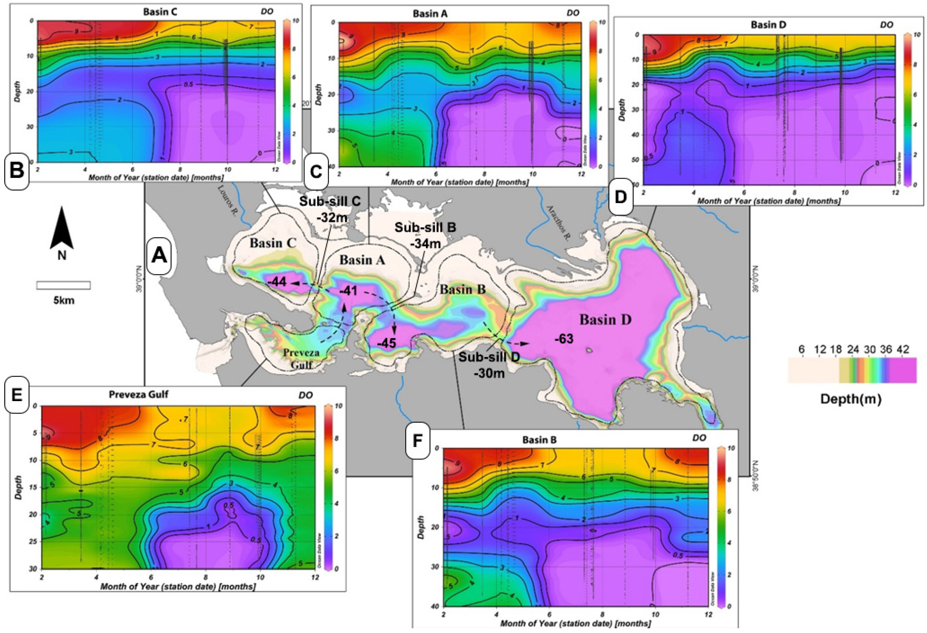
  • June to September: The summer period was characterized by the lowest density differences (less than 2 kg/m3) and the seawater intrusion was very limited, affecting mostly the sill. The water column was hypoxic below 18 m and anoxic below 22 m depth. Stratification was not very enhanced; the upper part of the water column reached up to 7 mg/L of DO and had a salinity of 30–33 PSU, and the density ranged from 20–22 kg/m3 (Figure 6G,J,M). Below a depth of 10 m, the salinity was greater than 36 PSU and homogeneously distributed, and the density was greater than 25 kg/m3. The denser water was mainly detected in Basin D (27.8 kg/m3). Hypoxia isoline presented its minimum depth at 10 and 11 m in Basins C and B, respectively (Figure 6A). It is worth noting that the DO at the seabed close to Louros River had a high value of 4 mg/L (Figure 6D). The biggest part of the gulf’s seabed was anoxic apart from Preveza Strait and part of the Preveza Gulf.
  • October to January: During the fall–winter period density difference ranged between 1.4 and 2.5 kg/m3, respectively, and ventilation of the water column happened through the mid-water at depths between 10 and 25 m. The mid-water oxygenation reached Basin B (Figure 6H). Apart from the Preveza Gulf seabed, the rest of Amvrakikos Gulf’s bottom was anoxic (Figure 6E). The 2 mg/L oxygen isoline in this period was higher at the E and SE part of the gulf as it reached a depth of 11 m and 8 m, respectively, whereas at the W part it was found at 12 m depth (Figure 6B). The seawater of salinity > 37 PSU spread at the bottom of Preveza Gulf, and it covered the mid-water of Basin A. In the rest of the gulf, the water column at depths from 15 to 25 m had a salinity of 36.5 PSU, and dropped to 36 PSU below 25 m (Figure 6K). The density at the upper part of the water column ranged from 20 to 23 kg/m3, whereas from a depth of 10 m to the bottom it varied from 24 to 27 kg/m3.
  • February to May: It was observed that during the winter–spring period, maximum oxygenation of the seabed occurred. Ventilation happened from the bottom part of the water column (20 m to the seafloor) (Figure 6I). Preveza Gulf and Basins A and B were very well oxygenated (5–8 mg/L) (Figure 6F,I). Regarding Basin D, this was the only period that it was oxygenated and became partly hypoxic (1.6 mg/L). The hypoxia interface was recorded at a minimum depth of 8 m in the east, whereas it remained under 10 m in the rest of the Gulf (Figure 6C). The water column was highly stratified and the salinity, which at the upper part presented a minimum of 24 PSU, quickly reached 36.5 PSU at 10 m depth. The salinity at the mouth of the gulf presented a maximum of 39 PSU, whereas at the bottom it had a maximum salinity of 37 PSU. Density also fluctuated from 15 kg/m3 at the top to 26–27 kg/m3 at the bottom, and it presented a maximum of 29 kg/m3 at the mouth of the gulf.
To quantify the gulf’s seafloor area and the monthly volume of the water that was hypoxic/anoxic, radar charts were constructed using the “Unit < DO” variables described in Section 2.1.2. Hence, three different radar charts were constructed describing the DO percentages (DO < 0.5 (purple color), <1 (petrol-blue color), <2 (green color), <4 (beige color) mg/L) for each unit (Vol, Vol36.2, B.area) (Figure 7a–c). The DO percentage of the gulf’s total water volume refers to both DO concentration in the brackish and the underlying saline mass contained within the gulf (Figure 7a). A total of 80% of the water volume had DO < 4 mg/L from June to August, and it was reduced to a minimum of 45% in January, when HFS and HWS occurred. Almost 40% of the total water volume was permanently hypoxic and increased up to a maximum of 60% in July. A DO < 1 mg/L percentage ranged from 30% in the winter months to 45% in summer. Almost 10% of the water volume was anoxic throughout the year and rose to 40% from August to October. During the HSI period (March–April), anoxia diminished to a minimum of 10% (Figure 7a).
To isolate the saline mass characterized by low DO concentration and observe its annual fluctuation, measurements with salinity < 36.2 PSU were excluded (as described in Section 3.1). Thus, the total volume percentage of this saline stagnant bottom mass was re-estimated using the 36.2 PSU lower threshold (Figure 7b). More than 90% of this mass had DO < 4 mg/L and 80–85% was hypoxic throughout the year. A total of 60% was characterized by DO < 1 mg/L from February to May and increased to 70% from July to January. For six months (August to February), 60% was anoxic and decreased sharply from mid-March to May, reaching a minimum percentage of 22% in April.
Regarding the DO concentrations at the gulf’s seafloor, the last value of each CTD cast was used. A total of 70% of the seafloor area had less than 4 mg/L from July to November, whereas from December to May it ranged between 55 and 65%. When the freshwater supply (HFS) and wind speed (HWS) were at their higher levels, the lowest DO < 4 mg/L percentage was recorded (Figure 7c). A total of 40% of the seabed was hypoxic throughout the year and increased to 72% from July to November. The concentration of DO < 1 mg/L ranged between 40 and 65% from mid-May to January and decreased to 25–35% from February to May, with the lowest percentage observed during April HSI. For four months (July–November), more than 50% of the gulf’s seabed was anoxic. The anoxia that covered the seafloor diminished to 30% from December to February and reached the minimum value (5%) in May, about a month later than the HSI (Figure 7c).

3.4. Weighting Natural Forcing Contribution—Factor Analysis

To detect which of the known natural drivers were correlated with the oxygenation of the gulf, factor analysis was performed (see methodology for variables) and two factors that controlled data variance through eigenvalue decomposition and Varimax rotation were determined.
Factor 1 explained the largest proportion (48.1%) of the total variance and had high positive loadings for density difference (Density Diff.), B.area > 0.5, B.area > 1, Vol > 1, Vol36.2 > 0.5, and Vol36.2 > 1 (0.83–0.99) and moderate loading for B.area > 2 (0.68) (Figure 8A). Factor 1 was interpreted as the “Density Difference” factor and provided information about the influence of horizontal density gradients between the Ionian Sea and the sill on the gulf’s oxic, hypoxic, and anoxic conditions. Interpretation of the factor loadings suggests that a high density difference was correlated with increased percentages of total and bottom mass volume and seabed coverage of low DO concentrations (>0.5 mg/L). This means that the parts of the water column and seafloor that were characterized by hypoxic–anoxic conditions were getting oxygenated. The factor score time series (Figure 8B) showed a seasonal variation of the first factor’s influence, which coincides well with the seasonal density difference shown in Figure 5A.
Factor 2 accounted for 45.4% of the total variance of the variables and showed high loadings on river supply, wind speed2, B.area > 4, Vol > 1, Vol > 2, Vol > 4, Vol36.2 > 2, and Vol36.2 > 4 (0.75–0.99) (Figure 8A). This factor was characterized as the “river supply and wind speed” factor, reflecting the influence of the two rivers’ freshwater inflow and the wind on the oxic, hypoxic, and anoxic regimes of the Gulf. The factor loading profile suggested that high freshwater supply (HFS) and high wind speed (HWS) were highly correlated with a clear increase in percentages of total seawater volume and saline bottom water masses that appeared to be better oxygenated (Vol > 1 mg/L, B.area > 2 mg/L). Moreover, HFS and HWS increased the areal coverage of seabed that was better oxygenated (>4 mg/L). Factor 2 showed high values during the winter–spring period (Figure 8B) when HFS and HWS were observed (Figure 5B,C).

3.5. Geomorphology and Site-Specific Dynamics

Site-specific oxygen depletion is compiled in Figure 9, which could be used as an integrative management guideline. Basin D, which was the most distant from the Ionian Sea and was separated by Basin B with a sub-sill of −30 m, experienced the worst situation since it was anoxic below −20 m depth throughout the year apart from February to May (Figure 9D). This period coincided with the HSI from the Ionian Sea, which was triggered by the seasonal horizontal density gradients. A high correlation between the water volume/seabed oxygenation with the density difference (Figure 8A) revealed that the seasonal density horizontal gradient was the main driver that reduced the anoxia in Basin D but also the rest of the gulf during this period. The DO of Basin D was increased only by 1 mg/L and the anoxic mass became almost hypoxic (Figure 9D).
The low correlation between the riverine inflow and anoxia reduction shows that despite the Aracthos River flowing into Basin D, enhanced stratification interrupted the freshwater from effectively diffusing deeper into the anoxic mass and permanently oxygenating it. Yet, the riverine inflow appeared to be highly correlated with the oxygenation of volume/areas with DO concentration greater than 2 and 4 mg/L. The wind also appeared to play a major role in the gulf’s oxygenation, especially during the period of stagnation (starting in June), when the hypoxia isoline retreated 5 m deeper.
Hypoxic/anoxic conditions were also observed in the remote Basin C, which was separated by the sub-sill C (−32 m), where the Louros River flows. Stratification was enhanced, especially during winter months, whereas anoxia prevailed from July to at least December, from a depth of −18 m to the seabed. Basin C’s anoxic mass was better oxygenated than Basin D and rose to a maximum of 3 mg/L of DO for almost half of the year (Figure 9B).
Basins A and B presented almost identical monthly DO fluctuation. Hypoxia/anoxia were present from June to December from a depth of about −15 m to the seafloor. During winter–spring months, when a high-density difference forced greater amounts of seawater to enter the gulf, the water column from −25 m to the seabed was well oxygenated (up to 5 mg/L). However, mid-waters (15–25 m depth) remained hypoxic all year round. Although Basin A was the closest to the Ionian Sea, it preserved anoxic conditions for at least six months (June–December), whereas it was well oxygenated for the rest of the year. Finally, in Preveza Gulf, which was the first receptor of the oxygenated Ionian seawater, hypoxic/anoxic conditions prevailed from June to October. Generally, slightly better conditions appeared in Basin A compared to B due to the shorter distance of the basin from the sill and to the presence of sub-sill B (−34 m).

4. Discussion

The sill that separates the Ionian Sea from Amvrakikos Gulf proved to be a highly dynamic and complex ecosystem; hence, it needs to be carefully examined in future coastal management plans. First, the Preveza Strait is a densely inhabited area that usually suffers from flooding events and coastal erosion. In addition, due to the hypoxic conditions that prevail along the rest of the gulf, a great part of the Ionian Sea’s and the gulf’s biomass is forced to accumulate at the sill. A geophysical survey was performed for the first time at the sill, showing that a two-layer water circulation pattern was formed at the area of the sill due to the seasonal density difference between the Ionian Sea and Amvrakikos Gulf (Figure 10A), which acts as the main natural driver that generates horizontal pressure gradients and forces the denser oxygenated seawater to intrude [14,27]. Ref. [27] supported that tide fluctuation has a negligible role in the gulf’s oxygenation. However, the tide proved to affect the horizontal water intrusion through the sill by creating tidal jets [49] that intensified the seawater intrusion velocity during high tide, whereas low tide favored the outflow of the brackish water. This was also observed at Preveza Gulf, where a timelapse of tide-triggered seawater intrusion was captured entering the gulf during high tide (Figure 3). Finally, regarding the sill, the enhanced backscatter areas that were captured in November at mid-water (Figure 4) could be correlated with enhanced mixing and turbulence between the seawater and anoxic mass but also possibly with suspended material such as planktonic assemblages that are generally favored in sills [13,50].
Apart from the tide, it was found that external forces such as wind intensity and river inflow affected the spatio-temporal distribution of DO in the gulf. Factor analysis confirmed that the main driver for the gulf’s ventilation is density difference (Figure 10A) [27]. However, diffusive and vertical mixing processes such as wind forcing and river inflow were positively correlated with the oxygenation of water volume and area above or within the pycnocline range that had DO concentrations greater than 2 mg/L, which were spatially explained as the shallower parts of the gulf. The high-intensity wind in particular was proven to decrease the water column stratification and thus decrease the hypoxic conditions [51].
Strong winds are often responsible for upwelling [52]. The three massive fish mortality events in Amvrakikos Gulf occurred in December, January, and February due to suffocation at the eastern and western parts of the gulf (Figure 1A,C). Considering the relatively shallow depth (8 m) of the hypoxia isoline (Figure 6C) during the winter–spring period and the lower stratification, the persistent E-W winds could deviate the freshwater discharge and reduce the stratification [51]. These conditions could facilitate the upwelling of hypoxia even to the surface, which is a known phenomenon called “water turnover” by local fishermen. The upward shift of the hypoxic water masses limits the deployment of the fish-farm cages (maximum cage depth: 8–12 m) and increases the risk of an accident [53]. The lack of oxygen due to this process is possibly responsible for the death of hundreds of tons of fish in Amvrakikos.
Annual quantification of the DO masses proved that the density difference is indeed the main ventilation driver since the anoxic volume was reduced to 10% during high density difference (winter–spring), from 40% in summer. The natural drivers that were examined with factor analysis were the density difference, the wind intensity, and the river inflow. However, more parameters, such as the production of organic matter, microbial activity, and other physical processes (e.g., internal tide, internal waves), may contribute to the oxygen depletion and mixing in the gulf [54,55], but they remain to be measured and tested.
Knowledge of the hypoxic conditions’ spatial variability in topographically complicated coastal areas is essential for the establishment of integrated plans for their management [56]. Hypoxia/anoxia development in Amvrakikos Gulf is not uniform but depends on the geomorphology of the basins contained within the gulf and the timing of the natural ventilation drivers. Basin D, which is located in the eastern part of the gulf, is the basin that was oxygenated the least compared to the other basins. This happened mainly due to its distance from the open sea [27], which is the main oxygen supplier, but also due to the presence of the Aracthos River, which enhances stratification. Slightly better conditions were observed at Basin C, where the Louros River is present. Furthermore, the sub-sills that separate the basins were responsible for limiting the lateral movement of the oxygenated water, making them prone to the development of hypoxic-anoxic conditions.
Hypoxia proved to be persistent throughout the year. Apart from the quantification radar plots that showed this (Figure 7), a consolidated T-S diagram was constructed using the whole database of CTD measurements from the gulf for a salinity range of 30–37 PSU (Figure 10B). In this plot, the seasonal temperature fluctuation of the gulf’s water was obvious (February: 10–18 °C, August 16–28 °C), and density fluctuated in February from 23.5 to 28 kg/m3 when the pycnocline was observed to be weaker and in August from 19–27 kg/m3 (Figure 10A). The salinity of the water with DO < 2 mg/L remained over 36.2 PSU throughout the year has and had a temperature that ranged from 15 to 23 °C. The water with these characteristics represents the stagnant bottom anoxic to hypoxic mass that lies under the brackish water (<33 PSU) in the biggest part of the gulf.
Finally, occupation of the gulf by hypoxic conditions agreed with the shrinking of the available space for the marine organisms and the decrease in the benthic invertebrates recorded by [20].

5. Conclusions

Amvrakikos Gulf is included in the growing list of hypoxic areas around the world and this project represents an attempt to monitor and understand the complex hypoxia distribution and the natural drivers that affect it under multi-spatiotemporal scales (spatial scales: sill or gulf, temporal scales: annual or diurnal). Seasonal geophysical and oceanographic surveys were performed in Amvrakikos Gulf, Greece, revealing important aspects regarding the prevailing oceanographic processes and their link to the development of hypoxic/anoxic conditions. Enriching the current knowledge in the area, the following has been concluded:
  • An almost permanent two-layered fjord estuarine circulation pattern at the sill (top brackish outflow–bottom seawater inflow) appeared to be dynamically controlled seasonally by the density differences between Amvrakikos Gulf and the Ionian Sea and daily by the tide fluctuation.
  • Natural seasonal ventilation of the gulf is mainly controlled by the density difference between the Ionian Sea and Amvrakikos Gulf, and by riverine inflows, wind, and the geomorphology of the seabed. The complex geomorphology of the gulf, with well-formed internal basins, contributes to the development and preservation of low DO conditions, especially in the eastern and larger basin D. Statistical analyses on the estimated annual variations in anoxic/hypoxic water volumes showed that the main driver that shrinks anoxia and oxygenates the gulf’s seabed is the horizontal density gradient, whereas diffusive processes and vertical mixing (e.g., riverine inflow and wind mixing) were oxygenated more effectively in the volume and bottom areas above or within the pycnocline range that had a DO concentration greater than 2 mg/L.
  • The bottom hypoxic stagnant mass expands upwards during the winter–spring period and reaches the limit of the pycnocline at a depth of at least 8 m in the east (Basin D) and 10 m in the west (Basin C) of the gulf, where the farmed fish accidents happened. This phenomenon, together with persistent strong winds (E or W) in winter, is likely to have triggered upwelling processes and bring the hypoxic mass up to the surface, leading to massive mortalities, especially in fish farms.
  • A total of 43% of the Amvrakikos Gulf seafloor is hypoxic throughout the year and during the summer–autumn period it increases up to 70%, whereas 50% of the seafloor becomes anoxic. A total of 36% of the total water volume contained in the gulf is permanently hypoxic and 10% anoxic, and increases to 62% and 40%, respectively, during the summer–autumn stagnation period. A total of 85% of the stagnant bottom saline mass that is contained within the gulf and lies under the brackish water is hypoxic throughout the year. The eastern part sustains anoxia almost the entire year, and in the rest of the Gulf for almost half of the year.
Amvrakikos Gulf is a landlocked embayment marked by an extended hypoxic/anoxic water mass. Human activities and interventions are co-responsible for the formation of a permanent dead zone, causing problems for fisheries. Despite the importance of the ecosystem for both biodiversity and local societies, little effort for monitoring and understanding the ecosystem is being made, and widely distributed urban myths exist that are mainly focused on the need for engineering interventions at Preveza Strait. This work summarizes the complexity and fragility of the ecosystem, pointing out the necessity for systematic study and in-depth evaluation before any management actions. Especially in the area of the sill, the geomorphological data and the circulation pattern should be thoroughly addressed before any interventions. Moreover, future attempts for restoration of the ecosystem (e.g., deep-water oxygenation) could be attempted based on the seasonality and spatial distribution of hypoxia, as described in this work. Future work should monitor the physical parameters and the biogeochemical processes that affect DO concentration through satellite imagery and stations to fully determine the oxygenation processes and develop a hypoxia forecast model.

Supplementary Materials

Author Contributions

Conceptualization: E.F., N.G., and C.K.; writing—original draft: N.G.; visualization: N.G.; funding acquisition: C.K., G.P., and G.F.; survey planning: C.K., G.P., D.C., E.F., N.G., and X.D.; field work: all authors; project administration: C.K.; resources: G.P. and C.K.; CTD data curation and processing: E.F., Z.G.K., and N.G.; ADCP data curation and processing: E.F. and N.G.; multibeam data curation and processing: D.C.; software: E.F. and N.G.; supervision: C.K., G.P., and E.F.; validation: E.F. and G.P.; writing—review and editing: G.P., C.K., E.F., K.-M.V., A.N., D.A. All authors have read and agreed to the published version of the manuscript.

Funding

This work was supported by the European Economic Area Financial Mechanism (EEA FM) 2009–2014 Program Area. Part of the CTD casts was provided by independent surveys of the Hellenic Centre for Marine Research (HCMR), acquired through the European Maritime and Fisheries Fund—Operational Program for Greece 2014–2020.

Acknowledgments

We would like to thank all the participants of the project, consisting of the Laboratory of Marine Geology and Physical Oceanography (LMGPO), the Laboratory of Zoology from the Department of Biology, the Department of Fisheries and Aquaculture from the University of Patras, the Hellenic Center for Marine Research (HCMR), the Department of Agricultural Technology of the Technological Education Institute of Epirus from the University of Ioannina, and the Amvrakikos Management Body. We would also like to thank the local Amvrakikos fishermen Petros Kaplanis and Ioannis Giovanos and the crew of F/R Philia for their assistance with the field sampling, the Kleopatra Marina, and Aktia Nikopolis foundation for their cooperation and supply of cartographic material. Special thanks to Kallia Spala for the successful management of the project. We wish to thank two anonymous reviewers for their corrections and for the helpful suggestions that significantly improved the quality of the manuscript.

Conflicts of Interest

The authors declare no conflict of interest.

References

  1. Barnes, R.S.K. Coastal Lagoons; CUP Archive: Cambridge, UK, 1980; Volume 1, ISBN 0521299454. [Google Scholar]
  2. Costanza, R.; D’Arge, R.; De Groot, R.; Farber, S.; Grasso, M.; Hannon, B.; Limburg, K.; Naeem, S.; O’Neill, R.V.; Paruelo, J.; et al. The value of the world’s ecosystem services and natural capital. Nature 1997, 387, 253–260. [Google Scholar] [CrossRef]
  3. Diaz, R.J.; Rosenberg, R. Spreading Dead Zones and Consequences for Marine Ecosystems. Science 2008, 321, 926–929. [Google Scholar] [CrossRef] [PubMed]
  4. Dobson, A.; Lodge, D.; Alder, J.; Cumming, G.S.; Keymer, J.; McGlade, J.; Mooney, H.; Rusak, J.A.; Sala, O.; Wolters, V.; et al. Habitat loss, trophic collapse, and the decline of ecosystem services. Ecology 2006, 87, 1915–1924. [Google Scholar] [CrossRef]
  5. Friedrich, J.; Janssen, F.; Aleynik, D.; Bange, H.W.; Boltacheva, N.; Çagatay, M.N.; Dale, A.W.; Etiope, G.; Erdem, Z.; Geraga, M.; et al. Investigating hypoxia in aquatic environments: Diverse approaches to addressing a complex phenomenon. Biogeosciences 2014, 11, 1215–1259. [Google Scholar] [CrossRef] [Green Version]
  6. Shahidul Islam, M.; Tanaka, M. Impacts of pollution on coastal and marine ecosystems including coastal and marine fisheries and approach for management: A review and synthesis. Mar. Pollut. Bull. 2004, 48, 624–649. [Google Scholar] [CrossRef] [PubMed]
  7. Libralato, S.; Caccin, A.; Pranovi, F. Modeling species invasions using thermal and trophic niche dynamics under climate change. Front. Mar. Sci. 2015, 2, 29. [Google Scholar] [CrossRef] [Green Version]
  8. Díaz, R.J.; Rosenberg, R. Introduction to Environmental and Economic Consequences of Hypoxia. Int. J. Water Resour. Dev. 2011, 27, 71–82. [Google Scholar] [CrossRef]
  9. Halpern, B.S.; Longo, C.; Hardy, D.; McLeod, K.L.; Samhouri, J.F.; Katona, S.K.; Kleisner, K.; Lester, S.E.; O’Leary, J.; Ranelletti, M.; et al. An index to assess the health and benefits of the global ocean. Nature 2012, 488, 615–620. [Google Scholar] [CrossRef] [Green Version]
  10. Hardy, J.T. Climate Change Causes, Effects, and Solutions; John Wiley Sons Ltd.: Chichester, UK, 2003; Volume 26, pp. 139–140. [Google Scholar] [CrossRef]
  11. Hu, S.; Sprintall, J.; Guan, C.; McPhaden, M.J.; Wang, F.; Hu, D.; Cai, W. Deep-reaching acceleration of global mean ocean circulation over the past two decades. Sci. Adv. 2020, 6, eaax7727. [Google Scholar] [CrossRef] [Green Version]
  12. Koutsodendris, A.; Brauer, A.; Zacharias, I.; Putyrskaya, V.; Klemt, E.; Sangiorgi, F.; Pross, J. Ecosystem response to human- and climate-induced environmental stress on an anoxic coastal lagoon (Etoliko, Greece) since 1930 AD. J. Paleolimnol. 2015, 53, 255–270. [Google Scholar] [CrossRef]
  13. Pérez-Santos, I.; Castro, L.; Ross, L.; Niklitschek, E.; Mayorga, N.; Cubillos, L.; Gutierrez, M.; Escalona, E.; Castillo, M.; Alegría, N.; et al. Turbulence and hypoxia contribute to dense biological scattering layers in a Patagonian fjord system. Ocean Sci. 2018, 14, 1185–1206. [Google Scholar] [CrossRef] [Green Version]
  14. Ferentinos, G.; Papatheodorou, G.; Geraga, M.; Iatrou, M.; Fakiris, E.; Christodoulou, D.; Dimitriou, E.; Koutsikopoulos, C. Fjord water circulation patterns and dysoxic/anoxic conditions in a Mediterranean semi-enclosed embayment in the Amvrakikos Gulf, Greece. Estuar. Coast. Shelf Sci. 2010, 88, 473–481. [Google Scholar] [CrossRef]
  15. Albanis, T.A.; Danis, T.G.; Hela, D.G. Transportation of pesticides in estuaries of Louros and Arachthos rivers (Amvrakikos Gulf, N.W. Greece). Sci. Total Environ. 1995, 171, 85–93. [Google Scholar] [CrossRef]
  16. Avramidis, P.; Iliopoulos, G.; Panagiotaras, D.; Papoulis, D.; Lambropoulou, P.; Kontopoulos, N.; Siavalas, G.; Christanis, K. Tracking Mid- to Late Holocene depositional environments by applying sedimentological, palaeontological and geochemical proxies, Amvrakikos coastal lagoon sediments, Western Greece, Mediterranean Sea. Quat. Int. 2014, 332, 19–36. [Google Scholar] [CrossRef]
  17. Tsirogiannis, I.L.; Karras, G.; Tsolis, D.; Barelos, D. Irrigation and Drainage Scheme of the Plain of Arta—Effects on the Rural Landscape and the Wetlands of Amvrakikos’ Natura Area. Agric. Agric. Sci. Procedia 2015, 4, 20–28. [Google Scholar] [CrossRef] [Green Version]
  18. Kormas, K.A.; Nicolaidou, A.; Reizopoulou, S. Temporal variations of nutrients, chlorophyll a and particulate matter in three coastal lagoons of Amvrakikos Gulf (Ionian Sea, Greece). Mar. Ecol. 2001, 22, 201–213. [Google Scholar] [CrossRef]
  19. Kotti, M.E.; Vlessidis, A.G.; Thanasoulias, N.C.; Evmiridis, N.P. Assessment of River Water Quality in Northwestern Greece. Water Resour. Manag. 2005, 19, 77–94. [Google Scholar] [CrossRef]
  20. Piroddi, C.; Moutopoulos, D.K.; Gonzalvo, J.; Libralato, S. Ecosystem health of a Mediterranean semi-enclosed embayment (Amvrakikos Gulf, Greece): Assessing changes using a modeling approach. Cont. Shelf Res. 2016, 121, 61–73. [Google Scholar] [CrossRef]
  21. Kountoura, K.; Zacharias, I. Temporal and spatial distribution of hypoxic/seasonal anoxic zone in Amvrakikos Gulf, Western Greece. Estuar. Coast. Shelf Sci. 2011, 94, 123–128. [Google Scholar] [CrossRef]
  22. Anastasakis, G.; Piper, D.J.W.; Tziavos, C. Sedimentological response to neotectonics and sea-level change in a delta-fed, complex graben: Gulf of Amvrakikos, western Greece. Mar. Geol. 2007, 236, 27–44. [Google Scholar] [CrossRef]
  23. Poulos, S.E.; Kapsimalis, V.; Tziavos, C.; Paramana, T. Origin and distribution of surface sediments and human impacts on recent sedimentary processes. The case of the Amvrakikos Gulf (NE Ionian Sea). Cont. Shelf Res. 2008, 28, 2736–2745. [Google Scholar] [CrossRef]
  24. Kapsimalis, V.; Pavlakis, P.; Poulos, S.E.; Alexandri, S.; Tziavos, C.; Sioulas, A.; Filippas, D.; Lykousis, V. Internal structure and evolution of the Late Quaternary sequence in a shallow embayment: The Amvrakikos Gulf, NW Greece. Mar. Geol. 2005, 222–223, 399–418. [Google Scholar] [CrossRef]
  25. Georgiou, N.; Fakiris, E.; Christodoulou, D.; Dimas, X.; Koutsikopoulos, C.; Papatheodorou, G. Anthropogenic impacts on the geomorphological regime of Preveza straits (Amvrakikos Gulf). In Proceedings of the 1st International Scientific Conference on Design and Management of Harbor, Coastal and Offshore Works, Athens, Greece, 8–11 May 2019. [Google Scholar]
  26. Piper, D.J.W.; Panagos, A.G.; Kontopoulos, N. Some observations on surficial sediments and physical oceanography of the Gulf of Amvrakia. Thalassographica 1982, 55, 283–294. [Google Scholar] [CrossRef]
  27. Kountoura, K.; Zacharias, I. Annual hypoxia dynamics in a semi-enclosed Mediterranean gulf. J. Mar. Syst. 2014, 139, 320–331. [Google Scholar] [CrossRef]
  28. Balistrieri, L.S.; Murray, J.W.; Paul, B. The geochemical cycling of trace elements in a biogenic meromictic lake. Geochim. Cosmochim. Acta 1994, 58, 3993–4008. [Google Scholar] [CrossRef]
  29. Lewis, B.L.; Landing, W.M. The biogeochemistry of manganese and iron in the Black Sea. Deep Sea Res. Part A Oceanogr. Res. Pap. 1991, 38, S773–S803. [Google Scholar] [CrossRef]
  30. Papatheodorou, G.; Hasiotis, T.; Ferentinos, G. Gas-charged sediments in the Aegean and Ionian Seas, Greece. Mar. Geol. 1993, 112, 171–184. [Google Scholar] [CrossRef]
  31. Kordella, S.; Christodoulou, D.; Fakiris, E.; Geraga, M.; Kokkalas, S.; Marinaro, G.; Iatrou, M.; Ferentinos, G.; Papatheodorou, G. Gas seepage-induced features in the hypoxic/anoxic, shallow, marine environment of amfilochia bay, amvrakikos gulf (Western Greece). Geosciences 2021, 11, 27. [Google Scholar] [CrossRef]
  32. Garcia-Tigreros, F.; Leonte, M.; Ruppel, C.D.; Ruiz-Angulo, A.; Joung, D.; Young, B.; Kessler, J.D. Estimating the impact of seep methane oxidation on ocean pH and dissolved inorganic radiocarbon along the U.S. mid-Atlantic Bight. J. Geophys. Res. Biogeosciences 2021, 126, e2019JG005621. [Google Scholar] [CrossRef]
  33. Friligos, N.; Balopoulos, E.T.; Psyllidou-Giouranovits, R. Eutrophication and hydrography in the Amvrakikos Gulf Ionian Sea. Fresenius Environ. Bull. 1997, 3, 71–84. [Google Scholar] [CrossRef]
  34. Arai, R.; Nakatani, N.; Okuno, T. Measurement Method of Turbidity Depth Profiles using ADCP for Monitoring of Coastal Sea Area. In Proceedings of the OCEANS 2008—MTS/IEEE Kobe Techno-Ocean, Kobe, Japan, 8–11 April 2008; pp. 1–6. [Google Scholar] [CrossRef]
  35. Merckelbach, L.M.; Ridderinkhof, H. 2. Measurements of suspended sediment concentrations from ADCP backscatter in strong currents. In Aspects of Coastal Research in Contribution to LOICZ in The Netherlands and Flanders (2002–2010); Helmholtz-Zentrum Geesthacht: Geesthacht, Germany, 2011; Volume 53. [Google Scholar]
  36. Voutsinou-Taliadouri, F.; Balopoulos, E.T.H. Geochemical and physical oceanographic aspects of the Amvrakikos Gulf (Ionian Sea, Greece). Toxicol. Environ. Chem. 1991, 31, 177–185. [Google Scholar] [CrossRef]
  37. Weiss, R.F. Helium Isotope Effect in Solution in Water and Seawater. Science 1970, 168, 247–248. [Google Scholar] [CrossRef] [PubMed]
  38. Garcia, H.E.; Gordon, L.I. Oxygen solubility in seawater: Better fitting equations. Limnol. Oceanogr. 1992, 37, 1307–1312. [Google Scholar] [CrossRef]
  39. Schlitzer, R. Ocean Data View (odv.awi.de). 2003, pp. 1–10. Available online: https://odv.awi.de/ (accessed on 1 June 2021).
  40. Parsons, D.R.; Jackson, P.R.; Czuba, J.A.; Engel, F.L.; Rhoads, B.L.; Oberg, K.A.; Best, J.L.; Mueller, D.S.; Johnson, K.K.; Riley, J.D. Velocity Mapping Toolbox (VMT): A processing and visualization suite for moving-vessel ADCP measurements. Earth Surf. Process. Landf. 2013, 38, 1244–1260. [Google Scholar] [CrossRef]
  41. Papatheodorou, G.; Demopoulou, G.; Lambrakis, N. A long-term study of temporal hydrochemical data in a shallow lake using multivariate statistical techniques. Ecol. Modell. 2006, 193, 759–776. [Google Scholar] [CrossRef]
  42. Papatheodorou, G.; Lambrakis, N.; Panagopoulos, G. Application of multivariate statistical procedures to the hydrochemical study of a coastal aquifer: An example from Crete, Greece. Hydrol. Process. 2007, 21, 1482–1495. [Google Scholar] [CrossRef]
  43. Fakiris, E.; Blondel, P.; Papatheodorou, G.; Christodoulou, D.; Dimas, X.; Georgiou, N.; Kordella, S.; Dimitriadis, C.; Rzhanov, Y.; Geraga, M.; et al. Multi-frequency, multi-sonar mapping of shallow habitats-efficacy and management implications in the National Marine Park of Zakynthos, Greece. Remote Sens. 2019, 11, 461. [Google Scholar] [CrossRef] [Green Version]
  44. Fakiris, E.; Zoura, D.; Ramfos, A.; Spinos, E.; Georgiou, N.; Ferentinos, G.; Papatheodorou, G. Object-based classification of sub-bottom profiling data for benthic habitat mapping. Comparison with sidescan and RoxAnn in a Greek shallow-water habitat. Estuar. Coast. Shelf Sci. 2018, 208, 219–234. [Google Scholar] [CrossRef]
  45. Asahi, H.; Takahashi, K. A new insight into oceanography with multivariate and time-series analyses on the 1990–1999 planktonic foraminiferal fluxes in the Bering Sea and the central subarctic Pacific. Mem. Fac. Sci. Kyushu Univ. Ser. D Earth Planet. Sci. 2008, 32, 73–96. [Google Scholar] [CrossRef]
  46. Johnson, G.W.; Ehrlich, R.; Full, W.; Ramos, S. Chapter 18—Principal Components Analysis and Receptor Models in Environmental Forensics. In Introduction to Environmental Forensics, 3rd ed.; Murphy, B.L., Morrison, R.D., Eds.; Academic Press: San Diego, CA, USA, 2015; pp. 609–653. ISBN 978-0-12-404696-2. [Google Scholar] [CrossRef]
  47. Stigebrandt, A. Hydrodynamics and Circulation of Fjords BT—Encyclopedia of Lakes and Reservoirs; Bengtsson, L., Herschy, R.W., Fairbridge, R.W., Eds.; Springer: Dordrecht, The Netherlands, 2012; pp. 327–344. ISBN 978-1-4020-4410-6. [Google Scholar] [CrossRef]
  48. Bagiorgas, H.S.; Assimakopoulos, M.N.; Theoharopoulos, D.; Matthopoulos, D.; Mihalakakou, G.K. Electricity generation using wind energy conversion systems in the area of Western Greece. Energy Convers. Manag. 2007, 48, 1640–1655. [Google Scholar] [CrossRef]
  49. Stigebrandt, A.; Aure, J. Vertical Mixing in Basin Waters of Fjords. J. Phys. Oceanogr. 1989, 19, 917–926. [Google Scholar] [CrossRef] [Green Version]
  50. Kim, Y.H.; Voulgaris, G. Estimation of Supsended Sediment Concentration in Estuarine Environmetns Using Acoustic Backscatter from an ADCP. In Proceedings of the International Conference on Coastal Sediments, Clearwater Beach, FL, USA, 18–23 May 2003; pp. 1–10. [Google Scholar]
  51. Liuqian, Y.; Fennel, K.; Arnaud, L. A modeling study of physical controls on hypoxia generationin the northern Gulf of Mexico. J. Geophys. Res. Ocean. 2015, 120, 2813–2825. [Google Scholar] [CrossRef]
  52. Feng, Y.; Fennel, K.; Jackson, G.A.; Dimarco, S.F.; Hetland, R.D. A model study of the response of hypoxia to upwelling-favorable wind on the northern Gulf of Mexico shelf. J. Mar. Syst. 2014, 131, 63–73. [Google Scholar] [CrossRef] [Green Version]
  53. Ram, A.; Jaiswar, J.R.M.; Rokade, M.A.; Bharti, S.; Vishwasrao, C.; Majithiya, D. Nutrients, hypoxia and Mass Fishkill events in Tapi Estuary, India. Estuar. Coast. Shelf Sci. 2014, 148, 48–58. [Google Scholar] [CrossRef]
  54. Conley, D.J.; Bjorck, S.; Bonsdorff, E.; Carstensen, J.; Destouni, G.; Gustafsson, B.O.G.; Hietanen, S.; Kortekaas, M.; Kuosa, H.; Meier, H.E.M.; et al. Critical Review Hypoxia-Related Processes in the Baltic Sea. Environ. Sci. Technol. 2009, 43, 3412–3420. [Google Scholar] [CrossRef] [Green Version]
  55. Peña, M.A.; Katsev, S.; Oguz, T.; Gilbert, D. Modeling dissolved oxygen dynamics and hypoxia. Biogeosciences 2010, 7, 933–957. [Google Scholar] [CrossRef] [Green Version]
  56. Virtanen, E.A.; Norkko, A.; Nyström Sandman, A.; Viitasalo, M. Identifying areas prone to coastal hypoxia—The role of topography. Biogeosciences 2019, 16, 3183–3195. [Google Scholar] [CrossRef] [Green Version]
Figure 1. (A) General bathymetry of Amvrakikos Gulf, locations of massive farmed-fish mortality events (black stars), and CTD stations involved in this work (yellow triangle CTD stations from the Hellenic Center for Marine Research and blue circles from the Laboratory of Marine Geology & Physical Oceanography), and the location of the profile of Figure 6, (B) Geophysical survey track lines of the current study, (C) fish mortality event in February 2008, (D) detailed bathymetry of the sill acquired during this study using MBES, indicated in Figure 1E and Figure 2 with a black rectangle, and (E) magnified 3D bathymetry of the Preveza Strait showing the navigation channel, subsea tunnel, dredged west plateau, and scour holes.
Geosciences 11 00241 g001
Figure 2. Τwo-layer circulation pattern distinguished in three different levels: (A) 0–7 m, (B) 7–12 m, and (C) 12-bottom; (D) cross-section showing the flow direction perpendicular to the straits as indicated in map 2 h; (E) flow direction cross-section perpendicular to the straits as indicated in map 2 h; (F) flow direction cross-section perpendicular to the straits as indicated in map 2 h; (G) ADCP profile parallel to the Preveza Strait showing the brackish mass outflowing to the SSW on the top part of the water column and the seawater flowing into the gulf; and (H) a map showing the location of d, e, f, and g (sections presented in this figure were made using the VMT software [38]).
Geosciences 11 00241 g002
Figure 3. (A) ADCP data (blue dots) in April at the sill and section location (red polygon- averaged values of ADCP data), (BD) SW-NE sections describing the tidal intrusion as monitored by the ADCP showing the eastern velocity (cm/s) during different time steps based on the tide fluctuation, and (EG) relative backscatter intensity sections.
Geosciences 11 00241 g003
Figure 4. (AC) CTD-1,-2 profiles (dissolved oxygen, salinity, temperature) at Preveza Gulf in November, (D) ADCP section showing the eastern velocity and the two selected CTD profile locations, (E) backscatter intensity section of the water column, (F) vertical velocity section, and (G) bottom eastern velocity (cm/s), CTD-1,-2 acquired during the November 2016 survey, and bottom collision zone between the inflowing seawater with the outflowing anoxic mass.
Geosciences 11 00241 g004
Figure 5. (A) Density difference (kg/m3) per month between the Ionian Sea and the sill, HSI: high seawater intrusion; (B) freshwater supply per month in m3/s from Aracthos (light orange) and Louros (orange) rivers, HFS: high freshwater supply (data acquired by Hellenic Public Power Corporation—HPPC, DEI); and (C) monthly mean wind speed (m/s) chart of Amvrakikos Gulf (Hellenic National Meteorological Service—HNMS).
Geosciences 11 00241 g005
Figure 6. (AC) seasonal fluctuation of the hypoxia isoline (DO:2 mg/L) depth seasonally, (DF) seasonal DO concentration in mg/L at the bottom of the gulf, (GI) longitudinal sections of the gulf showing the seasonal DO distribution, (JL) longitudinal sections of the gulf showing the salinity distribution, and (MO) longitudinal sections of the gulf showing the salinity distribution.
Geosciences 11 00241 g006
Figure 7. Radar plots showing (A) total water volume percentage based on different DO classes (DO < 4 mg/L, DO < 2 mg/L, DO < 1 mg/L, DO < 0.5 mg/L), (HFS: high freshwater supply), (HSI: high seawater intrusion), (HWS: high wind speed); (B) water volume percentage of CTD with salinity higher than 36.2 PSU based on different DO; and (C) seafloor area percentage that is covered by different DO range classes monthly.
Geosciences 11 00241 g007
Figure 8. (A) FA table showing the factor loadings (yellow box: communalities and black box: total variance explained, natural ventilation drivers in bold: density difference, river supply, wind speed2), (B) monthly Factor 1 (F1) and Factor 2 (F2) scores (related to density difference oxygenation mechanism and riverine inflow–wind mixing). Factor scores are normalized to the 0–1 range for better visualization in the radar plots.
Geosciences 11 00241 g008
Figure 9. Bathymetry of Amvrakikos Gulf and Basins A, B, C, D locations (A), and DO distribution throughout the year in Basin C (B), Basin A (C), Basin D (D), Preveza Gulf (E), and Basin B (F).
Geosciences 11 00241 g009
Figure 10. (A) Density difference between the Ionian Sea and sill (red line, left axis), (B) density difference between the Ionian Sea and the deep water of Basin D.
Geosciences 11 00241 g010
Table 1. Oceanographic parameters of the top brackish and bottom saline water of Amvrakikos Gulf during different seasons (compiled from the literature).
LayerParameters (Unit)WinterSummerReference
Top
(Brackish)
Salinity (PSU)11–2231–33[27]
Temperature (°C)12–1423.5–27/29[26,27]
Dissolved oxygen (mg/L)7.5–9[14]
PH8[14]
Bottom
(Saline)
Salinity (PSU)38–3936–37[27]
Temperature (°C)15–16[26]
Dissolved oxygen (mg/L)2–6≤2[14]
PH7.6[14]
Publisher’s Note: MDPI stays neutral with regard to jurisdictional claims in published maps and institutional affiliations.

