
MATLAB Virtual Toolbox for Retrospective Rockfall Source Detection and Volume Estimation Using 3D Point Clouds: A Case Study of a Subalpine Molasse Cliff


Abstract
1. Introduction
2. Toolbox for 3D Point Cloud Processing
3. Toolbox-Specific Landslide Package: Retrospective Rockfall Source Detection and Volume Estimation Processing
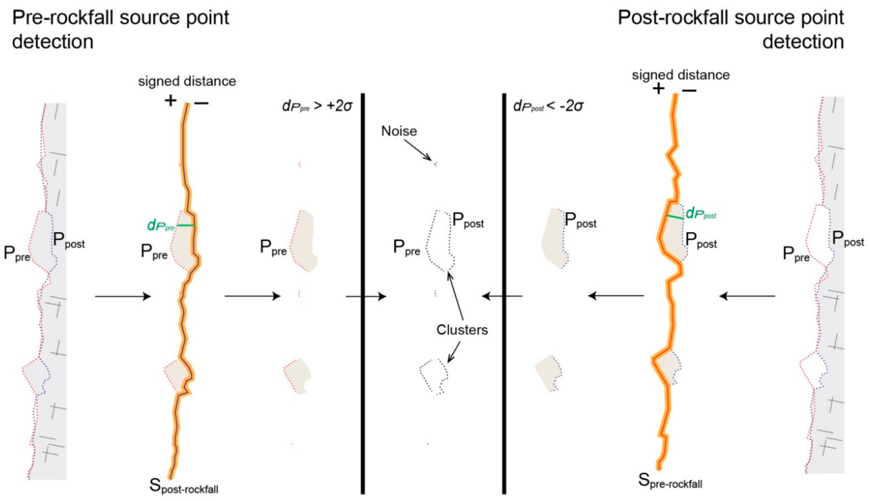
3.1. Step 1: Rockfall Source Location Extract by Thresholding
- Points belonging to topographic changes assumed to result from rockfalls.
- Points belonging to unchanged topography assumed to be stable surfaces.
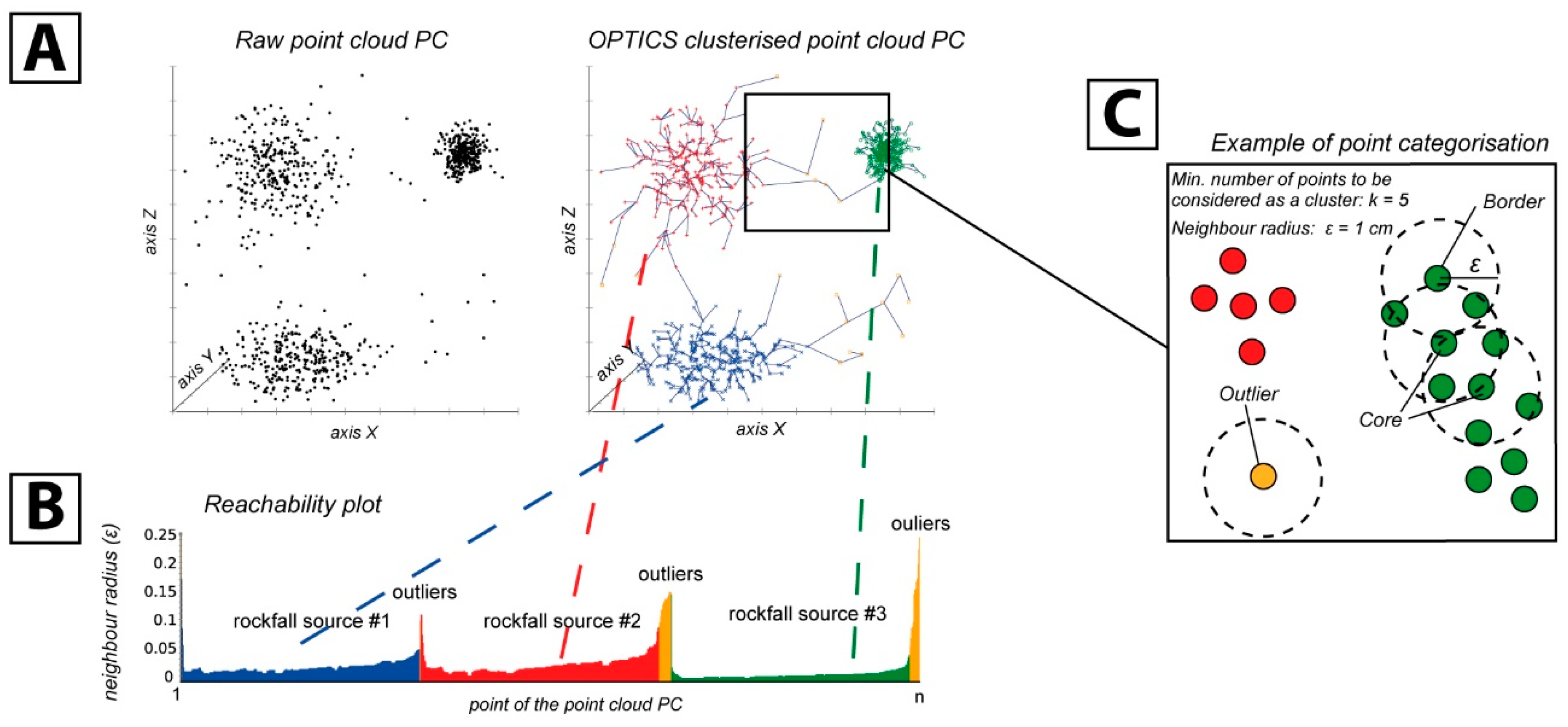
3.2. Step 2: Clustering Rockfall Sources
- A core point, if the neighborhood of radius (ε), has at least k-points (reachable points);
- A border point possesses at least one core point within a radius (ε);
- An outlier is a point with no point or no core point within its radius (ε).
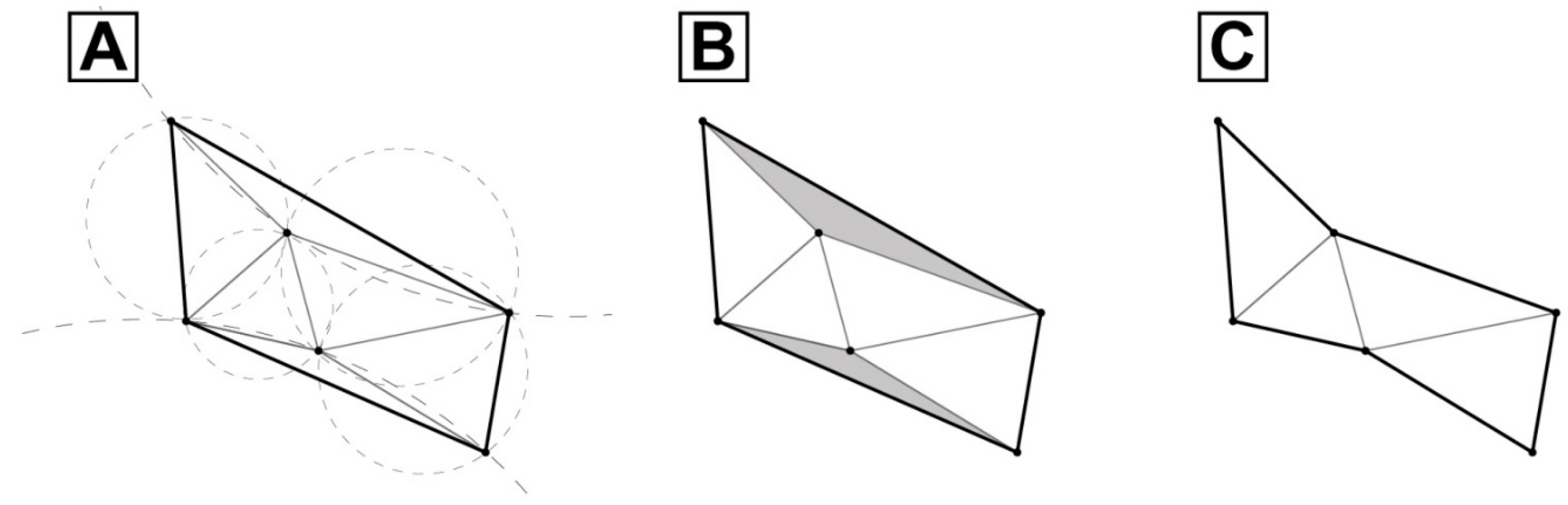
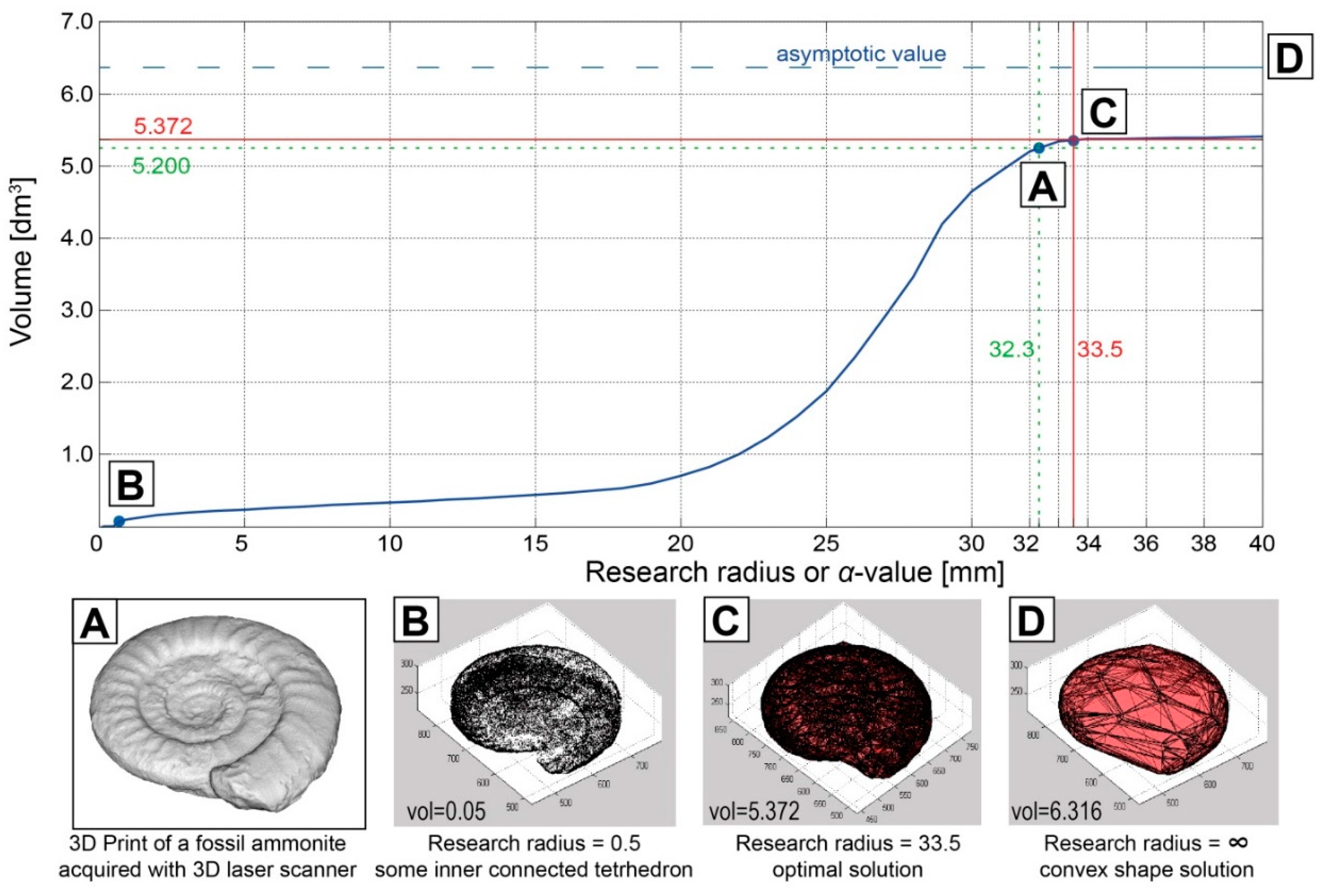
3.3. Step 3: Rockfall Source Volume Estimation
- If α = ∞, Sα is the convex hull of the point cloud;
- If α = 0, Sα is each point of the point cloud itself;
- If 0 < α < ∞, Sα will be the largest polyhedron or shape connecting m points of the point cloud.
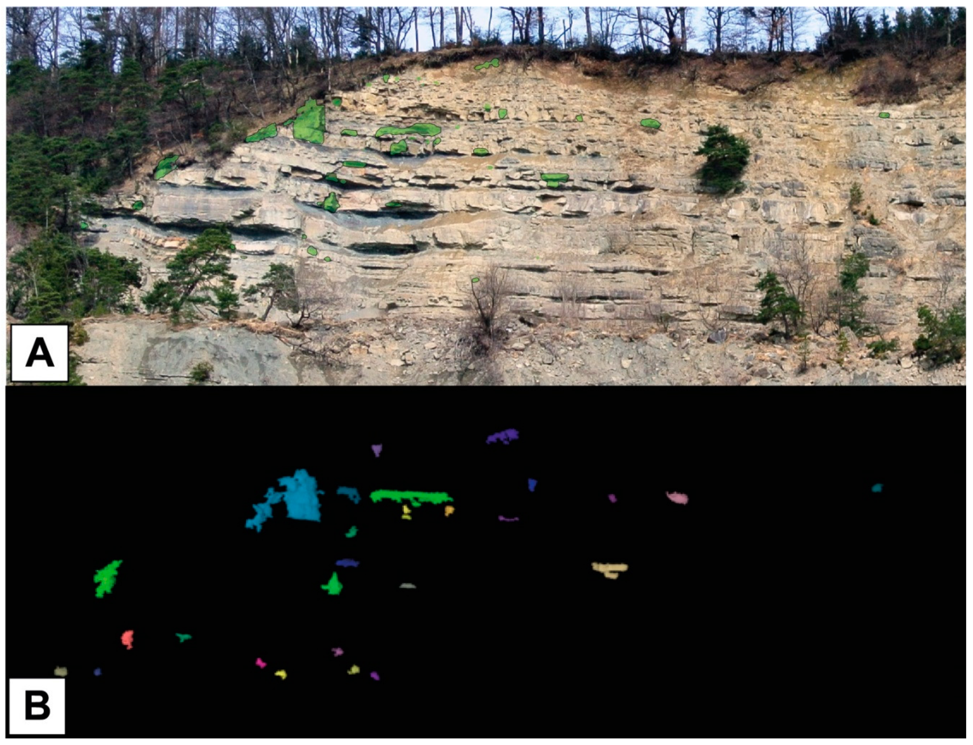
4. Case Study
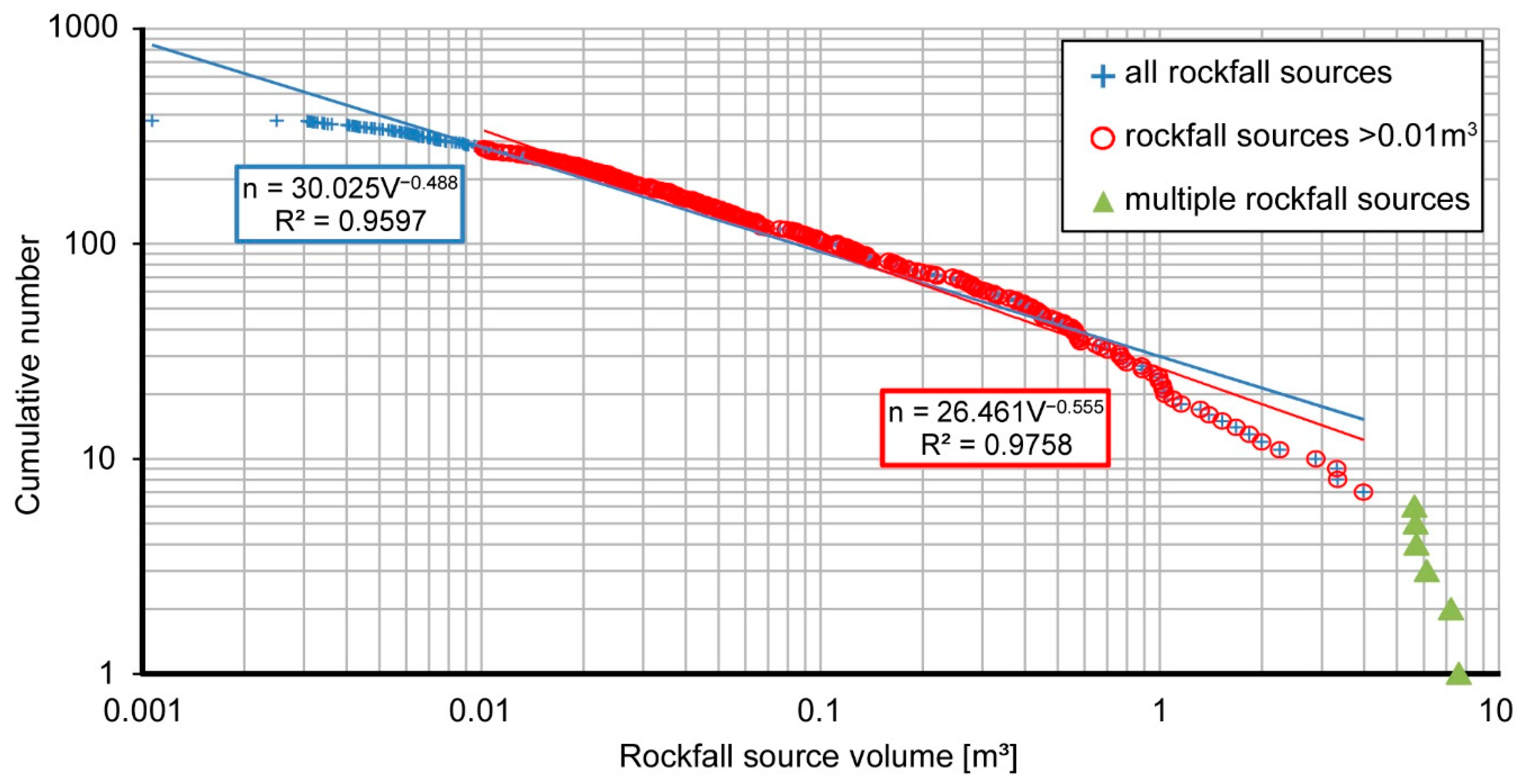
5. Results
6. Discussion
7. Conclusions
Supplementary Materials
Author Contributions
Funding
Institutional Review Board Statement
Informed Consent Statement
Acknowledgments
Conflicts of Interest
Appendix A


| RockfallQuantification Functions | |
|---|---|
| Step 1: RockfallExtract | Extract point belonging to surface change from two PointCloud objects |
| Step 2: RockfallSegment | Individualize single rockfall event by clustering index on PointCloud |
| dbscan_optics | Density-Based Spatial Clustering of Applications with Noise [42] and OPTICS improvement [43] |
| dist | Compute Euclidean distance between points in the cloud |
| epsilon | Compute optimal epsilon radius according to gamma function approximation (Daszykowski et al., 2002) |
| Step 3: RockfallVolume | Compute volume and center of mass of PointCloud |
| trueboundary | Find boundary points to define shape of PointCloud |
| volumes_tetra | Compute volume of single tetrahedron |
| alphavol | Compute α-concave hull from PointCloud [45] |
| MATLAB Classes—Key Terms | |
|---|---|
| Class definition | Description of what is common to every instance of a class |
| Classes | A class describes a set of objects with common characteristics |
| Super classes | Classes that are used as a basis for the creation of more specifically defined classes (i.e., subclasses) |
| Subclasses | Classes that are derived from other classes and that inherit the methods, properties, and events from those classes (subclasses facilitate the reuse of code defined in the superclass from which they are derived) |
| Objects | Specific instances of a class, which contain actual data values stored in the object’s properties |
| Properties | Data storage for class instances |
| Methods | Special functions that implement operations that are usually performed only on instances of the class |
| Packages | Folders that define a scope for a class and function naming |
| PointCloud Methods | |
|---|---|
| Add | Add the content of a given point cloud to this one |
| addNoise | Add simulated noise to the true point positions with following possibility: Gaussian position smearing Outliers to simulate completely wrong position Drop out some points by replacing points position by NaNs |
| ComputeBoundaries | Compute the Boundary points |
| ComputeCurvature | Compute the curvatures at each point using: Estimation of the curvature based on [64] Variation of the surface from correlation of point clouds based on [65] |
| ComputeDelaunayTriangulation | Compute a 3D Delaunay triangulation using built-in MATLAB® function |
| ComputeKDTree | Compute a Kd search tree using built-in MATLAB® function |
| ComputeNormals | Compute the least squares normal vector estimation of the points based on [64] |
| ComputeOptimalNormals | Compute the adaptive normals based on neighbor size, point density, and research radius based on [66] in order to reduce normals dispersion |
| ComputeTrueDistance | Compute the mean and root mean squared distances between a PointCloud positions and a given PointCloud true positions |
| CopyTrue2MeasPos | Copy the “true” positions to the “measured” ones |
| GetMissingPropFromPC | Complete properties of an object PointCloud by getting the missing ones from other PointCloud object |
| HasTrueP | Return true if the object PointCloud has true positions |
| ImportDataFromASCII | Import data from an ASCII file |
| IsEmpty | Is the object PointCloud object empty? |
| MeshPointCloud | Create a MeshPointCloud from this PointCloud |
| MoveToCM | Move to the center of mass of another given object PointCloud |
| NormalsOutTopo | For each point, compute the sign of the normal vector to be oriented toward its indexed sensor using TLSAttribute to have normals orientation to be out of the topography |
| Plot3 | Plot the 3D coordinates of each point of the object PointCloud Positions |
| PlotCurvature | Plot the computed curvatures |
| PlotNormals | Plot the computed normals |
| PlotPCLViewer | Plot for large point cloud positions with colors or intensities using Point Cloud Library Viewer [19] |
| PlotPositionsWithColors | Plot the point cloud with the colors |
| PlotPositionsWithIntensities | Plot the point cloud with the intensities |
| RemoveNans | Remove any NaNs values in P and TrueP |
| SaveInASCII | Save object PointCloud in ASCII format |
| SaveInPCD | Save object PointCloud in PCD format for open Point Cloud Library [19] |
| Size | What is the dimension of the object PointCloud? |
| Transform | Transform the object PointCloud |
| WhatColor | Query: what is the RGB color of the closest point? |
| WhatIntensity | Query: what is the intensity of the closest point? |
| MainLibrary | |
|---|---|
| PointCloud | Constructor of the object PointCloud and related methods |
| AffinTransform | Apply an affine transformation to object PointCloud |
| AlphaBoundary | Determine the convex hull of the object PointCloud using [45] |
| EuclDist | Compute the Euclidean distance between two vectors of 3D points. |
| HalfWayPoints | Loop on all the possible pairs in the input points and compute the halfway point |
| ImportPointCloudFromASCII | Create a PointCloud object from a given input data (in ASCII format), allowing the user selection of the specific point cloud properties |
| MeshPointCloud | Class to hold mesh grids as created by functions like GridFit |
| PlaneMesh | Create a synthetic planar grid of points |
| Plot3DPointClouds | Display one object PointCloud with defined property |
| PlotMultiPointClouds | Display several objects PointCloud with defined property |
| Quat2Rot | Convert (unit) quaternion representations to (orthogonal) rotation matrices R |
| RemoveDuplicate3DPoints | Remove the duplicates in a set of 3D points |
| Rot2Quat | Converts (orthogonal) rotation matrices R to (unit) quaternion representations |
| RotationMatrix | Compute the rotation matrix given the Eulerian rotation angles |
| SubSampling | Create a sub sample of a given object PointCloud |
| TransformMatrix | Given the rotation angles and a translation vector, provides a transformation matrix |
| TriangularMesh | Decompose a given triangle form mesh into smaller triangles |
| Vector | A class to efficiently store any other property or type of data |
| PointCloudComparison | |
|---|---|
| ComparePoint2Point | Compute comparison using the shortest point to point distance. Calculation is made using Euclidean distance between a given point in PointCloud A to the closest point in PointCloud B with output as absolute differences. |
| ComparePoint2Surface | Compute comparison using the shortest point to surface distance. Calculation is made between a given point in PointCloud A and the distance parallel to the normal to the closest point in PointCloud B with output as signed differences. |
References
- Buckley, S.J.; Enge, H.D.; Carlsson, C.; Howell, J.A. Terrestrial laser scanning for use in virtual outcrop geology. Photogramm. Rec. 2010, 25, 225–239. [Google Scholar] [CrossRef]
- Matasci, B.; Carrea, D.; Abellan, A.; Derron, M.-H.; Humair, F.; Jaboyedoff, M.; Metzger, R. Geological mapping and fold modeling using Terrestrial Laser Scanning point clouds: Application to the Dents-du-Midi limestone massif (Switzerland). Eur. J. Remote Sens. 2015, 48, 569–591. [Google Scholar] [CrossRef]
- Milan, D.J.; Heritage, G.L.; Hetherington, D. Application of a 3D laser scanner in the assessment of erosion and deposition volumes and channel change in a proglacial river. Earth Surf. Process. Landf. 2007, 32, 1657–1674. [Google Scholar] [CrossRef]
- Micheletti, N.; Tonini, M.; Lane, S.N. Geomorphological activity at a rock glacier front detected with a 3D density-based clustering algorithm. Geomorphology 2017, 278, 287–297. [Google Scholar] [CrossRef]
- Jaboyedoff, M.; Oppikofer, T.; Abellán, A.; Derron, M.-H.; Loye, A.; Metzger, R.; Pedrazzini, A. Use of LIDAR in landslide investigations: A review. Nat. Hazards 2012, 61, 5–28. [Google Scholar] [CrossRef]
- Slob, S.; Hack, R. 3D Terrestrial Laser Scanning as a New Field Measurement and Monitoring Technique. In Engineering Geology for Infrastructure Planning in Europe; Lecture Notes in Earth Sciences; Hack, R., Azzam, R., Charlier, R., Eds.; Springer: Berlin/Heidelberg, Germany, 2004; Volume 104, pp. 179–189. [Google Scholar]
- Sturzenegger, M.; Stead, D. Quantifying discontinuity orientation and persistence on high mountain rock slopes and large landslides using terrestrial remote sensing techniques. Nat. Hazards Earth Syst. Sci. 2009, 9, 267–287. [Google Scholar] [CrossRef]
- Lucieer, A.; Jong, S.M.d.; Turner, D. Mapping landslide displacements using Structure from Motion (SfM) and image correlation of multi-temporal UAV photography. Prog. Phys. Geogr. 2014, 38, 97–116. [Google Scholar] [CrossRef]
- Stumpf, A.; Malet, J.-P.; Allemand, P.; Pierrot-Deseilligny, M.; Skupinski, G. Ground-based multi-view photogrammetry for the monitoring of landslide deformation and erosion. Geomorphology 2014, 231, 130–145. [Google Scholar] [CrossRef]
- Roncella, R.; Forlani, G. A Fixed Terrestrial Photogrammetric System for Landslide Monitoring. In Modern Technologies for Landslide Monitoring and Prediction; Springer Natural Hazards; Scaioni, M., Ed.; Springer: Berlin/Heidelberg, Germany, 2015; pp. 43–67. [Google Scholar]
- Voumard, J.; Derron, M.-H.; Jaboyedoff, M.; Bornemann, P.; Malet, J.-P. Pros and Cons of Structure for Motion Embarked on a Vehicle to Survey Slopes along Transportation Lines Using 3D Georeferenced and Coloured Point Clouds. Remote Sens. 2018, 10, 1732. [Google Scholar] [CrossRef]
- Rosser, N.; Petley, D. Monitoring and modeling of slope movement on rock cliffs prior to failure. In Landslides and Engineered Slopes. From the Past to the Future; Chen, Z., Zhang, J., Ho, K., Wu, F., Eds.; Taylor and Francis Group: London, UK, 2008; pp. 1265–1271. [Google Scholar]
- Derron, M.-H.; Jaboyedoff, M. Preface “LIDAR and DEM techniques for landslides monitoring and characterization”. Nat. Hazards Earth Syst. Sci. 2010, 10, 1877–1879. [Google Scholar] [CrossRef]
- Rosser, N.J.; Petley, D.N.; Lim, M.; Dunning, S.A.; Allison, R.J. Terrestrial laser scanning for monitoring the process of hard rock coastal cliff erosion. Q. J. Eng. Geol. Hydrogeol. 2005, 38, 363–375. [Google Scholar] [CrossRef]
- Teza, G.; Galgaro, A.; Zaltron, N.; Genevois, R. Terrestrial laser scanner to detect landslide displacement fields: A new approach. Int. J. Remote Sens. 2007, 28, 3425–3446. [Google Scholar] [CrossRef]
- Abellán, A.; Calvet, J.; Vilaplana, J.M.; Blanchard, J. Detection and spatial prediction of rockfalls by means of terrestrial laser scanner monitoring. Geomorphology 2010, 119, 162–171. [Google Scholar] [CrossRef]
- Oppikofer, T.; Jaboyedoff, M.; Keusen, H.-R. Collapse at the eastern Eiger flank in the Swiss Alps. Nat. Geosci. 2008, 1, 531–535. [Google Scholar] [CrossRef]
- Girardeau-Montaut, D. CloudCompare v.2.11.3. 2020. Available online: http://www.danielgm.net/cc (accessed on 8 December 2020).
- Rusu, R.B.; Cousins, S. 3D is here: Point Cloud Library (PCL). In Proceedings of the 2011 IEEE International Conference on Robotics and Automation, Shanghai, China, 9–13 May 2011; pp. 1–4. [Google Scholar]
- True Reality Geospatial Solutions. LIFOREST (LiDAR Software for Forestry Applications); True Reality Geospatial Solutions: Merced, CA, USA, 2014. [Google Scholar]
- Michoud, C.; Carrea, D.; Costa, S.; Derron, M.-H.; Jaboyedoff, M.; Delacourt, C.; Maquaire, O.; Letortu, P.; Davidson, R. Landslide detection and monitoring capability of boat-based mobile laser scanning along Dieppe coastal cliffs, Normandy. Landslides 2015, 12, 403–418. [Google Scholar] [CrossRef]
- Williams, J.G.; Rosser, N.J.; Hardy, R.J.; Brain, M.J.; Afana, A.A. Optimising 4-D surface change detection: An approach for capturing rockfall magnitude–frequency. Earth Surf. Dyn. 2018, 6, 101–119. [Google Scholar] [CrossRef]
- Gómez-Gutiérrez, Á.; Gonçalves, G.R. Surveying coastal cliffs using two UAV platforms (multirotor and fixed-wing) and three different approaches for the estimation of volumetric changes. Int. J. Remote Sens. 2020, 41, 8143–8175. [Google Scholar] [CrossRef]
- Tonini, M.; Abellan, A. Rockfall detection from terrestrial LiDAR point clouds: A clustering approach using R. J. Spat. Inf. Sci. 2014, 8, 95–110. [Google Scholar] [CrossRef]
- Olsen, M.; Wartman, J.; McAlister, M.; Mahmoudabadi, H.; O’Banion, M.; Dunham, L.; Cunningham, K. To Fill or Not to Fill: Sensitivity Analysis of the Influence of Resolution and Hole Filling on Point Cloud Surface Modeling and Individual Rockfall Event Detection. Remote Sens. 2015, 7, 12103–12134. [Google Scholar] [CrossRef]
- Rüeger, J.M. Electronic Distance Measurement; Springer: Berlin/Heidelberg, Germany, 1996. [Google Scholar]
- Schovanec, H.E.; Walton, G. Volume Filtering and Its Implications for Analyzing Rockfall Databases. In Proceedings of the 54th U.S. Rock Mechanics/Geomechanic Symposium, Golden, CO, USA, 28 June–1 July 2020. [Google Scholar]
- Lato, M.J.; Hutchinson, J.; Diederichs, M.; Ball, D.; Harrap, R. Engineering monitoring of rockfall hazards along transportation corridors: Using mobile terrestrial LiDAR. Nat. Hazards Earth Syst. Sci. 2009, 9, 935–946. [Google Scholar] [CrossRef]
- Kromer, R.A.; Hutchinson, D.J.; Lato, M.J.; Gauthier, D.; Edwards, T. Identifying rock slope failure precursors using LiDAR for transportation corridor hazard management. Eng. Geol. 2015, 195, 93–103. [Google Scholar] [CrossRef]
- Rabatel, A.; Deline, P.; Jaillet, S.; Ravanel, L. Rock falls in high-alpine rock walls quantified by terrestrial lidar measurements: A case study in the Mont Blanc area. Geophys. Res. Lett. 2008, 35. [Google Scholar] [CrossRef]
- Santana, D.; Corominas, J.; Mavrouli, O.; Garcia-Sellés, D. Magnitude–frequency relation for rockfall scars using a Terrestrial Laser Scanner. Eng. Geol. 2012, 145, 50–64. [Google Scholar] [CrossRef]
- Bonneau, D.; DiFrancesco, P.-M.; Hutchinson, D.J. Surface Reconstruction for Three-Dimensional Rockfall Volumetric Analysis. Isprs Int. J. Geo Inf. 2019, 8, 548. [Google Scholar] [CrossRef]
- Williams, J.G.; Rosser, N.J.; Hardy, R.J.; Brain, M.J. The Importance of Monitoring Interval for Rockfall Magnitude-Frequency Estimation. J. Geophys. Res. Earth Surf. 2019, 124, 2841–2853. [Google Scholar] [CrossRef]
- Marques, F.M.S.F. Magnitude-frequency of sea cliff instabilities. Nat. Hazards Earth Syst. Sci. 2008, 8, 1161–1171. [Google Scholar] [CrossRef]
- Guerin, A.; Hantz, D.; Rossetti, J.-P.; Jaboyedoff, M. Brief communication “Estimating rockfall frequency in a mountain limestone cliff using terrestrial laser scanner”. Nat. Hazards Earth Syst. Sci. Discuss. 2014, 2, 123–135. [Google Scholar]
- Mavrouli, O.; Corominas, J.; Jaboyedoff, M. Size Distribution for Potentially Unstable Rock Masses and In Situ Rock Blocks Using LIDAR-Generated Digital Elevation Models. Rock Mech. Rock Eng. 2015, 48, 1589–1604. [Google Scholar] [CrossRef]
- Hantz, D.; Colas, B.; Dewez, T.; Lévy, C.; Rossetti, J.-P.; Guerin, A.; Jaboyedoff, M. Caractérisation quantitative des aléas rocheux de départ diffus. Rev. Fr. Geotech. 2020, 163, 2. [Google Scholar] [CrossRef]
- MathWorks. Object-Oriented Programming 2015; MathWorks: Highton, VI, Australia, 2015. [Google Scholar]
- Bentley, J.L. Multidimensional binary search trees used for associative searching. Commun. Acm 1975, 18, 509–517. [Google Scholar] [CrossRef]
- Vosselman, G.; Gorte, B.G.H.; Sithol, G. Change Detection for Updating Medium Scale Maps Using Laser Altimetry. In Proceedings of the XXth ISPRS Congress, Istanbul, Turkey, 12–23 July 2004. [Google Scholar]
- Abellán, A.; Jaboyedoff, M.; Oppikofer, T.; Vilaplana, J.M. Detection of millimetric deformation using a terrestrial laser scanner: Experiment and application to a rockfall event. Nat. Hazards Earth Syst. Sci. 2009, 9, 365–372. [Google Scholar] [CrossRef]
- Ester, M.; Kriegel, H.P.; Sander, J.; Xu, X. A Density-Based Algorithm for Discovering Clusters in Large Spatial Databases with Noise. In Proceedings of the Second International Conference on Knowledge Discovery and Data Mining, Portland, OR, USA, 2–4 August 1996; pp. 226–231. [Google Scholar]
- Ankerst, M.; Breunig, M.M.; Kriegel, H.-P.; Sander, J. OPTICS. In SIGMOD ’99: Proceedings of the 1999 ACM SIGMOD International Conference on Management of Data, Proceedings of the SIGMOD/PODS99: International Conference on Management of Data and Symposium on Principles of Database Systems, Philadelphia, PA, USA, 1–3 June 1999; ACM Press: New York, NY, USA, 1999; pp. 49–60. [Google Scholar]
- Daszykowski, M.; Walczak, B.; Massart, D.L. Looking for Natural Patterns in Analytical Data. 2. Tracing Local Density with OPTICS. J. Chem. Inf. Comput. Sci. 2002, 42, 500–507. [Google Scholar] [CrossRef]
- Edelsbrunner, H.; Mücke, E.P. Three-dimensional alpha shapes. ACM Trans. Graph. 1994, 13, 43–72. [Google Scholar] [CrossRef]
- Teichmann, M.; Capps, M. Surface Reconstruction with Anisotropic Density-Scaled Alpha Shapes. In Proceedings of the Visualization ’98 (Cat. No.98CB36276), Research Triangle Park, NC, USA, 18–23 October 1998; pp. 67–72. [Google Scholar]
- Hamoud Al-Tamimi, M.S.; Sulong, G.; Shuaib, I.L. Alpha shape theory for 3D visualization and volumetric measurement of brain tumor progression using magnetic resonance images. Magn. Reson. Imaging 2015, 33, 787–803. [Google Scholar] [CrossRef] [PubMed]
- Guo, B.; Menon, J.; Willette, B. Surface Reconstruction Using Alpha Shapes. Comput. Graph. Forum 1997, 16, 177–190. [Google Scholar] [CrossRef]
- Weidmann, M. Feuille Lausanne de l’Atlas géologique de la Suisse; Office Fédéral de Topographie: Wabern, Switzerland, 1988. [Google Scholar]
- Bersier, A.; Blanc, P.; Weidmann, M. Le glissement de terrain de La Cornalle-Les luges (Epesses, Vaud, Suisse). Bull. Société Vaud. Sci. Nat. 1975, 72, 165–191. [Google Scholar]
- Trümpy, R. Geology of Switzerland a Guide-Book. Part A: An Outline of the Geology of Switzerland; Wepf & Co: Basel, Switzeland, 1980. [Google Scholar]
- Parriaux, A. Glissement de la Cornalle. Bull. Geol. Appl. 1998, 3, 49–56. [Google Scholar]
- Teledyne Optech. Static 3D Survey—ILRIS. Available online: https://pdf.directindustry.com/pdf/optech/ilris-3d-intelligent-laser-ranging-imaging-system-front-page/25132-7672.html (accessed on 2 February 2021).
- Benjamin, J.; Rosser, N.; Brain, M. Rockfall detection and volumetric characterisation using LiDAR. In Landslides and Engineered Slopes. Experience, Theory and Practice; CRC Press: Boca Raton, FL, USA, 2016; pp. 389–395. [Google Scholar]
- Lague, D.; Brodu, N.; Leroux, J. Accurate 3D comparison of complex topography with terrestrial laser scanner: Application to the Rangitikei canyon (N-Z). ISPRS J. Photogramm. Remote Sens. 2013, 82, 10–26. [Google Scholar] [CrossRef]
- DiFrancesco, P.-M.; Bonneau, D.; Hutchinson, D.J. The Implications of M3C2 Projection Diameter on 3D Semi-Automated Rockfall Extraction from Sequential Terrestrial Laser Scanning Point Clouds. Remote Sens. 2020, 12, 1885. [Google Scholar] [CrossRef]
- Xu, X.; Harada, K. Automatic surface reconstruction with alpha-shape method. Vis. Comput. 2003, 19, 431–443. [Google Scholar] [CrossRef]
- Dussauge-Peisser, C.; Helmstetter, A.; Grasso, J.-R.; Hantz, D.; Desvarreux, P.; Jeannin, M.; Giraud, A. Probabilistic approach to rock fall hazard assessment: Potential of historical data analysis. Nat. Hazards Earth Syst. Sci. 2002, 2, 15–26. [Google Scholar] [CrossRef]
- Dussauge, C.; Grasso, J.-R.; Helmstetter, A. Statistical analysis of rockfall volume distributions: Implications for rockfall dynamics. J. Geophys. Res. Solid Earth 2003, 108. [Google Scholar] [CrossRef]
- Matasci, B.; Jaboyedoff, M.; Loye, A.; Pedrazzini, A.; Derron, M.-H.; Pedrozzi, G. Impacts of fracturing patterns on the rockfall susceptibility and erosion rate of stratified limestone. Geomorphology 2015, 241, 83–97. [Google Scholar] [CrossRef]
- Corominas, J.; Mavrouli, O.; Ruiz-Carulla, R. Rockfall Occurrence and Fragmentation. In Advancing Culture of Living with Landslides; Sassa, K., Mikoš, M., Yin, Y., Eds.; Springer International Publishing: Cham, Switzerland, 2017; pp. 75–97. [Google Scholar]
- Rocscience Inc. RocFall Version 4.0—Statistical Analysis of Rockfalls; Rocscience Inc.: Toronto, ON, Canada, 2011; Available online: https://www.rocscience.com/software/rocfall (accessed on 2 December 2020).
- Dorren, L.K.A. Rockyfor3D (v5.2) revealed—Transparent description of the complete 3D rockfall model. ecorisQ Pap. 2015, 32. [Google Scholar]
- Gumhold, S.; Wang, X.; Macleod, R. Feature Extraction from Point Clouds. In Proceeding of the 10th International Meshing Roundtable, Newport Beach, CA, USA, 7–10 October 2001; pp. 293–305. [Google Scholar]
- Pauly, M.; Gross, M.; Kobbelt, L.P. Efficient Simplification of Point-sampled Surfaces. In Proceedings of the Conference on Visualization ’02 (VIS02), Boston, MA, USA, 27 October–1 November 2002; IEEE Computer Society: Washington, DC, USA, 2002; pp. 163–170. [Google Scholar]
- Lalonde, J.-F.; Unnikrishnan, R.; Vandapel, N.; Hebert, M. Scale Selection for Classification of Point-Sampled 3-D Surfaces. In Proceedings of the Fifth International Conference on 3-D Digital Imaging and Modeling (3DIM’05), Ottawa, ON, Canada, 13–16 June 2005; pp. 285–292. [Google Scholar]


| Input Parameters | ||
|---|---|---|
| Threshold for pre- to post-event (T) corresponding to 2σ | 0.074 m | Automatically defined by package |
| Minimum number of considered points for a cluster (k) | 34 pts | Manually defined by user |
| Neighborhood radius (ε) | 0.251 m | Automatically defined by package |
| α value or research radius (α) | 0.25–1.25 m | Manually defined by user |
Publisher’s Note: MDPI stays neutral with regard to jurisdictional claims in published maps and institutional affiliations. |
© 2021 by the authors. Licensee MDPI, Basel, Switzerland. This article is an open access article distributed under the terms and conditions of the Creative Commons Attribution (CC BY) license (http://creativecommons.org/licenses/by/4.0/).
Share and Cite
Carrea, D.; Abellan, A.; Derron, M.-H.; Gauvin, N.; Jaboyedoff, M. MATLAB Virtual Toolbox for Retrospective Rockfall Source Detection and Volume Estimation Using 3D Point Clouds: A Case Study of a Subalpine Molasse Cliff. Geosciences 2021, 11, 75. https://doi.org/10.3390/geosciences11020075
Carrea D, Abellan A, Derron M-H, Gauvin N, Jaboyedoff M. MATLAB Virtual Toolbox for Retrospective Rockfall Source Detection and Volume Estimation Using 3D Point Clouds: A Case Study of a Subalpine Molasse Cliff. Geosciences. 2021; 11(2):75. https://doi.org/10.3390/geosciences11020075
Chicago/Turabian StyleCarrea, Dario, Antonio Abellan, Marc-Henri Derron, Neal Gauvin, and Michel Jaboyedoff. 2021. "MATLAB Virtual Toolbox for Retrospective Rockfall Source Detection and Volume Estimation Using 3D Point Clouds: A Case Study of a Subalpine Molasse Cliff" Geosciences 11, no. 2: 75. https://doi.org/10.3390/geosciences11020075
APA StyleCarrea, D., Abellan, A., Derron, M.-H., Gauvin, N., & Jaboyedoff, M. (2021). MATLAB Virtual Toolbox for Retrospective Rockfall Source Detection and Volume Estimation Using 3D Point Clouds: A Case Study of a Subalpine Molasse Cliff. Geosciences, 11(2), 75. https://doi.org/10.3390/geosciences11020075