Abstract
Most rock fall hazard zoning methodologies are currently based on trajectory modelling, usually performed along 2D slope profiles. For many topographic configurations, this approach cannot provide a realistic description of the way rock fall trajectories and, ultimately, hazard are spatially distributed all over a slope. This paper presents a new methodology for rock fall hazard zoning, directly applicable to 3D topographies, starting from 3D trajectory simulation results. The procedure is an extension of the Cadanav methodology introduced for hazard zoning along 2D slope profiles. As such, it is fully quantitative and attempts at reducing as much as possible uncertainties and subjective elements affecting current methods for rock fall hazard analysis and zoning. It is also among the first to introduce a “fully-coupled” rock fall intensity-frequency approach. Hazard is estimated by means of “hazard curves”, described at each point of the slope by rock fall intensity-return period couples. These curves may be superimposed on any intensity-return period diagram prescribed in national or regional land use planning regulations, in order to determine which hazardous condition prevails at each point of the slope. The application of the new Cadanav methodology is illustrated for both a theoretical case of simple topography underlying a linear cliff and a real configuration involving a complex topography, characterised by strong three-dimensional features affecting the paths of the blocks. For all topographic models, results obtained for several scenarios involving either localised or diffuse source areas proved that the methodology performs extremely well, providing objective and reproducible results based on a rigorous combination of rock fall energy and return period. Additional tests and real case studies are currently under investigation, for strengthening even further the validation of the approach and extend its applicability to even more complex rock fall scenarios.
1. Introduction
Mountainous areas all over the world are threatened by rock falls. These phenomena constitute a significant cause of damages and fatalities associated to processes of slope instability, due to the high energy and mobility of the blocks [1,2,3]. Rock fall hazard assessment and zoning are therefore of considerable importance for establishing an appropriate land use planning aimed at avoiding potential risks in the areas concerned.
Landslide hazard is fully assessed by determining the frequency (or probability) of failure of the process, its likelihood of impacting a given point of the slope and its intensity [4,5]. When the problem is specifically addressed to rock falls, the parameters (or hazard descriptors) to be evaluated are the frequency of detachment of blocks from the potentially unstable cliffs, the probability that the blocks reach a given point on the slope surface and the kinetic energy along their trajectories.
Currently, the tendency in dealing with rock fall hazard assessment is to propose quantitative methodologies. These approaches exploit rock fall trajectory simulations to describe the motion of the blocks after their detachment from the cliff [2,3,6,7,8,9,10,11,12,13]. Simulation results allow to obtain relevant information on rock fall paths, energy and probability of reaching a given location of the slope; in turn, this output plays a very important role in evaluating and mapping the associated hazard.
Despite several simulation tools [2,9,11,14,15,16,17,18] and zoning methodologies exist though [2,6,7,8,9,10,11,12], assumptions affecting each procedure prevent from combining all the hazard descriptors in a rigorous manner. Uncertainties and hypotheses related to rock fall hazard assessment and zoning mainly involve:
- how to account for the failure frequency: some methodologies define this parameter qualitatively [6], others quantitatively [8,19], while in some cases, the frequency is even not considered at all [10];
- how to exploit the raw trajectory modelling results, for what concerns the number of trajectories to be run and possible outliers [20];
- how to compute energy values relevant to zoning at a given point of the slope, as well as combine the necessary parameters possibly according to intensity-frequency diagrams [12,21].
Many hazard assessment and zoning procedures provide one-dimensional results [6,8,10,22], based on modelling the block trajectories by means of 2D codes [13,14,15,23]. These codes compute the trajectories along two-dimensional slope profiles, contained in a vertical plane (x, z)—where x expresses the distance from the source area along a horizontal axis and z the altitude. Based on the results of 2D simulations, hazard zoning is in fact performed only along the x direction of each selected profile, rather than spatially, over a plane domain (x, y) in the (x, y, z) space. This approach has the advantage of being relatively simple and describes quite well the hazard distribution along the slope, at least for linear cliff configurations, characterised by a uniform topography and homogeneous in terms of outcropping material. In these conditions, the lateral dispersion of the trajectories with respect to the direction of the steepest path is relatively low and the motion of the blocks can be considered as actually confined to a vertical plane.
However, real topographies are in many cases more complex than this, and reducing the three-dimensional problem of rock fall propagation to 2D is in principle not fully applicable. Complex topographic configurations generally show a clear influence of their three-dimensional features on the mobility of blocks: they may, for instance, generate an important dispersion of the trajectories or, conversely, be characterised by preferential paths of propagation of the blocks (like, e.g., channels). The choice of the profiles to be input in the simulations becomes critical for obtaining realistic results, first, in terms of propagation and, then, hazard assessment. Additionally, even when the hazard can be considered as reasonably well estimated along the profiles selected, passing from this information to a spatial zoning may not be as straightforward as in a linear topography case, and this can introduce further uncertainties in the zoning process.
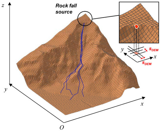
In order to cope with the limits characterising 2D modelling and associated “one-dimensional” hazard zoning, several 3D rock fall codes have been proposed lately [2,9,11,16,18,24], even though not many corresponding “two-dimensional” zoning procedures exist. Methodologies using 3D simulation results are meant to yield a more realistic description of rock fall propagation and hazard, thanks to the spatially distributed information they can provide. In these approaches, hazard is assessed over a plane (x, y) domain, starting from trajectory results obtained for a 3D topographic model. Some of the 3D codes proposed so far are even integrated into GIS tools, which can perform not only rock fall simulations but also the complete hazard assessment, up to the elaboration of a hazard map [2,9,11].
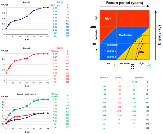
On the other hand, the above-mentioned procedures cannot take into account the effects of diffuse instabilities which generate multiple hazards occurring at the same site. When the instability is diffuse (e.g., linearly distributed or diffuse over a given area), the complexity of hazard assessment considerably increases. Each rock fall source may release a different number of blocks, which could also be characterised by different volumes and return periods. A methodology for hazard zoning should indeed be able to combine the effects associated to all the different sources threatening a given site. This problem is still currently unsolved, as 3D rock fall codes do allow for defining spatially distributed rock fall sources, but no procedure exists in 2D zoning methods for computing the corresponding effects on hazard assessment.
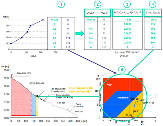
This paper aims at showing how the new hazard zoning methodology Cadanav [25,26], can be used for two-dimensional zoning. The methodology is based on a rigorous technique for combining rock fall energy and frequency, once information on failure frequency and trajectory simulations results are available. The procedure was introduced for one-dimensional zoning [25], with the goal of improving current hazard zoning techniques with respect to the points previously mentioned. Nevertheless, as limitations inherent to 2D rock-fall modelling/one-dimensional zoning remain, this paper illustrates how the applicability of Cadanav can be easily extended and based on 3D trajectory modelling. First, the basic principle and equations behind the 1D methodology are recalled, for introducing its extension to 2D. Then, applications are presented both for a simple topography underlying a linear cliff and for a complex topography, where three-dimensional effects on the motion of the blocks are very strong. For both topographies, several scenarios involving either localised or diffuse source areas are considered, in order to show the capabilities and flexibility of the methodology.
4. Applications to an Infinite Linear Cliff Model
Initially, the Cadanav methodology was applied to problems involving a simple topography underlying an “infinite” linear cliff. In this model, physical and mechanical characteristics (solid rock matrix and discontinuities) are assumed to be homogeneous all over the cliff length. First, a case study characterised by a single localised source area was analysed. Then, the applicability of the new procedure was extended to scenarios involving diffuse instabilities.
The topographic model used was created by building first a 2D slope profile on the (x, z) plane, and then by projecting this geometry into space, along the y-axis. Figure 4 shows the 2D profile adopted and the corresponding model built in 3D. The profile is 700 m long and starts at an altitude of 1006 m, ending at 677 m. It is characterised by 4 types of materials, defined based on the real slope characteristics this profile was inspired by: the first, up to x = 100 m and the second material, up to x = 110 m, represent two different types of rock, a limestone formation and a rock outcrop, respectively; the third (up to x = 400 m), a scree deposit coverage in a forested zone; the fourth, a grassy area (up to the end of the profile, at x = 700 m).
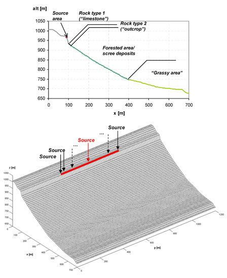
Figure 4.
Linear cliff model obtained from a 2D slope profile. The red line indicates the linear rock fall source area corresponding to the red point in the top figure.
The 3D model was then built based on a regular grid generated on the x-y plane, 700 m long in the x-direction and 1200 m in the y-direction. The grid is characterised by a cell size of 10 m × 10 m, which constitutes a good compromise between time for and amount of computations to be run for trajectory modelling and hazard zoning.
In all the analyses presented in this paper, the rock fall simulations were performed with the code EBOUL [24], assuming a cube-shaped block of 0.34 m3, with each side equal to 0.7 m. The hazard zoning was based on the Swiss intensity-frequency diagram.
4.1. Single Source Problem
In this application, a rock fall source located approximately at the centre of the model was considered, placed at (x, y, z) = (90 m, 610 m, 966.5 m). In terms of hazard scenario, a frequency of failure λf,2D equal to 0.02 (years−1·m−2) was assumed, that is, a failure frequency per source cell (10 m × 10 m) equal to λf,cell = 2 years−1. Regarding the rock fall simulations, 2500 trajectories were run from the source cell.
Figure 5 shows the results of the two-dimensional zoning. The hazard map obtained describes well the fact that, due to the simple structure of the topography, the hazard zones have a larger extent in the direction of the steepest path, in line with the propagation paths most likely to be followed by the blocks.
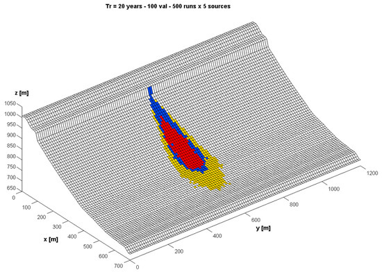
Figure 5.
Hazard zoning for a single source problem, performed according to the Swiss Guidelines, for a failure frequency of λf,2D = 0.02 (years−1·m−2), i.e., λf,cell = 2 years−1. Red: high hazard zone; blue: moderate hazard zone; yellow: low hazard zone.
4.2. Diffuse Source Problem
The first step towards the analysis of diffuse source problems was to test new Cadanav in a linearly distributed instability scenario. The topographic model considered in this application is the same infinite linear cliff introduced in the previous section. The source area was modelled by placing 52 source cells along the y-direction in the central part of the cliff, starting at x = 90 m (Figure 4). The total length of the unstable zone is then 520 m.
As the cliff can be considered homogeneous all over its length, it was assumed that (i) all the source cells have the same frequency of failure and (ii) each source releases blocks of the same shape and volume.
The hazard zoning was performed according to the principle of combination of the effects just illustrated in Section 3.3. A failure frequency λf,2D = 0.0025 (years−1·m−2) was assumed, i.e., λf,cell = 0.25 years−1 (which in other words means 13 blocks released per year from the whole cliff). From each of the 52 source cells, 500 trajectories were run.
Figure 6 shows the results of the hazard zoning. It can be noticed that in the central part of the map, i.e. sufficiently far from the borders of the source area, the hazard zones are defined by boundaries quite parallel to the cliff, as it should be expected in relation to the geometry of this problem.
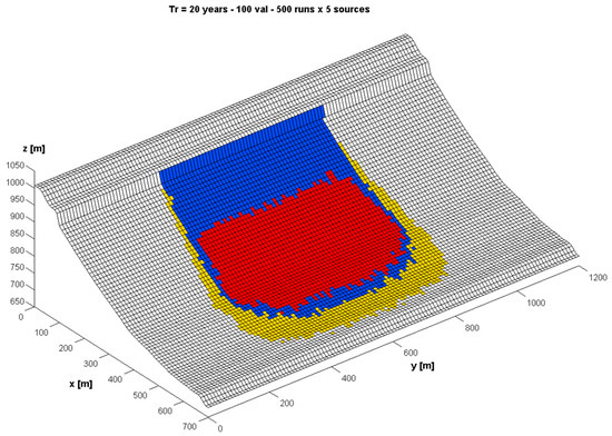
Figure 6.
Hazard zoning for a diffuse linear source problem, performed according to the Swiss Guidelines, assuming a failure frequency λf,2D = 0.0025 (years−1·m−2), i.e., λf,cell = 0.25 years−1.
4.3. 2D versus 1D Hazard Zoning
This case study was aimed at checking whether the new procedure (Section 3), once applied to a 3D infinite linear cliff topography, can actually yield, along any 2D profile of the slope, the same hazard zoning that the one-dimensional approach would provide (Section 2).
The x-z profile for the comparison was selected approximately at the centre of the unstable zone, at y = 610 m. This choice was done for ensuring that the two-dimensional hazard zoning obtained from 3D trajectories would be performed for a profile located sufficiently far from the starting and ending point of the source area, in order to avoid boundary effects.
For what concerns the rock fall propagation modelling, as the EBOUL code performs 3D simulations, a “pseudo-2D” trajectory study was carried out as follows. The computations were normally performed in 3D and afterwards, in order to virtually “restrain” the trajectories from going out of the vertical plane containing the profile selected, they were “projected” on the plane. In other words, the true y coordinate of each trajectory was set equal to the y coordinate of the profile, y = 610 m. Surely, such a way of proceeding carries with it a certain degree of approximation, but it seemed reasonable for comparison purposes.
Figure 7 shows the results for the 2D and 1D hazard zoning maps. Indeed, the two types of zoning provide results in quite good agreement. The position of the limits of each zone obtained according to the Cadanav methodology for one-dimensional zoning (Section 2) is located in the interval of variation provided by the methodology for two-dimensional zoning (Section 3). The slightly jagged contours of the 2D zoning map, which are related to a rather small number of trajectories computed per source cell (i.e., 500), show a maximum difference with the 1D hazard zoning of 20 m, i.e., 2 DEM cells. It is worth to keep in mind that some differences between the 1D and the 2D zoning results might be due to the approximation carried out when projecting the 3D trajectories on the y = 610 m profile.
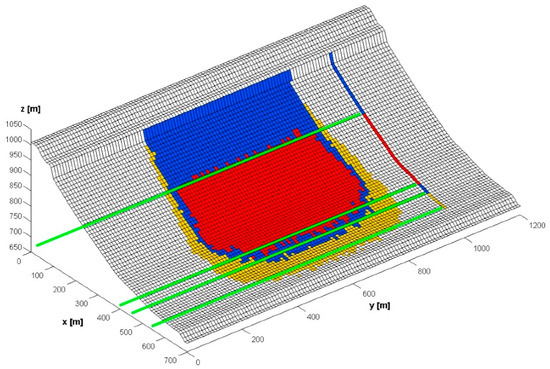
Figure 7.
2D and 1D hazard zoning for a failure frequency of λf,2D = 0.0025 (years−1·m−2), i.e., λf,cell = 0.25 years−1. The green lines help in comparing the position of the hazard zone boundaries obtained in each case.
4.4. Increasing Number of Rock Fall Sources
In the following application, Cadanav was applied by progressively increasing the number of source cells for the planar slope topography studied so far. The hazard analysis was performed for unstable areas constituted of 3, 6, 12, 26, 40, and 52 source cells, positioned symmetrically with respect to the central 2D profile of the cliff. A failure frequency per square metre of cliff of λf,2D = 0.0038 (years−1·m−2) was considered (i.e., λf,cell = 0.38 years-1 or Tf,cell ≃ 3 years) and, as done previously, 500 trajectories per source cell were run.
By looking at the results in Figure 8, a tendency to obtain linear boundaries parallel to the cliff in the “front” part of the hazard maps can be noticed (i.e., linear boundaries appear at those points of the map which are located the farthest from the source area, along the direction perpendicular to the cliff). When the size of the unstable areas is increased by adding more and more sources, the boundaries of the hazard zones move initially both down-slope and laterally (top and middle figures, representing the contribution of 3, 6, 12 and 26 source cells, respectively). Then, from a number of 26 sources on, the extent of the map increases only laterally (bottom figures, referred to 40 and 52 rock fall sources, respectively).
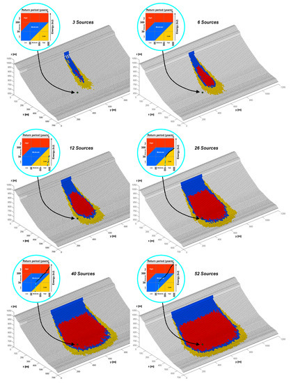
Figure 8.
Hazard zoning for increasing number of rock fall sources along a linear cliff, for a failure frequency of λf,2D = 0.0038 (years−1·m−2) (i.e., λf,cell = 0.38 years−1). The hazard curve superimposed to the intensity-frequency diagram helps in understanding how a point located relatively far from the source area can be affected by a hazard whose degree increases according to the combined effect of an increasing number of sources of instability.
Figure 9 illustrates schematically this feature, which is a consequence of the combination of the hazard zoning maps related to each single source element of the linear cliff. Normally, the boundaries of the hazard map expand both laterally and in the longitudinal direction, as much as the number of sources contributing to the hazard on the slope increases. However, at a certain distance from a given reference source, e.g., the central source in the figure, no contribution from other sources will occur in the area located below it, as none of the trajectories coming from far sources will reach this area. Accordingly, the hazard zone limits below the central source cannot move further down-slope. In contrast, (some of) these source cells which are “far” compared to the central can still contribute to the hazard generated by cells next to the central one. This makes the “front” of the hazard zone boundaries extend horizontally, as the map expands only towards its sides.
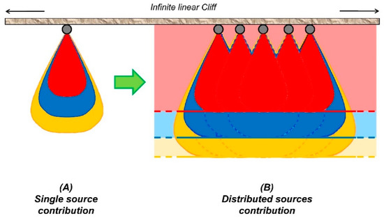
Figure 9.
(A) Schematic shape of the hazard zoning map due to each single source. (B) Hazard zoning map corresponding to the combination of the hazard related to all the sources of instability located along the linear cliff.
The Cadanav methodology proves therefore to be able to describe this aspect. In addition, by examining the hazard curves in Figure 8, obtained at a fixed cell located away from the axis of symmetry of the model, it can be observed how the hazard degree changes progressively from null to high as a consequence of the increasing number of sources considered (and the combination of their effects).
4.5. Combination of Rock Fall Hazards Characterised by Different Failure Frequencies
The objective of this analysis was to combine two different types of hazard characterised by different frequencies of failure, and to evaluate how the extent of the corresponding zoning map is influenced by the sum of their effects.
The two hazards taken into consideration are the linearly diffuse instability investigated previously (identified as Instability A), characterised by 52 source cells, and a localised instability, located at the centre of the topographic model (Instability B).
The failure frequency assumed for the linear instability is in this case of λf,2D = 0.002 (years−1·m−2) (i.e. λf,cell = 0.2 years−1 or Tf,cell ≃ 5 years), while the single instability is assumed to release blocks of the same volume as the other (0.34 m3), but characterised by a frequency of failure 10 times higher i.e., λf,2D = 0.02 (years−1·m−2) (i.e., λf,cell = 2 years−1 or Tf,cell ≃ 0.5 years).
Figure 10 shows the results for each of the two instabilities, separately, and then those referred to their combination.
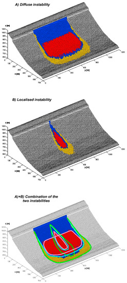
Figure 10.
Combination of a diffuse (λf,2D = 0.002 (years−1·m−2), i.e., λf,cell = 0.2 years−1) and a localised instability (λf,2D = 0.02 (years−1·m−2), i.e., λf,cell = 2 years−1) for a linear cliff slope geometry. The boundaries of each of the two separate hazard zoning maps (A) and (B) are superimposed to the map obtained from their combination, (A) + (B).
The hazard zone boundaries of the two separate instabilities are schematically traced (magenta, cyan and green lines for the red, blue and yellow zone boundaries, respectively) and overlaid to the map corresponding to their combination (bottom figure). It can be observed that the new Cadanav procedure quite well reproduces the fact that the hazard zoning map derived from the combination of two instabilities does correspond to more unfavourable conditions than those obtained by simply superimposing the hazard zones of each map, and tracing the envelope of the boundaries at equal level of hazard [8]. The limits of the hazard zones in the combined hazard map are in fact found farther down-slope if compared to this envelope. These results show reasonably well that the new Cadanav procedure is actually able to account for describing such a type of combination.
These results confirm the theoretical principle that, for an infinite linear cliff configuration, the boundaries of the hazard zones in the front part of a hazard zoning map are expected to be lines parallel to the linear source area [8].
5. Applications to a Complex Topography
This Section presents some examples of hazard zoning performed for a complex topography. At first, a single source problem was considered. Then, the effect of a channel-type topography on zoning was investigated, by defining a problem in which blocks were released from evenly distributed sources located along a semicircular-shaped unstable area.
5.1. Study Area: The Site of Les Crêtaux
The site selected for the following studies is the area of Les Crêtaux, in the Canton of Valais, Switzerland. The cliff is situated over the Rhone valley, near the village of Riddes (Figure 11). It is composed by carboniferous black schists and characterised by a mean dip of the general slope of about 40° [24].
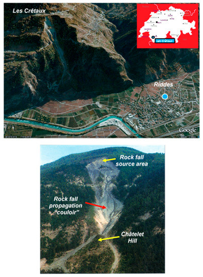
Figure 11.
Area of Les Crêtaux, Canton of Valais (Switzerland). Top: location and aerial view of the study site (sources: www.petiteviree.com, Google Earth). Bottom: front view of the rock fall source area and the corridor located just below (source: [17]).
The topography was modelled starting from a DEM with a cell size of 25 m × 25 m. Two different materials were defined along the slope for the rock fall simulations: one for modelling the corridor below the source area, where the blocks are driven after their detachment, and the other, for modelling the woods and the vineyards located just below the hill of Châtelet, which marks the bifurcation of the main corridor.
5.2. Single Localised Source Area
The new Cadanav procedure was first applied for assessing the hazard related to blocks falling from a single source cell, located at the top of the semicircular rock fall scar (Figure 12).
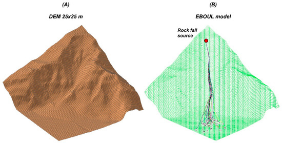
Figure 12.
(A) Topographic model obtained from a 25 m × 25 m digital elevation model (DEM). (B) Rock fall trajectory modelling performed with EBOUL, based on the DEM.
The hazard zoning was performed assuming a frequency of failure λf,2D = 0.04 (years−1·m−2) (i.e., λf,cell = 25 years−1 or Tf,cell = 0.04 years) and computing 17,000 trajectories for the same block volume and shape considered so far (cubic block of 0.34 m3).
Figure 13 shows the results obtained. It is easy to observe how the hazardous areas are concentrated along the corridor, which constitutes the preferential path followed by the blocks along their trajectories. Then, because of the presence of the Châtelet hill and the following flat zone, a greater dispersion of the trajectories occurs. Accordingly, the zoning map illustrates this trend, and the hazard levels decrease in the flat zone from the high value assessed in the corridor (red zone) down to null (white zone).
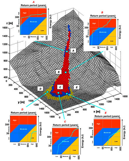
Figure 13.
Hazard zoning at Les Crêtaux, performed for a single source scenario characterised by a failure frequency λf,2D = 0.04 (years−1·m−2) (i.e., λf,cell = 25 years−1). The figure also shows the spatial evolution of hazard over the slope, at different points A, B, C, D and E, located at increasing distances from the source area.
In the same figure, hazard curves are also reported at different locations on the slope. Again, the curves effectively show how hazard evolves in space, at increasing distances from the source area. This superimposition shows that the limits of the zones in the combined map move downhill with respect to the single hazard maps.
5.3. Influence of a Change in the Failure Frequency Scenario on Hazard Zoning
The single source problem analysed in the previous section was considered also as a reference case study for testing how the Cadanav methodology describes changes in hazard zoning due to changes in the failure frequency of the events. Starting from the same failure frequency value (λf,2D = 0.04 (years−1·m−2)) and trajectory simulation results, the zoning was performed for three new values of failure frequency, which was decreased down λf,2D = 0.008 (years−1·m−2) (i.e., λf,cell = 5 years−1 or Tf,cell ≃ 0.2 years), 0.004 (years−1·m−2) (i.e., λf,cell = 2.5 years−1 or Tf,cell ≃ 0.4 years), and 0.0016 (years−1·m−2) (i.e., λf,cell = 1 years−1 or Tf,cell ≃ 1 year).
Figure 14 shows the hazard zoning maps obtained for the four scenarios. As expected, starting from the higher frequency value of the reference case, the extent of the endangered areas reduces for decreasing frequency values (i.e., increasing return period values), both in terms of length and width of the maps. With reference to the theoretical basis of Cadanav, illustrated in the first part of the article, the hazard curves consequently tend to move towards the right-hand side of the intensity-frequency diagram, i.e., towards low to null hazard degrees.
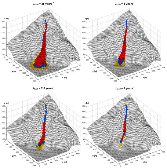
Figure 14.
Influence of a change in the failure frequency of failure on hazard zoning. The zoning was performed for failure frequencies of λf,2D = 0.04 (years−1·m−2) (i.e., λf,cell = 25 years−1), λf,2D = 0.008 (years−1·m−2) (i.e., λf,cell = 5 years−1), 0.004 (years−1·m−2) (i.e., λf,cell = 2.5 years−1), and 0.0016 (years−1·m−2) (i.e., λf,cell = 1 years−1).
5.4. Diffuse Source Area
The combined effect of several sources of instability was also investigated for a channel-type topography like the one found at Les Crêtaux. In this application, the hazard scenario modelled is a diffuse instability where the rock fall sources can be considered as evenly distributed along the (nearly) semicircular cliff located over the channel. In these conditions, all the trajectories released by the unstable zone are expected to be driven through the narrow area of the channel.
The distributed source area was modelled using nine source cells positioned rather evenly along the curvilinear rock fall scar and symmetrically with respect to the axis of the corridor (Figure 15, top).
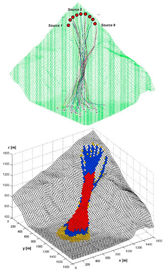
Figure 15.
Top: geometry used for the channel-type topography problem and overview on the rock fall paths predicted by EBOUL. Bottom: hazard zoning for the scenario assumed, performed by considering a frequency of failure of λf,2D = 0.0016 (years−1·m−2), i.e., λf,cell = 1 years−1.
The failure frequency was assumed as equal to λf,2D = 0.0016 (years−1·m−2) (i.e., λf,cell = 1 years−1), which means a total mean frequency of 9 events per year for the whole cliff (curvilinear source). For each source cell, 500 trajectories were computed, for a total of 4500 runs.
From the results illustrated in Figure 15, it can be observed that due to the “channel effect,” which brings blocks with high energy in the zone of convergence of (most of) the trajectories, the highest hazard values are found at the cells located in this area, as previously observed also in the single source problem.
It is also interesting to compare the hazard zoning maps obtained from a single source scenario (Figure 14, bottom right) and a diffuse scenario, for the same value of failure frequency per cell (λf,2D = 0.0016 (years−1·m−2) in these cases). As expected, the diffuse scenario is in these conditions much more unfavourable than the single source. Due to the combined effects of more rock fall sources, the map obtained covers a larger area (i.e., a larger area is potentially endangered) and the boundaries of each hazard zone are located farther down-slope.
6. Discussion
6.1. Further Assessment of the Results Obtained
The new Cadanav methodology proves to be quite a promising tool for tackling the problem of hazard zoning based on 3D rock fall modelling. If, on the one hand, it was tested only for two types of topographic configurations, the procedure performed well both in the validation tests run for the linear slope case and in the more realistic applications to a complex topography.
Regarding possible elements of validation, this is surely a complex issue for rock fall hazard zoning methodologies.
The best situations for possibly validating the results are constituted by any real site where a good amount of information is available, in terms of rock fall deposits/traces of impacts (for the calibration of rock fall trajectory codes) and historical records on past events (for estimating the failure frequency). In these conditions, the zoning maps obtained can be more soundly judged, based on what is observed on site. However, situations like these are not common, as most of the times data about trajectories and, mostly, failure frequency are lacking.
Nevertheless, solving simple theoretical benchmark problems can help also in a context like that of hazard assessment, for understanding whether a methodology responds correctly to well defined scenarios and topographic conditions specifically designed in input. If this is the case, the methodology can be expected to be relevant also for more complex and realistic scenarios, for which a sufficient amount of data for a thorough validation might be lacking. Under this point of view, the new Cadanav methodology performed the hazard zoning correctly in all the situations considered for validation purposes.
On the other hand, some of the benchmark problems analysed could be treated even more rigorously and provide a sounder check of the results obtained. In particular, regarding the comparison between one- and two-dimensional zoning, a more detailed approach could be used for improving the one-dimensional zoning from the results of the 3D trajectory calculation. For instance, a mathematical integration of the contribution of each source cell at each abscissa x of the profile selected could be performed (as theoretically formulated in Jaboyedoff et al. [8]), rather than simply “projecting” the trajectories on the vertical plane containing the profile and checking what zoning is obtained from this method (Section 4.3).
At the same time, more benchmark problems could also be studied, to strengthen the conclusions that the zoning provided by new Cadanav is theoretically sound. For example, the hazard zoning related to a block falling from the vertex of a conic topography could be considered [8], in order to check if the profiles of the hazard zone boundaries are well predicted in this condition too. In addition, the case of diffuse instabilities located along a semicircular source area over a channel-type topography (Figure 15) could be more thoroughly investigated as a benchmark problem. A perfect cone-shaped topography could be built and blocks be released from a perfectly curvilinear and continuous source area. This problem could further prove that the methodology accounts well for the contribution of several rock fall sources affecting the same cell.
Regarding the combination of more hazards occurring at the same site, illustrated in Figure 10, the results show reasonably well that the new Cadanav procedure allows for describing such a type of combination. Despite this, the effect is probably slightly less evident than it would be, were the length of the first instability larger. This would have meant having a greater extent of the part of the map characterised by boundaries parallel to the cliff for the diffuse instability. In these conditions, the “perturbation” of this scenario, due to the superimposition of the other, could have permitted to even more clearly see a localised area of overlaying.
Additionally, it must be remarked that multiple hazard scenarios were only tested assuming either the same block volume and failure frequency for all the sources of instability or by changing only the frequency of events from one instability type to another. The tests presented here did not account as well for the fact that changes in rock fall volume have to be in fact related to the changes in failure frequency, according to magnitude frequency relationships linking these two parameters [27]. In order to be complete in this sense, the methodology must also be able to deal with the more general case in which also the rock fall volume (influencing the total number of blocks released) and block volume change, which would possibly lead to define a more complex hazard combination procedure than the one used so far for the simpler problems treated.
Finally, in terms of practical application, the two-dimensional hazard analyses carried out in this work were run for cells of 10 m × 10 m (infinite linear cliff model) and 25 m × 25 m (Les Crêtaux). The latter especially is not really appropriate for local scale zoning and land use planning purposes, even though this cell size was sufficient to test the performing capabilities of the methodology. Analyses using smaller DEM cell sizes should be carried out in the future, in conditions closer to the needs of current hazard zoning practices.
6.2. Advantages of the Methodology
As shown in the first part of this article, the new Cadanav methodology proved to be easily applicable for two-dimensional hazard zoning, based on its original one-dimensional formulation. No significant modifications to the procedure were required, making the step from one-dimensional to two-dimensional zoning quite straightforward. The formulation of the whole procedure is therefore quite consistent—which was not fully the case, for instance, for the original version of the Cadanav methodology [8], not easily applicable starting from 3D trajectory modelling.
As a consequence, the same features and advantages of the one-dimensional approach [22,25] characterise as well its two-dimensional version.
First, the methodology is fully quantitative and takes into account all energy and related frequencies of occurrence values at each point of the slope. The hazard is therefore assessed based on a quite complete and objective procedure, which uses all the hazard descriptors required in hazard analyses [5,22,25,26]. The zoning provided is therefore sounder than in other methodologies as, actually, either existing procedures do not consider all the hazard descriptors in the assessment or many of them are semiquantitative/purely qualitative [25]—as mentioned in the introduction to this article.
Then, under the methodological point of view, the introduction of hazard curves has a twofold advantage. On the one hand, it yields a detailed method for assessing hazards, based on a rigorous coupling of energy and return period of the events. On the other hand, it provides a quick and effective representation of the evolution of hazard on the slope in space and time as well (i.e., changes in hazard at a given location of the slope according to changes in the failure frequency of the events).
Additionally, the two-dimensional formulation of new Cadanav keeps the strong points of the original methodology [20] already featured also in the new procedure when introduced for one-dimensional zoning [25]. In particular:
- the new procedure proved to take into account well the changes in hazard zoning due to changes in failure frequency (hazard zone boundaries moving up-slope towards the source area for increasing values of the return period of the events).
- the methodology seems to be not highly sensitive to the number of trajectories computed for hazard zoning and is not really influenced by the possible “extreme” propagation of a few blocks, obtained sometimes from the computations.
- the computational time required for hazard zoning, also for 3D topographies, depends only on the spatial discretisation of the problem and the number of rock fall trajectories processed. In particular:
- -
- for 1D zoning along 2D slope profiles, the time is proportional to the product of the number of control abscissas x2D along the slope profile, into which the profile itself is subdivided, and the number of 2D rock fall paths ntot,2D computed;
- -
- similarly, with regards to 2D zoning for 3D topographies, the computational time is a function of the number of elements constituting the mesh on the horizontal plane (x3D, y3D) and the number of 3D trajectory runs ntot,3D = nsource · ntraj,source performed.
According to the complexity of the problem in the sense specified above, therefore, the difference in the computational times between 1D zoning and 2D zoning, marked as t1D and t2D, respectively, can be expressed by the ratio:
In principle, applications to 3D topography involve more elements constituting the spatial domain and require more trajectories to be run (due to their higher variability). Despite this aspect, however, in all the cases tested, the times required for zoning computations remained extremely contained (i.e., a few minutes)—and way shorter, for instance, than those necessary for the performance of the 3D rock fall simulations.
Although applied according to the Swiss Guidelines all throughout this article, the new Cadanav procedure was not developed specifically for these recommendations. The construction of the hazard curves is independent of the intensity-frequency diagram used, so the new Cadanav is, in fact, applicable using any diagram. In this respect, it must be remarked that, currently, the Swiss Codes for hazard zoning have introduced a new hazard zone, classified as “residual hazard”, which is referred to events characterised by return periods higher than 300 years [28]. The Swiss intensity-frequency diagram is accordingly “extended” on the right-hand side by a hatched yellow-white area, which starts from T = 300 years and covers the whole spectrum of possible intensities (rock fall energy) along its y-axis (Figure 16). Adding this residual hazard level to the new Cadanav zoning methodology would be straightforward. However, this would first require the specification by the authorities of the maximum value of return period associated to this very low (i.e., residual) hazard.
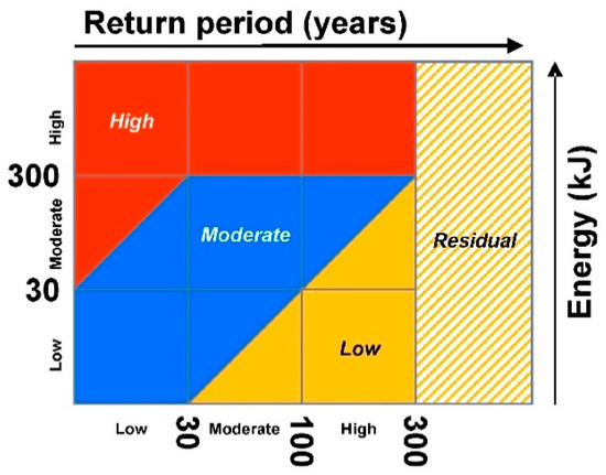
Figure 16.
Updated intensity-frequency diagram rock fall hazard zoning introduced by the Swiss Codes.
Finally, once the initial value of failure frequency has been defined and the raw rock fall simulation results are available, the new Cadanav methodology constitutes a procedure whose application is completely independent of the user, which makes it more transparent and systematically reproducible when compared to many other approaches.
7. Conclusions
The new Cadanav methodology was presented in this paper as a useful tool for rock fall hazard zoning based on 3D trajectory modelling. The procedure is fully quantitative and evaluates hazard consistently with the internationally accepted definition of landslide hazard. It constitutes a straightforward extension of the approach based on 2D simulations, rigorously combining available information on failure frequency and trajectory simulation results. The rock fall hazard zoning is obtained by energy-return period curves (hazard curves) built based on these data and used in combination with intensity-frequency diagrams.
The new methodology was applied to different types of hazard scenarios, involving simple and complex topographic models. Benchmark problems for validating the procedure were solved for simple “infinite linear cliff” configurations, characterised by a linearly distributed source area. More realistic scenarios were instead investigated for a channel-type topography, with remarkable topographic effects on the trajectory of the blocks. All the problems analysed included both single and diffuse source scenarios.
The methodology performed extremely well in all the conditions tested, providing sound results both for simple problems (single source) and for complex problems, in which combining the effect of multiple rock fall sources was required. Additionally, the new Cadanav proved to be able to take different hazards occurring at the same site into account in hazard zoning (at the current state of the research, when they are characterised by the same block size but different failure frequencies).
This new procedure constitutes a rigorous and robust hazard assessment tool and yields an objective zoning which is totally independent of the user and the intensity-frequency diagram considered.
Author Contributions
Conceptualization, J.M.A. and V.L.; methodology, J.M.A. and V.L.; software, J.M.A.; validation, V.L.; formal analysis, J.M.A. and V.L.; investigation, J.M.A. and V.L.; resources, J.M.A.; data curation, J.M.A. and V.L.; writing—original draft preparation, J.M.A.; writing—review and editing, J.M.A. and V.L.; visualization, J.M.A.; supervision, V.L.; project administration, V.L.; funding acquisition, V.L. All authors have read and agreed to the published version of the manuscript.
Funding
This work is based on a PhD thesis funded by the Marie Curie Research Training Network “Mountain Risks: from Prediction to Management and Governance” (6th Framework Program of the European Commission). The authors would like to thank the European Commission for the support to the research project.
Conflicts of Interest
The authors declare that they have no conflict of interest.
References
- Guzzetti, F. Landslide fatalities and the evaluation of landslide risk in Italy. Eng. Geol. 2000, 58, 89–107. [Google Scholar] [CrossRef]
- Crosta, G.B.; Agliardi, F. A methodology for physically based rockfall hazard assessment. Nat. Hazards Earth Syst. Sci. 2003, 3, 407–422. [Google Scholar] [CrossRef]
- Scavia, C.; Barbero, M.; Castelli, M.; Marchelli, M.; Peila, D.; Torsello, G.; Vallero, G. Evaluating Rockfall Risk: Some Critical Aspects. Geosciences 2020, 10, 98. [Google Scholar] [CrossRef]
- Fell, R.; Ho, K.K.S.; Lacasse, S.; Leroi, E. A framework for landslide risk assessment and management. In Landslide Risk Management; Taylor & Francis Group: London, UK, 2005; pp. 3–25. [Google Scholar]
- Fell, R.; Corominas, J.; Bonnard, C.; Cascini, L.; Leroi, E.; Savage, W.Z. on behalf of the JTC-1 Joint Technical Committee on Landslides and Engineered Slopes. Guidelines for landslide susceptibility, hazard and risk zoning for land use planning. Eng. Geol. 2008, 102, 85–98. [Google Scholar] [CrossRef]
- Rouiller, J.D.; Jaboyedoff, M.; Marro, C.; Phillippossian, F.; Mamin, M. Pentes Instables Dans le Pennique Valaisan. Rapport Final PNR 31; VDF: Zürich, Switzerland, 1998. [Google Scholar]
- Mazzoccola, D.; Sciesa, E. Implementation and comparison of different methods for rockfall hazard assessment in the Italian Alps. Landslides in Theory, Research and Practice. In Proceedings of the 8th International Symposium on Landslides, Cardiff, Wales, Balkema, Rotterdam, The Netherlands, 26–30 June 2000; pp. 1035–1040. [Google Scholar]
- Jaboyedoff, M.; Dudt, J.P.; Labiouse, V. An attempt to refine rockfall hazard zoning based on the kinetic energy, frequency and fragmentation degree. Nat. Hazards Earth Syst. Sci. 2005, 5, 621–632. [Google Scholar] [CrossRef]
- Lan, H.; Derek Martin, C.; Lim, H.C. RockFall Analyst: A GIS extension for three-dimensional and spatially distributed rockfall hazard modelling. Comput. Geosci. 2007, 33, 262–279. [Google Scholar] [CrossRef]
- Desvarreux, P. Problèmes posés par le zonage. In Lecture Notes from the Course Université Européenne d’été 2007: Éboulements, Chutes de Blocs—Rôle de la Forêt; Courmayeur, Italy, 2007. [Google Scholar]
- Guzzetti, F.; Crosta, G.; Detti, R.; Agliardi, F. STONE: A computer program for the three-dimensional simulation of rock-falls. Comput. Geosci. 2002, 28, 1079–1093. [Google Scholar] [CrossRef]
- Copons, R. Avaluaciò de la Perillositat de Caigudes de Blocs rocosos al Solà d’Andorra la Vella; Andorran Research Centre Press: St. Julià de Loria, Andorra, 2007. [Google Scholar]
- Choi, Y.; Lee, J.; Lee, J.; Park, H.D. Engineering geological investigation into rockfall problem: A case study of the Seated Seokgayeorae Image carved on a rock face at the UNESCO World Heritage site in Korea. Geosci. J. 2009, 13, 69–78. [Google Scholar] [CrossRef]
- Pfeiffer, T.J.; Higgins, J.D.; Andrew, R.D.; Schultz, R.J.; Beck, R.B. Colorado Rockfall Simulation Program Version 3.0a User’s Manual; Colorado Department of Transportation: Denver, CO, USA, 1995.
- Stevens, W.D. RocFall: A Tool for probabilistic analysis, design of remedial measures and prediction of rockfalls. Master’s Thesis, University of Toronto, Toronto, ON, Canada, 1998. [Google Scholar]
- Scioldo, G. Rotomap: Analisi statistica del rotolamento dei massi. In Guida Informatica Ambientale; Patron: Milano, Italy, 1991. [Google Scholar]
- Interreg IIc. Prévention des Mouvements de Versants et des Instabilités de Falaises: Confrontation des Méthodes d’étude d’éboulements Rocheux dans l’arc Alpin; Interreg Communauté Européenne: Aosta, Italy, 2001. [Google Scholar]
- Dorren, L.K.A. Rockyfor3D Revealed—Description of the Complete 3D Rockfall Model, ecorisq Paper. Available online: https://www.ecorisq.org/publications/tools-manuals/rockyfor3d-user-manual (accessed on 26 June 2020).
- Hantz, D. Quantitative assessment of diffuse rock fall hazard along a cliff foot. Nat. Hazards Earth Syst. Sci. 2011, 11, 1303–1309. [Google Scholar] [CrossRef]
- Abbruzzese, J.M.; Sauthier, C.; Labiouse, V. Considerations on Swiss methodologies for rock fall hazard mapping based on trajectory modelling. Nat. Hazards Earth Syst. Sci. 2009, 9, 1095–1109. [Google Scholar] [CrossRef]
- Raetzo, H.; Lateltin, O.; Bollinger, D.; Tripet, J.P. Hazard assessment in Switzerland—Codes of Practice for mass movements. Bull. Eng. Geol. Environ. 2002, 61, 263–268. [Google Scholar]
- Labiouse, V.; Abbruzzese, J.M. Rockfall hazard zoning for land use planning. In Rockfall Engineering; Lambert, S., Nicot, F., Eds.; John Wiley & Sons: New York, NY, USA; London, UK, 2011; pp. 211–253. [Google Scholar]
- Spang, R.M.; Krauter, E. Rockfall simulation—A state of the art tool for risk assessment and dimensioning of rockfall barriers. In Proceedings of the International Conference on Landslides—Causes, Impacts and Countermeasures, Davos, Switzerland, 17–21 June 2001; pp. 607–613. [Google Scholar]
- Descoeudres, F.; Zimmermann, T. Three-dimensional dynamic calculation of rockfalls. In Proceedings of the 6th International Congress of Rock Mechanics, Montreal, QC, Canada, 30 August–3 September 1987; pp. 337–342. [Google Scholar]
- Abbruzzese, J.M.; Labiouse, V. New Cadanav methodology for quantitative rock fall hazard assessment and zoning at the local scale. Landslides 2013, 11, 551–564. [Google Scholar] [CrossRef]
- Abbruzzese, J.M. Improved Methodology for Rock Fall Hazard Zoning at the Local Scale. Ph.D. Thesis, École Polytechnique Fédérale de Lausanne (EPFL), Lausanne, Switzerland, 2011. [Google Scholar]
- Hungr, O.; Evans, S.G.; Hazzard, J. Magnitude and frequency of rock falls along the main transportation corridors of southwestern British Columbia. Can. Geotech. J. 1999, 36, 224–238. [Google Scholar] [CrossRef]
- OFEV (Office Fédéral de L’Environnement). Protection Contre Les Dangers Dus Aux Mouvements de Terrain. Aide à l’exécution Concernant la Gestion des Dangers dus Aux Glissements de Terrain, Aux Chutes de Pierres et aux Coulées de Boue; Office Fédéral de L’environnement: Berne, IN, USA, 2016.
Publisher’s Note: MDPI stays neutral with regard to jurisdictional claims in published maps and institutional affiliations. |
© 2020 by the authors. Licensee MDPI, Basel, Switzerland. This article is an open access article distributed under the terms and conditions of the Creative Commons Attribution (CC BY) license (http://creativecommons.org/licenses/by/4.0/).
