Investigating the Behavior of an Onshore Wall and Trench Combination Ahead of a Tsunami-Like Wave

Abstract

This study investigates a wall and trench combination to identify its benefits as a defense measure against an overtopping tsunami-like wave. The study focuses on several arrangements and geometries of a wall and trench combined structural system, located on the shoreline. The structural system is assessed via a numerical model, which is initially calibrated by physical experiments of tsunami-like wave transformations. A dam break event is used to model a tsunami-like wave interaction with the structures. Resulted wave properties are investigated to identify the behavior of the structural system from the viewpoint of structure geometry and configuration. The results of the study clearly show that the proposed structure combination can effectively reduce the impact of tsunami-like waves, better than a single sea wall defense system. This is achieved by reducing both wave run-up and wave induced current velocities at the lee side of the structure.

1. Introduction

Oceanic tsunami-wave trains are generally triggered by underwater earthquakes, which travel from deep waters and eventually break near the shoreline. These wave -trains may form a sequence of turbulent bores that propagate toward shallow water or alternatively collapse upon near shore structures. The wave train sends a surge of water, sometimes reaching run-up heights of over 30 m in to land. The massive energy of the wave front can cause widespread destruction when they land onshore with in a very short period of time.

The amplitude of a typical tsunami wave in the open ocean is rather small (normally from 1 to 30 cm) [1]. Its length can reach hundreds of kilometers, which is much greater than the depth of the ocean. As this wave approaches the shore with a decreasing speed, its amplitude increases dramatically, which can lead to the destruction of various facilities in the coastal zone due to flooding.

Coastal dikes and seawalls are the most popular defense structures against tsunamis, which are commonly used across the world. Countries like Japan have strongly invested in building such structures along its tsunami vulnerable areas, especially since 2011 Great East Japan Tsunami, which has been identified as one of the largest natural disasters in recent history. Some of these structures can reach a height of 17 m with a length of several kilometers along the East coast of Japan [2]. There are however increasing concerns on the disadvantages that these structures have towards socially and environmentally sensitive areas due to the defensive position of these massive walls.

Tsunami interaction with defense structures like seawalls was observed in largely during recent disaster events like the 2011 Great East Japan Tsunami. During these events, the failure of strong hard measures gave another perspective to the field of tsunami defense. Even with a world-class disaster warning system, the massive destruction of 2011 Great East Japan Tsunami, could not be mitigated successfully [3]. It demonstrated that current popular protective structures, such as seawalls, dikes and breakwaters, cannot be the only countermeasures to protect coastal communities from serious natural disasters [4].

With these experiences, building giant defense structures against tsunami is somewhat questionable. Although the structure can provide protection for some extent during a disastrous events, it generates numerous impacts on social and environmental likelihood. Keeping a giant wall along the shoreline that would be necessary only for a rare event is also questionable, as it would cut-off the social and economic activities of locals that are directly bonded with the ocean. However, opposition between these differing forms of infrastructure was eventually resolved through gradually negotiation in which the sea wall and the boundary markers could complement one another. This situation highlights the intricate, transformable relation between visible and invisible forms of infrastructure [5].

From this, a need has been raised to enhance the effectiveness of conventional seawalls with a number of researchers having focused on improving coastal defense against tsunami, by applying different type of structures and solutions in addition to sea walls and sea dikes.

The study of Hsiao and Lin [6] on tsunami-like solitary waves impinging and overtopping an impermeable seawall is one example that can be given as a pre-2011 tsunami disaster study. Where he focused on describing three typical cases of a tsunami wave interacting with a seawall—a turbulent bore rushes inland and subsequently impacts and overtops the seawall (Type 1); a wave directly collapses on the seawall and then generates overtopping flow (Type 2); and a wave straightforwardly overtops the seawall crown and collapses behind the seawall (Type 3). Hsiao and Lin [6] provide an insight in to tsunami wave overtopping a seawall descriptively. In addition to Hsiao and Lin’s [6] work, a study was carried out by Esteban et al. [7] on overtopping of coastal structures by tsunami waves, which discusses tsunami overtopping on different types of seawalls.

Tsunami reduction by hybrid structures have also been focused by various researchers. For example, the experimental study by Zaha, Tanaka and Kimiwada [8] investigated various combinations of embankment, moat (trench) and emergent vegetation to evaluate their effectivity as a tsunami defense system. When the trench is located at the lee side of the wall, it resulted in significant reduction effect of the fluid force index by decreasing the overtopping flow velocity from the embankment.

Energy reduction of a tsunami current through another hybrid defense system was experimentally evaluated by Muhammad and Tanaka [9]. The study focused on a combination of embankment wall and a coastal forest which is located at the lee side of the wall.

The Buckingham Canal in Andhra Pradesh in India was a significant mitigating factor, saving the lives of numerous fishermen, particularly in coastal areas around Chennai [10], during the 2004 Indian Ocean tsunami. This information led to the discussion that canals can be an effective countermeasure to protect coastal areas from tsunami strike.

Further, during the 2011 Great East Japan Tsunami, Tokida and Tanimito [11] showed that the water pool made by the flood stream of a tsunami, called a dug pool, can be effective in reducing the tsunami flow velocity. In spite of that, Dao et al. [12] carried out a series of numerical experiments to investigate the sensitivity and effects of ashore-parallel canal to reduce a tsunami energy. Dao’s [12] results showed that a canal parallel to the shoreline has significant effect in reducing tsunami energy and plays an important role in the mitigation of tsunami impacts. Although the study of Dao et al. [12] focused on a cannel on land, it showed some promising outcomes of a wall trench system that would significantly be effective in reducing current speeds of a tsunami-like wave.

Rahman et al. [4] carried out an experimental and numerical study to investigate canals as a mitigation of a tsunami and concluded a positive reduction of tsunami waves by incorporating a narrow canal, orientated perpendicular to the wave direction.

2. Focus and Objectives

By looking at the previous studies, it can be noticed that the researchers have mostly considered either vertical or embankment type seawalls, vegetation and trenches/canals or different combinations of those against tsunami-like waves. However, the geometrical optimizations of these structures were not evaluated much in most of the cases. Silva and Araki [13] conducted a study to investigate the behavior of a submerged wall and trench system near the shore, which discussed how the structure configuration and geometry affects an approaching tsunami wave. Nevertheless, the geometrical optimization of a combined wall and trench system that would significantly influence the run-up and inundation of a tsunami-like wave as it approaches onshore has rarely been studied.

For this study, focus is placed more on a combined wall and trench system on the shoreline, which would act as a tsunami defense structure. A set of numerical simulations following physical experiments were performed through a computational fluid dynamics (CFD) model that predicts the run-up heights of a tsunami-like wave on a sloping beach in accordance to the dimensions of a submerged wall and trench systems. This was followed by performing different variations to the run-up processes considering different geometries to the structural system being investigated.

3. Materials and Methods

3.1. Experimental Setup

Firstly, an experiment was setup in a 2D flume (wave tank) to physically simulate a dam break event. The purpose of this experiment was to fine-tune the numerical setup, which is explained in the next stage. The schematic diagram of the experiment is shown in Figure 1. The dimensions of the flume are 44 m, 0.7 m, 0.9 m (length, width, depth). The difference of water level between reservoir and the experimental tank is initially maintained to be 0.13 m. The flume length of 44 m is comprised of two slopes—1/40 slope and 1/100 slope.

By considering, geometric, kinematic and dynamic similarities, a scale ratio of 0.0125 (1:80) is assumed to represent reality. The initial conditions were decided from a series of trial and error experiment cases to generate a tsunami-like wave having a wave height of about 7 m (~8.75 cm in model scale) at the shoreline.

Current speeds were also measured and considered when deciding the initial conditions. The selected initial conditions or the water column of 0.13 m at the reservoir end, generated a maximum current speed on the shore of about 6.25 m/s (~0.7 m/s in model scale) when reaching the shore. Historical records of the 2004 Indian Ocean tsunami and the 2011 Great East Japan Tsunami were taken into consideration when deciding the initial conditions for the experimental setup. The observed water level data during the 2011 Great East Japan Tsunami can be downloaded from the official website of Nationwide Ocean Wave Information Network for Ports and Harbors (NOWPHAS) [14]. In the case of the 2004 Indian Ocean tsunami, the observed tide gauge data can be found in the publication of Grilli et al. [15]. These were both considered for this study, however, these data recordings have significant deviation due to dependences on the location, measuring depth and the event itself, it was decided to follow a 7 m (~8.75 cm in model scale) tsunami wave height near the shoreline. This provided a realistic representation of an average tsunami wave height in the modelling environment.

Once the initial water condition was steady at the reservoir end, the gate was raised manually to generate a dam break waveform. The transforming waveform was measured by several water level gauges at different locations (A, B, C, D and E) along the wave tank. In addition, the current speeds of the upcoming wave were measured at two locations (B and C) near the shoreline. An electromagnetic current meter was used to measure current speeds. The location of each gauge is also given in Figure 1. Readings of the water level gauges and current meters were used to calibrate the numerical model in the next stage.

3.2. Numerical Setup

The open source CFD code pack, OpenFOAM^®, was used to set up the experiments numerically. OpenFOAM^® features a three-dimensional, two-phase (Reynolds Averaged Navier Stokes) RANS solver called “interFoam,” which was presented in detail in Santiago’s doctoral dissertation [16]. The dynamics is solved for both water and air in all the cases presented in this paper, which is an advantage, as it is a more complete approach. Water is simulated with density ${\rho }_{water}$ = 1000 kg/m³ and kinematic viscosity ${\upsilon }_{water}$ = 10⁻⁶ Pa/s, while air has density ${\rho }_{air }$ = 1 kg/m³ and kinematic viscosity ${\upsilon }_{air}$ = 1.48 × 10⁻⁶ Pa/s.

A descriptive explanation of the background of the OpenFOAM^® interFoam solver can be found on Lopes’s doctoral dissertation [17]. The mathematical and numerical background of the solver can be found in detail from the works of Jasak [18], Ubbink and Issa [19] and Rusche [20]. The governing equations include continuity and momentum equations, respectively given in Equations (1) and (2):

$$\frac{\partial u_i}{\partial x_i}=0$$

(1)

$$\frac{\partial \rho u_i}{\rho t}+u_j\frac{\partial \rho u_i}{\partial x_j}=-\frac{\partial p^{*}}{\rho x_i}-g_j{x}_i\frac{\partial \rho }{\rho x_i}+\frac{\partial }{\rho x_j}\left(2\mu S_{ij}\right)+{\sigma }_{T}K\frac{\partial \alpha }{\rho x_i},$$

(2)

where $x_i$ are the Cartesian coordinates, $u_i$ are the mean components of the velocities, $p^{*}$ is the pressure minus the hydrostatic potential $\rho g_j{x}_i$, $\rho$ is the fluid density (which takes the constant value ${\alpha }_{water}$ in the water and jumps at the interface to the constant value ${\alpha }_{air}$ in the air phase), $g_j$ is the gravitational acceleration, $\mu =\rho \upsilon$ is the dynamic molecular viscosity ($\upsilon$ being the kinematic viscosity) and $S_{ij}$ is the mean strain rate tensor given by

$$S_{ij}=\frac{1}{2}\left(\frac{\partial u_i}{\partial x_j}+\frac{\partial u_j}{\partial x_i}\right).$$

(3)

The effect of surface tension ${\sigma }_T$ is accounted in the last term in Equation (2). where $\alpha$ is the indicator field introduced in volume of fluid method, which takes value 0 in air and 1 in water and $K$ is the local surface curvature. $\alpha$ can be defined in terms of the density as

$$\alpha =\frac{\rho -{\rho }_{air}}{{\rho }_{water}-{\rho }_{air}}.$$

(4)

Similar to density, any fluid property, $\mathsf{\Phi }$, can be expressed in terms of $\alpha$

$$\mathsf{\Phi }=\alpha {\mathsf{\Phi }}_{water}+\left(1-\alpha \right){\mathsf{\Phi }}_{air}.$$

(5)

To calculate the evolution of $\alpha$ the continuity equation can be applied as follows.

$$\frac{\partial \alpha }{\partial t}+\frac{\partial \alpha u_i}{\partial x_j}=0.$$

(6)

“Multidimensional Universal Limiter with Explicit Solution” (MULES) limiter, which is a numerical interface compression method with limited phase fluxes is applied to keep the sharp interface between two fluids (air and water). The compression is calculated by adding another term (7) to Equation (6).

$$\frac{\partial \alpha }{\partial t}+\frac{\partial \alpha u_i}{\partial x_j}+\frac{\partial }{\partial x_j}\left(\alpha \left(1-\alpha \right)u_j^r\right)=0,$$

(7)

where $u_j^r$ is modelled as a relative velocity used to compress the interface. More information on the numerical implementation, can be found in Deshpande’s [21] performance evaluation of interFoam solver.

The numerical model was set up to simulate the experimental dam break event. The domain is constructed in a 3D environment. Depth contours were introduced into the grid by defining the same depth levels from the experiment. The domain is then introduced into interFoam module by applying a set of initial conditions (13 cm water column at the reservoir end) to calculate the evolution of the wave generated by the dam break event. The complete flume is replicated in 3D at the initial stage and then performed 3D to 2D conversion by extruding cells of the Y direction. The longest length of the flume corresponds to the X axis and it is meshed varying the cell discretization, which allows for better resolution in critical zones as near the structures, while providing adequate resolution for other zones where dynamics are less restrictive. Maximum resolution in X and Y directions were maintained to 10 cm. Higher resolution is applied at the shoreline area by decomposing the domain. This disposition totals ~0.4 million cells. The inbuilt meshing tool, “snappyHexMesh” was used for further smoothing and rearranging of cells.

Turbulence is modelled using $k-\epsilon$ turbulence model. $k$ and $\epsilon$ represents the turbulent kinetic energy and turbulent dissipation rate respectively. To calculate $k$ and $\epsilon$ for the initial conditions, the expressions given by Cox. D. et al. [22] were used and are listed in Equations (8) and (9).

$$k=\frac{3}{2}{\left(I\left|U_{ref}\right|\right)}^2$$

(8)

$$\epsilon =\frac{C_{\mu }^{0.75}{k}^{1.5}}{L} ,$$

(9)

where, $I$ is the turbulence intensity, $U_{ref}$ is the reference flow speed, $C_{\mu }$ is a model constant equal to 0.09 [22] $L$ is the reference length scale. An average reference velocity is considered (0.4 m/s), at the initial stage of dam break event for $U_{ref}$. A turbulent intensity $\left(I\right)$ of 0.1 (10%) was applied by considering the suggestions of Park. et al. [23]. $L$ was calculated by $L=0.04d$ [22], where $d$ is the reference depth given as 0.25 m was assumed at the initial stage considering varying depth of the flume (from ~0.5 m to 0). The calculated Initial values for $k$ and $\epsilon$ were 0.0023 m²/s² and 0.0548 m²/s³ respectively. Other important interFoam parameters that were applied in the simulations are given in

Table 1. interFoam parameters.

ControlDict	Scheme/Value
adjustTimeStep	true
maxCo	0.5
maxAlphaCo	0.5
fvSchemes	Scheme/Value
ddt	Euler
grad	Gauss linear
div(rhoPhi,U)	Gauss linearUpwind grad(U)
div(phirb, alpha)	Gauss linear
div(phirb, alpha)	Gauss linear
div(phi,k)	Gauss upwind
div(phi,epsilon)	Gauss upwind
laplacian	Gauss linear corrected
interplolation	linear
snGrad	corrected
fvSolution	Scheme/Value
alpha.water. (solver, tol, relTol)	smoothSolver, 1 × 10−8, 0
pcorr(solver, prec, tol, relTol)	PCG, DIC, 1 × 10−8, 0
p_rgh(solver, prec, tol, relTol)	PCG, DIC, 1 × 10−8, 0
U|K|epsilon	smoothSolver, 1 × 10−8, 0

.

Water level variations and current velocities were extracted from simulation results at the same gauge locations as the experiment and were compared with recordings from the experiment. Plots of comparison are given under results and discussion.

3.3. Simulations with Onshore Structures

The onshore structures were then introduced to the numerical domain by altering the bottom profile. Several types of structures were assessed including a single vertical seawall and wall and trench systems with different geometries. The orientations and real scale dimensions of each structural system are listed in

Table 2. Description of simulation cases with details of onshore structures (in real scale).

Case No.	Description	Wall Height (cm)	Wall Width (cm)	Trench Depth (cm)	Trench Width (cm)	Spacing (cm)
1	Without Structures	-	-	-	-	-
2	Single wall	6.25	12.5	-	-	-
3	Wall-trench	6.25	12.5	6.25	12.5	6.25
4	Wall-trench	6.25	12.5	6.25	12.5	12.5
5	Wall-trench	6.25	12.5	6.25	12.5	18.75
6	Wall-trench	6.25	12.5	6.25	6.25	12.5
7	Wall-trench	6.25	12.5	6.25	12.5	12.5
8	Wall-trench	6.25	12.5	6.25	18.75	12.5
9	Wall-trench	6.25	6.25	6.25	12.5	12.5
10	Wall-trench	6.25	12.5	6.25	12.5	12.5
11	Wall-trench	6.25	18.75	6.25	12.5	12.5
12	Wall-trench	6.25	12.5	3.125	12.5	12.5
13	Wall-trench	6.25	12.5	6.25	12.5	12.5
14	Wall-trench	6.25	12.5	9.375	12.5	12.5

. The schematic diagram of the wall and trench system is given in Figure 2.

3.4. Comparing the Combined Wall and Trench System with Single Seawall System

The results of the tsunami interaction with combined wall and trench systems were compared against the tsunami interaction ahead of a single sea wall system. A typical embankment type sea wall was considered when comparing with the wall and trench systems. Figure 3 show the layout of the single wall and the wall and trench system that were compared with each other. The height of the wall was the only variable parameter in the comparison.

Table 3. Description of simulation cases with the details of onshore structures (in model scale).

Case No.	Description	Wall Height (cm)	Wall Width (cm)	Trench Depth (cm)	Trench Width (cm)	Spacing (cm)
15	Single wall	5	12.5	-	-	-
16	Single wall	6.25	12.5	-	-	-
17	Single wall	7.5	12.5	-	-	-
18	Single wall	3.75	12.5	6.25	12.5	6.25
19	Wall-trench	5	12.5	6.25	12.5	6.25
20	Wall-trench	6.25	12.5	6.25	12.5	6.25
21	Wall-trench	7.5	12.5	6.25	12.5	6.25
22	Wall-trench	5	12.5	-	-	-

gives the simulation cases and the geometries of each structure combination.

3.5. Evaluating the Behavior of the Structure Ahead of Different Tsunami Conditions

Thus far, the same tsunami condition (water level difference at the reservoir and the wave tank —13 cm) has been used for all of the simulation cases. However, when looking at the results of simulation cases with variable spacing between the wall and the trench, it was found that the combined wall and trench structure combination behaved quite differently ahead of different tsunami levels when the spacing between the wall and the trench changed. Therefore, it was decided to investigate those observations by applying the structure systems with variable spacings in to different tsunami conditions.

Table 4. Description of simulation cases with the details of onshore structures (in model scale).

Tsunami Condition (cm)				Description	Wall Height (cm)	Wall Width (cm)	Trench Depth (cm)	Trench Width (cm)	Spacing (cm)
11	13	15	17
Case no.
23	24	25	26	Wall-trench	6.25	12.5	6.25	12.5	0
27	28	29	30	Wall-trench	6.25	12.5	6.25	12.5	2.5
31	32	33	34	Wall-trench	6.25	12.5	6.25	12.5	5
35	36	37	38	Wall-trench	6.25	12.5	6.25	12.5	6.25
39	40	41	42	Wall-trench	6.25	12.5	6.25	12.5	7.5
43	44	45	46	Wall-trench	6.25	12.5	6.25	12.5	10
47	48	49	50	Wall-trench	6.25	12.5	6.25	12.5	12.5
51	52	53	54	Wall-trench	6.25	12.5	6.25	12.5	18.75

gives the details of the simulation cases of this section. Each simulation case was subjected to four different tsunami conditions (11 cm, 13 cm, 15 cm and 17 cm) respectively.

4. Results and Discussion

This section is divided by subheadings to provide a concise and precise description of the results of physical experiments and simulations, their interpretation and conclusions against certain aspects.

4.1. Comparison of Wave Transformation

Figure 4, Figure 5 and Figure 6 show the comparison between measured and simulated water level variations at each gauge location with elevation measured from the most bottom of the flume (Bottom left in Figure 1). From the figures below, it can be proposed that the numerical model is capable of reproducing the water level variations, which are generated by the striking wave. High frequency oscillations of the free surface were also reproduced well before wave breaking. However, higher deviation is observed once the wave reached onshore.

Figure 7 and Figure 8 show the comparison of measured and simulated current velocity variations at gauge locations B and C. As a result of limited resources and some practical difficulties, the authors measured current velocity variations only at gauge locations B and C. By examining both figures, it is clear that the shape of the current velocity variations were also reproduced comparatively well by the numerical model. Even though there is a deviation at the end of the wave bore, the maximum current velocities were accurately predicted by numerical simulations.

4.2. Assessment of Onshore Structures

This section discusses the results of simulation cases of differing structures. The water level variations and current velocity variations at each gauge location are given in the following figures. Figure 9 and Figure 10 represents the variations of parameters at location D (lee side of the structure) for Cases 1 to 5; previously described in detail in Section 3.2.

Case 1 simulation is without onshore structures. Case 2 simulation is with a single vertical seawall. Case 3 simulation is with a combined wall and trench system with a spacing of 6.25 cm. For Cases 4 and 5, the spacing between the wall and the trench was increased to 12.5 cm and 18.75 cm respectively (refer to Table 2 for details) while maintain consistence of all other geometrical parameters.

Figure 9 clearly shows a reduction of maximum water level variation after applying onshore structures. The wall and trench system with 6.25 cm spacing suppressed the upcoming wave better than other structural system combinations. This is because overtopping waves directly collapse in to a lee side trench (discussed in detail under Section 4.4). Figure 9 also shows that both of the other wall and trench systems reduced the free surface variation better than the single seawall system.

Current velocity variations (shown in Figure 10) of the wall and trench cases do not show a significant reduction when compared to the single wall system. However, arrival time of the wave had increased in all other wall and trench cases.

Figure 11 and Figure 12 give a comparison of water level variations and current velocity variations respectively at location D for Cases 1, 2, 6, 7 and 8. The width of the trench was increased gradually in Cases 6, 7 and 8 to assess the impact while maintaining the same geometric parameters of the structural system.

Similar to Figure 9, Figure 11 indicates a reduction of maximum water level variation after applying onshore structural systems. The wall and trench system with the widest trench suppressed the upcoming wave better than any other structural system combinations. Figure 11 also showed that both of the other wall and trench systems reduced the free surface variation better than the single seawall system.

Current velocity variations (shown in Figure 12) of wall and trench cases also reflect suppressed values. This is also the case for the arrival time of the wave, which increased in all wall and trench cases when compared to the simulation for a single seawall. The simulation showed that the case with the widest trench provided the most effective suppression.

Figure 13 and Figure 14 both give a comparison of the water level variations and the current velocity variations respectively at location D for Cases 1, 2, 9, 10 and 11 respectively. The width of the wall was increased gradually in Cases 9, 10 and 11 to assess the impact while maintaining the same geometric parameters of the structural system.

Similar to Figure 11, Figure 13 shows a reduction of the maximum water level variation after applying structures onshore. The wall and trench system with the widest wall suppressed the upcoming wave better than other structure combinations. All the other wall and trench systems also reduced the free surface variation better than that of a single seawall system.

Though current velocity variations (shown in Figure 14) of all the simulation cases with a wall and trench system do not show a significant reduction when compared to the simulation case with a single wall; the times of tsunami arrival had increased for all cases. The case with the widest wall appears to be the most effective structure from the viewpoint of water level reduction and wave arrival time.

Figure 15 and Figure 16 both give a comparison of water level variations and current velocity variations respectively at location D for Cases 1, 2, 12, 13 and 14 respectively. The depths of the trench were increased gradually in Cases 12, 13 and 14 to assess the impact while maintaining the same geometric parameters of the structural system.

Similar to other comparisons previously presented, Figure 15 shows a reduction of the maximum water level variation after applying structures onshore. The wall and trench system with the deepest trench had suppressed the upcoming wave better than any other structure combinations. All the other wall and trench systems had also damped the free surface variation better than a single seawall system. The current velocity variations (shown in Figure 16) of the simulation cases with wall and trench systems also had damped values compared to that of the simulation case with a single seawall. Additionally, the arrival times of the wave had increased for all the simulation cases with a wall and trench system compared to that of the simulation with a single seawall. The simulation case with the deepest trench presented the most effective wave damping.

Next stage of the investigation was to assess the inundation that had occurred by the striking wave at the 1:100 beach slope for each simulation case. Wave induced inundations for a given time (240 s of simulation time) were plotted and presented in Figure 17, Figure 18, Figure 19, Figure 20 and Figure 21. The y-axis of these figures is scaled to$\alpha$, which is a dimensionless fraction delaminating air and water used in the simulations. Water is represented when $\alpha =1$ and air is represented when $\alpha =0$. Therefore, the interface between 1 and 0 at the beach slope can be identified as the point at where the water wave is reached on the 1/100 beach slope at a given time. $\alpha$ values between 0 and 1 indicates the air-water mixture at the fluid transition interface.

Figure 17 was plotted to compare simulations with wall and trench systems of different spacings between the wall and the trench (Cases 1 to 5), which showed the maximum wave inundation along the x-axis for a given time.

By looking at the run-up reduction, it is clear that the wall and trench system with a 6.25 cm spacing produced the most effective suppression of an upcoming wave. Clearly, all cases with wall and trench systems resulted in better inundation reduction compared to that of the case for a single seawall.

Figure 18 was plotted to compare simulations with wall and trench systems that have different trench widths. The run-up reduction proves that the wall and trench system with a wider trench width can positively suppress an upcoming wave compared to that of a system with a narrower trench width. Furthermore, all cases with wall and trench systems resulted in better inundation reduction when compared to that of the case for a single seawall.

Figure 19 was plotted to compare simulations with wall and trench systems that have variable wall width. The run-up reduction indicates that wall and trench systems with a wider wall width can positively suppress an upcoming wave compared to that of systems with a narrower wall width. Furthermore, all cases with wall and trench systems resulted in better inundation reduction compared to that of the case for a single seawall.

Figure 20 gives the same inundation comparison for simulations with wall and trench systems that have varying trench depth. Though there is no significant suppression happens when deepening the trench, all cases with wall and trench systems resulted in better inundation reduction compared to that of the case for a single seawall.

4.3. Comparing the Combined Wall and Trench System with Single Seawall System

This section presents the results of the simulation that is described in Section 3.3. The calculated maximum water levels from the simulation (Cases 15 to 22), were plotted against each other to evaluate the effectiveness of a wall and trench system compared to that of a single seawall structure (shown in Figure 21) Similarly, the maximum current velocities of the same simulation cases are also plotted and compared in Figure 22. From these comparisons one can get an idea about how much the height of an existing seawall can be reduced if the wall is coupled with an associated trench.

When comparing the two graph lines in Figure 21 and Figure 22, it can be suggested that by combining an existing or planned seawall with an associate trench, the height of the seawall could be reduced significantly (about 20–30%) to have the same level of protection from a striking tsunami. However, this suggestion is only true if the wave overtops the structure.

4.4. Evaluating the Behavior of the Structure Ahead of Different Tsunami Conditions

As explained in Section 3.2, an identical tsunami condition, which is generated by breaking a 13 cm water column, was applied to assess the onshore structures this far. However, it was noted that the behavior of the wall and trench system was also impacted by the tsunami wave height. This fact can be clearly observed by looking at the results of Section 4.2 (Figure 9 and Figure 10). Although the increment of the spacing between the wall and trench system gave comparatively reduced water level variations and current velocities; maximum reduction was observed for the structure, which had 0.625 m spacing. The most reduced water level and current velocity variations were generated when the overtopping wave crashed directly into the lee side trench. However, the wave did not crash directly into the trench when the spacing between the wall and the trench was increased or decreased from the critical point. To examine this phenomenon, simulation cases that were described under Section 3.4 were carried out and the calculated maximum water level variations and current velocity variations at location D were plotted. Figure 23 and Figure 24 give the comparison of these parameters.

Figure 23 and Figure 24 show the impact of spacing between the wall and the trench of the structure system onshore in regard to water level and current velocity reduction. When a tsunami with a comparatively low wave height (0.11 m case) strikes, the overtopping wave front does not travel too far before it collapses to the lee side of the wall. Thus, 0.05 m spacing between the wall and the trench is enough to capture the collapsing wave. When the wave height of the tsunami increases, the travelling distance of the overtopping wave front is also increased and therefore, the spacing between the wall and the trench should also be increased to capture the collapsing wave to generate more turbulence to depress the wave energy.

Figure 25, Figure 26 and Figure 27 give the snapshots of current velocity vectors for three selected simulation cases with different spacings between the wall and the trench (spacings of 0 cm, 6.25 cm and 18.75 cm) under 13 cm tsunami condition. All snapshots were captured at the same simulation time (t = 13.2 s). Readers can get an idea on how the overtopping wave behave when it directly collapses in to the lee side trench and when it does not as explain above. Simulation cases (Case. 24, 36 and 52) with 13 cm tsunami condition are presented in following 3 figures consecutively.

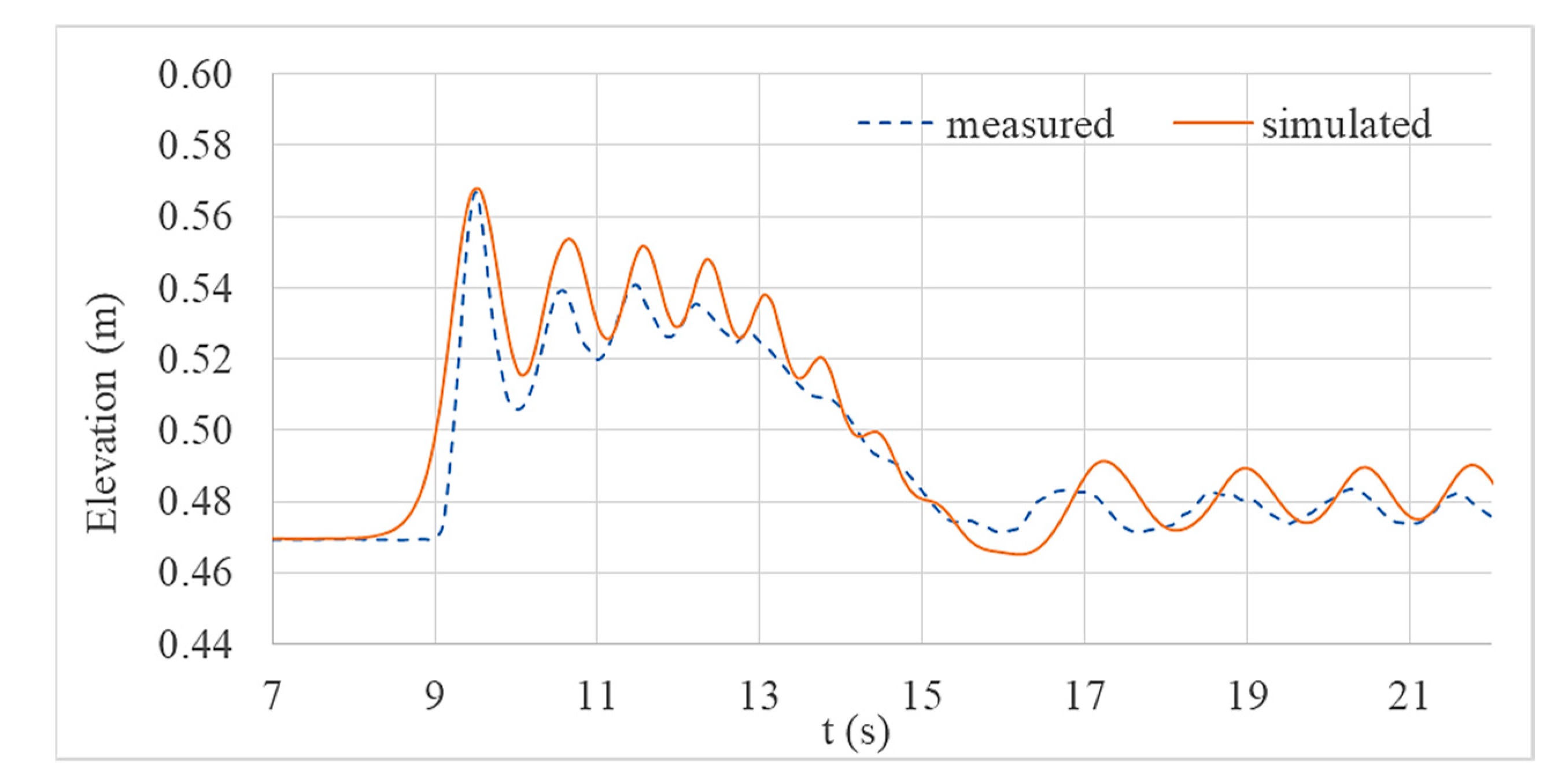
5. Validation of the Numerical Model

Although the numerical model was calibrated for an extent by water level and current velocity data, validation is necessary to justify the numerical results that are discussed under Section 4. However, we were unable to capture enough experimental data around the structure system due to some limitations of measuring instrumentation. Specially, current velocity variations at the structure system were could not be measured by our instrumentation as the structure was located above the still water level at the initial stage. Nevertheless, water level variations just in front of the wall and trench structure system (Location E in Figure 1) were measured for the simulation Case 03 (Table 2). The comparison of measured water level variations and simulation data are shown in Figure 28.

Although this comparison does not give much information from the view point of validation of flow around the structure, we think it can be considered for some extent. Furthermore, for the reader’s reference, validation of the OpenFOAM-interFOAM solver for dam break problems including structures are comprehensively done by Zhainakov and Kurbanaliev [24].

6. Conclusions

A set of experiments were carried out in a 2D wave flume to capture water level variations and current velocities at several locations.

A numerical model was then developed in OpenFOAM^® environment to replicate wave flume experiments. The numerical model was calibrated to acceptable limits to replicate water level variations and current velocities against experimental results. Though there were few deviations observed when comparing experimental and numerical results, the maximum free surface elevations and maximum current velocities were accurately reproduced by the numerical model.

The structure systems onshore were introduced into the numerical model. The consequence of a tsunami-like wave impacting a single wall and wall-trench systems were assessed and compared. All structures systems onshore resulted in depreciated water level variations at the lee side compared to cases without any defensive structures. This led to lower inundation lengths and lower run-up heights on a 1:100 slope.

The typical wall and trench system resulted lower water levels and lower current velocities at the lee side of the structure compared to a single wall. In addition, the combined structure delayed the wave bore for some extent once the overtopping wave interacted with the trench.

The wall and trench system was then numerically assessed by changing the geometrical properties of the structure. A 62.5 cm spacing between the wall and trench found to be the most effective in suppressing the striking wave. In this case, the overtopping wave crashed directly into the trench and produced higher turbulence in the trench. This behavior was further investigated by subjecting the structure system with different tsunami levels. Results indicated that the most effective reduction to the water levels and current velocities achievable was when the wave crashes directly in to the lee side trench. When the tsunami height was comparatively low, the critical spacing between the wall and the trench was also found out to be lower. Once the spacing between the wall -trench increases more than the critical spacing, the wave suppression has come into a threshold which still resulted in lower water level variations and current velocities at the land side when compared to those with a single seawall system.

The study found that the trench’s width also had a positive impact on wave suppression. The wider trenches resulted in better suppression of the wave. Similarly, wider walls lowered the water level variations and current velocities of a wave in a positive way and deeper trenches produced better depreciation of the waveform. Furthermore, by referring to the inundation comparisons, the reader can have a better idea and justification on the above discussed points.

When comparing the reduced water levels and current velocities, which were due to incorporating a trench to an existing embankment type single seawall. It was noticeable that the height of an existing or a planned seawall can be reduced by about 20%–30% achieving the same level of protection that would be expected by a single seawall.

Lastly, as the results of Section 4 suggests, it is conclusive that a combined wall and trench system onshore can effectively reduce an incoming tsunami-like wave. The reduction is comparatively better than that of the reduction, which occurs when an overtopping wave passes through a conventional single seawall system.

As the wall and trench system resulted in reducing both wave runup heights and current velocities at the lad side and increasing the tsunami arrival time when compared to a single seawall system. This study has clearly shown that it would be beneficial to consider these types of structure in future planning and implementing tsunami defense measures.

Nevertheless, the proposed structures can still suppress the striking tsunami-like wave for a certain extent and cannot provided a complete defense.

Most importantly, it should be highlighted that the performance of the wall and trench system presented in this study has not been comprehensively validated by an experimental study. Although the comparison of water level variations in front of the structure system were compared with simulated data, current velocity variations were not validated. Therefore, a validation study would be beneficial for the justification of the results presented in this article.

References

1. Goring, B.D.G.; Raichlen, F. Propagation of longwaves onto shelf. J. Waterw. Port Coast. Ocean Eng. 1992, 118, 43–61. [Google Scholar] [CrossRef]
2. Raby, A.; Macabuag, J.; Pomonis, A.; Wilkinson, S.; Rossetto, T. Implications of the 2011 Great East Japan Tsunami on sea defence design. Int. J. Disaster Risk Reduct. 2015, 14, 332–346. [Google Scholar] [CrossRef] [Green Version]
3. Synolakis, C.E.; Yalciner, A.C.; Imamura, F.; Fritz, H.M.; Suppasri, A.; Mas, E.; Kalligeris, N.; Necmioglu, O.; Ozer, C.; Zaytsev, A.; et al. Field survey of the coastal impact of the 11 March 2011 great East Japan tsunami. In Proceedings of the European Geosciences Union (EGU) General Assembly, Antalya, Turkey, 31 October–1 November 2011; p. 1. [Google Scholar]
4. Rahman, M.M.; Schaab, C.; Nakaza, E. Experimental and numerical modeling of tsunami mitigation by canals. J. Waterw. Port Coast. Ocean Eng. 2017, 143, 1–11. [Google Scholar] [CrossRef]
5. Kimura, S. When a seawall is visible: Infrastructure and obstruction in post-tsunami reconstruction in Japan. Sci. Cult. 2016, 25, 23–43. [Google Scholar] [CrossRef] [Green Version]
6. Hsiao, S.C.; Lin, T.C. Tsunami-like solitary waves impinging and overtopping an impermeable seawall: Experiment and RANS modeling. Coast. Eng. 2010, 57, 1–18. [Google Scholar] [CrossRef]
7. Esteban, M.; Glasbergen, T.; Takabatake, T.; Hofland, B.; Nishizaki, S.; Nishida, Y.; Stolle, J.; Nistor, I.; Bricker, J.; Takagi, H.; et al. Overtopping of coastal structures by tsunami waves. Geosciences 2017, 7, 121. [Google Scholar] [CrossRef] [Green Version]
8. Zaha, T.; Tanaka, N.; Kimiwada, Y. Flume experiments on optimal arrangement of hybrid defense system comprising an embankment, moat, and emergent vegetation to mitigate inundating tsunami current. Ocean Eng. 2019, 173, 45–57. [Google Scholar] [CrossRef]
9. Muhammad, R.A.H.; Tanaka, N. Energy reduction of a tsunami current through a hybrid defense system comprising a sea embankment followed by a coastal forest. Geosciences 2019, 9, 247. [Google Scholar] [CrossRef] [Green Version]
10. Rao, R.; Vijayaraghavan, B.; Sarma, S.; Satyanarayanan, M. Buckingham Canal saved people in Andhra Pradesh (India) from the tsunami of 26 December 2004. Curr. Sci. 2005, 89, 12–13. [Google Scholar]
11. Tokida, K.; Tanimoto, R. Lessons and views on hardware countermeasures with earth banks against tsunami estimated in 2011 Great East Japan Earthquake. In Proceedings of the International Symposium on Engineering Lessons Learned from the 2011 Great East Japan Earthquake, Tokyo, Japan, 1–4 March 2012; pp. 1–4. [Google Scholar]
12. Dao, N.X.; Adithyawan, M.B.; Tanaka, H. Sensitivity analysis of shore-parallel canal for tsunami wave energy reduction. J. Japan Soc. Civ. Eng. Ser. B3 Ocean Eng. 2013, 69, I_401–I_406. [Google Scholar] [CrossRef] [Green Version]
13. Silva, A.; Araki, S. Submerged wall-trench systems to suppress tsunami impact on coast. Proc. Int. Offshore Polar Eng. Conf. 2019, 3, 3253–3260. [Google Scholar]
14. NOWPHAS. Obseved Water Level Data of the Great East Japan Tsunami. Available online: https://nowphas.mlit.go.jp/pastdata/ (accessed on 5 January 2020).
15. Grilli, S.T.; Ioualalen, M.; Asavanant, J.; Shi, F.; Kirby, J.T.; Watts, P. Source constraints and model simulation of the December 26, 2004, Indian Ocean tsunami. J. Waterw. Port Coast Ocean. Eng. 2007, 133, 414–428. [Google Scholar] [CrossRef] [Green Version]
16. Damián, S.M.; Nigro, M.N. An extended mixture model for the simultaneous treatment of small-scale and large-scale interfaces. Inter. J. Numer. Methods Fluids 2014, 75, 547–574. [Google Scholar] [CrossRef]
17. Lopes, P.M.B. Free-Surface Flow Interface and Air-Entrainment Modelling Using OpenFOAM; Thesis Project in Hydraulic, Water Resources and Environment Doctoral Program in Civil Engineering; University of Coimbra: Coimbra, Portugal, 2013. [Google Scholar]
18. Jasak, H. Error Analysis and Estimation for Finite Volume Method with Applications to Fluid Flow; Imperial College of Science, Technology and Medicine: London, UK, 1996. [Google Scholar]
19. Ubbink, O. Numerical Prediction of Two Fluid Systems with Sharp Interfaces; University of London: Lodon, UK, 1997. [Google Scholar]
20. Rusche, H. Computational Dispersed Two-Phase Dynamics Flows of At Phase Fractions. Ph.D. Thesis, University of London, London, UK, 2003. [Google Scholar]
21. Deshpande, S.S.; Anumolu, L.; Trujillo, M.F. Evaluating the performance of the two-phase flow solver interFoam. Comput. Sci. Discov. 2012, 5, 014016. [Google Scholar] [CrossRef]
22. Cox, D.T.; Kobayashi, N.; Okayasu, A. Vertical variations of fluid velocities and shear stress in surf zones. Proc. Coast. Eng. Conf. 1995, 1, 98–112. [Google Scholar] [CrossRef]
23. Park, I.R.; Kim, K.S.; Kim, J.; Van, S.H. Numerical investigation of the effects of turbulence intensity on dam-break flows. Ocean. Eng. 2012, 42, 176–187. [Google Scholar] [CrossRef]
24. Zhainakov, A.Z.; Kurbanaliev, A.Y. Verification of the open package OpenFOAM on dam break problems. Thermophys. Aeromechanics 2013, 20, 451–461. [Google Scholar] [CrossRef]
Figure 1. Dimensions and other details of the experimental setup. Similar setup is applied in the numerical simulations which is described in the next section.
Geosciences 10 00310 g001
Figure 2. Geometry of the combined wall and trench system.
Geosciences 10 00310 g002
Figure 3. Geometry of the combined wall and trench system that is subjected to testing under Section 3.2.
Geosciences 10 00310 g003
Figure 4. Comparison of water level variations at location A.
Geosciences 10 00310 g004
Figure 5. Comparison of water level variations at location B.
Geosciences 10 00310 g005
Figure 6. Comparison of water level variations at location C.
Geosciences 10 00310 g006
Figure 7. Comparison of current velocity (x-component) at location B.
Geosciences 10 00310 g007
Figure 8. Comparison of current velocity (x-component) at location C.
Geosciences 10 00310 g008
Figure 9. Comparison of water level variations at location D.
Geosciences 10 00310 g009
Figure 10. Comparison of current velocity (x-component) variations at location D.
Geosciences 10 00310 g010
Figure 11. Comparison of water level variations at location D.
Geosciences 10 00310 g011
Figure 12. Comparison of current velocity (x-component) variations at location D.
Geosciences 10 00310 g012
Figure 13. Comparison of water level variations at location D.
Geosciences 10 00310 g013
Figure 14. Comparison of current velocity (x-component) variations at location D.
Geosciences 10 00310 g014
Figure 15. Comparison of water level variations at location D.
Geosciences 10 00310 g015
Figure 16. Comparison of current velocity (x-component) variations at location D.
Geosciences 10 00310 g016
Figure 17. Comparison of wave induced inundation for each simulation case with different spacings between wall and trench.
Geosciences 10 00310 g017
Figure 18. Comparison of wave run-up for each simulation case with different trench widths.
Geosciences 10 00310 g018
Figure 19. Comparison of wave run-up heights for each simulation case with different wall widths.
Geosciences 10 00310 g019
Figure 20. Comparison of wave run-up for each simulation case with different trench depths.
Geosciences 10 00310 g020
Figure 21. Comparison of maximum water levels observed at location D.
Geosciences 10 00310 g021
Figure 22. Comparison of maximum current velocity in x direction, observed at location D.
Geosciences 10 00310 g022
Figure 23. Comparison of maximum water levels observed at location D for different tsunami conditions.
Geosciences 10 00310 g023
Figure 24. Comparison of maximum current velocity in x direction, observed at location D for different tsunami conditions.
Geosciences 10 00310 g024
Figure 25. Current velocity vectors at t = 13.2 s for simulation Case 24 (Table 4).
Geosciences 10 00310 g025
Figure 26. Current velocity vectors at t = 13.2 s for simulation Case 36 (Table 4).
Geosciences 10 00310 g026
Figure 27. Current velocity vectors at t = 13.2 s for simulation Case 52 (Table 4).
Geosciences 10 00310 g027
Figure 28. Comparison of measured water level variations and simulated data at E.
Geosciences 10 00310 g028