Monitoring the Recent Activity of Landslides in the Mailuu-Suu Valley (Kyrgyzstan) Using Radar and Optical Remote Sensing Techniques


Abstract
1. Introduction
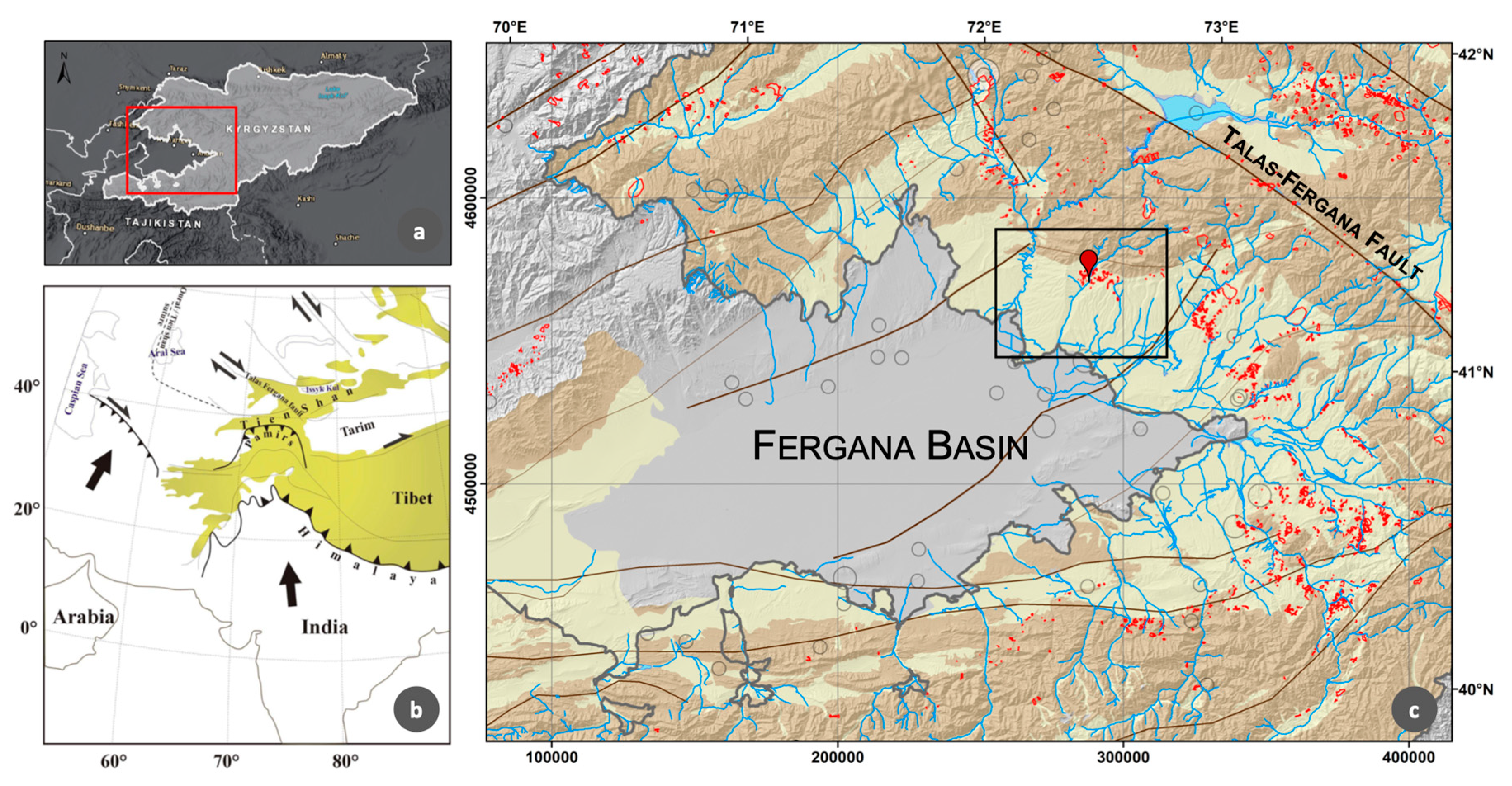
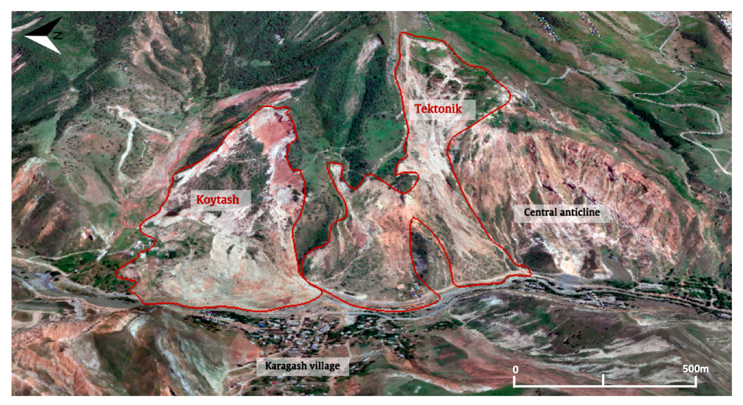
2. Study Area
3. Material and Methods
3.1. Comparison of Multitemporal Digital Elevation Models
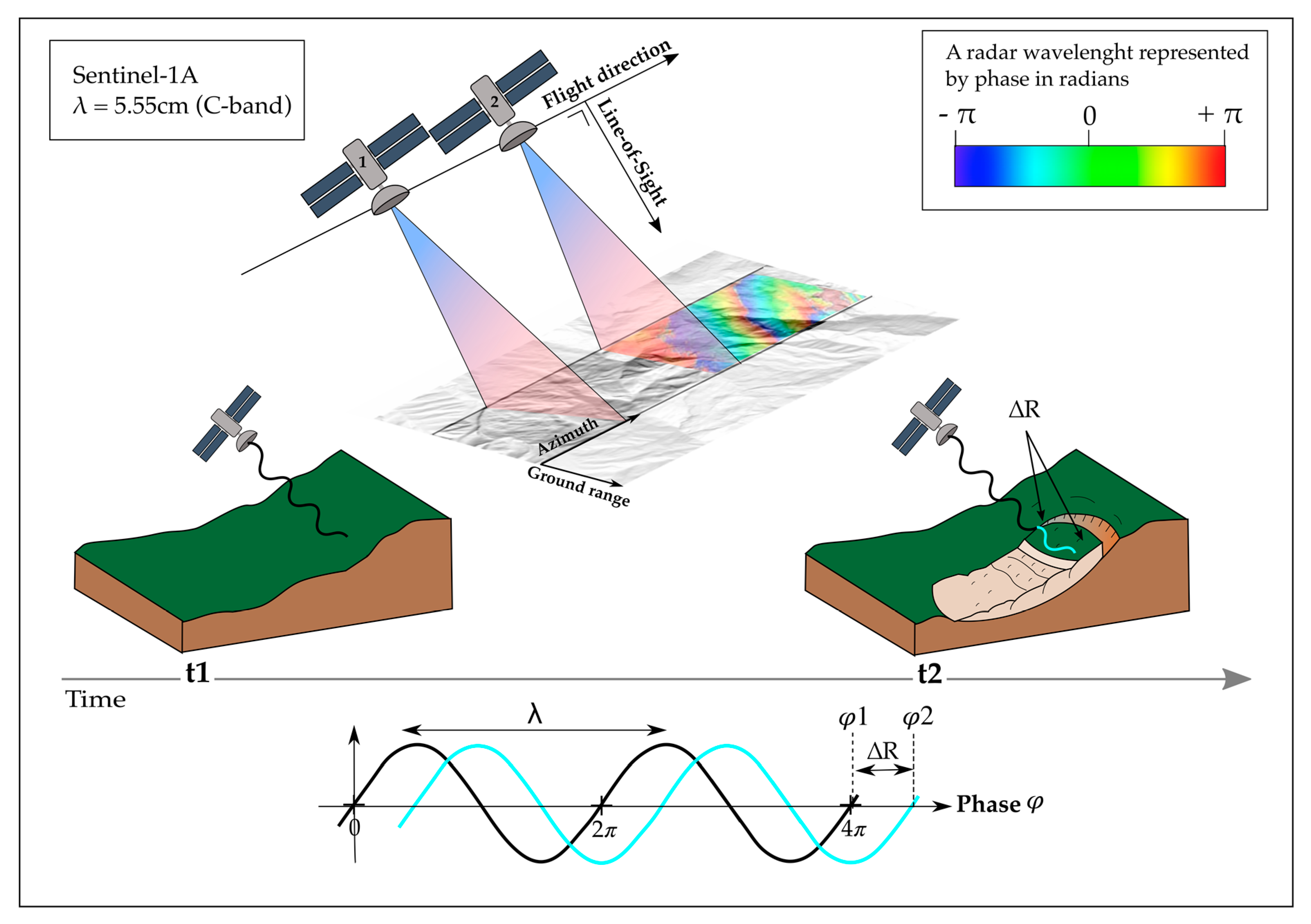
3.2. Radar Remote Sensing
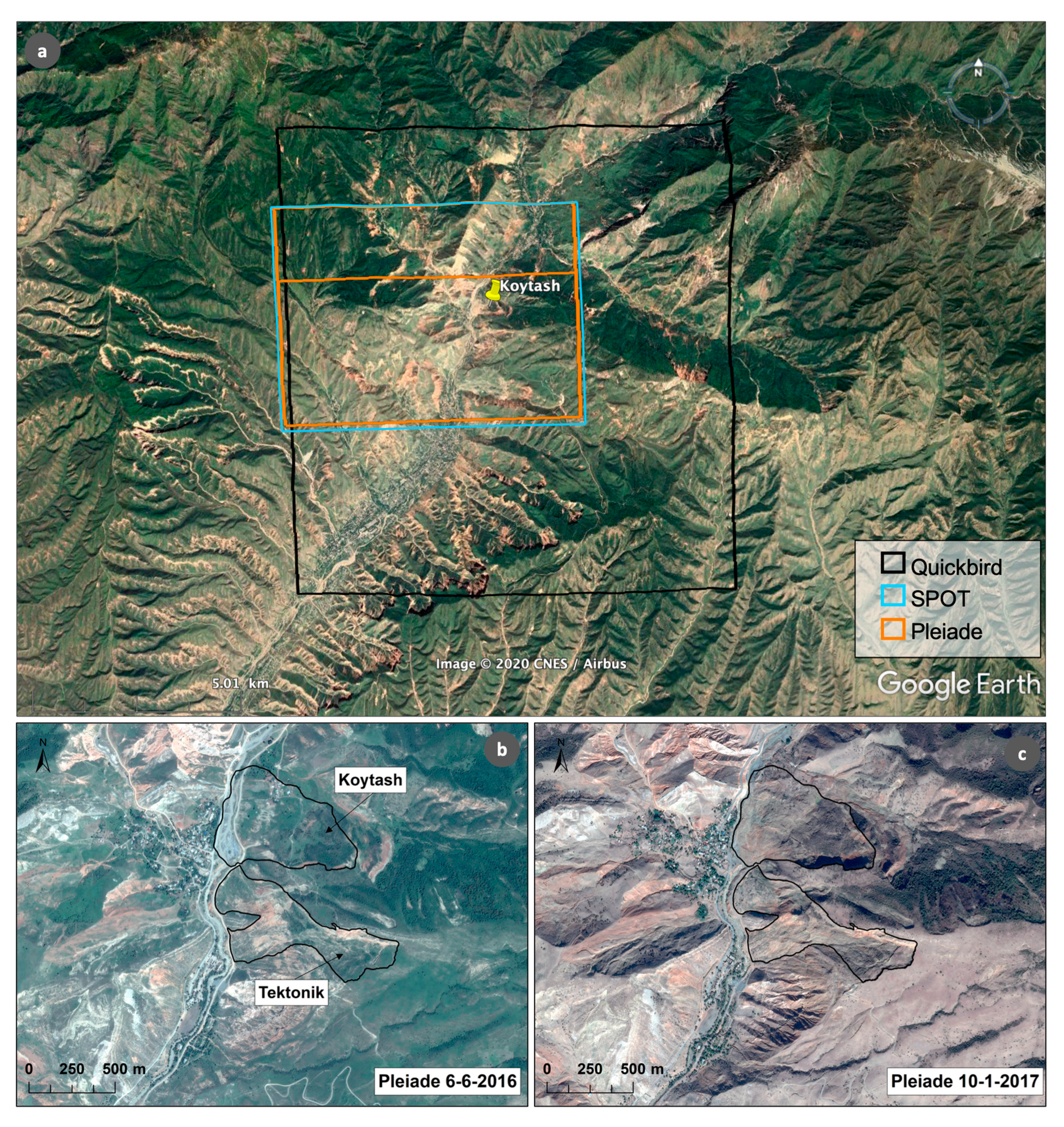
3.3. Optical Remote Sensing
3.4. Meteorological Data
4. Results
4.1. Differences between Pre- and Post-Failure Topography
4.2. Landslide Displacements from D-InSAR Analysis
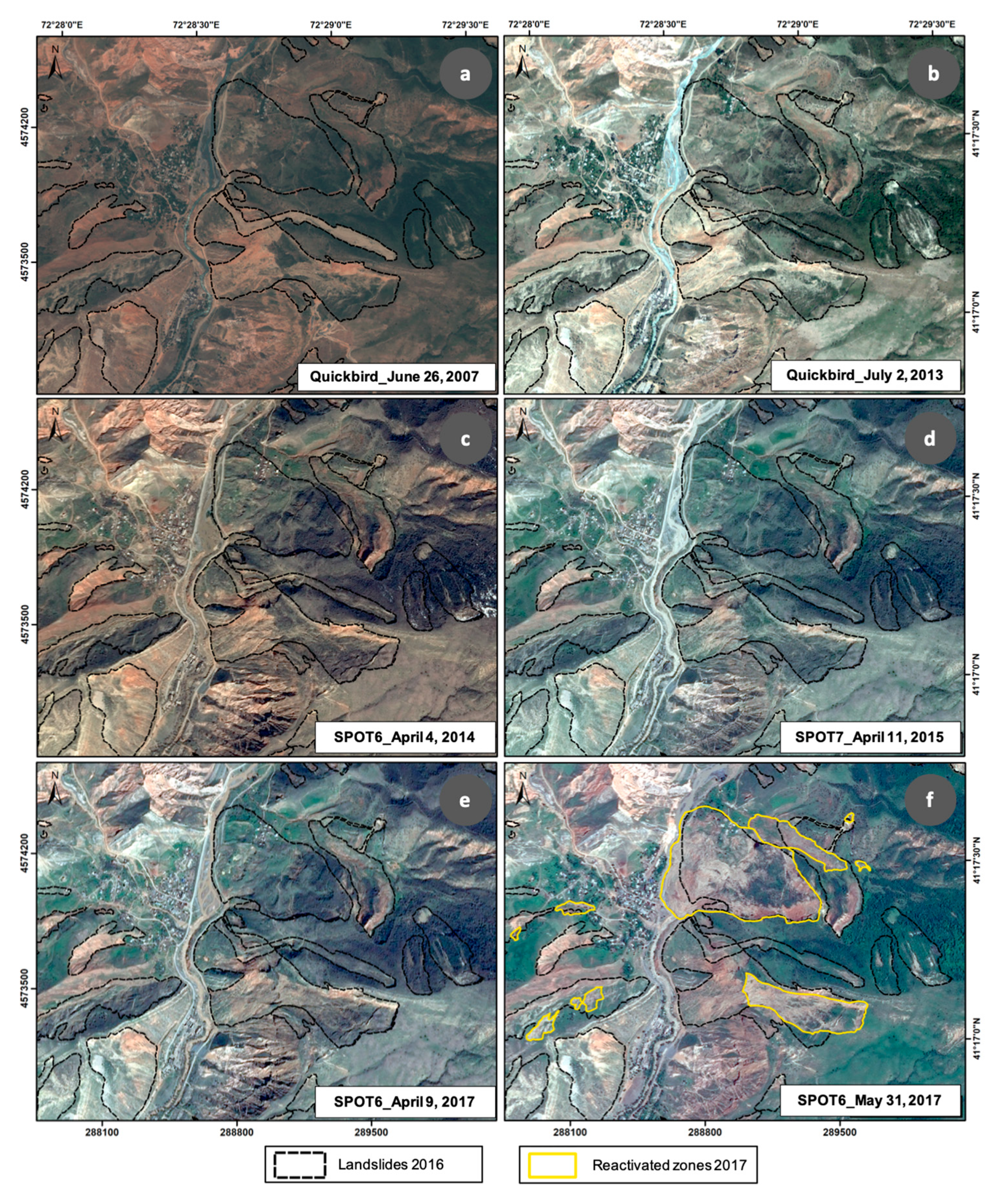
4.3. Mapping of Reactivated Zones and NDVI Analysis
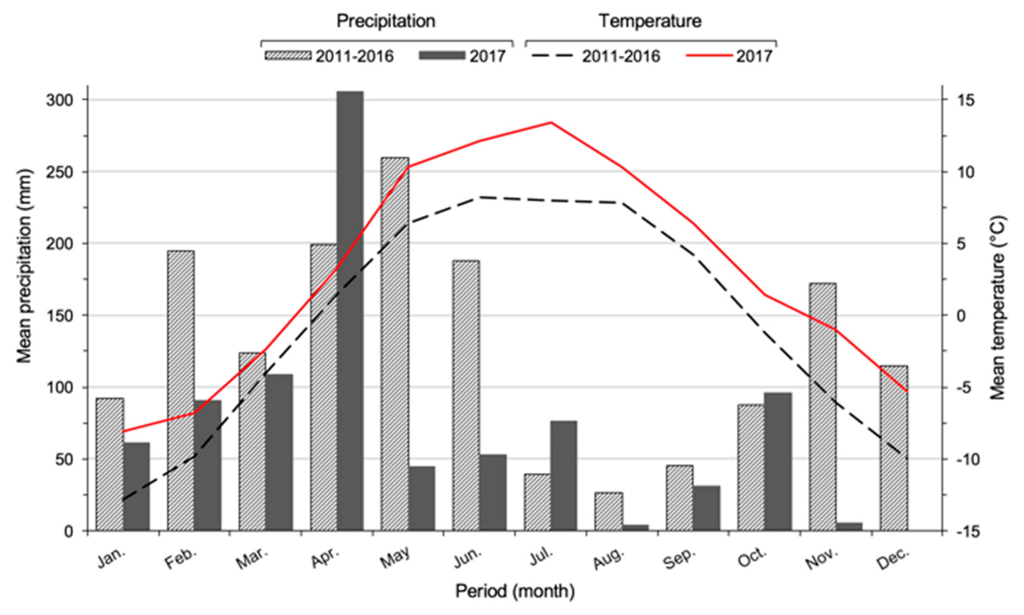
4.4. Identification of the Meteorological Triggering Factors
5. Discussion
6. Conclusions
Author Contributions
Funding
Acknowledgments
Conflicts of Interest
Appendix A


| Ground Control Points (GCPs) | 11 | 13 | 23 | 24 | Δ Mean DGPS-DEM |
|---|---|---|---|---|---|
| Longitude Latitude (DD) | 72.483867 41.282283 | 72.479250 41.293169 | 72.476339 41.285775 | 72.476217 41.284550 | |
| DGPS altitude (m) | 1271.50 | 1018.50 | 982.60 | 957.10 | |
| SRTM alt (m) | 1305.87 | 1056.50 | 1020.21 | 990.92 | |
| ΔDGPS–SRTM (m) | −34.37 | −38.00 | −37.61 | −33.82 | −35.95 |
| SPOT alt (m) | 1292.00 | 1050.00 | 994.00 | 987.00 | |
| ΔDGPS–SPOT (m) | −20.50 | −31.50 | −11.40 | −29.90 | −23.33 |
| ASTER alt (m) | 1301.46 | 1050.83 | 1008.95 | 986.63 | |
| ΔDGPS–ASTER (m) | −29.96 | −32.33 | −26.35 | −29.53 | −29.54 |
| TanDEM-X alt (m) | 1265.88 | 1013.79 | 981.95 | 949.87 | |
| ΔDGPS–TanDEM-X (m) | 5.62 | 4.71 | 0.65 | 7.23 | 4.55 |
References
- Klein, J.A.; Tucker, C.M.; Steger, C.E.; Nolin, A.; Reid, R.; Hopping, K.A.; Yeh, E.T.; Pradhan, M.S.; Taber, A.; Molden, D.; et al. An Integrated Community and Ecosystem-Based Approach to Disaster Risk Reduction in Mountain Systems. Environ. Sci. Policy 2019, 94, 143–152. [Google Scholar] [CrossRef]
- Zhao, C.; Lu, Z. Remote Sensing of Landslides—A Review. Remote Sens. 2018, 10, 279. [Google Scholar] [CrossRef]
- Saponaro, A.; Pilz, M.; Bindi, D.; Parolai, S. The Contribution of EMCA to Landslide Susceptibility Mapping in Central Asia. Ann. Geophys. 2015, 58. [Google Scholar] [CrossRef]
- Roessner, S.; Wetzel, H.U.; Kaufmann, H.; Sarnagoev, A. Potential of Satellite Remote Sensing and GIS for Landslide Hazard Assessment in Southern Kyrgyzstan (Central Asia). Nat. Hazards 2005, 35, 395–416. [Google Scholar] [CrossRef]
- Havenith, H.B.; Torgoev, I.; Meleshko, A.; Alioshin, Y.; Torgoev, A.; Danneels, G. Landslides in the Mailuu-Suu Valley, Kyrgyzstan - Hazards and Impacts. Landslides 2006, 3, 137–147. [Google Scholar] [CrossRef]
- Havenith, H.-B.B.; Umaraliev, R.; Schlögel, R.; Torgoev, I.; Ruslan, U.; Schlogel, R.; Torgoev, I. Past and Potential Future Socioeconomic Impacts of Environmental Hazards in Kyrgyzstan. In Kyrgyzstan: Political, Economic and Social Issues; Olivier, A.P., Ed.; Nova Science Publishers, Inc.: Hauppauge, NY, USA, 2017; pp. 63–113. [Google Scholar]
- Behling, R.; Roessner, S. Spatiotemporal Landslide Mapper for Large Areas Using Optical Satellite Time Series Data. In Advancing Culture of Living with Landslides; Sassa, K., Mikoš, M., Yin, Y., Eds.; Springer International Publishing: Cham, Switzerland, 2017; pp. 143–152. [Google Scholar]
- Lu, Z.; Dzurisin, D. InSAR Imaging of Aleutian Volcanoes; Springer: Berlin/Heidelberg, Germany, 2014. [Google Scholar]
- Massonnet, D.; Feigl, K.L. Radar Interferometry and Its Application to Changes in the Earth’s Surface. Rev. Geophys. 1998, 36, 441–500. [Google Scholar] [CrossRef]
- Ouchi, K. Recent Trend and Advance of Synthetic Aperture Radar with Selected Topics. Remote Sens. 2013, 5, 716–807. [Google Scholar] [CrossRef]
- Schlögel, R.; Doubre, C.; Malet, J.P.; Masson, F. Landslide Deformation Monitoring with ALOS/PALSAR Imagery: A D-InSAR Geomorphological Interpretation Method. Geomorphology 2015, 231, 314–330. [Google Scholar] [CrossRef]
- Teshebaeva, K.; Roessner, S.; Echtler, H.; Motagh, M.; Wetzel, H.U.; Molodbekov, B. ALOS/PALSAR InSAR Time-Series Analysis for Detecting Very Slow-Moving Landslides in Southern Kyrgyzstan. Remote Sens. 2015, 7, 8973–8994. [Google Scholar] [CrossRef]
- Wauthier, C. InSAR Applied to the Study of Active Volcanic and Seismic Areas in Africa. Ph.D. Thesis, Université de Liège, Liège, Belgium, 2011. [Google Scholar]
- Peyret, M.; Djamour, Y.; Rizza, M.; Ritz, J.-F.; Hurtrez, J.-E.; Goudarzi, M.A.; Nankali, H.; Chéry, J.; Le Dortz, K.; Uri, F. Monitoring of the Large Slow Kahrod Landslide in Alborz Mountain Range (Iran) by GPS and SAR Interferometry. Eng. Geol. 2008, 100, 131–141. [Google Scholar] [CrossRef]
- Handwerger, A.L.; Roering, J.J.; Schmidt, D.A. Controls on the Seasonal Deformation of Slow-Moving Landslides. Earth Planet. Sci. Lett. 2013, 377–378, 239–247. [Google Scholar] [CrossRef]
- Colesanti, C.; Wasowski, J. Investigating Landslides with Space-Borne Synthetic Aperture Radar (SAR) Interferometry. Eng. Geol. 2006, 88, 173–199. [Google Scholar] [CrossRef]
- Jebur, M.N.; Pradhan, B.; Tehrany, M.S. Detection of Vertical Slope Movement in Highly Vegetated Tropical Area of Gunung Pass Landslide, Malaysia, Using L-Band InSAR Technique. Geosci. J. 2014, 18, 61–68. [Google Scholar] [CrossRef]
- Dai, K.; Li, Z.; Tomás, R.; Liu, G.; Yu, B.; Wang, X.; Cheng, H.; Chen, J.; Stockamp, J. Monitoring Activity at the Daguangbao Mega-Landslide (China) Using Sentinel-1 TOPS Time Series Interferometry. Remote Sens. Environ. 2016, 186, 501–513. [Google Scholar] [CrossRef]
- Behling, R.; Roessner, S.; Kaufmann, H.; Kleinschmit, B. Automated Spatiotemporal Landslide Mapping over Large Areas Using Rapideye Time Series Data. Remote Sens. 2014, 6, 8026–8055. [Google Scholar] [CrossRef]
- Hölbling, D.; Friedl, B.; Eisank, C. An Object-Based Approach for Semi-Automated Landslide Change Detection and Attribution of Changes to Landslide Classes in Northern Taiwan. Earth Sci. Informatics 2015, 8, 327–335. [Google Scholar] [CrossRef]
- Stumpf, A.; Malet, J.P.; Allemand, P.; Ulrich, P. Surface Reconstruction and Landslide Displacement Measurements with Pléiades Satellite Images. ISPRS J. Photogramm. Remote Sens. 2014, 95, 1–12. [Google Scholar] [CrossRef]
- Zylshal; Sulma, S.; Yulianto, F.; Nugroho, J.T.; Sofan, P. A Support Vector Machine Object Based Image Analysis Approach on Urban Green Space Extraction Using Pleiades-1A Imagery. Model. Earth Syst. Environ. 2016, 2, 1–12. [Google Scholar] [CrossRef]
- Schlogel, R.; Torgoev, I.; De Marneffe, C.; Havenith, H.B. Evidence of a Changing Size-Frequency Distribution of Landslides in the Kyrgyz Tien Shan, Central Asia. Earth Surf. Process. Landf. 2011, 36, 1658–1669. [Google Scholar] [CrossRef]
- Behling, R.; Roessner, S.; Golovko, D.; Kleinschmit, B. Derivation of Long-Term Spatiotemporal Landslide Activity—A Multi-Sensor Time Series Approach. Remote Sens. Environ. 2016, 186, 88–104. [Google Scholar] [CrossRef]
- Li, Z.; Shi, W.; Myint, S.W.; Lu, P.; Wang, Q. Semi-Automated Landslide Inventory Mapping from Bitemporal Aerial Photographs Using Change Detection and Level Set Method. Remote Sens. Environ. 2016, 175, 215–230. [Google Scholar] [CrossRef]
- Havenith, H.B.; Jongmans, D.; Faccioli, E.; Abdrakhmatov, K.; Bard, P.Y. Site Effect Analysis around the Seismically Induced Ananevo Rockslide, Kyrgyzstan. Bull. Seismol. Soc. Am. 2002. [Google Scholar] [CrossRef]
- Havenith, H.B.; Torgoev, A.; Schlögel, R.; Braun, A.; Torgoev, I.; Ischuk, A. Tien Shan Geohazards Database: Landslide Susceptibility Analysis. Geomorphology 2015, 249, 32–43. [Google Scholar] [CrossRef]
- Haberland, C.; Abdybachaev, U.; Schurr, B.; Wetzel, H.U.; Roessner, S.; Sarnagoev, A.; Orunbaev, S.; Janssen, C. Landslides in Southern Kyrgyzstan: Understanding Tectonic Controls. Eos 2011, 92, 169–170. [Google Scholar] [CrossRef]
- Torgoev, I.; Aleshyn, U.; Havenith, H. Impact of Uranium Mining and Processing on the Environment of Mountainous Areas of Kyrgyzstan. In Uranium in the Aquatic Environment; Merkel, B.J., Planer-Friedrich, B., Wolkersdorfer, C., Eds.; Springer Berlin Heidelberg: New York, NY, USA, 2002; pp. 1–6. [Google Scholar]
- Vandenhove, H.; Quarch, H.; Sweeck, L.; Sillen, X.; Mallants, D. Remediation of Uranium Mining and Milling Tailing in Mailuu-Suu District of Kyrgyzstan; Tacis Project N° SCRE1/N°38; SCK CEN: Mol, Belgium, 2003. [Google Scholar]
- Saponaro, A.; Pilz, M.; Wieland, M.; Bindi, D.; Moldobekov, B.; Parolai, S. Landslide Susceptibility Analysis in Data-Scarce Regions: The Case of Kyrgyzstan. Bull. Eng. Geol. Environ. 2015, 74, 1117–1136. [Google Scholar] [CrossRef]
- Lollino, G.; Giordan, D.; Crosta, G.B.; Corominas, J.; Azzam, R.; Wasowski, J.; Sciarra, N. Engineering Geology for Society and Territory—Volume 2: Landslide Processes; Springer: Berlin, Germany, 2015; Volume 2, pp. 1–2177. [Google Scholar]
- Torgoev, I.; Abdrakhmatov, K.; Kasymbek, S.U.; Strom, A.L.; Kristekova, M.; Havenith, H.; Korup, O. Prevention of Landslide Dam Disasters in the Tien Shan, Kyrgyz Republic; NATO: Brussels, Belgium, 2012. [Google Scholar]
- Torgoev, I.A.; Aleshin, Y.G.; Meleshko, A.V.; Havenith, H.B. Hazard Mitigation for Landslide Dams in Mailuu-Suu Valley (Kyrgyzstan). Ital. J. Eng. Geol. Environ. 2006, 99–102. [Google Scholar]
- Danneels, G.; Bourdeau, C.; Torgoev, I.; Havenith, H.B. Geophysical Investigation and Dynamic Modelling of Unstable Slopes: Case-Study of Kainama (Kyrgyzstan). Geophys. J. Int. 2008, 175, 17–34. [Google Scholar] [CrossRef]
- Havenith, H.-B. Landslides Triggered by Earthquakes—Experimental Studies in the Tien Shan Mountains (Central Asia) and Dynamic Modelling. Ph.D. Thesis, University of Liège, Liège, Belgium, 2002. [Google Scholar]
- Schlögel, R. Detection of Recent Landslides in Maily-Say Valley, Kyrgyz Tien Shan, Based on Field Observations and Remote Sensing Data. Master’s Thesis, University of Liège, Liège, Belgium, 2009. [Google Scholar]
- Torgoev, I. Personal Communication; GEOPRIBOR-Scientific Engineering Center: Bishkek, Kyrgyzstan, 2017. [Google Scholar]
- Giorgio, H.-Ö.; Markus, K.; Wolfhart, P.; Nedim, R. The “Tektonik” Landslide at Mailuu Suu, Kyrgyz Republic. In Engineering Geology for Society and Territory—Volume 2; Springer International Publishing: Cham, Switherland, 2015; Volume 2, pp. 1055–1059. [Google Scholar]
- Abdrakhmatov, K.; Havenith, H.B.; Delvaux, D.; Jongmans, D.; Trefois, P. Probabilistic PGA and Arias Intensity Maps of Kyrgyzstan (Central Asia). J. Seismol. 2003. [Google Scholar] [CrossRef]
- Torgoev, A.; Havenith, H.B. 2D Dynamic Studies Combined with the Surface Curvature Analysis to Predict Arias Intensity Amplification. J. Seismol. 2016, 20, 711–731. [Google Scholar] [CrossRef]
- Torgoev, I.; Niyazov, R.; Havenith, H.-B. Tien-Shan Landslides Triggered by Earthquakes in Pamir-Hindukush Zone. In Landslide Science and Practice; Margottini, C., Canuti, P., Sassa, K., Eds.; Springer: Berlin/Heidelberg, Germany, 2013; pp. 191–197. [Google Scholar]
- Jaud, M.; Passot, S.; Le Bivic, R.; Delacourt, C.; Grandjean, P.; Le Dantec, N. Assessing the Accuracy of High Resolution Digital Surface Models Computed by PhotoScan® and MicMac® in Sub-Optimal Survey Conditions. Remote Sens. 2016, 8, 465. [Google Scholar] [CrossRef]
- Bardi, F.; Frodella, W.; Ciampalini, A.; Bianchini, S.; Del Ventisette, C.; Gigli, G.; Fanti, R.; Moretti, S.; Basile, G.; Casagli, N. Integration between Ground Based and Satellite SAR Data in Landslide Mapping: The San Fratello Case Study. Geomorphology 2014, 223, 45–60. [Google Scholar] [CrossRef]
- Bamler, R.; Hartl, P. Synthetic Aperture Radar Interferometry. Inverse Probl. 1998, 14, 1–54. [Google Scholar] [CrossRef]
- Torres, R.; Snoeij, P.; Geudtner, D.; Bibby, D.; Davidson, M.; Attema, E.; Potin, P.; Rommen, B.Ö.; Floury, N.; Brown, M.; et al. GMES Sentinel-1 Mission. Remote Sens. Environ. 2012, 120, 9–24. [Google Scholar] [CrossRef]
- Interferometric Synthetic Aperture Radar—Geoscience Australia. Available online: https://www.ga.gov.au/scientific-topics/positioning-navigation/geodesy/geodetic-techniques/interferometric-synthetic-aperture-radar (accessed on 16 March 2020).
- Pepe, A.; Calò, F. A Review of Interferometric Synthetic Aperture RADAR (InSAR) Multi-Track Approaches for the Retrieval of Earth’s Surface Displacements. Appl. Sci. 2017, 7, 1264. [Google Scholar] [CrossRef]
- Samsonov, S.; Dille, A.; Dewitte, O.; Kervyn, F.; D’Oreye, N. Satellite Interferometry for Mapping Surface Deformation Time Series in One, Two and Three Dimensions: A New Method Illustrated on a Slow-Moving Landslide. Eng. Geol. 2020, 266, 105471. [Google Scholar] [CrossRef]
- Nobile, A.; Dille, A.; Monsieurs, E.; Basimike, J.; Bibentyo, T.; D’Oreye, N.; Kervyn, F.; Dewitte, O. Multi-Temporal DInSAR to Characterise Landslide Ground Deformations in a Tropical Urban Environment: Focus on Bukavu (DR Congo). Remote Sens. 2018, 10, 626. [Google Scholar] [CrossRef]
- Tiwari, A.; Narayan, A.B.; Dwivedi, R.; Dikshit, O.; Nagarajan, B. Monitoring of Landslide Activity at the Sirobagarh Landslide, Uttarakhand, India, Using LiDAR, SAR Interferometry and Geodetic Surveys. Geocarto Int. 2020, 35, 535–558. [Google Scholar] [CrossRef]
- Barra, A.; Solari, L.; Béjar-Pizarro, M.; Monserrat, O.; Bianchini, S.; Herrera, G.; Crosetto, M.; Sarro, R.; González-Alonso, E.; Mateos, R.; et al. A Methodology to Detect and Update Active Deformation Areas Based on Sentinel-1 SAR Images. Remote Sens. 2017, 9, 1002. [Google Scholar] [CrossRef]
- Imamoglu, M.; Kahraman, F.; Cakir, Z.; Sanli, F.B. Ground Deformation Analysis of Bolvadin (W. Turkey) by Means of Multi-Temporal InSAR Techniques and Sentinel-1 Data. Remote Sens. 2019, 11, 1069. [Google Scholar] [CrossRef]
- Yang, B.; Xu, H.; Liu, W.; Ge, J.; Li, C.; Li, J. An Improved Stanford Method for Persistent Scatterers Applied to 3D Building Reconstruction and Monitoring. Remote Sens. 2019, 11, 1807. [Google Scholar] [CrossRef]
- Czikhardt, R.; Papco, J.; Bakon, M.; Liscak, P.; Ondrejka, P.; Zlocha, M. Ground Stability Monitoring of Undermined and Landslide Prone Areas by Means of Sentinel-1 Multi-Temporal InSAR, Case Study from Slovakia. Geosciences 2017, 7, 87. [Google Scholar] [CrossRef]
- Derauw, D. Phasimétrie Par Radar à Synthèse d’Ouverture; Théorie et Applications. Ph.D. Thesis, Université de Liège, Liège, Belgium, 1999. [Google Scholar]
- Galve, J.P.; Pérez-Peña, J.V.; Azañón, J.M.; Closson, D.; Caló, F.; Reyes-Carmona, C.; Jabaloy, A.; Ruano, P.; Mateos, R.M.; Notti, D.; et al. Evaluation of the SBAS InSAR Service of the European Space Agency’s Geohazard Exploitation Platform (GEP). Remote Sens. 2017, 9, 1291. [Google Scholar] [CrossRef]
- Geohazards-TEP. Available online: https://geohazards-tep.eu/ (accessed on 30 April 2020).
- Schlögel, R.; Kofler, C.; Gariano, S.L.; Van Campenhout, J.; Plummer, S. Changes in Climate Patterns and Their Association to Natural Hazard Distribution in South Tyrol (Eastern Italian Alps). Sci. Rep. 2020, 10, 5022. [Google Scholar] [CrossRef] [PubMed]
- FASTVEL for Displacement Velocity Map Generation. Available online: https://terradue.github.io/doc-tep-geohazards/tutorials/fastvel.html (accessed on 16 April 2020).
- Stumpf, A.; Malet, J.-P.; Puissant, A.; Travelletti, J. Monitoring of Earth Surface Motion and Geomorphologic Processes by Optical Image Correlation. In Land Surface Remote Sensing; ISTE Press –Elsevier: London, UK, 2016; pp. 147–190. [Google Scholar]
- Wasowski, J.; Bovenga, F. Investigating Landslides and Unstable Slopes with Satellite Multi Temporal Interferometry: Current Issues and Future Perspectives. Eng. Geol. 2014, 174, 103–138. [Google Scholar] [CrossRef]
- Li, Z.; Shi, W.; Lu, P.; Yan, L.; Wang, Q.; Miao, Z. Landslide Mapping from Aerial Photographs Using Change Detection-Based Markov Random Field. Remote Sens. Environ. 2016, 187, 76–90. [Google Scholar] [CrossRef]
- Lillesand, T.M.; Kiefer, R.W.; Chipman, J.W. Remote Sensing and Image Interpretation, 6th ed.; John Wiley & Sons: Hoboken, NJ, USA, 2008. [Google Scholar]
- Pettorelli, N. NDVI from A to Z. In The Normalized Difference Vegetation Index; Oxford University Press: Oxford, UK, 2013; pp. 30–43. [Google Scholar]
- Monsieurs, E.; Dewitte, O.; Demoulin, A. A Susceptibility-Based Rainfall Threshold Approach for Landslide Occurrence. Nat. Hazards Earth Syst. Sci. 2019, 19, 775–789. [Google Scholar] [CrossRef]
- Schlögel, R.; Malet, J.P.; Doubre, C.; Lebourg, T. Structural Control on the Kinematics of the Deep-Seated La Clapière Landslide Revealed by L-Band InSAR Observations. Landslides 2016, 13, 1005–1018. [Google Scholar] [CrossRef]
- Fuhrmann, T.; Garthwaite, M.C. Resolving Three-Dimensional Surface Motion with InSAR: Constraints from Multi-Geometry Data Fusion. Remote Sens. 2019, 11, 241. [Google Scholar] [CrossRef]
- Sun, L.; Muller, J.P.; Chen, J. Time Series Analysis of Very Slow Landslides in the Three Gorges Region through Small Baseline SAR Offset Tracking. Remote Sens. 2017, 9, 1314. [Google Scholar] [CrossRef]
- Hu, B.; Wang, H.S.; Sun, Y.L.; Hou, J.G.; Liang, J. Long-Term Land Subsidence Monitoring of Beijing (China) Using the Small Baseline Subset (SBAS) Technique. Remote Sens. 2014, 6, 3648–3661. [Google Scholar] [CrossRef]
- Tofani, V.; Raspini, F.; Catani, F.; Casagli, N. Persistent Scatterer Interferometry (Psi) Technique for Landslide Characterization and Monitoring. Remote Sens. 2013, 5, 1045–1065. [Google Scholar] [CrossRef]
- Zhao, C.; Zhang, Q.; He, Y.; Peng, J.; Yang, C.; Kang, Y. Small-Scale Loess Landslide Monitoring with Small Baseline Subsets Interferometric Synthetic Aperture Radar Technique—Case Study of Xingyuan Landslide, Shaanxi, China. J. Appl. Remote Sens. 2016, 10, 026030. [Google Scholar] [CrossRef]
- Schlögel, R. Quantitative Landslide Hazard Assessment with Remote Sensing Observations and Statistical Modelling. Ph.D. Thesis, University of Strasbourg, Strasbourg, France, 2015. [Google Scholar]
- Fan, J.R.; Zhang, X.Y.; Su, F.H.; Ge, Y.G.; Tarolli, P.; Yang, Z.Y.; Zeng, Z. Geometrical Feature Analysis and Disaster Assessment of the Xinmo Landslide Based on Remote Sensing Data. J. Mt. Sci. 2017, 14, 1677–1688. [Google Scholar] [CrossRef]
- Fan, X.; Zhan, W.; Dong, X.; van Westen, C.; Xu, Q.; Dai, L.; Yang, Q.; Huang, R.; Havenith, H.B. Analyzing Successive Landslide Dam Formation by Different Triggering Mechanisms: The Case of the Tangjiawan Landslide, Sichuan, China. Eng. Geol. 2018, 243, 128–144. [Google Scholar] [CrossRef]
- Schlögel, R.; Braun, A.; Torgoev, A.; Fernandez-Steeger, T.M.; Havenith, H.B.; Schlögel, R.; Braun, A.; Torgoev, A.; Fernandez-Steeger, T.M.; Havenith, H.B. Assessment of Landslides Activity in Maily-Say Valley, Kyrgyz Tien Shan. In Landslide Science and Practice: Landslide Inventory and Susceptibility and Hazard Zoning; Springer: Berlin, Germany, 2011. [Google Scholar]
- Golovko, D.; Roessner, S.; Behling, R.; Wetzel, H.U.; Kleinschmit, B. Evaluation of Remote-Sensing-Based Landslide Inventories for Hazard Assessment in Southern Kyrgyzstan. Remote Sens. 2017, 9, 943. [Google Scholar] [CrossRef]
- Sassa, K.; Canuti, P.; Yin, Y.; Studies, L. Landslide Science for a Safer Geoenvironment: Volume 3: Targeted Landslides; Springer International Publishing: Cham, Switzerland, 2014; Volume 3. [Google Scholar]
- Schulz, W.H.; Coe, J.A.; Ricci, P.P.; Smoczyk, G.M.; Shurtleff, B.L.; Panosky, J. Landslide Kinematics and Their Potential Controls from Hourly to Decadal Timescales: Insights from Integrating Ground-Based InSAR Measurements with Structural Maps and Long-Term Monitoring Data. Geomorphology 2017, 285, 121–136. [Google Scholar] [CrossRef]


| DEM | Date | Spatial Resolution | Coordinates System | Vertical Datum | Source |
|---|---|---|---|---|---|
| SRTM | 2000 | 30 m (1 arc-second) | WGS84 | EGM96 | Shuttle Radar Topography Mission NASA |
| SPOT | 1 April 2006 | 20 m | WGS84 | EGM96 | Airbus Defence and Space |
| ASTER | 16 March 2011 | 30 m (1 arc-second) | WGS84 | EGM96 | NASA |
| TanDEM-X | 14 March 2011 | 12 m | WGS84 | WGS84 | WorldDEM, DLR & Airbus Defence and Space |
| UAV | 15 August 2017 | 0.2 m | WGS84 | - | Georisk Laboratory, ULiège |
| Sentinel-1A | Properties |
|---|---|
| Microwave band (wavelength) | C-band (5.55 cm) |
| Imaging mode | TOPSAR |
| Orbital geometry | Ascending |
| Acquisition mode | IW |
| Spatial resolution | 5 m × 20 m |
| Acquisition date | From 23 January 2016 to 31 December 2017 |
| Incidence angle | 29.1° to 46° |
| Type | SLC |
| Treatment level | 1 |
| Polarization | VV |
© 2020 by the authors. Licensee MDPI, Basel, Switzerland. This article is an open access article distributed under the terms and conditions of the Creative Commons Attribution (CC BY) license (http://creativecommons.org/licenses/by/4.0/).
Share and Cite
Piroton, V.; Schlögel, R.; Barbier, C.; Havenith, H.-B. Monitoring the Recent Activity of Landslides in the Mailuu-Suu Valley (Kyrgyzstan) Using Radar and Optical Remote Sensing Techniques. Geosciences 2020, 10, 164. https://doi.org/10.3390/geosciences10050164
Piroton V, Schlögel R, Barbier C, Havenith H-B. Monitoring the Recent Activity of Landslides in the Mailuu-Suu Valley (Kyrgyzstan) Using Radar and Optical Remote Sensing Techniques. Geosciences. 2020; 10(5):164. https://doi.org/10.3390/geosciences10050164
Chicago/Turabian StylePiroton, Valentine, Romy Schlögel, Christian Barbier, and Hans-Balder Havenith. 2020. "Monitoring the Recent Activity of Landslides in the Mailuu-Suu Valley (Kyrgyzstan) Using Radar and Optical Remote Sensing Techniques" Geosciences 10, no. 5: 164. https://doi.org/10.3390/geosciences10050164
APA StylePiroton, V., Schlögel, R., Barbier, C., & Havenith, H.-B. (2020). Monitoring the Recent Activity of Landslides in the Mailuu-Suu Valley (Kyrgyzstan) Using Radar and Optical Remote Sensing Techniques. Geosciences, 10(5), 164. https://doi.org/10.3390/geosciences10050164