Abstract
The rock slope stability assessment can be performed by means of deterministic and probabilistic approaches. As the deterministic analysis needs only representative values (generally, the mean value) for each physical and geo-mechanical parameter involved, it does not take into account the variability and uncertainty of geo-structural and geo-mechanical properties of joints. This analysis can be usually carried out using different methods, such as the Limit Equilibrium method or numerical modeling techniques sometimes implemented in graphical tests to identify different failure mechanisms (kinematic approach). Probabilistic methods (kinetic approach) aimed to calculate the slope failure probability, consider all orientations, physical characters and shear strength of joints and not only those recognized as kinematically possible. Consequently, the failure probability can be overestimated. It is, therefore, considered more realistic to perform both kinematic and kinetic analyses and to calculate a conditional probability given by the product of the kinematic and kinetic probabilities assuming that they are statistically independent variables. These approaches have been tested on two rock slopes in the Campanian region of Southern Italy affected by possible plane and wedge failures, respectively. Kinematic and kinetic probabilities have been evaluated both by means of the Markland’s test and the Monte Carlo simulation. Using the Eurocode 7, also a deterministic limit equilibrium analysis was performed. The obtained results were compared and commented on.
1. Introduction
Pre-existing discontinuities control failure phenomena involving blocks on rock slopes. Orientation, physical properties and shear strength of joints defining such blocks must be carefully surveyed to evaluate their stability conditions, e.g., using the methods suggested by the International Society of Rock Mechanics [1].
As it is well known, the stability analysis for plane, wedge or toppling failures can be performed by means of deterministic or probabilistic approaches. In deterministic analysis, the local geo-structural layout and uncertainties in input parameters, such as orientation data and strength parameters are applied as fixed values (generally, the mean value). For this reason, in order to take into account the wide variability of geo-structural and geo-mechanical parameters, methods based on the theory of statistics and probability are increasingly used. A critical review of these approaches and their pros and cons advantages is attributable to [2,3]. The Monte Carlo (MC) simulation is one of the most used methods because it is deemed suitable for considering uncertainties and the most commonly available commercial codes often incorporate it [4].
Both deterministic and probabilistic approaches take advantage of the kinematic and kinetic evaluation [5]. Kinematic analysis is carried out using different stereographic projection techniques [6,7,8], for detecting possible orientations of discontinuities along which rock blocks are kinematically unstable. These graphical techniques are not suitable to perform computational and repeated calculations used in MC, because for each simulation, the input values must be obtained by a large number of joint orientation combinations [9].
Once blocks or wedges have been evaluated as kinematically unstable, a different approach has been proposed for evaluating the overall failure probability. It consists of evaluating both kinematic and kinetic conditions in the same procedure, and then to calculate a conditional probability. The latter is the probability of a slope failure given that only some joint intersections have already shown evidence of possible instability [5,9]. According to [9], the kinematic failure probability P(km), evaluated by means of the stereographic projection, is given by:
where Nm is the number of potential unstable kinematisms and NT is the total number of kinematisms. As the kinetic analysis is performed only when the block is kinematically unstable, the probability of kinetic instability P(kn│km), calculated by means of the Monte Carlo simulation, is given by:
where Nf is the number of iterations that a block has Factor of Safety (FS) less than 1.
Therefore, the overall probability of failure is:
The concept of conditional probability, applied to the slope failures, has been originally proposed by Einstein in [10] and then used in several papers by different authors [9,11,12,13,14,15]. A simple comment will help in understanding what this concept means. For example, the change of a moving slope is Pkm (Event B) and its safety degree, given by the failure probability, is Pkm (Event A). Then, the conditional probability would look at these two events in relation to one another, such as the probability of Event B, which could occur due to some relationship to Event A. This approach has proven to be suitable for probabilistic rock slope stability analysis when aiming to incorporate the variability and uncertainty of the rock mass properties into the analytical process [5].
This study aims to verify the feasibility of that approach showing the results of deterministic and probabilistic analyses for two slopes located in the Cilento region of Southern Italy, and comparing the obtained probability of failure (Pf) values with the levels of acceptance suggested in the literature and most frequently ranging between 5% and 20% [16]. Due to the complex geo-structural layout of the outcropping rock masses, the studied slopes are often prone to planar and wedge-shaped failures. For evaluating their stability conditions, the local wide variability of geo-structural and geo-mechanical parameters, which were obtained from a great number of field and laboratory data, was taken into account.
In order to perform the deterministic approach, standard procedures suggested by the Eurocode 7 [17] were also used. In such a way, it was possible to compare “traditional” FSs with the Over-Design Factors (ODFs) obtained introducing partial factors concerning the permanent and variable unfavorable actions as well as coefficients of shearing resistance.
2. Adopted Methods
The adopted procedure can be grouped into seven steps: geo-mechanical data collection by means of laboratory tests, geo-structural analysis of joint orientation data for the identification of failure models, deterministic Over-Design Factor (ODF) calculation as well Monte Carlo simulation, conditional failure probability evaluation for unstable blocks belonging to the slopes, and comparison of results. Based on the probabilistic theory, Equation (3) seems to provide a better assessment of the overall failure probability removing any possible confusion [5,11,14].
2.1. Over-Design Factor (ODF) Calculation
Since groundwater circulation is not present into the slopes and joints do not contain any cohesive infilling (so that the shear strength only comprises friction and waviness angle along rough planes), the “traditional” safety factor (SF) is given by [18]:
where φ is the friction angle along the sliding plane, i is the waviness angle and θp is the dip angle of the sliding plane.
Peak friction angles (φp), obtained by means of shear tests on natural joint surfaces, and for which is already considered the effect of waviness angle, were used.
According to Hoek and Bray in [18], for wedge failures, SF is given by:
where RA and RB are the normal reactions provided by planes A and B, W is the weight of the sliding block and θ i is the dip angle of the line of intersection between planes.
The forces RA and RB are found by solving them into components normal and parallel to the direction along the line of the intersection:
where the angles β and ε are measured on the cyclographic projection showing the great circle containing the pole to the line of intersection and the poles of the two slide planes, respectively.
The values of RA and RB are found from Equations (6) and (7) by solving and adding as follows:
where θ i is the dip angle of the line of intersection between planes.
Hence:
It is worth observing that Equation (9) is valid assuming that sliding is resisted by friction only and that φ is the same for both planes [18].
In order to evaluate deterministic Over-Design Factors (ODFs), Equations (4) and (9) were implemented in the calculation procedure of the Eurocode 7, using only one set of geo-mechanical data (mean values). According to Eurocode 7, the following partial factors (Tables A.2 and A.3 in [17]) were added: permanent unfavorable action γG = 1.0; variable unfavorable action γQ = 1.3; coefficient of shearing resistance γΦ = 1.25. Such values are introduced by the Eurocode for limit state design but no suggestions are provided about the way to compute them [19,20].
2.2. Kinematic Analysis
Kinematic analysis allows defining any potential failure mechanism in connection with the local slope orientation. In this work, the Markland’s test [6] has been used. By means of DIPS v. 7.0 [21], contour plot data and great circles of joint sets and slope faces have been plotted on equal-area projections (Lambert–Schmidt equatorial nets). Additionally, the friction cone trace representing the value of the peak friction angle (φp) acting on sliding planes was plotted. Any discontinuity pole or intersection between joint sets falling inside the friction circle represents a potential failure condition if the other kinematic condition for plane or wedge failures is achieved. The kinematic failure probability P(km) is given by Equation (1). P(km) is the probability that planar or wedge models may develop although they will not necessarily slip, for instance in the case of driving force lower than the resisting one.
2.3. Kinetic Analysis by Means of Monte Carlo Simulation
As it is well known, MC allows using several Probability Density Functions (PDFs) and any number of independent or dependent random variables [22]. In this study, the normal distribution was used in a variate (X) with mean (μ) and variance (σ2), given by:
where μ is given by:
and
By means of an iterative procedure comprising four steps the failure probability (Pkn) is given by:
where M is the number of times the resisting force exceeds the displacing force.
In order to calculate N, the procedure develops in four steps, as follows: (i) estimate probability distributions for each of the input variables; (ii) generate random values for each parameter (according to the adopted PDF); (iii) calculate values for the displacing and resisting forces and determine if the resisting force is greater than the displacing force; (iv) reiterate the process N times (N >100) and then determine Pkn [22].
Probabilistic analyses were performed by means of Rocplane and Swedge software programs [23] enabling the options “probability of failure”. The analysis was carried out employing N = 10,000 iterations and calculating an SF value for each iteration. The higher the number of iterations, the greater the accuracy of the searched solution. Several authors [5,13,24] used in their probabilistic rock slope stability analyses a number of iterations equal to 10,000. Input data concerns dip and dip directions of the slope face, joint sets, upper slope surface, sliding planes and tension cracks, as well as the physic-mechanical properties of rock blocks (unit weight and peak friction angle). For each of the above-mentioned variables, the normal distribution was adopted. Since no joint infilling and continuous groundwater circulation affect the slopes, cohesion and water pressure were neglected. The overall procedure used in this study is schematically shown hereafter (see Figure 1).
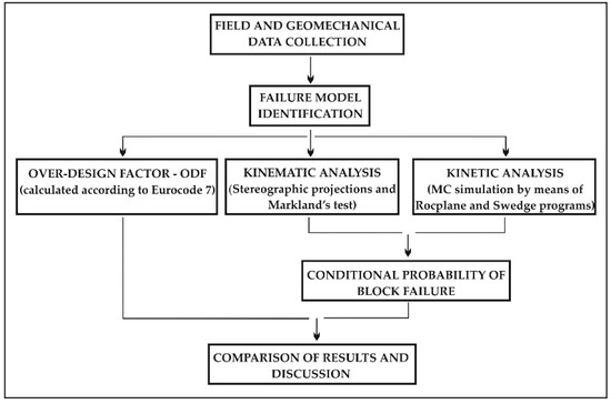
Figure 1.
Flowchart showing the adopted procedure.
3. Geological Setting
The studied slopes are located in a coastal area of the Cilento region (Southern Italy) where dolomitic limestones outcrop (see Figure 2).
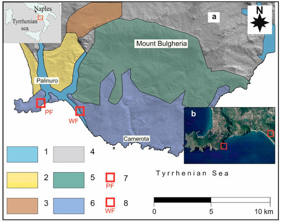
Figure 2.
Schematic lithological map of the Cilento region (a). Key: (1) Alluvial deposits (Quaternary); (2) Conglomerates (Pliocene); (3) Arenaceous-pelitic flysch (Miocene); (4) Marly-clayey flysch (Tertiary); (5) Limestones (Mesozoic); (6) Dolomitic limestones (Trias); (7) slope potentially affected by plane failures of rock blocks; (8) slope potentially affected by wedge failures of rock blocks (modified by [25]). Satellite image by Google Earth (b).
These rocks are made up of a thick pile (up to 2000 m) of Triassic carbonate rocks, belonging to a paleogeographic domain known as Campano-Lucana Platform [25]. In the study area, these rocks consist of well-bedded dolomitic limestones always heavily fractured due to the presence of direct faults striking NW–SE and NE–SW (Apenninic and anti-Apenninic trends) active between the Middle Miocene and Late Pleistocene [26]. Consequently, the continuity of bedding planes is disrupted and several variously oriented joint systems are present. Stratigraphic and geo-structural settings of the rock outcrops at both studied sites, just about 1.5 km away from each other, are very similar.
4. Results
4.1. Geo-mechanical Characterization
The physical characterization of the dolomitic limestones sampled in the two studied sites was obtained according to the ISRM suggested methods [27], and the main properties of the tested material are reported in Table 1. From calcimetric analyses, it was found that calcite is dominant with respect to dolomite, and the rock can be classified as a microcrystalline dolomitic-limestone. Although a weak relationship there is between porosity and dry density, it is possible to observe that the lower the porosity of material the greater is its dry density.

Table 1.
Main physical properties of the dolomitic limestones. Key: γs = material density; γ = unit weight; γd = dry density; n = porosity; w = water content; μ = mean value; σ = standard deviation.
Concerning the shear strength of clean rock joints, reference was done to experimental data obtained by means of the Hoek’s shear box. Before the testing, on the rock specimens containing natural joint surfaces, the Joint Compressive Strength (JCS) and Joint Roughness Coefficient (JRC) were measured by means of the Schmidt hammer rebound and Barton comb [28]. Data coming from 13 tests gave JCS and JRC mean values of about 20 and 6 MPa (“smooth undulating” joints), respectively. Particularly, the low mean value of JCS testifies the presence of a weathered film on the joint surfaces resulting from wetting–drying cycles affecting discontinuities, in the past. With regard to the basic friction angle (φb) obtained by means of tests on artificial surfaces produced by sawing (see Figure 3a), a constant value equal to 30° was always adopted.
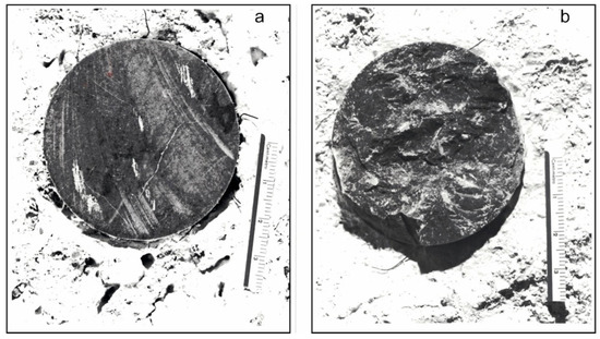
Figure 3.
Photos of joint surfaces after the shear tests. (a) Artificial surface obtained by sawing; (b) natural surface obtained by the splitting method.
According to [7], for reducing the tilting tendency of the upper frame of the shear box, values of the normal stress (σn) in the range 0.25–1.0 MPa were chosen. These values fit well with the normal stresses acting in the rock blocks prone to possible sliding. Experimental data were interpreted by means of the original Barton empirical formula [29] as follows:
Shear tests on natural surfaces prepared by the splitting method (see Figure 3b and Figure 4) gave peak friction angles (φp) in the range 35°–42°, with a standard deviation (σ) of 2.4°. A moderate tendency in φp reduction with increasing normal stress also was detected. It is worth observing that for waviness angles (i) of joint surfaces ranging between 15° and 17.5°, Seidel and Haberfield in [30] obtained φp in the range 39°–42° whereas, for the same asperity angles, Ladanyi and Archambault in [31] calculated φp in the range 37°–39°. Consequently, due to the good agreement between laboratory and literature data, in the following calculations, the experimental peak friction angles were used. Shear strength data refer to joints belonging to both bedding planes and tectonic discontinuities and the few available measurements show low statistical reliability which does not allow to highlight significant differences between joints of different origins. Therefore, in all the adopted stability analyses, peak friction angles fall within the detected range, regardless of whether they were considered failure planes involving stratifications or tectonic joints. Since both studied sites show similar stratigraphic and tectonic features, this shortcoming is not expected to significantly affect the results.
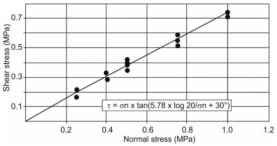
Figure 4.
Peak shear strength envelope concerning data from 13 shear tests.
4.2. Plane Failure
Rock blocks potentially prone to plane failures, selected as the case study example, and the entire slope on which they crop out are shown hereafter (see Figure 5). The slope height is about 20 m with a mean orientation (dip/dip direction) of about 85°/010°.
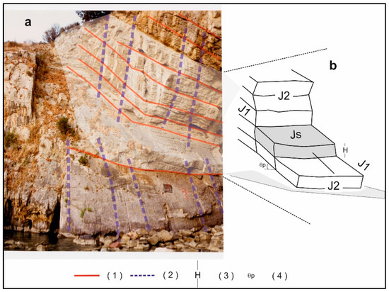
Figure 5.
(a) View of the slope where blocks are potentially prone to plane failures; (b) geometrical model adopted in calculations. Key: (1) discontinuity belonging to the Js joint set; (2) discontinuity belonging to the J1 joint set; (3) block height; (4) dip angle of the Js joint set.
The rock mass is affected by three main joint sets which group the bedding planes (Js joint set) as well as tectonic discontinuities with different orientation (J1 and J2 joint sets). Bedding planes, with a mean orientation of 37°/010°, are in daylight on the slope face whereas J1 joint set (81°/292°) consists of steeply dipping fractures nearly orthogonal to the slope face. These discontinuities represent lateral, planar release surfaces, which provide the least resistance to the potential sliding masses. Joints belonging to the set J2 (85°/200°) show strikes nearly parallel to the slope face and steeply dipping into the face. Since their planes coincide with the slope face, in Figure 5a, these discontinuities are not representable even though they represent potential tension cracks located on the back of the unstable blocks. All joint intersections between the above-mentioned joint sets define elongated tabular blocks with high kinematic degrees of freedom, prone to possible sliding (see Figure 5b and Figure 6).
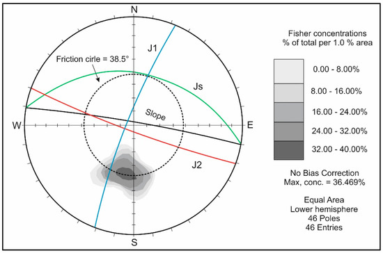
Figure 6.
Kinematic stability analysis for potential plane failures along the Js joint set performed by means of the software program DIPS.
With reference to other physical properties of joints, it can be observed that [1]:
- –
- Joint apertures range from “partly open” to “moderately wide” (0.25–6 mm), but also, apertures up to 10 mm are present. Moreover, some joints show hard calcite veins infilling;
- –
- The roughness, measured by means of the Barton comb [28], results “smooth undulating” for bedding planes (Joint Roughness Coefficient (JRC) values 5–10), whereas it is “smooth nearly planar” (JRC values 6–8) for joints belonging to the other sets;
- –
- The main joint terminations halt against other discontinuities in the exposure (“J/J type” terminations);
- –
- The joint surfaces are “moderately” weathered, with some rock bridges.
On the basis of the described geo-structural model, the kinematic analysis, based on the Markland’s test, was performed by means of the cyclographic projection of the median plane of the joint set Js (46 poles), also representing the geometry of the whole slope and trace of the friction cone of 38.5°, chosen in the range 35°–42° (see Figure 6).
According to the Markland’s test, any discontinuity pole falling inside the friction circle represents a potential sliding plane if it dips within ±20° in the same direction as the slope face. Consequently, the kinematic plane failure probability (Pkm) is 17/46 = 0.369.
The kinetic stability analysis was carried out using the MC method, iterating the simulation 10,000 times. For each MC simulation concerning every potential plane of failure, an SF was calculated. Contrary to what obtained with the deterministic analysis, where single fixed values (generally, mean values) of orientation and strength parameters are used, in MC each parameter is considered as a random variable and the analysis involving different values for each parameter results in different SF. Consequently, SF itself is a random variable, depending on the adopted input variables, and the performed probabilistic analysis considers the uncertainty in parameters and results [9]. In this study, the orientation of joints, unit weight of the rock and friction angle were considered random variables with normal distributions, whereas the slope angle and block height were assumed as deterministic values. For the block height, the adopted value (1.5 m) is based on the mean spacing of the Js joint set. Enabling the option “probability of failure” in Rocplane, the probabilistic analysis was performed. All statistical parameters concerning the adopted model (slope orientation 85°/010° and block height 1.5 m), in the way they were obtained by Rocplane, are shown in Table 2. The main graphical outputs of the probabilistic analysis are reported in Figure 7.

Table 2.
Calculation parameters used for the probabilistic analysis of blocks prone to plane failures. Key: μ = mean value; σ = standard deviation.
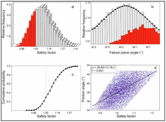
Figure 7.
Results of the probabilistic analysis for planar failure affecting individual blocks. Key: (a) histogram representing the distribution of safety factor, for all valid blocks generated by the Monte Carlo (MC) method. The red bars represent blocks with SF less than 1.00; (b) distribution of failed blocks (red bars) vs. the variation of the failure plane angle; (c) cumulative safety factor distribution giving the probability value that SF will be less than or equal to the value of the variable at that point; (d) relationship between friction angle and SF. Number of simulations = 10,000.
As shown in Figure 7c, the failure probability affecting elongated tabular blocks is 0.293 whereas the value of the correlation coefficient (r) indicates a fair correlation between SF and friction angles (see Figure 7d). This proves that the changing block geometry and dip angle of failure planes have the greatest effect on the failure probability. Unlike “traditional” deterministic analysis, which uses only one set of mean values for the adopted parameters gives SF equal to 1.06 (quite “stable” slope), MC shows that a failure probability characterizes blocks anyway.
If we consider that the kinematic plane failure probability (Pkm) is 0.369 so, the overall failure probability (Pf) is 0.369 × 0.293 = 0.108. That is, this probability is a conditional probability based on the premise that blocks are kinematically unstable.
4.3. Wedge Failure
Several aspects of the slope prone to wedge failures of individual blocks, as well as its geo-structural layout, are shown hereafter (see Figure 8). The entire slope height is about 27 m with a mean orientation of 85°/293°. Although the stratification does not have any influence on the overall stability of blocks, on the contrary, the intersection of joint sets J1 (73°/285°) and J2 (78°/250°) defines wedges with lines of intersection steeply dipping nearly parallel to the slope face (see Figure 8c,d). Due to the adverse geo-structural layout of joints in connection with the slope and presence of morphologies related to already failed wedges, we can say that this slope is prone to a high hazard for future identical landslides.
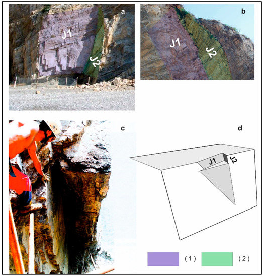
Figure 8.
View of the slope potentially prone to wedge failures. (a,b) wedges already failed along joints belonging to the J1 (violet) and J2 (green) joint sets; (c) morphology caused by an already failed wedge whose line of intersection is nearly vertical; (d) 3D perspective view of the model adopted in calculations. Key: (1) joint surface belonging to the J1 joint set; (2) joint surface belonging to the J2 joint set.
The stereo plot showing great circles of joints belonging to the two above-mentioned joint sets allowed the identification of about 884 intersections defining the potential wedge blocks of which the mean line of the intersection has a trend/plunge of 297°/73°. By means of the Markland’s test, 205 critical intersections of wedge-shaped blocks were identified. These intersections fall in the shaded area between the slope face and trace of friction cone with a value of 38.5° (see Figure 9). Consequently, for these blocks, the kinematic probability (Pkm) is 205/884 = 0.231.
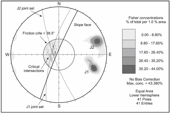
Figure 9.
Kinematic stability analysis, performed by means of the Markland’s test, for potential wedges defined by the intersections between the great circles of joints belonging to the J1 and J2 joint sets.
By means of the Swedge program, the kinetic stability analysis was carried out using the parameters shown in Table 3. In this case, the wedge height (5.0 m) and unit weight of the rock (26.5 kN/m3) were considered as deterministic values. On the contrary, all geometric parameters of wedges and friction angles were considered as random variables with normal distributions. Here again, in the Swedge the option “probability of failure”, for the number of the same simulation (N = 10,000) as for plane failures, was enabled.

Table 3.
Calculation parameters used for the probabilistic analysis of blocks prone to wedge failures. Key: μ = mean value; σ = standard deviation.
The main results of the probabilistic analysis for wedge failures are shown in Figure 10.
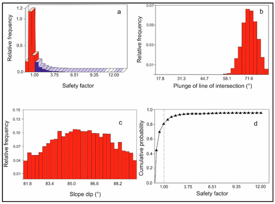
Figure 10.
Results of the probabilistic analysis for wedge failures. Key: (a) histogram showing the distribution of safety factor, for all valid wedges generated by MC of the input data. The red bars represent blocks with SFs less than 1.00; (b) relative frequency distribution of failed wedges vs. the variation of the plunge of the line of intersection dip; (c) relative frequency distribution of failed blocks vs. the variation of the slope angle; (d) cumulative safety factor distribution giving the probability that SF will be less than or equal to the value of the variable at that point. Number of simulations = 10,000.
A failure probability of 0.802 has been calculated (see Figure 10d). In spite of geometrical parameters of the model being assumed randomly, all resulting wedges may slip on both J1 and J2 planes. For the plane J1 (mean dip angle = 73°) the higher relative frequency of failing blocks is in the range of dip angles 70°–77°, whereas for the plane J2 (mean dip angle = 78°) this occurs within the range 72°–81°. For the plunge of the line of intersection, the higher relative frequency of failing wedges is in the range 67–81° (see Figure 10b), whereas for the slope dip similar values are in the range 83°-87° (see Figure 10c).
The overall conditional failure probability (Pf), given by the product of the probability of kinematical instability and the kinetic instability, is 0.231 × 0.802 = 0.185.
5. Discussion
Deterministic ODFs and probabilistic results for both plane and wedge failures are shown in Table 4. According to Eurocode 7, the mean values of each random variable together with the partial factors selected in Tables A.2 and A.3 [17] are used and single ODFs are calculated. On the contrary, the random properties of a random variable in the probabilistic analysis are considered and the final probability of failure, according to the above-mentioned procedure, has been evaluated.

Table 4.
Comparison of results for the deterministic probabilistic analysis of plane and wedge failures.
With reference to the plane failure, the result of calculations performed by means of Eurocode 7 shows that the serviceability limit state requirement is not satisfied, whereas, with the “traditional” safety factor (SF = 1.06), the slope is quite stable. The kinematic analysis, performed by means of the Markland’s test, indicated a failure probability of 36.9%, whereas the kinetic probability is 29.3% because dip angles of Js (failure planes) are lower than the maximum assumed value for the random variable φp. On the premise that blocks are kinematically unstable, the overall conditional probability of plane failure is 10.8%.
Additionally, with regard to the wedge failure, the serviceability limit state is not satisfied (ODF = 0.48) and also the “traditional” safety factor points out an unstable slope (SF = 0.62). Concerning the kinetic analysis, the failure probability is greater than the kinematic instability because the scattered orientations of joints give rise to wedges which may slip with contact on both planes J1 and J2. Furthermore, these wedges slip along lines of intersections with angles higher than the maximum value assumed for the random variable φp. The overall conditional probability is 18.5%. Therefore, the landslide hazard degree of this slope is higher than that previously analyzed.
According to Park et al. [9], the rock slope stability of the two studied slopes was evaluated by means of their kinematic and kinetic conditions. This is because an examination of the kinetic condition is conducted only after the kinematic failure is detected. For both the models, in order to calculate the overall failure probability with MC, simply having SF lower than 1.00 is not enough, because intersections between joints also need to be kinematically possible. Combining the two different probabilities, a final failure probability lower than that obtained by the kinetic approach alone is achieved. This is because the kinetic approach, performed with MC, considers all possible joint intersections irrespective of whether some of them do not delimit blocks that can slide.
The two analyzed sites involve rock masses with a very complex geo-structural layout, hence for conducting computational and repeated calculations in MC (also adopting graphical techniques), a great number of stereographic projections would be necessary. Considering the high number of the adopted simulations (10,000), this approach is not suitable. Consequently, the suggested approach seems more feasible, because the probability of kinetic instability is evaluated only for the potentially kinematic unstable blocks. Final results also show a good fit with the suggested values concerning the levels of acceptance for rock slopes shown in the literature [16].
The used approach, originally proposed in [9], has proven to be very reliable in probabilistic rock slope stability analysis when aiming to incorporate the variability and uncertainty of the rock mass properties into the analytical process. For the adopted failure models, this is also supported by the comparison of the results with those concerning recent research [11,32,33]. Particularly, Aladejare and Akeju in [33] proposed a very similar MC-based probabilistic approach in order to explore the effects of the geometric uncertainties in failure models and variability in geo-mechanical parameters on feasible designs of the rock slope.
The comparison between deterministic SF and ODF values showed non-comparable results. The stability evaluated by means of Eurocode 7 is more conservative than the traditional SF since a precautionary approach is already considered in the use of partial factors applied to different components of the analysis. Furthermore, there is an ambiguous definition in the Eurocode for how the characteristic values should be chosen [19]. At present, as updated data in this European Regulation is lacking, this approach has evident shortcomings, because partial factors must be applied to input parameters which are already affected by uncertainties and variability.
6. Conclusions
This study allowed us to verify the feasibility of deterministic and probabilistic stability analyses based on both kinematic and kinetic approaches for two slopes affected by plane and wedge failures, respectively, and comparing obtained Pf values with the levels of acceptance suggested in the literature. As in Europe, the deterministic limit equilibrium analysis must be performed according to the Eurocode 7, it was also possible to ascertain that the stability evaluated by means of ODF is more conservative than the traditional SF since a precautionary approach is already considered in the use of partial factors which must be applied to the analysis. Furthermore, there is an ambiguous definition in the Eurocode for how the characteristic values should be chosen.
Kinematic analysis was carried out using a common stereographic projection technique (the Markland’s test) while kinetic one was performed by means of the MC simulation implemented in Rocplane and Swedge software codes. MC was used as a numerical process for repeated calculations (10,000 simulations) of SF, varying the slope model geometries and geo-mechanical parameters. The overall failure probability Pf was calculated as a conditional probability given by the product of the kinematic and kinetic probabilities based on the premise that blocks are kinematically unstable.
For the implementation of this approach, a great number of correct geometrical, geo-structural and geo-mechanical data are needed. This is particularly true for shear strength data which refer only to a few experimental measurements obtained by means of the Hoek’s shear box. Particularly, it was not possible to highlight significant differences between joints of different origins. Therefore, the probability of slope failure in this study area must be updated on the basis of more in-depth data. The author will focus on this subject in further study.
Despite the limitations this implies, the results show that the proposed approach is effective in incorporating the variability and uncertainties in rock mass properties and slope geometries, in the analysis of rock slope stability. Furthermore, the results agree well with those of recent research describing, for the same analyzed models, the combined use of computer codes and laboratory tests.
Funding
This research received no external funding.
Acknowledgments
The author is grateful to the anonymous reviewers and to the Editor, whose suggestions have helped to enhance substantially the quality of the presentation. The provision of laboratory facilities at the Department of Civil, Architectural and Environmental Engineering of the University of Naples “Federico II” is gratefully acknowledged.
Conflicts of Interest
The author declares no conflicts of interest.
References
- International Society for Rock Mechanics and Rock Engineering. The Blue Book—The Complete ISRM Suggested Methods for Rock Characterisation, Testing and Monitoring: 1974–2006; Ulusay, R., Hudson, J.A., Eds.; ISRM & Turkish National Group of ISRM: Ankara, Turkey, 2007. [Google Scholar]
- Gibson, W. Probabilistic methods for slope analysis and design. Aust. Geomech. 2011, 46, 1–12. [Google Scholar]
- Chen, S.L.; Cheng, C.P. Influence of failure probability due to parameter and anchor variance of a freeway dip slope slide—A case study in Taiwan. Entropy 2017, 19, 431. [Google Scholar] [CrossRef]
- El-Ramly, H.H.; Morgenstern, N.R.; Cruden, D.M. Probabilistic slope stability analysis for practice. Can. Geotech. J. 2002, 39, 665–683. [Google Scholar] [CrossRef]
- Park, H.; West, T.R. Development of a probabilistic approach for rock wedge failure. Eng. Geol. 2001, 59, 233–251. [Google Scholar] [CrossRef]
- Markland, J.T. A Useful Technique for Estimating the Stability of Rock Slopes When the Rigid Wedge Sliding Type of Failure Is Expected; Imperial College of Science & Technology: London, UK, 1972; p. 20. [Google Scholar]
- Goodman, R.E. Introduction to Rock Mechanics; Wiley: New York, NY, USA, 1989; p. 562. [Google Scholar]
- Hocking, G. A method for distinguishing between single and double plane sliding of tetrahedral wedges. Int. J. Rock Mech. Min. Sci. 1976, 13, 225–226. [Google Scholar] [CrossRef]
- Park, H.; West, T.R.; Woo, I. Probabilistic analysis of rock slope stability and random properties of discontinuity parameters, interstate highway 40, Western North Carolina, USA. Eng. Geol. 2005, 79, 230–250. [Google Scholar] [CrossRef]
- Einstein, H.H. Risk and risk analysis in rock engineering. Tunn. Undergr. Space Technol. 1996, 11, 141–155. [Google Scholar] [CrossRef]
- Obregon, C.; Mitri, H. Probabilistic approach for open pit bench slope stability analysis—A mine case study. Int. J. Min. Sci. Technol. 2019, 29, 629–640. [Google Scholar] [CrossRef]
- Mat Radhi, M.S.; Mohd Pauzi, N.I.; Omar, H. Probabilistic Approach of Rock Slope Stability Analysis Using Monte Carlo Simulation. In Proceedings of the International Conference on Construction and Building Technology, Kuala Lumpur, Malaysia, 16–20 June 2008; pp. 449–469. [Google Scholar]
- Budetta, P.; de Luca, C. Wedge failure hazard assessment by means of a probabilistic approach for an unstable sea-cliff. Nat. Hazards 2015, 76, 1219–1239. [Google Scholar] [CrossRef]
- Zhao, H.; Li, Z.; Kong, C.S. Probabilistic method to determine the overall rock block failure based on failure mode. Eng. Trans. 2016, 64, 105–113. [Google Scholar]
- Mostyn, G.R.; Li, K.S. Probabilistic slope analysis-state of play. In Proceedings of the Conference on Probabilistic Methods in Geotechnical Engineering, Canberra, Australia, 10–12 February 1993; pp. 89–109. [Google Scholar]
- Read, J.; Stacey, P. Guidelines for Open Pit Slope Design; CSIRO Publishing: Collingwood, Australia, 2009; p. 487. [Google Scholar] [CrossRef]
- European Standard EN 1997-1. Eurocode 7: Geotechnical Design—Part. 1: General Rules; European Committee for Standardisation (CEN): Brussels, Belgium, 2004; p. 168. Available online: http://eurocodes.jrc.ec.europa.eu/ (accessed on 3 December 2019).
- Hoek, E.; Bray, J. Rock Slope Engineering, 3rd ed.; Taylor & Francis: London, UK, 1981; p. 357. [Google Scholar]
- Nilsen, B. Rock slope stability analysis according to Eurocode 7, discussion of some dilemmas with particular focus on limit equilibrium analysis. Bull. Eng. Geol. Environ. 2017, 76, 1229–1236. [Google Scholar] [CrossRef]
- Cherubini, C.; Vessia, G. Reliability analyses of rock slope stability. In Proceedings of the 2nd Int Symp on Geothecnical Safety and Risk, Gifu, Japan, 11–12 June 2009; pp. 83–88. [Google Scholar]
- Rocscience Inc. DIPS An Interactive Analysis of Orientation Based Geological Data Software Program (Version 7); Toronto, ON, Canada, 2016. Available online: http://www.rocscience.com (accessed on 12 December 2019).
- Wyllie, D.C.; Mah, C.W. Rock Slope Engineering Civil and Mining, 4th ed.; Taylor & Francis e-Library: London, UK, 2005; p. 431. Available online: https://civilenglineering.files.wordpress.com/2014/10/rock_slope_engineering_civil_and_mining.pdf (accessed on 3 December 2019).
- Rocscience Inc. ROCPLANE (Version 4.001) and SWEDGE (Version 7.001) Software Programs. Toronto, ON, Canada. 2019. Available online: http://www.rocscience.com (accessed on 16 December 2019).
- Grenon, M.; Hadjigeorgiou, J. A design methodology for rock slopes susceptible to wedge failure using fracture system modelling. Eng. Geol. 2008, 96, 78–93. [Google Scholar] [CrossRef]
- Bonardi, G.; Ciarcia, S.; di Nocera, S.; Matano, F.; Sgrosso, I.; Torre, M. Carta delle principali unità cinematiche dell’Appennino meridionale-Nota illustrative. Italian J. Geosci. 2009, 128, 47–60. (In Italian) [Google Scholar]
- Scrocca, D. Southern Apennines: Structural Setting and Tectonic Evolution. J. Virtual Explor. 2010. Available online: http://virtualexplorer.com.au/article/2009/225/southern-apennines-evolution (accessed on 9 January 2020). [CrossRef]
- International Society Rock Mechanics (ISRM). Suggested Methods for Determining Water Content, Porosity, Density, Absorption and Related Properties and Swelling and Slake-Durability Index Properties; Pergamon Press Ltd.: Oxford, UK, 1977; pp. 143–151. [Google Scholar]
- Barton, N.R.; Choubey, V. The shear strength of rock joints in theory and practice. Rock Mech. 1977, 10, 1–54. [Google Scholar] [CrossRef]
- Barton, N.R. The shear strength of rock and rock joints. Int. J. Mech. Min. Sci. Geomech. Abstr. 1976, 13, 1–24. [Google Scholar] [CrossRef]
- Seidel, J.P.; Haberfield, C.M. The application of energy principles to the determination of the sliding resistance of rock joints. Rock Mech. Rock Eng. 1995, 28, 211–226. [Google Scholar] [CrossRef]
- Ladanyi, B.; Archambault, G. Simulation of shear behaviour of a jointed rock mass. In Proceedings of the 11th U.S. Symposium on Rock Mechanics, Berkeley, CA, USA, 16–19 June 1969; pp. 105–125. [Google Scholar]
- Basahel, H.; Mitri, H. Probabilistic assessment of rock slopes stability using the response surface approach-A case study. Int. J. Min. Sci. Technol. 2019, 29, 357–370. [Google Scholar] [CrossRef]
- Aladejare, A.E.; Akeju, V.O. Design and sensitivity analysis of rock slope using Monte Carlo simulation. Geotech. Geol. Eng. 2020, 38, 573–585. [Google Scholar] [CrossRef]
© 2020 by the author. Licensee MDPI, Basel, Switzerland. This article is an open access article distributed under the terms and conditions of the Creative Commons Attribution (CC BY) license (http://creativecommons.org/licenses/by/4.0/).