Abstract
A key point of landslide hazard assessment is the estimation of their runout. Empirical relations linking angle of reach to volume can be used relatively easily, but they are generally associated with large uncertainties as they do not consider the topographic specificity of a given study site. On the contrary, numerical simulations provide more detailed results on the deposits morphology, but their rheological parameters can be difficult to constrain. Simulating all possible values can be time consuming and incompatible with operational requirements of rapid estimations. We propose and compare three operational methods to derive scaling power laws relating the landslide travel distance to the destabilized volume. The first one relies only on empirical relations, the second one on numerical simulations with back-analysis, and the third one combines both approaches. Their efficiency is tested on three case studies: the Samperre cliff collapses in Martinique, Lesser Antilles (0.5 to m), the Frank Slide rock avalanche ( m) and the Samperre cliff collapses in Martinique, Lesser Antilles (0.5 to m) the Fei Tsui debris slide in Hong Kong ( m). Purely numerical estimations yield the smallest uncertainty, but the uncertainty on rheological parameters is difficult to quantify. Combining numerical and empirical approaches allows to reduce the uncertainty of estimation by up to 50%, in comparison to purely empirical estimations. However, it may also induces a bias in the estimation, though observations always lie in the 95% prediction intervals. We also show that empirical estimations fail to model properly the dependence between volume and travel distance, particularly for small landslides (<20,000 m).
1. Introduction
Landslide hazard assessment is the estimation of the probability that an area is impacted by a landslide of given intensity during a given period of time [1,2]. It relies on the evaluation of landslide susceptibility (i.e., the likelihood that a given type of landslide occurs in a given area) and intensity. The definition of intensity depends on the propagation mechanism [1], but generally includes the runout (or travel distance), the velocity and volume of the landslide. These characteristics are commonly estimated from empirical relations (in most case, power laws) depending on the landslide volume, e.g., [3,4,5,6,7,8,9]. However, in order to get more insight on the landslide dynamics, physical model must be used. The most simple one is the rigid sliding block model for which an analytical solution can be derived [10]. Analytical solutions for one-dimensional dam-break problems have also been proposed in [11], and used for instance in [5] to estimate landslide travel distances. Flow routing algorithms implemented in Geographic Information Systems (GIS) softwares combine probabilistic methods and semi-empirical energy dissipation laws to reproduce multiple channelling and mass spreading [12,13]. Nevertheless, physically-based numerical modeling is needed to reproduce the complex mechanisms governing landslide propagation. 3D modeling allows to describe precisely the interactions between fluid and/or solid particles [14,15,16] but is often computationally costly and relies on many user-defined parameters, which are in practice difficult to estimate.
In comparison, thin-layer models (also commonly called shallow-water models) integrate the momentum equations over the flow thickness of fast-propagating landslides, whose thickness is negligible in comparison with their extent. Thus, the state variables are reduced to the flow thickness and thickness-averaged velocity and simulations can be run faster than full 3D models. In their most simple form, the shallow-water equations describe the evolution of a homogeneous flow and use a solid Coulomb friction law to model the interaction between the topography and the flow, through a friction coefficient . The stress applied at the base of the flow, that decelerates the flow, can also be modeled with the Voellmy rheology that includes a turbulence term [17,18], or the Bingham rheology for yield-stress fluids [19]. More complex shallow-water models include, for instance, erosion and deposition along flow path [20,21] and two-phase flows with dilatancy effects [22,23,24,25].
In this work, we aim at developing and comparing methodologies to estimate the travel distance of rapid gravity-driven flows [5,18,26] depending on their volume. The resulting relations must be simple enough to be used operationally by practitioners. They can be established simply by using mobility indicators such as the Heim’s ratio or the effective friction coefficient [5]:
H is the drop height, the horizontal travel distance along flow path, the average slope along flow path, the initial mass maximum height and the travel distance along topography from the collapse scar toe (Figure 1). is less straight-forward to use than as it takes into account the geometry of the initial mass, which is not always easy to estimate.
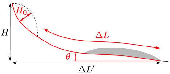
Figure 1.
Parametrization of landslide mobility, with notations as in [5]. Dashed line: initial mass. Grey shaded are: final landslide deposits. H is the drop height, the horizontal travel distance. is the mass initial thickness, the travel distance along topography from the landslide scar toe, and is the average slope angle along the flow path. The notations in red are used for , and in black for .
The empirical estimations relating the landslide volume to or rely on large datasets that are not, in general, site specific. Thus, the particular topographic setting of a given study site is not taken into account. This often results in large uncertainties that are however relatively simple to evaluate from the residuals between the fitted model and the observations.
In comparison, numerical modeling and in particular shallow-water models are commonly-used to carry out site-specific hazard analysis, e.g., [27,28,29]. However, many simulations (up to 1000 or even 10,000) are needed to perform a rigorous probabilistic hazard analysis, e.g., [30]. Besides, estimating parameters can be difficult, or at least time consuming and costly, which is often incompatible with operational constraints where hazard assessment must be carried out quickly. Rheological parameters can be estimated by back-analysis when previous events are documented, but the extent to which results can be used for forward prediction is hard to constrain [28]. Rheological parameters can also be empirically deduced from mobility indicators. In particular, the effective friction coefficient , whose definition differs from the Heim’s ratio as it takes into account the initial mass geometry, proved to be a relatively good estimation of the friction coefficient to be used in simulations needed to model observed deposits [5].
In this context, the extent to which numerical modeling can improve the estimation of landslide runout in comparison with empirical approaches, has, to our knowledge, never been quantified. To answer this question, we will derive site-specific power laws relating the horizontal travel distance to the unstable volume V, using a purely empirical approach, a numerical approach and combining empirical data with numerical modeling. Empirical data is drawn from two landslides databases ([3,5,31]). Numerical modeling is carried out with the SHALTOP shallow-water numerical model [32,33,34]. We will use a simple Coulomb friction law that proved, with SHALTOP, to reproduce successfully real landslides deposits [5,29,35,36,37,38]. Besides, this rheology involves a single parameter, which simplifies uncertainty analysis. We compare the prediction and associated uncertainties for three documented case studies: rock/sand avalanches from the Samperre cliff in Martinique, Lesser Antilles, the Frank Slide rock avalanche in Canada and the Fei Tsui Road debris slide in Hong-Kong.
2. Materials and Methods
2.1. Data
We present here the case studies on which methods of travel distance estimations will be compared. Empirical methods are based on empirical estimations of mobility deduced from databases of landslides landslide databases. In comparison, numerical methods rely on databases of simulations that we construct for each case study site-specific simulation databases.
2.1.1. Case Studies
In this work we focus on three landslides case studies, spanning a large range of volumes and runouts. Their characteristics are summurized summarized in Table 1.
Destabilizations from the Samperre cliff, in Martinique, Lesser Antilles, involve volumes between 1 and m [39,40] that propagate on a complex topography (Figure 2a,b). As they detach from the cliff, old pyroclastic materials erupted from the nearby Montagne Pelée volcano desegregate rapidly and the landslide propagates as a granular avalanche. Massive destabilizations occur roughly every 10 years, as in 2009 and 2018 [39,40] and travel about 2 km in the Samperre torrent that has its source at the cliff toe (Figure 2c). The stream flows in a narrow (no more than 40 m wide) and steep-walled (up to 70 m high banks) ravine that confines laterally the avalanche. The volume involved in the August 2009 collapse is estimated at m in [39]. In 2018, the main destabilization phase occurred in early January, and involved at most m [41], as deduced from 1-m Digital Elevation Models (DEMs) comparisons between July 2017 (LiDAR) and mid-January 2018 (photogrammetric reconstruction). However, considering the cliff retreat between these two dates, we estimate a smaller m volume (see Appendix A).
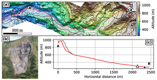
Figure 2.
Samperre cliff destabilizations. (a) August 2018 topography, 1 m DEM. Black dashed outline: extent of destabilized area (difference between 2010 and 2018 DEMs). Bold contour interval is 100 m. Red line: cross-section along which travel distances are measured. Black triangle: observed travel distance in 2009. White triangle: observed travel distance in 2018. (b) Picture of the Samperre cliff (black dashed outline in (a)) taken in February 2018 (OVSM). (c) Cross-section along red line in (a). Red line: Post-collapse topography with deposits removed. Black dashed line: Topography in July 2010. Black and white triangles are reported from (a).
In comparison, the Frank Slide rock avalanche features a larger volume: m. It is more easily constrained than the Samperre destabilizations, because it consisted in a single event that occurred in 1902 on the east face of Turtle Moutain in western Alberta, Canada (Figure 3a,b). It involved mainly Paleozoic limestones that slid along the dipping bed of Turtle Mountain anticline [42]. The rock avalanche covered approximately 2.6 km and traveled about 3 km (from the rear scar) without confinement. The scar displays 30 to 60 slopes, but the topography flattens quickly at the mountain toe. The rock avalanche then ran slightly uphill on the other side of the valley with slopes no higher than 3 (Figure 3c).
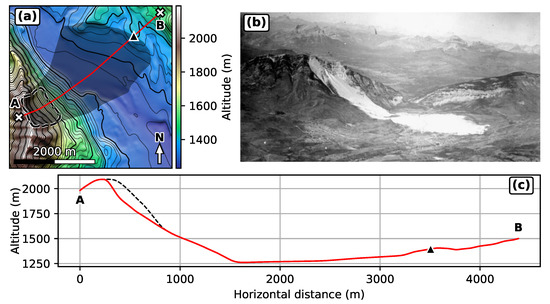
Figure 3.
Frank Slide rock avalanche. (a) Post collapse topography with deposits removed, 20 m DEM. Black dashed outline: landslide scar. Dark area: observed landslide extent. Bold contour interval is 100 m. Red line: cross-section along which travel distances are measured. Dark triangle: Observed travel distance. (b) Picture of the Frank Slide, taken in 1922 (Canada. Dept. of National Defence/Library and Archives Canada/PA-052095). (c) Cross-section along red line in (a). Red line: Post-collapse topography with deposits removed. Black dashed line: Reconstructed pre-collapse topography. Black triangle: observed deposit extent.
The 1995 Fei Tsui Road debris slide case-study differs significantly from the previous ones (Figure 4). It occurred in Hong-Kong after intense rainfalls: more than 1300 mm in the preceding month and 230 mm in the preceding 12 h [43]. It involved 14,000 m of debris, which is unusually high for landslides in Hong-Kong [43,44]. The debris slide originated form a 30 m high cut slope in moderately to highly weathered volcanic materials, with the base of the scar following a kaolinite-rich altered tuff layer. It is assumed that the development of a 1 to 4 m high perched aquifer above the kaolinite-rich layer favored the initiation of the landslide as a translational slide. As a result of low cohesion values [43], the material then desegregated rapidly. The debris slide traveled about 65 m (30 m from the scar toe) with limited spreading, with some of the deposits piled up against the corner of a building.
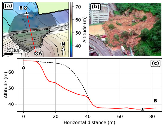
Figure 4.
Fei Tsui Road debris slide. (a) Post collapse topography with deposits removed, 1 m DEM. Black dashed outline: landslide scar. Dark area: observed landslide extent. Bold contour interval is 10 m. Red line: cross-section along which travel distances are measured. Dark triangle: Observed travel distance. (b) Picture of Fei Tsui Road debris slide (GEO, Hong-Kong). (c) Cross-section along red line in (a). Red line: Post-collapse topography. Black dashed line: Reconstructed pre-collapse topography with deposits removed. Black triangle: observed deposit extent.

Table 1.
Description of the case studies considered in this work. We give the characteristics of the documented landslides and of the simulation databases. gives the effective friction coefficient estimated from the landslide volume, using the power law deduced for DB1 (see Figure 5b). For the Samperre case study, we give the estimated volumes and travel distances for the 2009 and 2018 collapses (date in brackets).
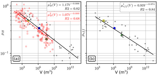
Figure 5.
Empirical landslide databases. (a) VS landslide volume V. Grey circles: DB1. Red marker: DB2. squares: rockfalls and rockfalls avalanches from [3]. Triangles: debris flow, debris slides and debris avalanches from [3]. Crosses: Rock avalanches from [31]. Black line: power law regression result for DB1 (equation given in black). Red dashed line: power law regression result for DB2 (equation given in red). (b) VS landslide volume V, for DB1. Black line: power law regression result for DB1 (equation given in black). Yellow circle: observations for Fei Tsui Road debris slide. Blue circle: observations for the most import destabilization of the Samperre cliff in 2018. Green circle: observations for the Franks Slide.
Table 1.
Description of the case studies considered in this work. We give the characteristics of the documented landslides and of the simulation databases. gives the effective friction coefficient estimated from the landslide volume, using the power law deduced for DB1 (see Figure 5b). For the Samperre case study, we give the estimated volumes and travel distances for the 2009 and 2018 collapses (date in brackets).
| Samperre Cliff Collapses [39,40,45] | Frank Slide Rock Avalanche [42] | Fei Tsui Road Debris Slide [43,44] | ||
|---|---|---|---|---|
| DOCUMENTED EVENT | Volume (V) | m (2009) m (2018) | m | m |
| (2009) (2018) | ||||
| Observed horizontal travel distances () | 2100 m (2009) 2000 m (2018) | 3200 m | 65 m | |
| Best-fit friction coefficient | ||||
| SIMULATION DATABASE | Range of volumes V | m to m | m to m | m to m |
| Range of friction coefficients | to | to | to | |
| Simulation grid size | ||||
| Simulation grid resoultion | 5 m | 20 m | 1 m | |
| Number of simulations | 165 | 137 | 91 | |
| Maximum duration for one simulation | 12 h | 30 min | 10 min | |
2.1.2. Landslide Databases
We use two databases to estimate empirically travel distances. The first one (DB1) is drawn from [5]. It includes 43 dense and rapid landslides from Earth, Mars, Iapetus (Saturn’s satellite) and Io (Jupiter’s satellite). Both the Frank Slide and the Fei Tsui Road debris slide are included in DB1. The second database (DB2) combines 44 rockfalls, rockfalls avalanches, debris flows, debris slides and debris avalanches drawn from [3], as well as 49 rock avalanches drawn from [31].
From these databases we fit two power laws relating to the landslide volume V: for DB1 and for DB2. Only DB1 could be used to derive a relation between and V, , because the measures field observations required to compute are not available in DB2. The regression results are given in Figure 5. More details on the regressions quality are available in Table A1. Note that our power law differs from the power law derived in [5] because we fit a power law without constraining , while in [5] is imposed.
2.1.3. Simulation Databases
For each case study, we construct a simulation database with the SHALTOP shallow-water numerical code [32,33,34]. This is done by considering multiple initial unstable geometries and friction coefficients . For each case study, we model destabilized volumes ranging from 1/3 one third to about twice the volumes involved in documented events. The range of tested encompasses realistic coefficients estimated from expert knowledge, in regard of the volumes considered. In particular, the value (with V the volume of the real landslide, see Table 1) is also tested: it has been shown to be a good estimate of the friction coefficient needed to reproduce the landslide dynamics and deposits [5,36,37]. The lowest value is also constrained by practical considerations: for small , the landslide does not stop within the simulation grid and no travel distance can be measured. The main characteristics of the simulations are given in Table 1.
For the Samperre cliff case study, several topographic surveys were carried out over the years: they allow to quantify the evolution of the cliff after collapses episodes, but no data are available to constrain precisely individual events. Thus, we have inferred a total of 10 initial volumes/geometries spanning volumes from m to m: two of them are used to reproduce the August 2009 ( m) and January 2018 m major events. More details about the definition of collapse scenarios are given in Appendix A. Friction coefficients are chosen between and every 1°, and every up to . This results in a total of 165 simulations. The best-fit friction coefficients used in simulation to reproduce the travel distance of the 2010 and 2018 events are and , respectively. Given the relative poor constraints we have on the 2010 event, in particular in term of initial geometry (see Appendix A), we suggest the second fit is more accurate. Thus, we will use in the following intermediate value that is closer to the 2018 event back-analysis.
For the Frank Slide and Fei Tsui Road case studies, simulations are run on 20 and 1 meter DEMs, respectively. They were provided (along with the initial mass of the past landslides) for the First JTC1 Benchmarking Exercise [46]. In comparison to the Samperre case study, we use a more simple way of simulating various volumes. Indeed, we simply scale uniformly the heights of the real destabilized mass to explore larger and smaller volumes. For the Frank Slide, in addition to the real m landslide, we test 67 other volumes spanning from 10 to m, every m. Friction coefficients are taken between and , every 1°. This amounts to 137 simulations. The best-fit friction coefficient used in simulation to reproduce observed deposits resulting from the historical m landslide is , as in [35].
For the Fei Tsui Road debris slide, we test volumes spanning regularly between 5000 and 30,000 m, every 5000 m, and the real 14,000 m volume. Friction coefficients are chosen between and every 1°, resulting in 91 simulations. The best-fit friction coefficient used in simulation to reproduce the 2018 m debris slide is , as in [35].
Simulations are run on the S-CAPAD DELL cluster of the IPGP, on CPU Power Edge C6220, PowerEdge R720xd or PowerEdge R730xd nodes. 128 nodes were thus available, each one with 16 cores. In turn, simulations could be run simultaneously (one simulation per core). Each simulation lasts between 10 min (in the Fei Tsui Road case study) and 12 h (in the Samperre case study). Note that the total number of simulations remains small in comparison with what would be needed for a thorough analysis of uncertainty (i.e., at least 1000 simulations [30]). Nevertheless, it is compatible with time constraints met by practitioners who must carry out quick hazard assessment.
For each case study, we use the simulations results to compute site-specific power laws relating the horizontal travel distance to the initial volume V and the friction coefficient : . For each simulated deposits, we can also compute the resulting from (2). For clarity, values derived from simulations results will be noted , while refers to values deduced from real landslides. Their definition is however the same. In turn, we can compute another power law relating to V and : . The data used to derive and are given in Supplementary Materials.
2.2. Estimation of Horizontal Travel Distances
We use three different methods to estimate the horizontal travel distance directly from the landslide volume V. They are summarized in Figure 6. We use empirical data from DB1 or DB2, site-specific numerical simulations or a combination of the two. For the sake of clarity and simplicity, we do not explicit the functions that will be mentioned hereafter. It can be any kind of statistical model fitted to the landslide travel distances databases, or to the numerical simulations results, provided the associated uncertainties can be estimated. In this work, we use power law relations that are fitted by transforming the variables on a logarithm scale and by fitting a linear regression model using Ordinary Least Square (OLS) regressions (see more details in Appendix B). Thus, the final relation relating to V has the form:
where the coefficients and depend on the studied site and on the chosen methodology.
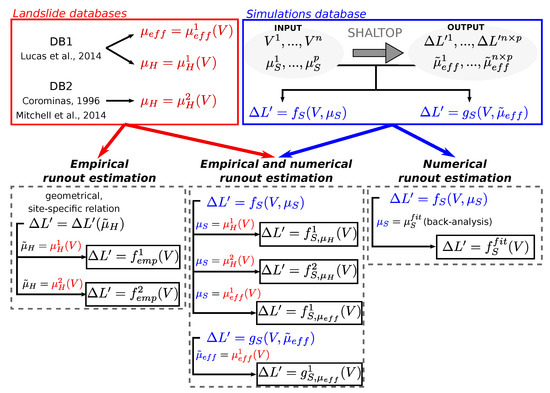
Figure 6.
Methodologies to derive volume dependent relations for travel distance estimation. The superscripts and refer to the empirical database that is used for a given relation (DB1 and DB2, respectively). In this study, all functionals are power laws.
2.2.1. Empirical Runout Estimation
For a given study site, we choose a profile along which travel distances will be measured, in the main direction of propagation of observed landslides (red lines in Figure 2a,c, Figure 3a,c and Figure 4a,c). Provided an origin is chosen, a ratio can be computed for each point along the profile. Thus, we do not need to run simulations. However, in practice, it is convenient to compute for the points that are reached by landslides in our simulations. As the modeled stopping points span a large portion of the profile, it is equivalent to choosing manually points along profiles and the resulting relation does not depend on the simulations. Besides, for the Samperre cliff simulations in particular, this allows to take directly into account the variability of the profile, as we consider different collapse geometries.
If the topography is convex, which is the case in our three case studies, it is possible to invert the previous relation to derive from : . Note that is computed geometrically. We relate it to realistic landslide mobilities by choosing , where is the Heim’s ratio measured on real landslides. Using the volume dependent relations deduced from the empirical databases DB1 and DB2, and , we get:
which we will write more simply
In comparison, it is more difficult to use for direct empirical estimation as its definition includes a more complex topography description (the mean slope along flow path) and the initial geometry and volume (through the initial height ). Thus, it is not straight-forward to invert (2) to get a relation . However, this can be done through simulations, as will be explained in Section 2.2.3.
Not that we could also have used empirical power laws derived directly from landslide databases, and apply them directly on each case study. We choose not to, because such a method does not yield a site-specific power law. In comparison, can be deemed to be, in a first approximation, a good mobility indicator, that can then be used on a chosen site. We will however compare in Section 4.3 relations found in the literature, to the site-specific laws derived in this study.
2.2.2. Numerical Runout Estimation
The travel distance can also be estimated without using empirical mobility indicators. For each study site, we derived from the simulation results a statistical relation . As we want our final relation to depend only on V, we must choose a value for . It can be done by modeling a past landslide for which both the initial volume and the travel distances are known. By choosing for the best-fit friction coefficient , and assuming that it does not depend on the landslide volume, we then get a volume only dependent relation:
However, if no past event is available for back-analysis, we can use empirical observations.
2.2.3. Numerical/Empirical Runout Estimation
In the relation deduced from a simulation database, we can choose as a function of the volume. As a matter of fact, it has been shown that lower friction coefficients are needed to model larger landslides. This can be done by back-analysis of multiple events with various volumes on a same site, but we do not have enough data for that. The other possibility is to consider that the empirical mobility indicators and are good estimates for and setting, respectively , or . Combining these relation with , we derive the volume dependent relations:
Another possibility is not to consider , and use only the simulations results. As a matter of fact, we can compute for each simulated landslide the mobility indicators and . The indicates that they are given by simulation results, when and are computed on real landslides. Their respective geometrical definitions are however the same.
From the simulation database, we can thus estimate a relation , which is the same as for empirical runout estimation (see Section 2.2.1). To be consistent with the definition (2) of that includes both the initial mass geometry and the travel distance, we derive from the simulations results a relation . This is done with the tuples for which lies within the 95% prediction interval of the empirical relation . Other tuples are deemed to be unrealistic. Finally, we use in to derive the relation:
2.3. Estimation of Uncertainty
To derive the uncertainty associated with the estimation of travel distance, we use the dispersion between observed values and values predicted by power laws, and the uncertainty on the power law coefficients. Classical results of linear regression can be used to derive prediction intervals for a given power law, taking both these aspects into account (see Appendix B). However, it is not straight-forward to extend these results for nested power laws, when the result of one is the input of another. Indeed, the final expression of the runout involves the sum and product of random variables that are not independent. Thus, it is not easy to derive formally the final probability density function. Instead, we derive numerically prediction intervals by computing 4000 estimations with coefficients and/or residues of each power law drawn randomly (following probabilistic laws whose parameters are given by the regression). We then derive the 95% prediction interval from the 2.5th and 97.5th percentiles. More details are given in Appendix B.
The normalized standard deviation of the estimation , for a given volume V, is defined as:
where is the direct estimation from the best-fit power law, and are n random estimates. We define the total standard deviation over a range of different volumes as
We choose volumes sampled regularly in logarithmic scale between the minimum and maximum simulated volumes. When we use back analysis for travel distance estimation in , we also take into account for the uncertainty on the best fit friction coefficient . This is done by drawing random values of () with a normal distribution of mean and standard deviation 1°. This value is chosen because it matches the interval between two successive tested values of in simulations, in the neighbourhood of the best-fit friction angle.
3. Results
In this section, we will first present the results of the different power laws that were computed in this study, from empirical data or from simulations results. Then, we will compare, for each case study, the different final estimations giving directly the travel distance as a function of the unstable volume V.
3.1. Quality of Power Law Regressions
In this work, we have used simple power laws to derive statistical models both from empirical databases and simulations results. Their quality can be at first hand assesed from the adjusted R2, but other indicators are needed to assess the reliability of uncertainty estimation. The details of the statistical analyses, with the coefficients and quality indicators, are given in Table A1. The behaviour of residuals depending on predicted values is given in Appendix A (Figure A1 and Figure A2).
The site-specific power laws are associated with very good : 0.91 for for the Samperre case study, and more than 0.97 for other power laws. In comparison, empirical power laws feature values between 0.68 (for DB2) and 0.84 (for DB1). and have a Variance Inflation Factor (VIF) below 1.08, which is a good indication that the explanatory variables are not linearly correlated and that the OLS regression is robust (in the sense that the inversion problem is well-constrained). The linearity hypothesis (that is, the validity of using a linear model to represent the link between the logarithm of the runout with the predictor variables) is also relatively well verified, with residues relatively well centered around 0 (Figure A1 and Figure A2). However, we do see for the Frank Slide case study slightly concave and convex shapes for the residuals curve (Figure A2d–f). In turn, the hypothesis of homoscedasticity of residuals (that is, that the deviation from the regression result is similar for all predictions) is not verified in the Frank Slide case study (p-value of the Breush-Pagan test below 0.04). Finally, while the hypothesis that the distribution of residuals folowws follows a normal law is well verified for all empirical power laws , and , it can be questioned for the site-specific power laws, in particular for and (p-values of the Jarque-Bera test below 0.15).
3.2. Estimation of Travel Horizontal Travel Distances
In Table 2 we summarize the different power laws that were derived to estimate travel distances with different methodologies. In the following we will compare the estimation results for each case study.

Table 2.
Estimations of travel distance depending on destabilized volume V, following a power law . We give the value of the exponent along with the standard deviation of its estimation , and the normalized standard deviation of the prediction see (13) and (14). is the averaged predicted travel distance for volumes between the minimum and maximum volumes used in the simulation databases, in each case study.
3.2.1. Samperre Cliff Case Study
Estimations of travel distances for the Samperre cliff case study are given in Figure 7 and Figure 8. The empirical estimation (that uses directly and DB1) is in good agreement with observations (Figure 7a), but (derived from DB2) slightly over-estimates them (Figure 7c). When we use simulations results with approximated from or (, , in Figure 7b,d,f, respectively), the observed travel distance is systematically under-estimated by at most 40%. Finally the empirical/numerical estimation is in almost perfect agreement with the back-analysis estimation (Figure 7e) and thus with the observations. The exponent is 0.14 for the empirical estimations, and varies between 0.24 and 0.33 for the empirical/numercial and numerical estimations (Table 2).
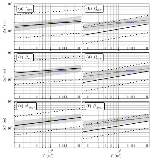
Figure 7.
Travel distance estimated from volume for the Samperre case study. Green and blue rectangles: estimations of volumes and travel distances for the 2009 and 2018 collapses, respectively. Grey line: Numerical estimation from back-analysis (), with . The grey area is the upper and lower limits of the 95% prediction intervals derived for . (a) Estimation with . (b) Estimation with . (c) Estimation with . (d) Estimation with . (e) Estimation with . (f) Estimation with . Black lines are direct estimates, dashed lines give the 95% prediction interval.
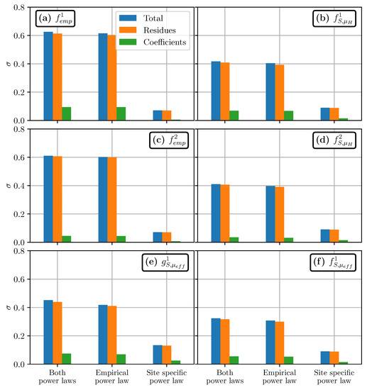
Figure 8.
Uncertainty in travel distance estimation for the Samperre cliff case study, measured by the normalized standard deviation (see main body of the text). is computed by drawing randomly the power laws coefficients (green bars), the residuals (orange bars), or both (blue bars). As each estimation is the combination of two power laws, we consider uncertainties on the first power law derived from empirical databases (middle bars), on the second power law that is derived for the topography and simulation (right bars), or on both (left bars). (a) Estimation with . (b) Estimation with . (c) Estimation with . (d) Estimation with . (e) Estimation with . (f) Estimation with .
Observations lie within the 95% prediction intervals of all estimations (black dashed lines in Figure 7). These intervals delimit the values predicted by the statistical models in 95% of the cases, given the estimated uncertainties (See Appendix B). These intervals are always very large, which can be correlated to high values of the normalized standard deviations in travel distance estimations, (see Table 2). Indeed, we have for empirical estimations, which means that the standard deviation of estimations amounts to 60% of the direct prediction of the power law, when uncertainties are not taken into account. Using Shaltop reduces to 0.4 in empirical/numerical estimations with , and even 0.3 when we choose . When the best-fit friction coefficient is used, drops down to 0.13 (see Table 2). In turn, the 95% prediction interval for is 2 to 3 times smaller than for other power laws.
As described in Section 2.2.3, the final empirical and empirical/numerical estimations of runout uses a first empirical power law, whose result is used in a second site-specific power law. By adding uncertainty in the first or in the second power law, or in both (see Appendix B), we see that most of the uncertainty comes from the empirical relation giving or as a function of volume. This is illustrated graphically in Figure 8, where we see that the total uncertainty is almost the same when we consider uncertainty on both power laws (“Both power laws” blue bars) or on the empirical relation only (“Empirical power law” blue bars): the difference is less than 2%. Besides, most of the uncertainty can be recovered by considering only the deviation between the best-fit power laws, and the data used to derive them. In comparison, the uncertainty on the power law coefficients increases by at most (compare orange and green bars in Figure 8). This can be expected, as we compute for volumes within the range of simulated volumes. If we considered larger or smaller volumes, the uncertainty on coefficients would have more significant effects.
3.2.2. Frank Slide Case Study
The results for the Frank Slide case study are presented in Figure 9. The main conclusions are similar to the Samperre case study. The direct empirical estimations predict correctly the observed travel distance (Figure 9a,c). Using and as input values for in simulations, the observed travel distance are under-estimated by at most a 15% (Figure 9b,d,f, compare blue rectangle and black line).
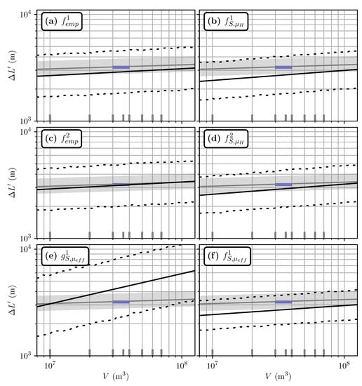
Figure 9.
Travel distance estimated from volume for the Frank Slide case study. Blue rectangle: estimations of volumes and travel distances for 1903 slide the documented event. (a–f), and symbols are the same as for Figure 7.
However, on the contrary to the Samperre case study, the estimation is significantly different from the other estimations. It predicts a travel distance that is about twice the observed travel distance (Figure 9e). The power law exponent is also significantly different: we get only for and , for empirical/numerical estimations, and for the back-analysis estimation. Finally, is associated with larger uncertainties, with . It is even more than the uncertainty for empirical estimations, . As for the Samperre case study, the latter is improved by empirical/numerical estimations, though less significantly ( for and , and for ). Once again, the back-analysis estimation yields the most precise estimation, with .
The analysis of uncertainty propagation (see Figure A3) yields similar conclusions as in the Samperre case study.
3.2.3. Fei Tsui Road Case Study
The results for the Fei Tsui case study are presented in Figure 10. As previously, the direct empirical estimations are coherent with observations (Figure 10a,c). The estimation , that uses the database DB1, only slightly under-estimates the estimation by about 10%. When and are used to estimate in numerical simulations, the observations are all well reproduced (Figure 10b,d,f). To the contrary, the estimation with over-estimates the real travel distance by 45%.
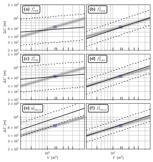
Figure 10.
Travel distance estimated from volume for the Fei Tsui Road case study. Blue rectangle: estimations of volumes and travel distances for 1903 slide the documented event. (a–f), and symbols are the same as for Figure 7.
A major difference between the empirical estimations and other estimations is the value of the power law exponent . For and we compute , but we get or for empirical/numercial estimations. A similar value () is derived for the back-analysis estimation .
Finally, as for the Samperre cliff case study, numerical simulations allow to reduce significantly the estimation normalized standard deviation . When is more about 0.35 for empirical estimations, it is reduced to less than 0.20 with empirical/numerical estimations (down to 0.16 with ). yields the smallest standard deviation, with .
The analysis of uncertainty propagation (see Figure A4) yields similar conclusions as in the Samperre and Frank Slide case studies.
4. Discussion
4.1. Uncertainty of Travel Distances Estimation
4.1.1. Uncertainty Reduction with Numerical Models
A major result of this work is that combining empirical estimations with numerical simulations reduces the standardized standard deviation of estimations. The smallest uncertainty is derived by using back-analysis and a constant friction coefficient, but it is difficult to quantify the uncertainty on the best-fit friction oefficient . As shown in [28], the extent to which it can be used for other landslides is not clear, even considering similar volumes and propagation paths.
This reduction is all the more important as the volumes considered are small. By setting or in , is reduced by 12.5% for the Frank Slide and by 43% for the Fei Tsui Road case study. A similar trend is observed with (reductions by 29% and 54%, respectively). This can be directly correlated to the exponents of in , whose absolute values are systematically higher than the exponents of in (see Table A1). In turn, uncertainty on or results in less deviation in the final empirical/numerical estimations, in comparison with the purely empirical estimation (see Appendix C).
We may argue that as the site-specific power laws do not always verify the hypotheses of OLS regressions, the associated uncertainty estimation (and thus the observed reduction of uncertainty afore-mentionned) is not relevant. However, the estimation of the coefficients of the power laws does not depend on these hypotheses, such that the argument presented in the previous paragraph still stands true. Besides, the residuals of the site-specific power laws are at most between −0.1 and 0.1 (in logarithmic scale), while they span range from −0.3 to 0.3 for the empirical power laws (compare Figure A1 and Figure A2). In turn, even if real uncertainty of site specific laws is higher than what we estimate, it will still be less than the uncertainty associated with empirical, non site-specific power laws. Thus, improving the quality of empirical/numerical travel distance estimations should be done primarily by improving the quality of the empirical power laws.
4.1.2. Quality of Empirical Power Laws Uncertainty Related to Dispersion in Empirical Power Laws
Empirical laws can be improved by considering a database of landslides sharing similar characteristics with the case study. For instance, if we construct DB2 by taking only the debris flows, debris slides and debris avalanches from [3], we derive a new relations with that can be used for the Fei Tsui Road case study (see Figure A5 and Figure A6). As a result, the standard deviation of the travel distance estimation is about 0.25. In comparison, we had for (that is, when we included rockfalls and rock avalanches in DB2). However, removing rockfalls and rock avalanches from DB2 also leads to a 15% over-estimation of the observed travel distance (though it remains in the 95% prediction interval).
Although regrouping landslides by type may increase the quality of the fit, associated hardly exceeds 0.9 (e.g., no more than 0.85 in [5], less than 0.5 in [8], less than 0.2 in [31], and less than 0.8 in [4]). In [3], combining both landslide types and geometrical characteristics of the propagation (i.e., whether the landslide is laterally or frontally obstructed) allows to derive power laws with values between 0.65 and 0.92. Further improvements of the quality of empirical power laws may demand to express more finely the characteristics of the topography upon which the landslide propagates.
4.1.3. Topography Description in Empirical Power Laws Uncertainty Related to Topography Description
To estimate more finely the travel distance in empirical relations, it may be worth using statistical model that do not depend only on the volume. For instance in [31], a relation
is derived from a database of rock avalanches, with . Here, C is an indicator variable with if lateral confinement is observed, and otherwise. In comparison, with the same data, they derive a power law with only. In our work, combining their data with the data of [3] allows to increase the to 0.68 because the resulting database DB2 spans a wider range of volumes.
By estimating the probabilistic distribution of the residues in (15), it is then possible to estimate, for a given topography and volume, the probability that the landslide goes further than a chosen point M on the topography. This is done by considering the difference between the travel distance associated with the point M, and the travel distance predicted by the power law:
Then the probability that the travel distance exceeds , given a volume V, a drop height and a confinement indicator C is:
which can be computed if the distribution of is known. This methodology could be applied in our case: in particular, it allows to skip the derivation of the site-specific relation . However, it should be adapted to consider the uncertainty on the power law coefficients, which was not done in [31]. Besides, using the landslide drop height H as an explanatory variable may favor multi-linearity, as H is correlated to V. For instance in [4], a power law with was derived for volcanic landslides.
A fine description of topography, as well as of the initial unstable mass, is also needed to estimate empirically the friction coefficient of a given landslide. In our empirical/numerical methodologies of travel distance estimations, we used and . The relevance of this choice is discussed in the next section.
4.2. Are and Good Estimates of ?
Comparison with empirical data in [5] shows a good correlation between and over a wide range of volumes. This is not in exact agreement with our results, because we needed , as well as and , to reproduce the Samperre cliff collapse and the Frank Slide, respectively. In simulations, when comparing to and (Figure 11), we find almost systematically that and over-estimate by up to 30%. This is in agreement with results of [29]. The only exception is the Fei Tsui Road case study where we have for m (Figure 11e).
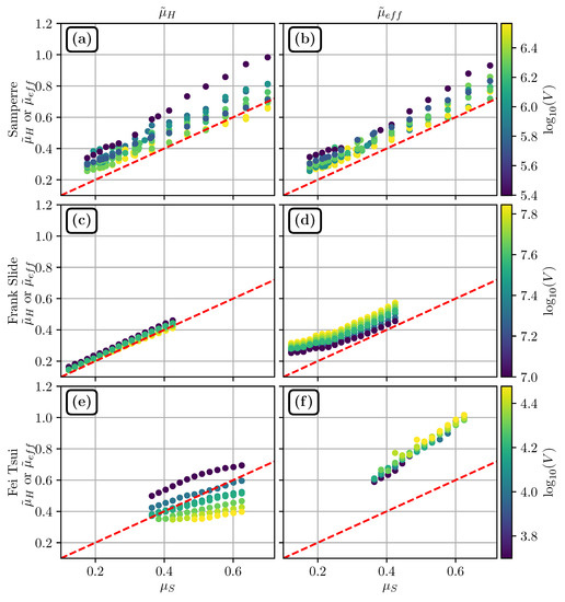
Figure 11.
and computed from simulations results, plotted against . (a) and (b) against and against (respectively) for the Samperre case study. (c) and (d) against and against (respectively) for the Frank Slide case study. (e) and (f) against and against (respectively) for the Fai Tsui debris slide case study. Color scale gives the volume (in logarithmic scale) of the simulation. The red dashed lines correspond to and .
As already discussed in the literature, e.g., [4,5,47,48], the Heim’s ratio can’t be considered as a good proxy for the real basal friction coefficient of the landslide. Indeed, the reduction of with increasing volumes results from real friction reduction (in the sense that a lower friction coefficient is needed to model larger landslide) but also from purely geometrical effects. This is illustrated in our simulations in the Samperre and Fei Tsui Road case studies: when the volume V is increased but remains constant, is reduced (see Figure 11a,e).
This should be supposedly corrected for with whose expression (2) was derived analytically to match [5]. However, though is almost constant for various volumes and a given in the Fei Tsui Road case study (Figure 11f), it increases with volume in the Frank Slide case study (Figure 11d), but on the contrary decreases with volume in the Samperre case study (Figure 11b). This may be explained by the fact that, for the Frank Slide case study, the increase of initial volume favors lateral spreading, such that in (2), the augmentation of the initial maximum thickness is not compensated by an augmentation of the travel distance along topography . The opposite happens in the Samperre case study, where the landslide is laterally confined in a narrow ravine.
These results highlight the complexity of defining simple mobility estimations that can be computed from landslide deposits and be used as proxys for the friction coefficient . In particular, the description of topography is not easy. The analytical development leading to the definition of in [5] was done for landslides on 1D planar surfaces (that is, on a 1D topography given by a graph ). Thus, it does not take into account lateral spreading that can limit travel distance: it has been observed empirically that lateral confinement increases travel distances [8,31]. Besides, the propagation of landslides on complex topographies with non constant slope is not predicted either. In [5], the formal expression of is extended empirically to non constant slopes by considering the average slope along the landslide path. As discussed previously, it proved to yield conclusive results at the scale of the database, but it may not be precise enough when considering forward prediction in a specific case study.
Indeed, when we try using directly to estimate travel distances (that is, with the function ), we get somehow unstable results. Though the estimation is good for the Samperre Cliff (Figure 7e), high uncertainties are obtained for the Frank Slide case study. In the latter case, the dependence to volume seems also over-estimated in comparison with other estimations (Figure 9e). Finally for the Fei Tsui Road case study, the observed travel distance is over-estimated by 45%.
Thus, further investigations are needed to try and derive formulas relating landslides deposits and topography geometry to . This could be done by modeling the propagation of landslides on synthetic topographies with, for instance, a slope break or an exponential profiles, and analyze the correlations between and derived from simulations results, and .
Another possibility is to disregard empirical mobility estimations, and consider instead directly the friction coefficient needed to reproduce each event from a database of at least, typically, 30 landslides, which is necessary to evaluate correctly uncertainty. The resulting relation could be then used directly in the function derived from site-specific simulations. The systematic back-analysis of mapped landslides has been done for instance in [49,50] but with the Voellmy rheology. We could find only one example of such studies with the Coulomb rheology in [9], but for a small range of volumes (between 0 and 10,000 m) and 1D simulations (i.e., along profiles, not on real topographies). Note that the relation may depend on the numerical code used to derive it: although thin-layer models solve roughly similar equations, differences in equations (in particular related to the description of internal stress) and numerical implementations can affect the results. For instance, we found a best-fit friction coefficient for the Frank Slide, but is obtained in [51], and in [52]
In any case, a good estimation of is important, because it will influence the final estimation of travel distance, and in particular the dependence to volume.
4.3. Dependence between Travel Distance and Volume
In our final estimations of travel distance , the dependence to volume is measured by . It varies significantly depending on the methodology and on the case study. In empirical/numercial estimations, is increased in comparison with purely empirical estimations, all the more so as volumes are small. For instance in the Frank Slide case study, the exponent of empirical estimations and is 20% below the exponent of (where we set ). In the Fei Tsui Road case study, it is 75% below (see Table 2). This shows that does not model properly the influence of the initial volume on the final travel distance, particularly for small landslides.
The influence of initial volume on travel distance is indeed all the more important as we consider small landslides with limited travel distances. This is illustrated by comparing the exponents of V and in the function (see Table A1 and Appendix C). For the Fei Tsui Road case study, volumes variations represents 20% of the total variance of travel distances, the rest being attributed to variations of . For the Samperre and Frankslide case studies, this proportion drops down to 3.7% and 0.3%, respectively. This is not rendered in the empirical relations and , explaining why and under-estimate the dependance to volume in comparison with empirical/numerical estimations.
These observations also explain why, in the Fei Tsui Road case study, the dependence to volume are similar between the empirical/numerical estimations of travel distance and the purely numerical estimations where we use the back-analyzed value of . We have indeed or in the former estimations, and for , with a constant friction coefficient derived by back-analysis. In comparison, for the Frank Slide case study, the exponent in is less than half the exponent in , and . Indeed, in this case, the travel distance depends mainly on the friction coefficient , such that choosing a constant value of instead of a volume dependent value has more impact than in the Fei Tsui Road case study.
These results may seem contradictory with empirical power laws derived directly from landslide databases. The exponent varies between 0.25 and 0.39 in [4] and does not seem to depend on the range of volumes considered. In [5], for m, for m and for all volumes. One possible explanation to the difference between these values and the ones of our study is that, for the Frank Slide and Fei Tsui Road simulations, our initial unstable mass were constructed by simply scaling the heights of the documented landslide to obtain different volumes, without changing the scar geometry. Though it was shown that the initial scar geometry has little influence on the landslide runout [53], it may be worth investigating more realistic initial settings.
However, our empirical estimations and also display exponents significantly different, between 0.06 and 0.13, whereas for . The discrepancies in volume dependencies are thus not related only to numerical issues. It may rather be related to the fact that and are site-specific relations, while is not as it uses observations of V and on different topographies. In turn, it may be possible that aggregating the observations of landslides on various topographies yields an exponent close to 0.33, as predicted by analytical results for landslides propagating on constant slopes [5]. However, considering each topography separately may well result in topography-specific values for , different from 0.33.
5. Conclusions
In this work, we derived operational and site-specific power laws to predict the horizontal travel distance of a landslide from its volume V. Such simple relations are indeed of prior importance for landslide hazard assessment, in particular for crisis management when travel distance estimations must be provided quickly by practitioners. We have compared three methodologies to derive such power laws, using (i) a purely empirical approach, (ii) a database of simulations along with the back-analysis of a documented event, and (iii) combining an empirical estimation of mobility with simulations.
We show that:
- The best results, in terms of prediction uncertainty, are obtained with numerical estimations of travel distances, with friction coefficient deduced from back-analysis. The standard deviation of estimations is indeed less than half the standard deviation of empirical/numerical estimations, and less than 30% the standard deviation of purely empirical estimations. However, the uncertainty on the back-analysis results are asserted, to some extent, in a expert way. In turn, comparison with other methodologies should be done with caution.
- Combining numerical modeling with empirical estimations of and reduces the uncertainty of estimation by about 50%, in comparison with purely empirical estimations. The smallest uncertainties are obtained by using to estimate the simulation friction coefficient . However, setting or results, in 2 out of the 3 tested case studies, in an under-estimation of observed travel distances.
- When we relate the effective friction coefficient observed on real landslides, to the effective friction coefficient computed from simulations results, the resulting estimations of travel distance displays large uncertainties (even larger than empirical estimates) and/or over-estimates observations. This could be explained by the fact that the analytic expression of and was derived for constant slopes, such that their definition on complex topographies is not straight-forward.
- Numerical simulations allow to better characterize the respective influence of initial volume and physical mobility (as measured with ) on the final travel distance, for a given topography. We show that for large landslide (i.e., for volumes m), the travel distance depends mainly on , while for small landslide (i.e., for volumes m) the initial volume V has a more prominent role. This is not rendered in empirical estimations of travel distances, for which the dependence of travel distance to volume is under-estimated, all the more so as small volumes are considered.
The milestone of our work is the construction of a simulation database, where various landslide volumes, collapse geometries and mobilities are tested. The definition of the initial unstable masses can be time consuming, especially when little information is available to constrain collapse geometries. This aspect may be the main practical difficulty to tackle in the perspective of using our methodology for operational hazard assessment, especially in a regulatory framework. Indeed, though the statistical analysis of results must be interpreted with caution, its implementation can be automated to a large degree. In comparison, the methodology for constructing initial geometries relies, at least to some extent, on expert judgment. It must be easy enough to be reproducible and applied in a reasonable time, but must also provide realistic collapse scenarios realistic enough. Further work, including applications to other case studies, is needed to better constrain the right balance between these two requirements. In any case, our study proves the relevance of using numerical simulations to improve empirical estimations of travel distances for operational use.
In this work, we have used only power laws which are easy to manipulate, but other non-parametric models, such as the General Additive Models, e.g., [54], could be used when linear regression models are not valid. Further research should also focus on the estimation of the friction coefficient to be used in simulations. This could be done by systematic back-analysis of a landslide database, and/or by adapting the definition of landslide mobility indicators, such as , to take into account the topography more precisely. However, we may expect that significant uncertainties will remain, as a result of the partial knowledge we have in practice of the process at stake during the landslide propagation. Thus, expert judgments are valuable to assess the representativeness of results. The selection, evaluation and aggregation of such judgments, e.g., [55] could also help constrain the estimation of runout.
To conclude, let’s note that the information in our simulation databases are greatly simplified for the purpose of this study, as we focused only on the estimation of travel distances. However, we could also extract thicknesses and dynamic pressure maps for various volumes as done for instance in tsunami hazard assessment [56]. The quantification of spatial uncertainty is however difficult and requires tools more complex than our simple power laws.
Supplementary Materials
The following are available online at https://www.mdpi.com/2076-3263/10/11/424/s1.
Author Contributions
Conceptualization, Methodology and Validation, M.P., A.M., G.G., C.L., Y.T., J.R., A.L.; Formal Analysis, M.P., J.R., Investigation and Visualization M.P.; Resources, C.L., Y.T., A.L.; Data Curation, M.P., C.L., Y.T., A.L.; Writing—Original Draft Preparation, M.P.; Writing—Review & Editing, M.P., A.M., G.G., C.L., Y.T., J.R., A.L.; Supervision, Project Administration, and Funding Acquisition A.M., G.G., C.L., Y.T. All authors have read and agreed to the published version of the manuscript.
Funding
This research was funded by the French Ministère de la Transtition Ecologique et Solidaire (MTES), the BRGM and the European Research Council grant number ERC-CG-2013-PE10-617472 SLIDEQUAKES. This study contributes to the Université de Paris ANR-18-IDEX-0001 IdEx initiative.
Acknowledgments
Numerical computations were performed on the S-CAPAD platform, IPGP, France. This is IPGP contribution 4168. We thank the staff of OVSM-IPGP, BRGM Guadeloupe and BRGM Martinique for their contribution to the work on the Prêcheur river and the staff of the OVS (IPGP) for insightful discussions. DEAL Martinique funded the LIDAR acquisition of the Prêcheur topography in August 2018. The Joint Technical Committee on Natural Slopes and Landslides (JTC1) of the Federation of International Geo-engineering Societies (FedIGS) provided the data for the Frank Slide and the Fei Tsui debris slide. We thank Bastien Colas for his help recovering the landslide database from [3], as well as Frank Ou and two anonymous reviewers for their comments and suggestions.
Conflicts of Interest
The authors declare no conflict of interest.
Abbreviations
The following abbreviations are used in this manuscript:
| DEM | Digital Elevation Model |
| OLS | Ordinary Least Squares |
Appendix A. Simulation Database for the Samperre Cliff Case Study
The Samperre cliff destabilizations occurred in several successive steps, such that the available topographic surveys of March 2010, July 2010, January 2018 and August 2018 do not allow an exact reconstruction of the destabilized volumes. The volume of the major 2009 cliff collapse was estimated to m [39], but the scar geometry is unknown. Thus, we reconstruct empirically the initial mass by scaling the difference between the March and July 2010 DEMs (before and after another major destabilization episode) to obtain a m, which is the estimated volume involved in the August 2009 collapse. The avalanche propagation is then modeled on the July 2010 DEM. Another documented destabilization took place in January 2018. We estimate its volume at m from the difference between the January 2018 DEM, and a synthetic reconstruction of the cliff in 2017 (constrained by the cliff rim as observed on ortho-photographs). The resulting mass is propagated on the January 2018 DEM. We generate other initial geometries as follows:
- By taking the difference between the March and July 2010 DEMs. The resulting m mass is propagated on the July 2010 DEM. It is also scaled uniformly to consider a smaller volumes (250,000 m).
- By taking the difference between the July 2010 and January 2018 DEMs, resulting in a m initial mass that is released on the Januray 2018 DEM. Three intermediate synthetic topographies are also considered, yielding three other volumes ( m, m and m).
- By considering two possible future destabilizations on the eastern and northern side of the cliff ( m and m, respectively). The resulting avalanche is propagated on the August 2018 DEM.
Thus, we run simulations for a total of 10 initial volumes/geometries. Friction coefficients are chosen between and every 1°, and every up to . This results in a total of 154 simulations. Note that the different DEMs on which the simulations are run differ near the cliff as a result of its progressive retreat, but the Samperre river, where the avalanches propagate, did not significantly vary. The DEMs are all re-interpolated to 5 m.
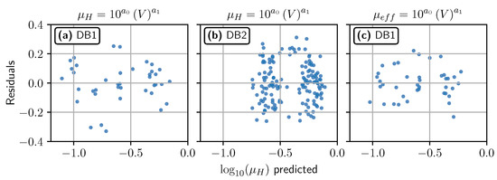
Figure A1.
Residuals VS predicted values for the different power laws deduced from empirical databases. The axis scale is logarithmic. (a) , with DB1. (b) , with DB2. (c) , with DB1.
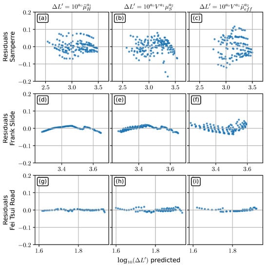
Figure A2.
Residuals VS predicted values for the different power laws deduced for each case study. The axis scale is logarithmic. Each line refers to a case study, and each column to a law. (a–c): , and , respectively for the Samperre cliff case study. (d–f): , and , respectively for the Frank Slide case study. (g–i): , and , respectively for the Fei Tsui Road debris slide case study.

Table A1.
Results of the intermediate power laws. We give the coefficients along with the 95% confidence interval. We also indicate the adjusted and the p-values of the Harvey-Collier test (HC, linearity hypothesis), of the Jarque-bera test (J-B, normality of residuals hypothesis) and of the Breush-Pagan test (B-P, homoscedasticity hypothesis). Low p-values (typically, less than 0.05) indicate that the hypothesis is not verified. The Variance Inflation Factor (VIF) measures colinearity between and .
| B-P | J-B | R2 | VIF | |||||
|---|---|---|---|---|---|---|---|---|
| DB1 | 0.0691 ± 0.1107 | −0.0875 ± 0.0135 | n.a. | 0.23 | 0.29 | 0.82 | n.a. | |
| DB2 | 0.0287 ± 0.0530 | −0.0889 ± 0.0099 | n.a. | 0.20 | 0.18 | 0.68 | n.a. | |
| DB1 | −0.0335 ± 0.0872 | −0.0739 ± 0.0105 | n.a. | 0.98 | 0.83 | 0.84 | n.a. | |
| Samperre | 2.5291 ± 0.0128 | −1.6113 ± 0.0328 | n.a. | 0.07 | 0.01 | 0.98 | n.a. | |
| Frank Slide | 3.0274 ± 0.0069 | −0.7345 ± 0.0120 | n.a. | 0.01 | 0.00 | 0.99 | n.a. | |
| Fei Tsui Road | 1.4496 ± 0.0031 | −1.0543 ± 0.0089 | n.a. | 0.99 | 0.00 | 1.00 | n.a. | |
| Samperre | 1.1697 ± 0.1061 | 0.2275 ± 0.0172 | −1.1557 ± 0.0317 | 0.40 | 0.00 | 0.97 | 1.00 | |
| Frank Slide | 2.7682 ± 0.0566 | 0.0374 ± 0.0075 | −0.6460 ± 0.0119 | 0.04 | 0.05 | 0.99 | 1.00 | |
| Fei Tsui Road | 0.2373 ± 0.0347 | 0.3346 ± 0.0078 | −0.6103 ± 0.0266 | 0.78 | 0.14 | 0.99 | 1.03 | |
| Samperre | 1.7719 ± 0.1751 | 0.1287 ± 0.0293 | −1.5085 ± 0.0904 | 0.00 | 0.12 | 0.91 | 1.05 | |
| Frank Slide | 1.4650 ± 0.1070 | 0.1872 ± 0.0133 | −1.2926 ± 0.0446 | 0.01 | 0.30 | 0.97 | 1.08 | |
| Fei Tsui Road | 0.3313 ± 0.0406 | 0.3407 ± 0.0097 | −0.6919 ± 0.0442 | 0.02 | 0.12 | 0.99 | 1.01 |
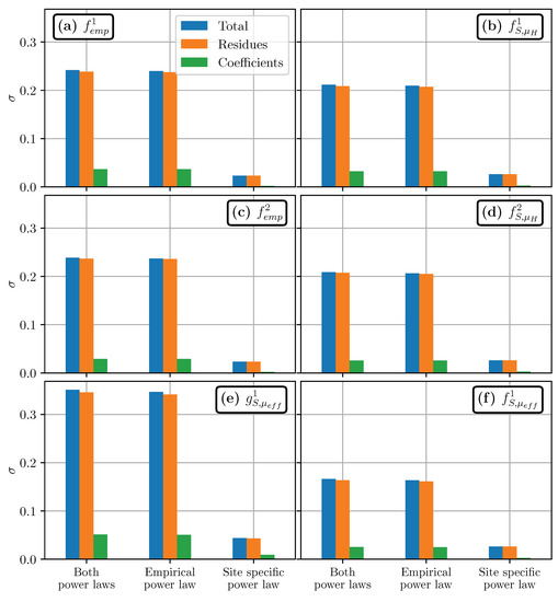
Figure A3.
Uncertainty in travel distance estimation for the Frank Slide cliff case study. (a–f), and symbology are the same as for Figure 8.
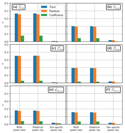
Figure A4.
Uncertainty in travel distance estimation for the Fei Tsui Road cliff case study. (a–f), and symbology are the same as for Figure 8.
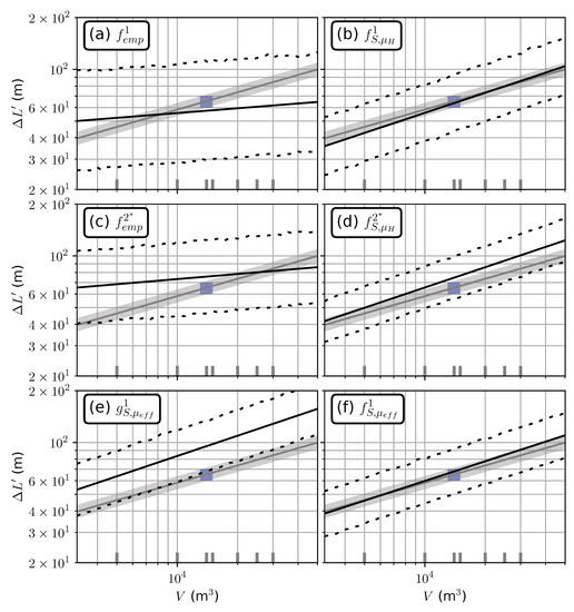
Figure A5.
Travel distance estimated from volume for the Fei Tsui Road case study, and a variation of DB2 with only debris flows, debris avalanches and debris slides. The corresponding travel distance estimations are marked with the super-script . Notations are otherwise the same as in the main body of the article. Green and blue rectangles: estimations of volumes and travel distances for the 2009 and 2018 collapses, respectively. Grey line: Numerical estimation from back-analysis (), with . The grey area is the upper and lower limits of the 95% prediction intervals derived for . (a) Estimation with . (b) Estimation with . (c) Estimation with . (d) Estimation with . (e) Estimation with . (f) Estimation with . Black lines are direct estimates, dashed lines give the 95% prediction interval.
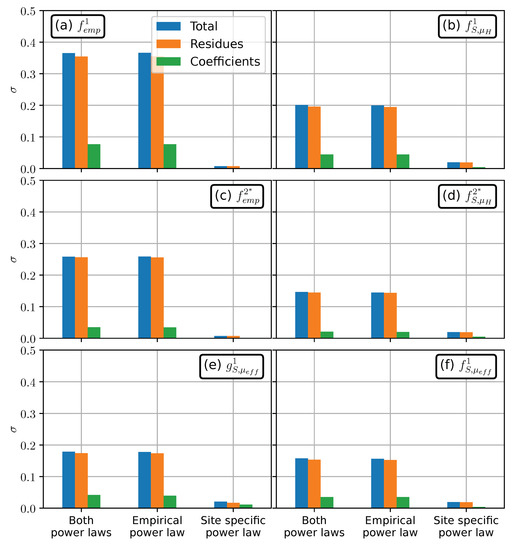
Figure A6.
Uncertainty in travel distance estimation for the Fei Tsui Road cliff case study, and a variation of DB2 with only debris flows, debris avalanches and debris slides. The corresponding travel distance estimations are marked with the super-script . Notations are otherwise the same as in the main body of the article. (a–f), and symbology are the same as for Figure 8.
Appendix B. Power Law Derivation and Uncertainty Estimation
We use the statsmodel python package [57] to derive power laws, through Ordinary Least Square (OLS) linear or multi-linear regressions [58]. Fitting a power law is indeed equivalent to fitting a linear model For , and , a first OLS regression is carried out and outliers (points whose residue have a Student p-value lower than 0.025) are removed. A new OLS regression is then carried out. The quality of the linear regression is primarily given by the coefficients confidence interval and the adjusted . Note that a rigorous estimation of uncertainty should take into account both the dispersion between the data and the best-fit, and the uncertainty on the best-fit linear model coefficients. For instance, let’s assume we have set of data (e.g., observed volumes) and (e.g., travel distances), for which we want to derive a linear model of the form:
where the are the residues. Then the OLS regression will find and such that is minimal. If the residues have a normal distribution that does not depend on x or y, and are centered on 0, then for a new value , we can derive a confidence interval around the best-fit estimate:
where is the standard deviation of the residuals and is a coefficient that depends on the number n of observations and on the level of confidence. It is derived from the Student law with degree of freedom. However, such an interval does not take into account the uncertainty on the estimations and and thus has no real statistical meaning.
On the contrary, if we disregard the uncertainty on residues but consider the uncertainty on coefficients, we derive the confidence interval:
where is the mean of the , and their estimated variance. This interval has a given probability (e.g., 95%) of containing , where a and b are the "real" coefficients (remember the OLS regression provides only estimations and ). Note that the interval is all the more large as is further away from the samples .
If we now combine the uncertainty on the coefficients estimation and the dispersion of the data around the best fit, we get the prediction interval:
The resulting interval has a given probability of containing the real value estimated with the real coefficient a and b and taking into account a residue that follows a centered normal law with standard deviation .
The previous formulas are derived for simple linear regressions but can be extended to multi-linear regressions. However, the derivation of confidence and prediction intervals for nested linear fits (that is, when the prediction of a linear model is used as input of another linear model) is not straight-forward. Thus, we derive them numerically by computing 1,000 4,000 estimations: the coefficients and/or the residues of the successive linear models are drawn randomly following normal laws whose parameters are given by the OLS regression results. To get for instance a 95% interval, we then identify the 2.5th and 97.5th percentiles.
If we consider for instance the empirical estimation of travel distance , it uses successively two power laws:
where , , , are coefficients estimated by the regression and and are residues. The total uncertainty (i.e., prediction interval) for a given volume is obtained with random draws on , , , , and . We can also consider only the best-fit values of the power laws coefficients and draw only and , or to the contrary disregard dispersion and draw only , , and . Finally we can distinguish between the uncertainties specific to each power law by drawing only , and , or only , and .
The previous methodology can be deemed to represent correctly real uncertainties only if certain conditions are met:
- There is indeed a linear relation between the input (x) and output values (y). This can be verified with the Harvey-Collier test that evaluates to what extent the slope ofthe linear regression changes when data points are recursively added. In practice, we could not implement this test in a satisfactory manner, because results proved to depend strongly on the order in which points were added. Thus, we evaluate linearity graphically with the graph of residuals: if they have concave or convexe shapes, then the hypothesis of linearity can be questionned (Figure A1 and Figure A2).
- The residuals have a normal distribution. This is can be verified with the Jarque-Bera test.
- The residuals are homoscedastic: they do not depend on the value y predicted by the linear model. In other words, the dispersion between the linear fit and the predicted value is the same for all predicted values. Graphically, this means the scatter plot of residuals against predicted value does not have a cone shape. This is quantitatively assessed with the Breush-Pagan test.
- For multi-linear regressions, the explanatory input variables are not linearly related. This can be assessed by computing the Variance Inflation Factor (VIF) for each associated coefficient. High VIF (typically above 5 or 10) indicate strong linear correlations
Appendix C. Propagation of Uncertainty in Power Laws
Let’s consider a power law that was derived with OLS regression.
We want to quantify how uncertainties on x and y will impact the estimation of z. In a first approximation (that is, without considering the uncertainty on the estimation of a, c and c), this can be done by considering the first order development:
that stands true if . In turn, if we consider small relative variations and of, respectively, and , we compute the first order approximation:
where . If we now assume and follow some uncorrelated random laws with known variances and , the ratio of the variance of the error on z linked to error on x, over the total variance of the error on z, is:
If we further assume , we get:
Similarly, we derive:
References
- Corominas, J.; van Westen, C.; Frattini, P.; Cascini, L.; Malet, J.P.; Fotopoulou, S.; Catani, F.; Van Den Eeckhaut, M.; Mavrouli, O.; Agliardi, F.; et al. Recommendations for the quantitative analysis of landslide risk. Bull. Eng. Geol. Environ. 2014, 73, 209–263. [Google Scholar] [CrossRef]
- Thiery, Y.; Vandromme, R.; Maquaire, O.; Bernardie, S. Landslide Susceptibility Assessment by EPBM (Expert Physically Based Model): Strategy of Calibration in Complex Environment. In Advancing Culture of Living with Landslides; Mikos, M., Tiwari, B., Yin, Y., Sassa, K., Eds.; Springer International Publishing: Cham, Switzerland, 2017; pp. 917–926. [Google Scholar]
- Corominas, J. The angle of reach as a mobility index for small and large landslides. Can. Geotech. J. 1996, 33, 260–271. [Google Scholar] [CrossRef]
- Legros, F. The mobility of long-runout landslides. Eng. Geol. 2002, 63, 301–331. [Google Scholar] [CrossRef]
- Lucas, A.; Mangeney, A.; Ampuero, J.P. Frictional velocity-weakening in landslides on Earth and on other planetary bodies. Nat. Commun. 2014, 5. [Google Scholar] [CrossRef]
- Zhan, W.; Fan, X.; Huang, R.; Pei, X.; Xu, Q.; Li, W. Empirical prediction for travel distance of channelized rock avalanches in the Wenchuan earthquake area. Nat. Hazards Earth Syst. Sci. 2017, 17, 833–844. [Google Scholar] [CrossRef]
- Mitchell, A.; McDougall, S.; Whittall, J.; Brideau, M.A.; McClarty, D. New empirical-statistical tools for the analysis of rock avalanche runout. In Proceedings of the 7th Canadian Geohazards Conference, Canmore, AB, Canada, 3–6 June 2018; p. 7. [Google Scholar]
- Strom, A.; Abdrakhmatov, K. Quantitative Relationships of Central Asian Bedrock Landslide Parameters. In Rockslides and Rock Avalanches of Central Asia; Elsevier: Amsterdam, The Netherlands, 2018; pp. 335–347. [Google Scholar]
- Brideau, M.A.; Stead, D.; Millard, T.H.; Ward, B.C. Field characterisation and numerical modelling of debris avalanche runout on Vancouver Island, British Columbia, Canada. Landslides 2019, 16, 875–891. [Google Scholar] [CrossRef]
- Hungr, O.; Corominas, J.; Eberhardt, E. Estimating landslide motion mechanism, travel distance and velocity. Landslide Risk Manag. 2005, 1, 99–128. [Google Scholar]
- Mangeney, A.; Heinrich, P.; Roche, R. Analytical Solution for Testing Debris Avalanche Numerical Models. Pure Appl. Geophys. 2000, 157, 1081–1096. [Google Scholar] [CrossRef]
- Wichmann, W.; Becht, M. Modelling of geomorphological processes in an alpine catchment. In GeoDynamics, Chapter: 12; Foody, A., Wu, D., Eds.; CRC Press: Boca Raton, FL, USA, 2005. [Google Scholar]
- Horton, P.; Jaboyedoff, M.; Rudaz, B.; Zimmermann, M. Flow-R, a model for susceptibility mapping of debris flows and other gravitational hazards at a regional scale. Nat. Hazards Earth Syst. Sci. 2013, 13, 869–885. [Google Scholar] [CrossRef]
- Leonardi, A.; Wittel, F.K.; Mendoza, M.; Herrmann, H.J. Coupled DEM-LBM method for the free-surface simulation of heterogeneous suspensions. Comput. Part. Mech. 2014, 1, 3–13. [Google Scholar] [CrossRef]
- Prime, N.; Dufour, F.; Darve, F. Solid-fluid transition modelling in geomaterials and application to a mudflow interacting with an obstacle. Int. J. Numer. Anal. Methods Geomech. 2014, 38, 1341–1361. [Google Scholar] [CrossRef]
- Hu, M.; Liu, M.B.; Xie, M.W.; Liu, G.R. Three-dimensional run-out analysis and prediction of flow-like landslides using smoothed particle hydrodynamics. Environ. Earth Sci. 2015, 73, 1629–1640. [Google Scholar] [CrossRef]
- Salm, B. Flow, flow transition and runout distances of flowing avalanches. Ann. Glaciol. 1993, 18, 221–226. [Google Scholar] [CrossRef]
- McDougall, S. 2014 Canadian Geotechnical Colloquium: Landslide runout analysis—current practice and challenges. Can. Geotech. J. 2017, 54, 605–620. [Google Scholar] [CrossRef]
- Pastor, M.; Quecedo, M.; González, E.; Herreros, M.I.; Merodo, J.A.F.; Mira, P. Simple Approximation to Bottom Friction for Bingham Fluid Depth Integrated Models. J. Hydraul. Eng. 2004, 130, 149–155. [Google Scholar] [CrossRef]
- McDougall, S.; Hungr, O. Dynamic modelling of entrainment in rapid landslides. Can. Geotech. J. 2005, 42, 1437–1448. [Google Scholar] [CrossRef]
- Pirulli, M.; Pastor, M. Numerical study on the entrainment of bed material into rapid landslides. Géotechnique 2012, 62, 959–972. [Google Scholar] [CrossRef]
- Iverson, R.M. Debris flows: Behaviour and hazard assessment. Geol. Today 2014, 30, 15–20. [Google Scholar] [CrossRef]
- Bouchut, F.; Fernández-Nieto, E.; Mangeney, A.; Narbona-Reina, G. A two-phase shallow debris flow model with energy balance. Math. Model. Numer. Anal. 2015, 49, 101–140. [Google Scholar] [CrossRef]
- Bouchut, F.; Fernández-Nieto, E.D.; Mangeney, A.; Narbona-Reina, G. A two-phase two-layer model for fluidized granular flows with dilatancy effects. J. Fluid Mech. 2016, 801, 166–221. [Google Scholar] [CrossRef]
- Pudasaini, S.P.; Mergili, M. A Multi-Phase Mass Flow Model. J. Geophys. Res. Earth Surf. 2019, 124, 2920–2942. [Google Scholar] [CrossRef]
- Iverson, R.M.; Denlinger, R.P. Flow of variably fluidized granular masses across three-dimensional terrain: 1. Coulomb mixture theory. J. Geophys. Res. Solid Earth 2001, 106, 537–552. [Google Scholar] [CrossRef]
- Hussin, H.Y.; Quan Luna, B.; van Westen, C.J.; Christen, M.; Malet, J.P.; van Asch, T.W.J. Parameterization of a numerical 2-D debris flow model with entrainment: A case study of the Faucon catchment, Southern French Alps. Nat. Hazards Earth Syst. Sci. 2012, 12, 3075–3090. [Google Scholar] [CrossRef]
- Mergili, M.; Frank, B.; Fischer, J.T.; Huggel, C.; Pudasaini, S.P. Computational experiments on the 1962 and 1970 landslide events at Huascarán (Peru) with r.avaflow: Lessons learned for predictive mass flow simulations. Geomorphology 2018, 322, 15–28. [Google Scholar] [CrossRef]
- Peruzzetto, M.; Komorowski, J.C.; Friant, A.L.; Rosas-Carbajal, M.; Mangeney, A.; Legendre, Y. Modeling of partial dome collapse of La Soufrière of Guadeloupe volcano: Implications for hazard assessment and monitoring. Sci. Rep. 2019, 9, 1–15. [Google Scholar] [CrossRef] [PubMed]
- Rohmer, J.; Foerster, E. Global sensitivity analysis of large-scale numerical landslide models based on Gaussian-Process meta-modeling. Comput. Geosci. 2011, 37, 917–927. [Google Scholar] [CrossRef]
- Mitchell, A.; McDougall, S.; Nolde, N.; Brideau, M.A.; Whittall, J.; Aaron, J.B. Rock avalanche runout prediction using stochastic analysis of a regional dataset. Landslides 2019. [Google Scholar] [CrossRef]
- Mangeney-Castelnau, A.; Bouchut, F.; Vilotte, J.P.; Lajeunesse, E.; Aubertin, A.; Pirulli, M. On the use of Saint Venant equations to simulate the spreading of a granular mass: Numerical simulation of granular spreading. J. Geophys. Res. Solid Earth 2005, 110. [Google Scholar] [CrossRef]
- Bouchut, F.; Westdickenberg, M. Gravity driven shallow water models for arbitrary topography. Commun. Math. Sci. 2004, 2, 359–389. [Google Scholar] [CrossRef]
- Mangeney, A.; Bouchut, F.; Thomas, N.; Vilotte, J.P.; Bristeau, M.O. Numerical modeling of self-channeling granular flows and of their levee-channel deposits. J. Geophys. Res. 2007, 112. [Google Scholar] [CrossRef]
- Lucas, A.; Mangeney, A.; Bouchut, F.; Bristeau, M.O.; Mège, D. Benchmarking Exercises for Granual Flows; Ho & Li: Hong Kong, China, 2007. [Google Scholar]
- Moretti, L.; Allstadt, K.; Mangeney, A.; Capdeville, Y.; Stutzmann, E.; Bouchut, F. Numerical modeling of the Mount Meager landslide constrained by its force history derived from seismic data. J. Geophys. Res. Solid Earth 2015, 120, 2579–2599. [Google Scholar] [CrossRef]
- Yamada, M.; Mangeney, A.; Matsushi, Y.; Matsuzawa, T. Estimation of dynamic friction and movement history of large landslides. Landslides 2018, 15, 1963–1974. [Google Scholar] [CrossRef]
- Moretti, L.; Mangeney, A.; Walter, F.; Capdeville, Y.; Bodin, T.; Stutzmann, E.; Le Friant, A. Constraining landslide characteristics with Bayesian inversion of field and seismic data. Geophys. J. Int. 2020, 221, 1341–1348. [Google Scholar] [CrossRef]
- Clouard, V.; Athanase, J.E.; Aubaud, C. Physical characteristics and triggering mechanisms of the 2009-2010 landslide crisis at Montagne Pelee volcano, Martinique: Implication for erosional processes and debris-flow hazards. Bull. Soc. Geol. Fr. 2013, 184, 155–164. [Google Scholar] [CrossRef]
- Nachbaur, A.; Legendre, Y.; Lombard, M.; Dewez, T. Caractérisation Géologique et Identification des Mécanismes D’instabilité de la Falaise Samperre; Rapport Final RP-68564-FR; BRGM: Paris, France, 2019. [Google Scholar]
- Quefféléan, Y. Mission d’expertise ONF-RTM sur les Lahars du Prêcheur; Technical Report; ONF-RTM: Paris, France, 2018. [Google Scholar]
- Benko, B.; Stead, D. The Frank slide: A reexamination of the failure mechanism. Can. Geotech. J. 1998, 35, 13. [Google Scholar] [CrossRef]
- GEO. Report on the Fei Tsui Road Landslide of August 1995, Volume 2; Findings of the Landslide Investigation, Geotechnical Engineering office: Hong-Kong, China, 1996. [Google Scholar]
- Knill, J. Report on the Fei Tsui Road Landslide of August 1995, Volume 1; Independent Review of the Investigation by the Geotechnical Engineering Office; Geotechnical Engineering Office: Hong-Kong, China, 1996. [Google Scholar]
- Aubaud, C.; Athanase, J.E.; Clouard, V.; Barras, A.V.; Sedan, O. A review of historical lahars, floods, and landslides in the Precheur river catchment (Montagne Pelee volcano, Martinique island, Lesser Antilles). Bull. Soc. Geol. Fr. 2013, 184, 137–154. [Google Scholar] [CrossRef]
- Hungr, O.; Morgenstern, N.; Wong, H. Review of benchmarking exercise on landslide debris runout and mobility modelling. In 2007 International Forum on Landdslide Disaster Management; Ho & Li: Hong-Kong, China, 2007. [Google Scholar]
- Lajeunesse, E.; Quantin, C.; Allemand, P.; Delacourt, C. New insights on the runout of large landslides in the Valles-Marineris canyons, Mars. Geophys. Res. Lett. 2006, 33, L04403. [Google Scholar] [CrossRef]
- Finlay, P.J.; Mostyn, G.R.; Fell, R. Landslide risk assessment: Prediction of travel distance. Can. Geotech. J. 1999, 36, 7. [Google Scholar] [CrossRef]
- Aaron, J.; McDougall, S. Rock avalanche mobility: The role of path material. Eng. Geol. 2019. [Google Scholar] [CrossRef]
- Zimmermann, F.; McArdell, B.W.; Rickli, C.; Scheidl, C. 2D Runout Modelling of Hillslope Debris Flows, Based on Well-Documented Events in Switzerland. Geosciences 2020, 10, 70. [Google Scholar] [CrossRef]
- Pirulli, M.; Mangeney, A. Results of Back-Analysis of the Propagation of Rock Avalanches as a Function of the Assumed Rheology. Rock Mech. Rock Eng. 2008, 41, 59–84. [Google Scholar] [CrossRef]
- Hungr, O.; Evans, S.G. Rock avalanche run out prediction using a dynamic model. In Proceedings of the 7th International Symposium on Landslides, Trondheim, Norway, 17–21 June 1996; pp. 233–238. [Google Scholar]
- Lucas, A.; Mangeney, A.; Mège, D.; Bouchut, F. Influence of the scar geometry on landslide dynamics and deposits: Application to Martian landslides. J. Geophys. Res. 2011, 116. [Google Scholar] [CrossRef]
- Wood, S.N. Generalized Additive Models: An Introduction with R, 2nd ed.; Chapman and Hall/CRC: Boca Raton, FL, USA, 2017. [Google Scholar]
- Hathout, M.; Vuillet, M.; Carvajal, C.; Peyras, L.; Diab, Y. Expert judgments calibration and combination for assessment of river levee failure probability. Reliab. Eng. Syst. Saf. 2019, 188, 377–392. [Google Scholar] [CrossRef]
- Aniel-Quiroga, I.; Álvarez Gómez, J.A.; González, M.; Martínez Sánchez, J.; Parro, L.M.; Aguirre-Ayerbe, I.; Fernández, F.; Medina, R.; Al-Yahyai, S. Tsunami Hazard assessment and Scenarios Database for the Tsunami Warning System for the coast of Oman. Prepr. Sea, Ocean. Coast. Hazards 2018. [Google Scholar] [CrossRef]
- Seabold, S.; Perktold, J. statsmodels: Econometric and statistical modeling with python. In Proceedings of the 9th Python in Science Conference, Austin, TX, USA, 28 June–3 July 2010. [Google Scholar]
- Kraemer, W.; Sonnberger, H. The Linear Regression Model Under Test; Physica-Verlag: Heidelberg, Germany, 1986. [Google Scholar]
Publisher’s Note: MDPI stays neutral with regard to jurisdictional claims in published maps and institutional affiliations. |
© 2020 by the authors. Licensee MDPI, Basel, Switzerland. This article is an open access article distributed under the terms and conditions of the Creative Commons Attribution (CC BY) license (http://creativecommons.org/licenses/by/4.0/).