Article

Habitat Shifts in the Pacific Saury (Cololabis saira) Population in the High Seas of the North Pacific Under Medium-to-Long-Term Climate Scenarios Based on Vessel Position Data and Ensemble Species Distribution Models

1
Key Laboratory of Oceanic and Polar Fisheries, East China Sea Fisheries Research Institute, Chinese Academy of Fishery Sciences, Shanghai 200090, China
2
College of Navigation and Ship Engineering, Dalian Ocean University, Dalian 116023, China
3
College of Marine Living Resource Sciences and Management, Shanghai Ocean University, Shanghai 201306, China
4
School of Geography and Ocean Science, Nanjing University, Nanjing 210023, China
5
School of Ecology and Environment, Anhui Normal University, Wuhu 241000, China
6
Wenchang Innovation Research Center, East China Sea Fisheries Research Institute, Chinese Academy of Fishery Sciences, Wenchang 571343, China
*
Authors to whom correspondence should be addressed.
These authors contributed equally to this work.
Animals 2025, 15(19), 2828; https://doi.org/10.3390/ani15192828
Submission received: 20 August 2025 / Revised: 23 September 2025 / Accepted: 25 September 2025 / Published: 28 September 2025
(This article belongs to the Special Issue Global Fisheries Resources, Fisheries, and Carbon-Sink Fisheries)

Abstract

Simple Summary

The Pacific saury is a commercially important fish in the North Pacific Ocean that is facing threats from climate change. To understand how its habitat might change in the future, we used a novel approach that combined high-resolution satellite tracking data from fishing vessels with advanced computer models. Our highly accurate model showed that sea surface temperature and the availability of food (measured as chlorophyll-a) are the most critical factors determining where the saury live. Our projections for the future are concerning. Under a high-emission scenario, the saury’s prime habitat is predicted to shrink by over 94% by the year 2100. Furthermore, the entire population is expected to shift its center of gravity more than 400 km to the northeast. These changes could create a “mismatch” in the food web, as predators may not be able to follow the saury’s rapid move. This study provides a crucial scientific tool for international fisheries managers, like the North Pacific Fisheries Commission, to develop proactive strategies to manage this vital resource in a changing climate.

Abstract

Global climate change poses a significant management challenge for vital transboundary resources like the Pacific saury (Cololabis saira). To address this, we developed an innovative framework that uses high-resolution Automatic Identification System (AIS) data and deep learning to define species distribution, which then informs a robust Ensemble Species Distribution Model (ESDM). The model (TSS > 0.89, AUC > 0.97) identifies sea surface temperature (SST) and chlorophyll-a (CHL) as key habitat drivers. Projections under future climate scenarios reveal two critical threats: (1) a continuous northeastward migration of the habitat’s centroid, exceeding 400 km by 2100 under a high-emission SSP5-8.5 scenario, and (2) a drastic contraction of highly suitable habitat (suitability > 0.8), shrinking by up to 94% under the high-emission SSP3-7.0 scenario. By directly linking key oceanographic features to these climate-driven risks, this study delivers an essential scientific decision-support tool for management bodies like the North Pacific Fisheries Commission (NPFC) to develop climate-adaptive strategies.

1. Introduction

Global climate change is profoundly reshaping the North Pacific Ocean, a region now considered a hotspot for rapid warming and acidification. Anomalous high-temperature events, such as the “The Blob” marine heatwave [1], intensify ocean stratification. This process hinders the vertical transport of deep-water nutrients to the surface, leading to a large-scale restructuring of primary productivity patterns (e.g., Chlorophyll-a concentrations) [2], which directly disrupts the foraging grounds of key species. These environmental shifts compel marine species to migrate poleward, disrupting established food webs. This impact is already evident in major commercial fisheries, with well-documented declines in iconic populations such as Pacific salmon (Oncorhynchus spp.) and Pacific cod (Gadus macrocephalus) [3,4,5].In this context, the Pacific saury (Cololabis saira) serves as an ideal case study. As a short-lived, migratory pelagic fish, it forms a crucial link in the food web [6], preying on zooplankton while serving as core prey for higher-trophic-level organisms such as tuna, squid, seabirds, and marine mammals. The species supports a major distant-water fishery involving multiple countries, including China, Japan, Russia, and South Korea [7,8], and is a priority for management by the North Pacific Fisheries Commission (NPFC). However, its distribution has become increasingly unpredictable, rendering traditional, experience-dependent management approaches inadequate.
To accurately forecast the saury’s future trajectory, it is essential to move beyond the limitations of traditional fishery logbooks, which often lack spatiotemporal resolution and accuracy [3]. High-resolution Automatic Identification System (AIS) data, by contrast, offering an unprecedentedly accurate source of species presence data [9,10]. While obtaining multi-national AIS data is challenging, this study utilizes a comprehensive dataset from the Chinese distant-water fleet. This fleet was selected as a robust proxy because its extensive operational range covers the main high seas fishing grounds, and its activities—representing a substantial portion of the total high-seas catch—provide a reliable reflection of the species’ overall distribution. Despite this progress, a systematic forecast of saury habitat changes under long-term climate scenarios remains a critical gap [11], a need made more urgent by the species’ recent assessment as being in an overfished state. Therefore, this study pioneers an integrated framework that combines deep learning with an Ensemble Species Distribution Model (ESDM) to quantify the key drivers of saury distribution and predict how its habitat will contract and shift [12,13]. The aim is to provide a strong scientific basis for the adaptive management and sustainable utilization of this critical resource.

2. Materials and Methods

2.1. Data Sources

2.1.1. Vessel Position Data

Given that obtaining multi-national vessel position data is often challenging due to data sensitivity, this study utilized a comprehensive AIS dataset from the Chinese distant-water stick-held dip net fleet from 2019 to 2024. This technology provides unprecedented high-resolution information on the spatiotemporal distribution of fishing activities, making it a superior data source to traditional logbooks. While acknowledging the limitation of using single-nation data, this specific fleet was selected as a robust proxy for the fishery’s overall distribution because official data from the North Pacific Fisheries Commission (NPFC) confirms its dominant role. According to the NPFC Annual Summary Report, between 2019 and 2024, China’s fleet consistently accounted for approximately 30% to 37% of the total high seas catch, making it one of the top two contributors annually. This substantial contribution, combined with the fleet’s (1) extensive operational range covering the main high seas fishing grounds and its (2) advanced technological level, provides a reliable foundation for modeling the species’ habitat dynamics. The raw dataset comprised a total of 1,425,313 vessel position records. While the Chinese fleet covers major fishing grounds, excluding other nations’ data (e.g., Japan, Russia) may bias marginal habitat representation, though NPFC data suggest minimal core distribution deviation [14].

2.1.2. Fishing Activity Identification

To ensure high-fidelity species presence data, we developed a dual-validation framework to identify fishing behavior from raw AIS trajectories. First, we employed a Convolutional Neural Network-Long Short-Term Memory (CNN-LSTM) model [9,10], trained on expert-labeled fishery logbooks from 10 representative vessels. The CNN-LSTM model, optimized via grid search (e.g., learning rate = 0.001, batch size = 80), achieved 96% validation accuracy by learning key operational features of the saury fleet, such as low speeds and drastic heading changes during nighttime operations (see Supplementary Materials, Section S1, for a full description of the model architecture, training process, and hyperparameter details). Second, to independently verify these predictions and enhance transparency, we applied a conservative threshold-based method grounded in established fishery knowledge, which screened for conditions such as low vessel speed (0.1–4.0 knots), significant heading changes, nighttime operations, and low wave height (<2.5 m) [15]. By integrating the results from both methods, we identified 246,700 high-confidence fishing operation points for subsequent analysis.

2.1.3. Presence Data Spatial Thinning

Fishery-dependent capture data are inherently opportunistic, and their spatial distribution is often highly clustered along dominant fishing grounds and customary routes, which leads to severe sampling bias and spatial autocorrelation issues. If not addressed, these problems can distort the model’s inference of species-environment relationships [16]. To mitigate this issue and ensure a relatively balanced contribution from each environmental unit to the model construction, this study performed a spatial thinning process on the high-density fishing point data.
This research was executed using the R language, retaining only one presence record within each 1/12° × 1/12° grid cell. This grid resolution was consistent with that of the environmental data used in subsequent analyses, ensuring spatial uniformity across datasets. This procedure is not only a standardized data-cleaning process but also a critical step in satisfying the model’s assumption of statistical independence; the explicit specification of the functions and parameters ensures the complete reproducibility of the process [17], resulting in 18,911 unique presence records for subsequent model training and evaluation.

2.1.4. Environmental Variables

Given Pacific saury’s ecology as a cold-water, mid-pelagic species, its distribution is closely tied to surface temperature and primary productivity [8,18,19]. Therefore, informed by a review of relevant literature and the species’ established life history [7,20], five key environmental variables were selected to construct the habitat model. The rationale for each is as follows:
Sea Surface Temperature (SST): As a stenothermal species, SST is the most critical factor governing the saury’s metabolic rate, growth, and large-scale migratory patterns [18,20].
Chlorophyll-a concentration (CHL): This variable serves as a key proxy for primary productivity, indicating the availability of zooplankton, which is the primary food source for Pacific saury.
Sea Surface Salinity (SSS): SSS is a crucial indicator of different water masses and oceanic fronts, which often define the boundaries of the saury’s preferred pelagic habitat.
Mixed Layer Depth (MLD): The MLD influences the vertical distribution of nutrients and prey, and the species are often associated with specific thermal structures in the upper water column.
Ocean Current Velocity (CV): This variable represents the dynamic stability of the oceanic environment. Saury tends to favor areas with specific current conditions for migration and foraging. For analytical convenience, CV was derived by combining northward (Vo) and eastward (Uo) sea water velocities [21].
A multicollinearity diagnostic was performed on these five variables, and all were found to be suitable for inclusion (Variance Inflation Factor, VIF < 5; see Figure 1), ensuring a robust model structure [22].
Environmental data for the current period (2019–2024) were primarily sourced from the Copernicus Marine Environment Monitoring Service (CMEMS). Data for the future periods (mid-century: 2041–2050; and end-of-century: 2091–2100) were derived from the Bio-Oracle v3.0 database (https://www.bio-oracle.org/ (accessed on 24 September 2025), which provides marine environmental variables downscaled from the Coupled Model Intercomparison Project Phase 6 (CMIP6) global climate models.
To project future habitat suitability, this study utilized climate data corresponding to four distinct Shared Socioeconomic Pathways (SSPs) provided by the Bio-Oracle database. These scenarios, developed for the Coupled Model Intercomparison Project Phase 6 (CMIP6), describe different future societal development trajectories and their corresponding greenhouse gas emission levels [23]. The four scenarios used in this study are:
SSP1-2.6: Represents a sustainable, low-emission pathway where stringent climate policies are enacted, leading to a radiative forcing of 2.6 W/m2 by 2100. This is often considered an optimistic or “best-case” scenario.
SSP2-4.5: A “middle-of-the-road” scenario where historical patterns of development continue, with moderate emission reductions resulting in a forcing of 4.5 W/m2.
SSP3-7.0: A pathway characterized by regional rivalry and slower technological development, leading to high greenhouse gas emissions and a forcing of 7.0 W/m2.
SSP5-8.5: A high-emission, fossil-fuel-intensive development pathway, representing a “worst-case” climate outcome with a radiative forcing of 8.5 W/m2.
By using these four distinct scenarios across two future periods (2050s and 2100s), we can provide a probabilistic risk assessment that captures a wide range of potential climate futures for resource managers. Detailed information for all variables is presented in the Supplementary Materials (Table S3).

2.1.5. Harmonization of Environmental Data

To ensure that all predictor variables and species occurrence data were spatially aligned, all environmental layers were standardized to a uniform spatial resolution of 1/12° × 1/12°. The CHL data, which had a lower original resolution (1/4°), and all Bio-Oracle future data with an original resolution of 1/20°, were subsequently resampled using Python (version 3.10). For the current period, the monthly environmental data were averaged to generate climatological mean layers representing the 2019–2024 period. For the future data, the provided decadal mean values were used directly. All data processing was conducted within the study area defined by 135° E–180° E and 30° N–65° N at a 1/12° × 1/12° spatial resolution.

2.2. Ensemble Habitat Suitability Model

2.2.1. Integrated Species Distribution Model Framework

To overcome the inherent biases and uncertainties of single SDM algorithms, especially when extrapolating to future climate conditions [24], this study employed an ESDM framework. This framework was implemented using the biomod2 (version 4.2.6.2) package in R (version 4.4.1), which systematically runs, evaluates, and combines eight single models. Our preliminary analysis confirmed that the predictive accuracy of the ensemble models, as measured by TSS and AUC, was significantly superior to that of any single model (see Supplementary Materials, Table S4 for detailed results). This finding is consistent with the conclusions of numerous previous studies [13,21].
During model construction, we randomly generated 50,000 background points (pseudo-absences) within the entire study area (135° E–180° E, 30° N–65° N) to avoid niche estimation bias due to insufficient background information [24]. Model performance was evaluated using five runs of random cross-validation, with the data being randomly split into an 80% training set and a 20% test set in each iteration. The primary evaluation metrics were the True Skill Statistic (TSS) and the Area Under the Curve (AUC) of the Receiver Operating Characteristic curve. TSS is insensitive to species prevalence, making it a reliable metric for assessing model performance with fishery-dependent data, which often contains sampling biases [25].
In addition to these primary metrics, we also evaluated the trade-offs between model sensitivity (correctly identifying presence points) and specificity (correctly identifying background points). To formally assess performance differences, paired t-tests were conducted on the metric scores from each of the five cross-validation runs. These tests revealed significant trade-offs between models; for instance, while the Classification Tree Analysis (CTA) model showed significantly higher sensitivity (p < 0.01), the Generalized Boosted Model (GBM) was significantly superior in specificity (p < 0.001). This detailed comparison informed our selection of models for the final ensemble, which balances these different performance characteristics. The full performance metrics for all single models are available in the Supplementary Materials (Table S4).

2.2.2. Ensemble Model Construction and Selection

To synthesize the predictive advantages of each single model, this study constructed four ensemble models (EMmean, EMmedian, EMca, and EMwmean) for performance comparison, based on individual models that demonstrated excellent predictive performance (TSS score ≥ 0.8) during cross-validation. This strict selection criterion aims to reduce the risk of propagating model error into future projections [26]. Although our internal validation and previous research both indicate that the weighted average method (EMwmean) performs optimally [21], this study evaluated all four methods to ensure the comprehensiveness of the conclusions.
Ultimately, the selected optimal ensemble model was used to extrapolate to two future 10-year average periods: mid-century (2041–2050) and end-of-century (2091–2100). This multi-scenario, multi-period prediction approach provides environmental and fisheries managers with a probabilistic framework to assess future risks and opportunities, a critical step for developing proactive management plans [27]. Recent studies have confirmed that climate change is causing the suitable habitat of Pacific saury to migrate northward and eastward, and this study aims to quantify this trend [7].

3. Results

3.1. Model Performance

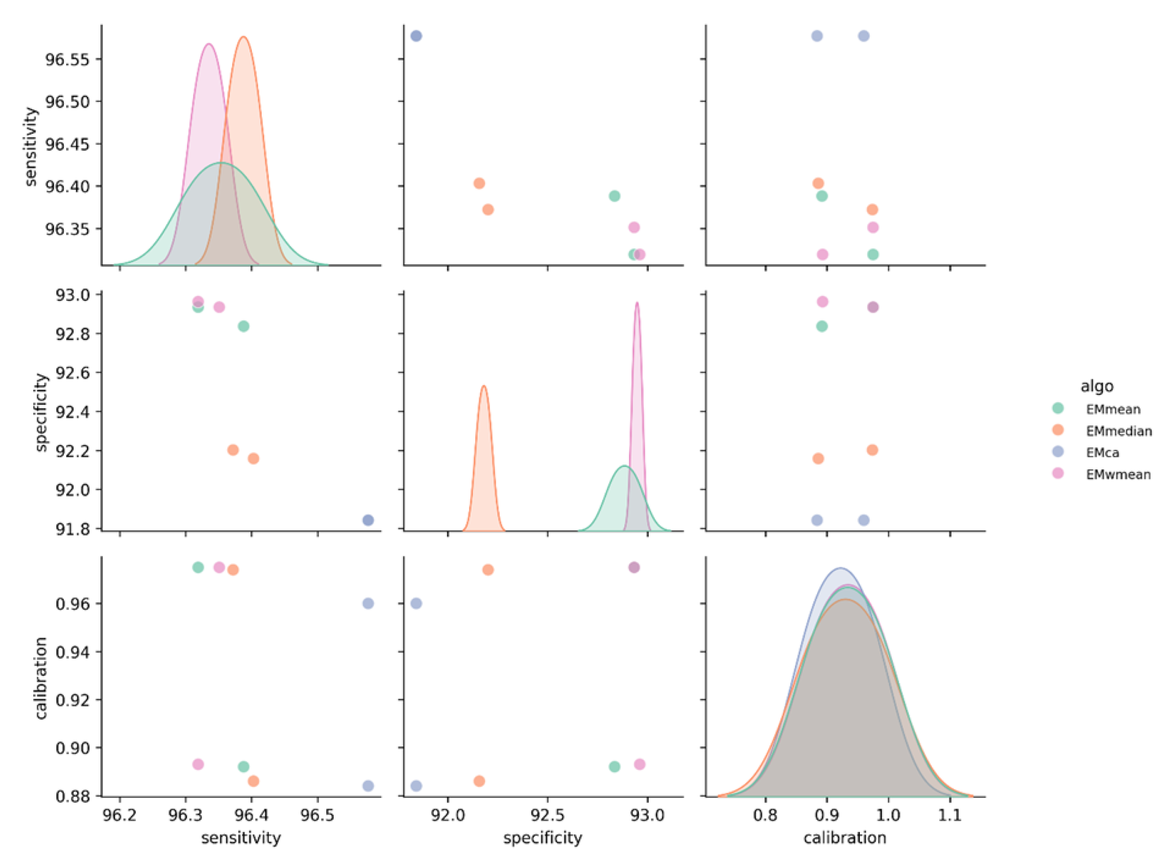
Based on eight single models, this study constructed and evaluated the performance of four ensemble models (EMmean, EMmedian, EMca, and EMwmean) (Figure 2). The results show that all ensemble models demonstrated excellent predictive accuracy (TSS > 0.88; AUC > 0.96). Among them, the weighted mean ensemble model (EMwmean) showed the best overall performance, with a TSS score of 0.893 and an AUC of 0.975, while maintaining high levels of sensitivity (96.3%) and specificity (93.0%). Based on this evaluation, EMwmean was ultimately selected as the core model for subsequent habitat predictions.

3.2. Environmental Factor Contributions

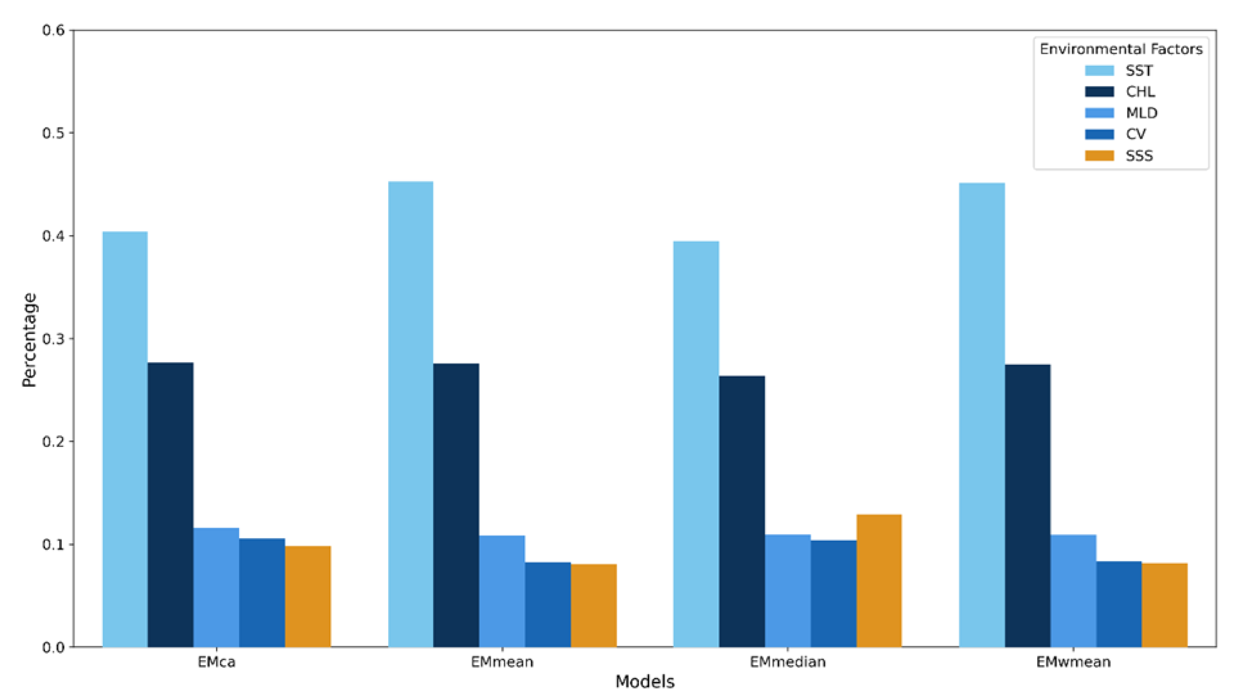
SST and CHL were identified as the decisive environmental factors shaping the species’ habitat patterns. This conclusion proved to be highly robust, holding true across all individual models (see Supplementary Materials, Figure S1) and ensemble models (Figure 3). In all models, the contribution rate of SST was by far the highest, ranging from 39.5% to 45.3%, making it the primary driver affecting the species’ distribution. As a key indicator of marine primary productivity, CHL was the second most important influencing factor, with its contribution rate stable at approximately 26% to 28%. The cumulative contribution of these two factors is extremely high, explaining over 65% of the variance in species distribution across all models. In comparison, the contributions of MLD, CV, and SSS were relatively small. The ranking of environmental factor importance (SST > CHL > MLD > SSS/CV) was completely consistent across all four ensemble methods.
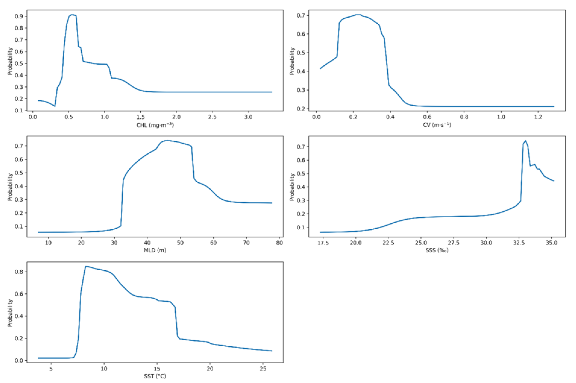
The response curves from the selected EMwmean model reveal the precise environmental thresholds that define the suitable ecological niche of Pacific saury (Figure 4). Habitat suitability peaked within a narrow SST range of 9–10 °C, declining rapidly in waters below 7 °C or above 15 °C. Suitability was highest at a CHL concentration of approximately 0.5 mg m−3. The species also showed a preference for a mixed layer depth (MLD) between 33 and 55 m, low current velocities (<0.3 m s−1), and Sea Surface Salinity (SSS) exceeding 32.5‰.

3.3. Habitat Distribution Prediction

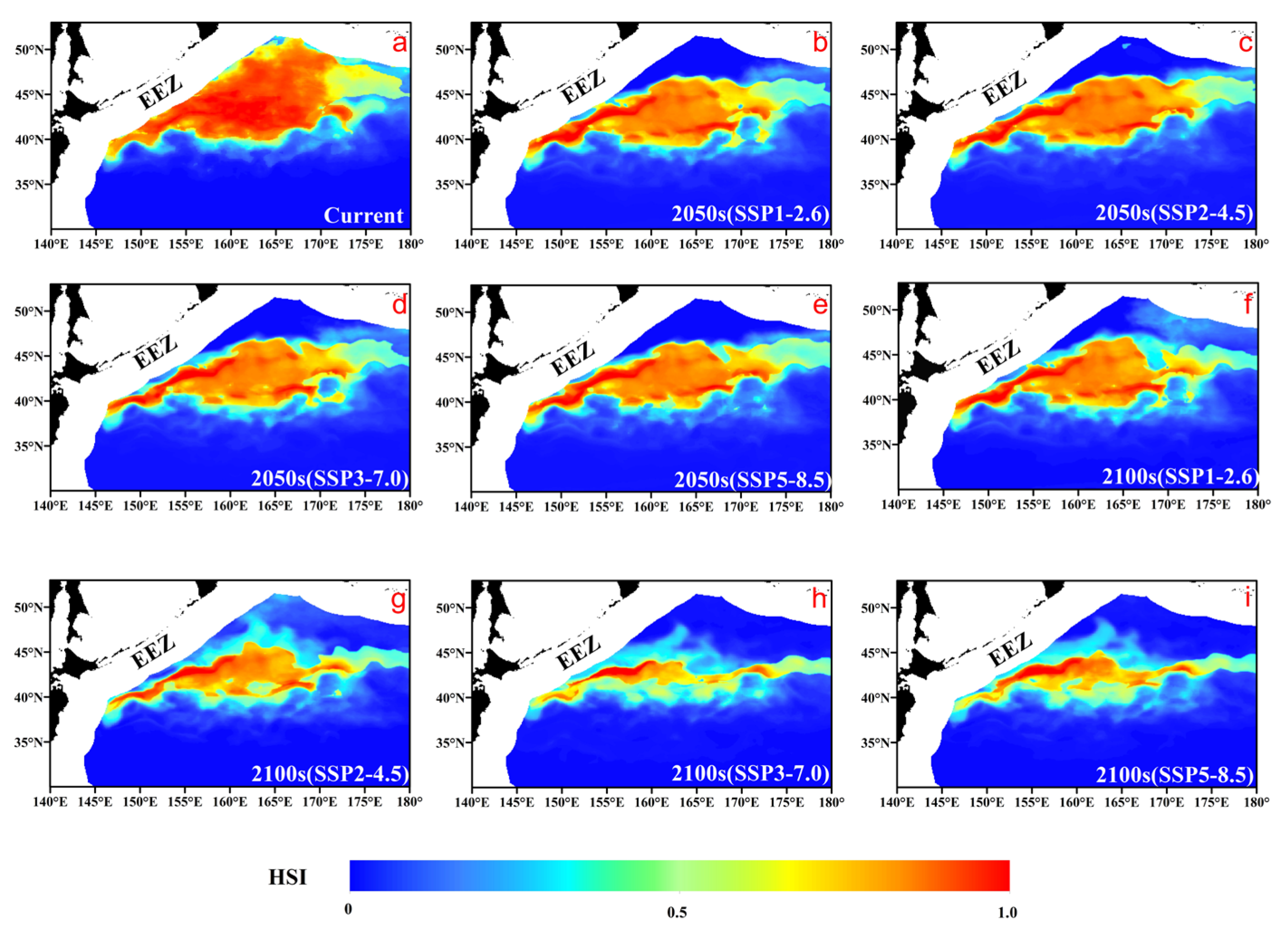
In terms of area (Figure 5 and Table 1), projections indicate a decline in both the quality and area of the species’ habitat, with the main trends being a reduction in highly suitable habitats, an expansion of unsuitable areas, and an overall distribution shift to the north and east. The decline in habitat quality is concentrated in the changes to the high-suitability areas (HSI 0.8–1.0). Under the high-emission scenario (SSP3-7.0), this highly suitable area is projected to decrease from the current 1.2 million km2 to just 67,000 km2 by the end of the century—a reduction of 94%, representing a substantial decrease in the availability of highly suitable habitat. Concurrently, the unsuitable area (HSI 0–0.4) is projected to expand by 12.1%, while the moderately suitable area (HSI 0.6–0.8), which acts as a buffer, will also decrease by nearly 40%.
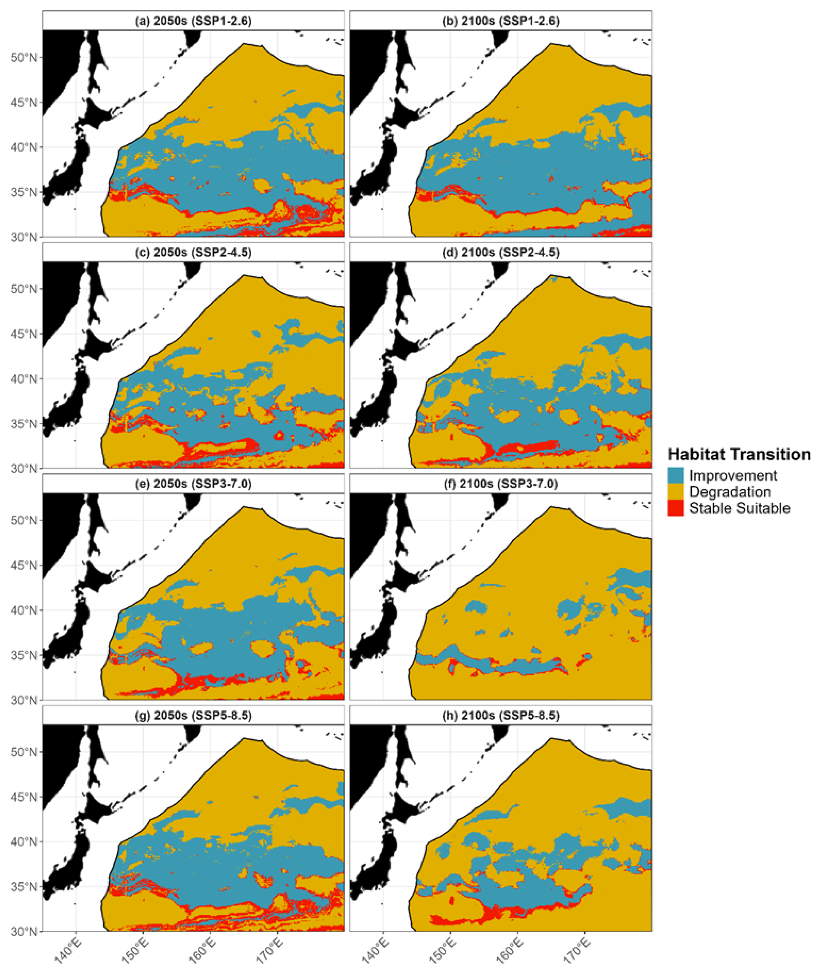
According to the simulations of future habitat transitions, three trends were observed: degradation, improvement, and stability, with their relative areas showing clear differences across different time periods and emission scenarios (Figure 6; see Supplementary Materials, Table S5, for detailed data). By mid-century (the 2050s), the areas of habitat degradation and improvement were relatively balanced. For example, under the low-emission SSP1-2.6 scenario, the area of improvement was approximately 2.32 million km2, comparable to the 2.82 million km2 degradation area. However, by the end of the century (the 2100s), the degradation trend became dominant. Under the high-emission SSP3-7.0 scenario, the degradation area expanded to 4.95 million km2, while the area available for improvement shrank to less than 0.6 million km2. The area of the “Stable Suitable” zone is projected to decrease from approximately 0.38 million km2 in the 2050s to about 0.11 million km2 in the 2100s under the high-emission SSP3-7.0 scenario.
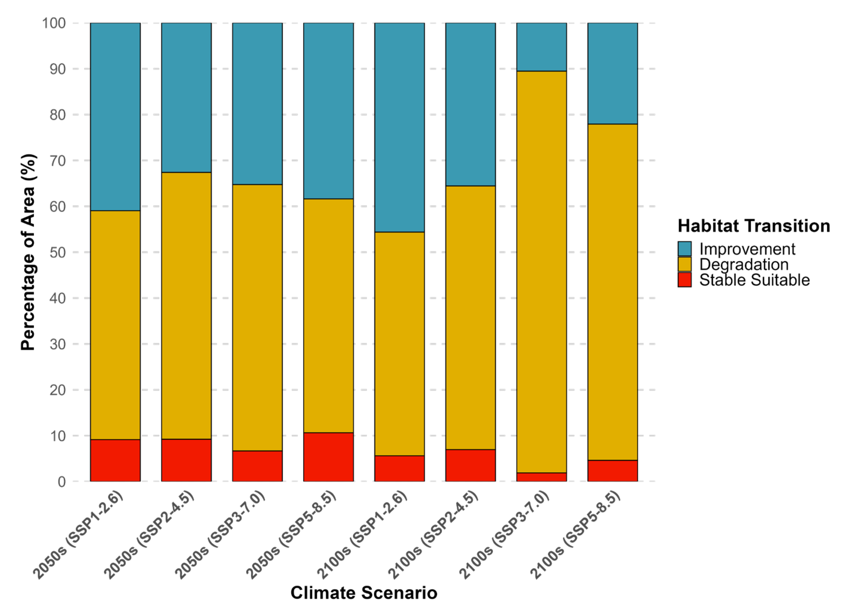
To provide a clearer, quantitative summary of these habitat transitions, the proportional changes in area were visualized in a stacked bar chart (Figure 7). This chart highlights the dominance of the “Degradation” trend, especially by the end of the century. Under the high-emission SSP3-7.0 scenario, habitat degradation is projected to account for 87.57% of the total area, while the stable suitable habitat shrinks to just 1.88%. In contrast, under the low-emission SSP1-2.6 scenario, the area of “Improvement” remains substantial (45.63%), and the “Degradation” area is much smaller (48.77%). The precise area (km2) and change rate (%) for all scenarios are detailed in the Supplementary Materials (Table S5).
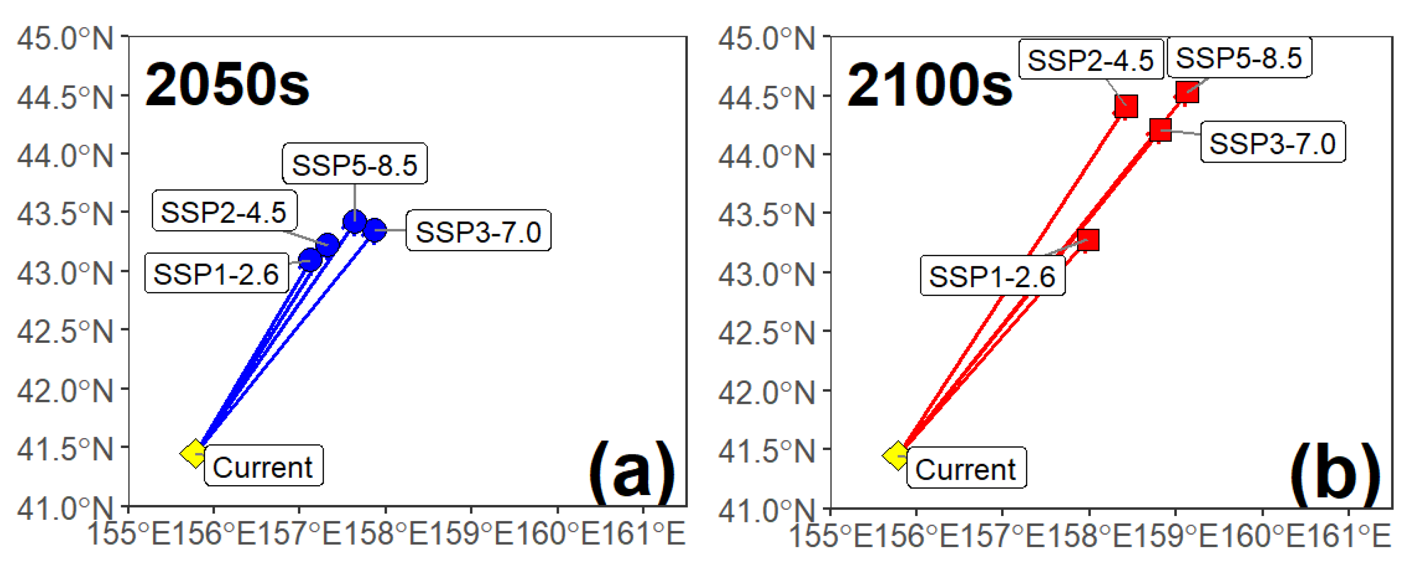
A consistent northeastward migration trend of the Pacific saury habitat centroid from its current position was observed under all future climate scenarios (Figure 8). By mid-century (the 2050s), the centroid shifted from its current position (approx. 155.8° E, 41.5° N) to a concentrated area between 157.1° E–157.9° E and 43.1° N–43.4° N. By the end of the century (the 2100s), this migration trend continues, but the displacement magnitudes and paths diverge significantly among the different emission scenarios. Under the high-emission scenarios SSP3-7.0 (approx. 158.8° E, 44.2° N) and SSP5-8.5 (approx. 159.1° E, 44.5° N), the centroid undergoes a much larger northeastward shift. In contrast, under the low-emission SSP1-2.6 scenario, the final position of the centroid (approx. 158.0°E, 43.3°N) was much closer to the 2050s cluster. The data indicate that while the overall direction is northeastward, the final migration distance is directly related to emission intensity, with high-emission scenarios leading to a farther displacement.

4. Discussion

4.1. Model Robustness and Interpretation of Ecological Drivers

Previous studies on Pacific saury habitats have relied on fishery logbooks, remote sensing, or scientific surveys [20,28], with few utilizing high-frequency vessel position data [11]. Our study employs Automatic Identification System (AIS) data from the Chinese distant-water fleet, processed via a deep learning model to extract fishing points for an ensemble species distribution model (ESDM). While single-nation data may miss some multi-national fishery dynamics, the Chinese fleet covers major high-seas fishing grounds, and our trends align with broader studies [7]. Unlike logbooks, which suffer from limited coverage and biases, AIS data offer dynamic, high-resolution insights into fishing responses to environmental changes, improving habitat hotspot identification, which strengthens spatial management applications such as the design of dynamic protected areas [29].
The ESDM achieved robust accuracy (TSS = 0.893, AUC = 0.975, sensitivity = 96.3%, specificity = 93.0%), validating its utility as a decision-support tool for fisheries management under uncertainty [21]. Sea surface temperature (SST) and chlorophyll-a (CHL) dominate habitat distribution (39.5–45.3% and 26–28% contribution, respectively), consistent with prior research [7,20]. This indicates Pacific saury’s distribution is highly sensitive to ocean temperature and primary productivity fluctuations, guiding monitoring priorities. SST regulates metabolism and water column structure [30], while CHL reflects zooplankton availability, with saury avoiding oligotrophic and eutrophic conditions [31]. Secondary factors—mixed layer depth (MLD), ocean current velocity (CV), and sea surface salinity (SSS)—support its preference for specific thermal, current, and high-salinity (>32.5‰) environments [27,28].
As a stenothermal pelagic fish, Pacific saury thrives in a narrow thermal window of 8–12 °C [19,20]; above this range, metabolic rate and reproductive success decline [32], a sensitivity that our model confirms with a sharp suitability drop outside these optimal temperatures. Climate-driven northward shifts in the 12 °C isotherm, especially in southern marginal seas (e.g., coastal Japan), reduce traditional habitat functionality, forcing migrations. The northeastward shift in the Kuroshio–Oyashio Transition Zone creates a new ‘ecological sweet spot’ with optimal temperatures and food availability [6]. Similar shifts in herring and cod suggest global warming is redefining marine species’ ecological boundaries [4,10,33].

4.2. Future Spatiotemporal Habitat Shifts and Their Ecological Implications

Climate change drives community-level shifts among small pelagic fish in the Northwest Pacific, including chub mackerel (Scomber japonicus) and Japanese sardine (Sardinops melanostictus) [23,33]. Understanding Pacific saury’s response is critical for ecosystem-based management. Our study addresses a research gap in systematic, quantitative forecasts of its habitat evolution under climate scenarios by combining high-resolution AIS data with an ensemble species distribution model (ESDM) [10]. While our model is based on the Chinese fleet, our findings on the species’ northeastward shift align with broader multi-national trends [7], providing robust insights into Pacific saury’s future within the pelagic community.
Projections show three trends: a drastic contraction of highly suitable habitat (HSI > 0.8), a northeastward centroid shift, and divergent outcomes across emission scenarios. Currently, 1.2 million km2 of highly suitable habitat supports population reproduction, but under SSP3-7.0, this shrinks to 67,000 km2 by 2100—a 94% reduction, signifying a substantial decrease in prime habitat. Unsuitable areas (HSI 0–0.4) expand by 12.1% (10.89 to 12.21 million km2), and stable suitable areas drop from 0.38 million km2 (2050s) to 0.11 million km2 (2100s), undermining habitat resilience. This continuous shrinkage of ecological refugia risks population viability, shifting habitats from a robust, contiguous core to a fragmented, lower-quality state. By 2050s, habitat improvement (2.32 million km2 under SSP1-2.6) and degradation (2.82 million km2) balance, but by 2100, degradation dominates (5 million km2 under SSP3-7.0), with improvement areas shrinking to <0.6 million km2, reflecting high-emission pathways’ inhibitory effect on ecosystem recovery. The habitat centroid shifts from 155.8° E, 41.5° N to 159.1° E, 44.5° N by 2100 under SSP5-8.5, a >400 km displacement driven by the Kuroshio-Oyashio Transition Zone’s northward shift and thermal stress in southern habitats [6]. Pacific saury, preferring specific temperatures and zooplankton concentrations, benefits from this ‘ecological sweet spot’ with suitable conditions [7]. However, paths diverge by century’s end, reflecting climate change’s cumulative effects, with SSP1-2.6 showing a smaller shift (158.0° E, 43.3° N). Yet, geographical migration may not ensure ecological success. High-latitude regions may lack sufficient zooplankton [8], and long-distance migration could strain reproductive success. A potential trophic mismatch may occur if saury’s rapid shift outpaces predators like tuna or seabirds, though further research is needed to confirm food web impacts [32]. Such disruptions challenge single-species management, risking regional fishery stability. For the North Pacific Fisheries Commission (NPFC), these findings inform adaptive strategies to address climate-driven shifts. The >400 km centroid shift under high-emission scenarios requires re-evaluating international quota allocations, as historical distributions become outdated. The 94% habitat contraction necessitates spatial planning to optimize fishing effort, prioritizing persistent suitable areas to reduce ecological impacts. Stable suitable zones, shrinking from 0.38 million km2 (2050s) to 0.11 million km2 (2100s), suggest potential climate refugia for conservation, such as protected areas to bolster population resilience. However, key caveats limit projections: (1) niche conservatism assumes static ecological preferences, potentially overlooking adaptation to warming oceans [33]; (2) single-nation AIS data, while robust for major fishing grounds, may miss multi-national fishery dynamics; (3) omission of interspecific interactions with species like sardines and chub mackerel, whose overlapping habitats affect resource competition; and (4) uncertainties in Bio-Oracle’s downscaled climate data, particularly for small-scale oceanographic features [23,34].
While our model uses fishing locations as a proxy for species presence, it does not explicitly incorporate fishing effort as a variable. This is a common practice in large-scale habitat modeling where standardized effort data is unavailable. We acknowledge that changes in fishing technology, strategy, or intensity over time could influence the observed distribution of fishing activities. However, by using a highly standardized fleet (stick-held dip net) and a relatively short time frame for the baseline period (2019–2024), we have minimized the potential impact of such variations. Future work could benefit from integrating fine-scale effort data to further refine these projections.
Future research should prioritize mechanistic models (e.g., Individual-Based Models or Dynamic Energy Budget models) to link environmental changes [35,36], like rising SST, to population dynamics (growth, reproduction, survival). Multi-species distribution models (MSDMs) can address competitive interactions among pelagic fish [37,38,39], enhancing ecosystem-based management. Genomics and environmental DNA (eDNA) techniques should assess adaptive potential to new thermal or prey environments [40], improving model accuracy and management adaptability.

5. Conclusions

This study developed an innovative framework using high-resolution AIS data, deep learning, and ensemble models to predict Pacific saury habitat dynamics under climate change. Our model identified sea surface temperature (SST) and chlorophyll-a (CHL) as the core drivers shaping the species’ habitat. Projections reveal two severe threats under high-emission scenarios: a contraction of over 94% in highly suitable habitat and a northeastward migration of its centroid exceeding 400 km. This quantitative risk assessment signals profound challenges to the species’ viability and broader ecosystem stability, including potential “trophic mismatch”.
While these projections provide a critical foresight tool, they should be interpreted with caution given the methodological limitations outlined in the discussion, such as the assumption of niche conservatism and the use of single-nation fleet data. Ultimately, our work delivers an operational, science-based tool to support fisheries management bodies like the NPFC. By providing a quantitative risk assessment across different emission scenarios, these projections can directly inform the development of adaptive management strategies, including adjustments to international quota allocations, forward-looking spatial planning for fishing effort, and the identification of potential climate refugia for the species.

Supplementary Materials

The following supporting information can be downloaded at https://www.mdpi.com/article/10.3390/ani15192828/s1, Section S1: Detailed Description of the CNN-LSTM Model; Figure S1: Percentage contribution of environmental factors in the eight individual species distribution models; Table S1: Final Hyperparameters for the CNN-LSTM Model; Table S2: Final Model Performance Evaluation Report; Table S3: Environmental variables used in the species distribution models (SDMs) and their sources; Table S4: Summary of Single Model Performance Evaluation; Table S5: Area (km2) and change rate (%) of habitat transitions for Pacific saury under future climate scenarios.

Author Contributions

Conceptualization, H.Z. (Hanji Zhu), Y.L. and J.W.; methodology, H.Z. (Hanji Zhu) and S.H.; software, Y.S.; validation, Y.S.; resources, H.Z. (Heng Zhang); data curation, M.G. and F.Z.; writing—original draft preparation, H.Z. (Hanji Zhu), Y.L. and D.X.; writing—review and editing, H.Z. (Hanji Zhu), D.X. and J.W.; visualization, Y.S.; supervision, H.Z. (Heng Zhang) and L.L.; funding acquisition, H.Z. (Heng Zhang) and L.L. All authors have read and agreed to the published version of the manuscript.

Funding

This work was supported by the Program on the Survey of Pelagic Fishery Resources, sponsored by the Ministry of Agriculture and Rural Affairs; the Program on the Survey, Monitoring and Assessment of Global Fishery Resources (Comprehensive scientific survey of fisheries resources at the high seas), sponsored by the Ministry of Agriculture and Rural Affairs; the National Key Research and Development Project of China (2024YFD2400601); and the Zhejiang ocean fishery resources exploration and capture project (CTZB-2022080076).

Institutional Review Board Statement

The data used in this study include commercial fishing operation records, vessel positioning data, and marine environmental data. As no animal experiments were involved, approval from the local ethics committee is not required.

Informed Consent Statement

Not applicable.

Data Availability Statement

Environmental data are publicly available from the Copernicus Marine Environment Monitoring Service (CMEMS) and the Bio-Oracle v.3.0 database. R and Python scripts used for this study, along with a sample dataset, are available on GitHub: https://github.com/saury-habitat-study/Saury-Habitat-ESDM (accessed on 24 September 2025). The raw AIS vessel position dataset is not publicly available due to data sensitivity but may be obtained from the corresponding author upon reasonable request.

Acknowledgments

We would like to acknowledge Heng Zhang for his valuable guidance throughout this research, and we extend our gratitude to all authors for their contributions and support.

Conflicts of Interest

The authors declare no conflicts of interest.

References

  1. Cavole, L.M.; Demko, A.M.; Diner, R.E.; Giddings, A.; Koester, I.; Pagniello, C.M.; Paulsen, M.-L.; Ramirez-Valdez, A.; Schwenck, S.M.; Yen, N.K. Biological impacts of the 2013–2015 warm-water anomaly in the Northeast Pacific: Winners, losers, and the future. Oceanography 2016, 29, 273–285. [Google Scholar] [CrossRef]
  2. Gomes, D.G.; Ruzicka, J.J.; Crozier, L.G.; Huff, D.D.; Brodeur, R.D.; Stewart, J.D. Marine heatwaves disrupt ecosystem structure and function via altered food webs and energy flux. Nat. Commun. 2024, 15, 1988. [Google Scholar] [CrossRef]
  3. Barkhordarian, A.; Nielsen, D.M.; Baehr, J. Recent marine heatwaves in the North Pacific warming pool can be attributed to rising atmospheric levels of greenhouse gases. Commun. Earth Environ. 2022, 3, 131. [Google Scholar] [CrossRef]
  4. Buonanduci, M.S.; Buhle, E.R.; Case, M.J.; Howe, E.R.; Robertson, J.C.; Vanbuskirk, N.; Ettinger, A.K. Forest restoration can bolster salmon population persistence under climate change. Biol. Conserv. 2025, 305, 111099. [Google Scholar] [CrossRef]
  5. Pinsky, M.L.; Worm, B.; Fogarty, M.J.; Sarmiento, J.L.; Levin, S.A. Marine taxa track local climate velocities. Science 2013, 341, 1239–1242. [Google Scholar] [CrossRef] [PubMed]
  6. Shen, J.; Han, S.; Fan, W. Saury resource and fishing grounds in the Northwest Pacific. Mar. Fish. 2004, 1, 61–65. [Google Scholar] [CrossRef]
  7. Chang, Y.J.; Lan, K.W.; Walsh, W.A.; Hsu, J.; Hsieh, C.H. Modelling the impacts of environmental variation on habitat suitability for Pacific saury in the Northwestern Pacific Ocean. Fish. Oceanogr. 2019, 28, 291–304. [Google Scholar] [CrossRef]
  8. Hua, C.; Zhu, Q.; Xu, W.; Song, L. Review of the life history, resources and fishing grounds of the Pacific saury in the North Pacific Ocean. J. Fish. Sci. China 2019, 26, 811–821. [Google Scholar]
  9. Xiang, D.; Sun, Y.; Zhu, H.; Wang, J.; Huang, S.; Zhang, S.; Zhang, F.; Zhang, H. Comparative Analysis of Prediction Models for Trawling Grounds of the Argentine Shortfin Squid Illex argentinus in the Southwest Atlantic High Seas Based on Vessel Position and Fishing Log Data. Biology 2025, 14, 35. [Google Scholar] [CrossRef]
  10. Zhang, H.; Sun, Y.; Zhu, H.; Xiang, D.; Wang, J.; Zhang, F.; Huang, S.; Li, Y. Simulation and Identification of the Habitat of Antarctic Krill Based on Vessel Position Data and Integrated Species Distribution Model: A Case Study of Pumping-Suction Beam Trawl Fishing Vessels. Animals 2025, 15, 1557. [Google Scholar] [CrossRef]
  11. Xue, M.; Tong, J.; Ma, W.; Zhu, Z.; Wang, W.; Lyu, S.; Chen, X. Reimagining habitat suitability modeling for Pacific saury (Cololabis saira) in the Northwest Pacific Ocean through acoustic data analysis from fishing vessels. Ecol. Inform. 2025, 85, 102971. [Google Scholar] [CrossRef]
  12. Yang, T.; Liu, X.; Han, Z. Predicting the effects of climate change on the suitable habitat of Japanese Spanish mackerel (Scomberomorus niphonius) based on the species distribution model. Front. Mar. Sci. 2022, 9, 927790. [Google Scholar] [CrossRef]
  13. Zhang, J.; Li, J.; Cai, Y.; Zhang, K.; Xu, Y.; Chen, Z.; Xu, S. Simulating Habitat Suitability Changes of Threadfin Porgy (Evynnis cardinalis) in the Northern South China Sea Using Ensemble Models Under Medium-to-Long-Term Future Climate Scenarios. Biology 2025, 14, 236. [Google Scholar] [CrossRef] [PubMed]
  14. Shepperson, J.L.; Hintzen, N.T.; Szostek, C.L.; Bell, E.; Murray, L.G.; Kaiser, M.J. A comparison of VMS and AIS data: The effect of data coverage and vessel position recording frequency on estimates of fishing footprints. ICES J. Mar. Sci. 2018, 75, 988–998. [Google Scholar] [CrossRef]
  15. Katara, I.; Silva, A. Mismatch between VMS data temporal resolution and fishing activity time scales. Fish. Res. 2017, 188, 1–5. [Google Scholar] [CrossRef]
  16. Thuiller, W.; Lafourcade, B.; Engler, R.; Araújo, M.B. BIOMOD—A platform for ensemble forecasting of species distributions. Ecography 2009, 32, 369–373. [Google Scholar] [CrossRef]
  17. Warren, D.L.; Glor, R.E.; Turelli, M. ENMTools: A toolbox for comparative studies of environmental niche models. Ecography 2010, 33, 607–611. [Google Scholar] [CrossRef]
  18. Huang, W.-B.; Lo, N.C.; Chiu, T.-S.; Chen, C.-S. Geographical distribution and abundance of Pacific saury, Cololabis saira (Brevoort)(Scomberesocidae), fishing stocks in the Northwestern Pacific in relation to sea temperatures. Zool. Stud. 2007, 46, 705. [Google Scholar]
  19. Tian, Y.; Akamine, T.; Suda, M. Variations in the abundance of Pacific saury (Cololabis saira) from the northwestern Pacific in relation to oceanic-climate changes. Fish. Res. 2003, 60, 439–454. [Google Scholar] [CrossRef]
  20. Tseng, C.-T.; Su, N.-J.; Sun, C.-L.; Punt, A.E.; Yeh, S.-Z.; Liu, D.-C.; Su, W.-C. Spatial and temporal variability of the Pacific saury (Cololabis saira) distribution in the northwestern Pacific Ocean. ICES J. Mar. Sci. 2013, 70, 991–999. [Google Scholar] [CrossRef]
  21. Sun, Y.; Zhang, H.; Jiang, K.; Xiang, D.; Shi, Y.; Huang, S.; Li, Y.; Han, H. Simulating the changes of the habitats suitability of chub mackerel (Scomber japonicus) in the high seas of the North Pacific Ocean using ensemble models under medium to long-term future climate scenarios. Mar. Pollut. Bull. 2024, 207, 116873. [Google Scholar] [CrossRef] [PubMed]
  22. Dormann, C.F.; Elith, J.; Bacher, S.; Buchmann, C.; Carl, G.; Carré, G.; Marquéz, J.R.G.; Gruber, B.; Lafourcade, B.; Leitão, P.J. Collinearity: A review of methods to deal with it and a simulation study evaluating their performance. Ecography 2013, 36, 27–46. [Google Scholar] [CrossRef]
  23. Sun, Y.; Xiang, D.; Wang, J.; Jiang, K.; Zhu, H.; Huang, S.; Zhang, F.; Li, Y.; Zhang, H. Comparative analysis of modeling methods and prediction accuracy for Japanese sardine habitat under three climate scenarios with differing greenhouse emission pathways. Mar. Pollut. Bull. 2025, 215, 117867. [Google Scholar] [CrossRef] [PubMed]
  24. Wisz, M.S.; Hijmans, R.; Li, J.; Peterson, A.T.; Graham, C.; Guisan, A.; Group, N.P.S.D.W. Effects of sample size on the performance of species distribution models. Divers. Distrib. 2008, 14, 763–773. [Google Scholar] [CrossRef]
  25. Allouche, O.; Tsoar, A.; Kadmon, R. Assessing the accuracy of species distribution models: Prevalence, kappa and the true skill statistic (TSS). J. Appl. Ecol. 2006, 43, 1223–1232. [Google Scholar] [CrossRef]
  26. Araújo, M.B.; New, M. Ensemble forecasting of species distributions. Trends Ecol. Evol. 2007, 22, 42–47. [Google Scholar] [CrossRef]
  27. Davies, S.C.; Thompson, P.L.; Gomez, C.; Nephin, J.; Knudby, A.; Park, A.E.; Friesen, S.K.; Pollock, L.J.; Rubidge, E.M.; Anderson, S.C. Addressing uncertainty when projecting marine species’ distributions under climate change. Ecography 2023, 2023, e06731. [Google Scholar] [CrossRef]
  28. Hua, C.; Li, F.; Zhu, Q.; Zhu, G.; Meng, L. Habitat suitability of Pacific saury (Cololabis saira) based on a yield-density model and weighted analysis. Fish. Res. 2020, 221, 105408. [Google Scholar] [CrossRef]
  29. Karp, M.A.; Brodie, S.; Smith, J.A.; Richerson, K.; Selden, R.L.; Liu, O.R.; Muhling, B.A.; Samhouri, J.F.; Barnett, L.A.; Hazen, E.L. Projecting species distributions using fishery-dependent data. Fish Fish. 2023, 24, 71–92. [Google Scholar] [CrossRef]
  30. Pörtner, H.O.; Farrell, A.P. Physiology and climate change. Science 2008, 322, 690–692. [Google Scholar] [CrossRef]
  31. Chassot, E.; Bonhommeau, S.; Dulvy, N.K.; Mélin, F.; Watson, R.; Gascuel, D.; Le Pape, O. Global marine primary production constrains fisheries catches. Ecol. Lett. 2010, 13, 495–505. [Google Scholar] [CrossRef]
  32. Pörtner, H.O.; Knust, R. Climate Change Affects Marine Fishes Through the Oxygen Limitation of Thermal Tolerance. Science 2007, 315, 95–97. [Google Scholar] [CrossRef]
  33. Liu, S.; Zhang, H.; Yang, C.; Fang, Z. Differences in habitat distribution of Sardinops melanostictus and Scomber japonicus in the northwest Pacific based on a maximum entropy model. J. Shanghai Ocean Univ. 2023, 32, 806–817. [Google Scholar] [CrossRef]
  34. Edwards, M.; Richardson, A.J. Impact of climate change on marine pelagic phenology and trophic mismatch. Nature 2004, 430, 881–884. [Google Scholar] [CrossRef]
  35. Pecquerie, L.; Petitgas, P.; Kooijman, S.A. Modeling fish growth and reproduction in the context of the Dynamic Energy Budget theory to predict environmental impact on anchovy spawning duration. J. Sea Res. 2009, 62, 93–105. [Google Scholar] [CrossRef]
  36. Nisbet, R.M.; Jusup, M.; Klanjscek, T.; Pecquerie, L. Integrating dynamic energy budget (DEB) theory with traditional bioenergetic models. J. Exp. Biol. 2012, 215, 892–902. [Google Scholar] [CrossRef] [PubMed]
  37. Erickson, K.D.; Smith, A.B. Modeling the rarest of the rare: A comparison between multi-species distribution models, ensembles of small models, and single-species models at extremely low sample sizes. Ecography 2023, 2023, e06500. [Google Scholar] [CrossRef]
  38. Panzeri, D.; Russo, T.; Arneri, E.; Carlucci, R.; Cossarini, G.; Isajlović, I.; Krstulović Šifner, S.; Manfredi, C.; Masnadi, F.; Reale, M. Identifying priority areas for spatial management of mixed fisheries using ensemble of multi-species distribution models. Fish Fish. 2024, 25, 187–204. [Google Scholar] [CrossRef]
  39. McMillan, M.N.; Leahy, S.M.; Hillcoat, K.B.; Wickens, M.; Roberts, E.M.; Daniell, J.J. Untangling multi-species fisheries data with species distribution models. Rev. Fish Biol. Fish. 2024, 34, 1133–1148. [Google Scholar] [CrossRef]
  40. Rourke, M.L.; Fowler, A.M.; Hughes, J.M.; Broadhurst, M.K.; DiBattista, J.D.; Fielder, S.; Wilkes Walburn, J.; Furlan, E.M. Environmental DNA (eDNA) as a tool for assessing fish biomass: A review of approaches and future considerations for resource surveys. Environ. DNA 2022, 4, 9–33. [Google Scholar] [CrossRef]
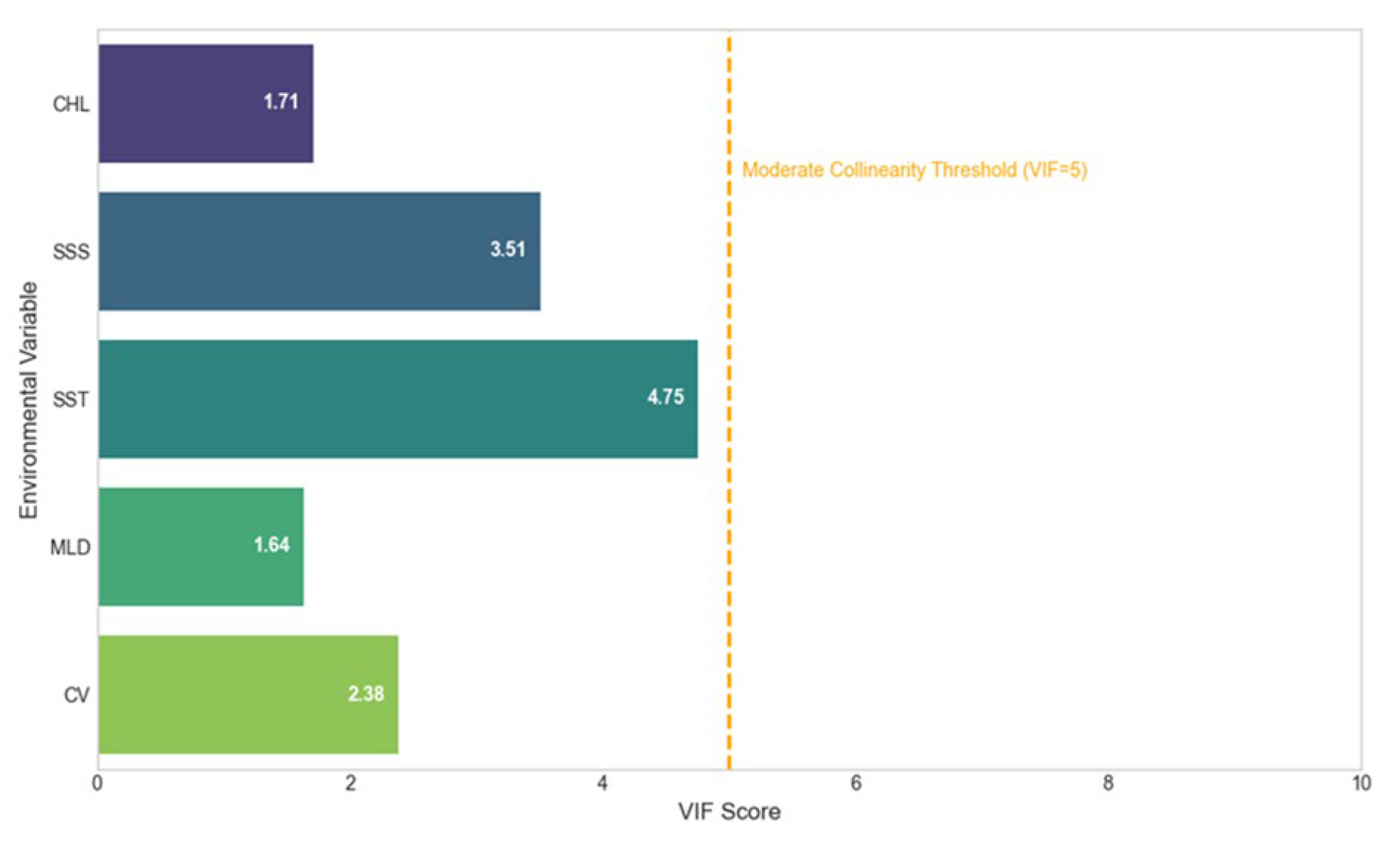
Figure 1. VIF Collinearity Diagnostics for Environmental Factors. The dashed orange line indicates the moderate collinearity threshold (VIF = 5).
Animals 15 02828 g001
Figure 2. Comparative analysis among the four ensemble models.
Animals 15 02828 g002
Figure 3. Percentage contribution of environmental factors in the ensemble models.
Animals 15 02828 g003
Figure 4. Response curves of habitat suitability for each environmental factor under the ensemble weighted model.
Animals 15 02828 g004
Figure 5. Projected changes in Pacific saury habitat suitability (HSI) for (a) the current period; the 2050s under scenarios (b) SSP1-2.6, (c) SSP2-4.5, (d) SSP3-7.0, and (e) SSP5-8.5; and the 2100s under scenarios (f) SSP1-2.6, (g) SSP2-4.5, (h) SSP3-7.0, and (i) SSP5-8.5.
Animals 15 02828 g005
Figure 6. Habitat transition maps for Pacific saury under four future climate scenarios. The subfigures show transitions for the (a) 2050s and (b) 2100s under SSP1-2.6; (c) 2050s and (d) 2100s under SSP2-4.5; (e) 2050s and (f) 2100s under SSP3-7.0; and (g) 2050s and (h) 2100s under SSP5-8.5. Blue, orange, and red areas represent zones of habitat improvement, degradation, and stability, respectively, relative to the current distribution.
Animals 15 02828 g006
Figure 7. Proportional changes in Pacific saury habitat under future climate scenarios. The stacked bar chart shows the percentage of the current suitable habitat area projected to undergo Improvement (blue), Degradation (orange), or remain Stable Suitable (red) for each time period and Shared Socioeconomic Pathway (SSP).
Animals 15 02828 g007
Figure 8. Centroid shift in Pacific saury habitat under different future climate scenarios. (a) Projected shift from the current period to the 2050s; (b) Projected shift from the current period to the 2100s.
Animals 15 02828 g008
Table 1. Changes in the area of Pacific saury habitat on the high seas in different suitability zones.
Period and
Climate Scenarios
Habitat Suitability Index (HSI) Range
Non-Suitable
Areas (0–0.4) (km2)
Low Suitable
Area (0.4–0.6) (km2)
Moderately Suitable
Area (0.6–0.8) (km2)
Highly Suitable
Area (0.8–1.0) (km2)
Current10,894,427471,397360,9391,200,282
2050s SSP1-2.611,386,961345,528465,098719,241
2050s SSP2-4.511,432,190343,446375,633765,558
2050s SSP3-7.011,528,263343,727467,651577,186
2050s SSP5-8.511,500,569376,849366,425672,985
2100s SSP1-2.611,566,635337,221388,768624,203
2100s SSP2-4.511,847,665412,899371,439284,824
2100s SSP3-7.012,213,550417,520218,89366,865
2100s SSP5-8.511,927,266538,183265,671185,707
Disclaimer/Publisher’s Note: The statements, opinions and data contained in all publications are solely those of the individual author(s) and contributor(s) and not of MDPI and/or the editor(s). MDPI and/or the editor(s) disclaim responsibility for any injury to people or property resulting from any ideas, methods, instructions or products referred to in the content.