1. Introduction
Current commercial accelerometers are classified as piezoelectric, capacitive and piezoresistive. Thermal convection-based accelerometers are promising, but some requirements still need to be met [
1]. Capacitive accelerometers are the most common currently used, with superior performance at low frequencies. They have several advantages, like having high sensitivity, simple transduction, readout circuitry, low noise level, less immunity to temperature linearity, a lower area, low power consumption, stable direct current characteristics [
2], amenability for feedback [
3] and compatibility with MEMS and Complementary Metal Oxide Semiconductor (CMOS) fabrication processes [
4]. They typically consist of four components: a moving mass, called proof or seismic mass; a suspension formed by one or more elastic supports and springs; a shock absorber; and a mechanism by which displacement of the moving mass is recorded. Acceleration forces may be static, like the constant force of gravity (g force), or dynamic, caused by moving or vibrating the accelerometer [
5].
To improve the mechanical sensitivity of accelerometers, one of the main strategies focused on the shapes of the beams. Several cantilevers’ beams, which are the base of the accelerometer springs, have been reported, and some of them are presented in
Table 1. In [
6], rectangular, stepped rectangular cantilevers and optimized stepped cantilevers are given. The largest sensitivity corresponds to the optimized geometry. Sensitivity values are normalized with reference to the characteristics of the normal rectangular cantilever (1, 2.82 and 3.16, respectively). The reaction force is not provided for any cantilever, while stress and natural frequency are not given for all cases.
Table 2 shows capacitive accelerometers with different beam geometries. The importance of the selection of the beam is also noted, which represents the suspension of the acceleration system. The reaction force of the structures is not considered among the provided parameters, and stress on beams is only considered in one of these cases. The authors of [
11,
12] provide voltage sensitivities of 0.24 and 3.16 V/g, respectively. Capacitive sensitivity is reported by [
13,
14] of 3.3 pF/G and 15.5 fF/g, respectively. Finally, mechanical sensitivity is given by [
14,
15] of 0.574 μm/g and 29.8 nm/g, respectively. The last sensitivity is of special interest for us because it provides information regarding the displacement capability of the structure when acceleration is applied.
In general, the design of beams is extremely important, including their shape, dimensions and materials, as they are determinants of the static and dynamic accelerometer response. Boundary conditions are also determinant in the results. The variation on beam geometries, or generating new shapes, represents an opportunity to increase the mechanical sensitivity of accelerometers, without a notable variation in their area.
The main challenge in this paper is to propose a novel geometry of arm, specifically focused on the increase in displacement. Consequently, a reduction in natural frequency will be also obtained, making it necessary to, additionally, look for a strategy to obtain a lower reduction of the natural frequency in accordance with the width of segments. The stress distribution on the beam and its impact on the proof mass are found also illustrative in determining the performance of the proposed new beam’s geometry.
The second challenge is to understand the velocity supported by the proposed beams, especially when a simulation of the accelerometer’s performance in a nonideal environment is considered with a damping factor different to zero.
In summary, this paper focuses on the design of a modified beam based on alternate segments, looking for a lower spring constant. The content of this work is organized as follows. In
Section 2, some basic concepts of accelerometers and their operation are presented.
Section 3 shows the designs of the implemented suspension beams and the results obtained. In
Section 4, harmonic response and explicit dynamic analyses are developed. In the same section, a comparison of the arm’s shape here proposed, with other accelerometers is shown. A variation in the width of the thinner segment is also performed. Finally, in
Section 5, some concluding remarks are given.
2. Capacitive Accelerometers
2.1. Some Basic Concepts
Accelerometers are based on Newton’s second law of motion:
where
p is the impulse momentum of a mass
m,
F is the force acting on the mass and
a is acceleration. The mass displacement is a measure for acceleration the mass is undergoing [
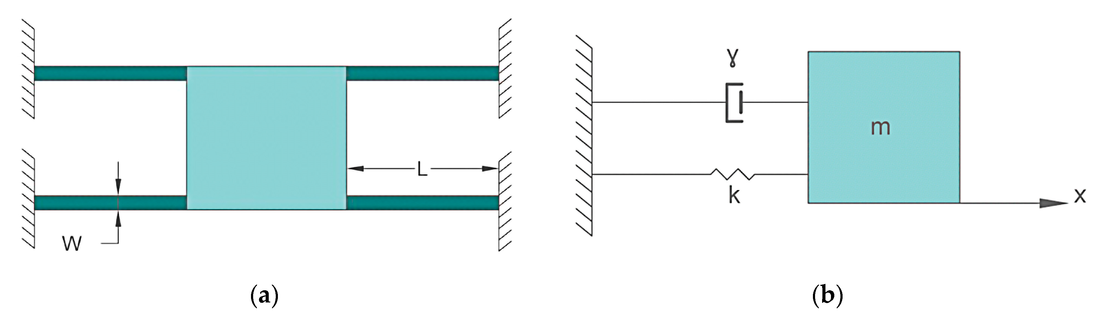
21]. The basic mechanical lumped model or damped mass–spring system model of a capacitive accelerometer is shown in
Figure 1. The proof (or seismic) mass
m is suspended by a flexible spring, with stiffness or spring constant
k. The vibrations are damped by introducing a fluid inside the package. The damping is represented by γ. Due to the inertia of the proof mass, the displacement
x can be used to measure the acceleration. Acceleration is measured by the displacement of the proof or seismic mass. The acceleration unit is g (9.81 m/s
2). A differential equation governing the motion is given by [
22]:
Equation (2) is the one-degree of freedom damped resonator equation, with a solution for the case
FE = 0, is given by Equation (3), which was obtained by the use of Laplace transformations, and considering the quality factor given by
, where
is the mechanical resonant frequency [
15,
22].
where
F is the external force acting on the mass. In general,
m = ρV, where
ρ is the material density and
V is the corresponding volume of mass, γ is the damping coefficient and
k is the spring constant.
2.2. Static Performance
The static deflection of the microcantilevers is related to the difference in surface stress of the two faces of the microcantilever caused by an external force or load or stress generated on or within the cantilever. Under static conditions, such as constant acceleration applied, at frequencies below the resonant frequency (ω << ω
0), the behavior of the accelerometer is determined by the proof mass and the stiffness of the suspension beam [
21]:
where
x is the proof mass displacement,
a is the applied acceleration value,
m is the mass and
k is the spring constant. Resonance frequency is also obtained from displacement equation,
.
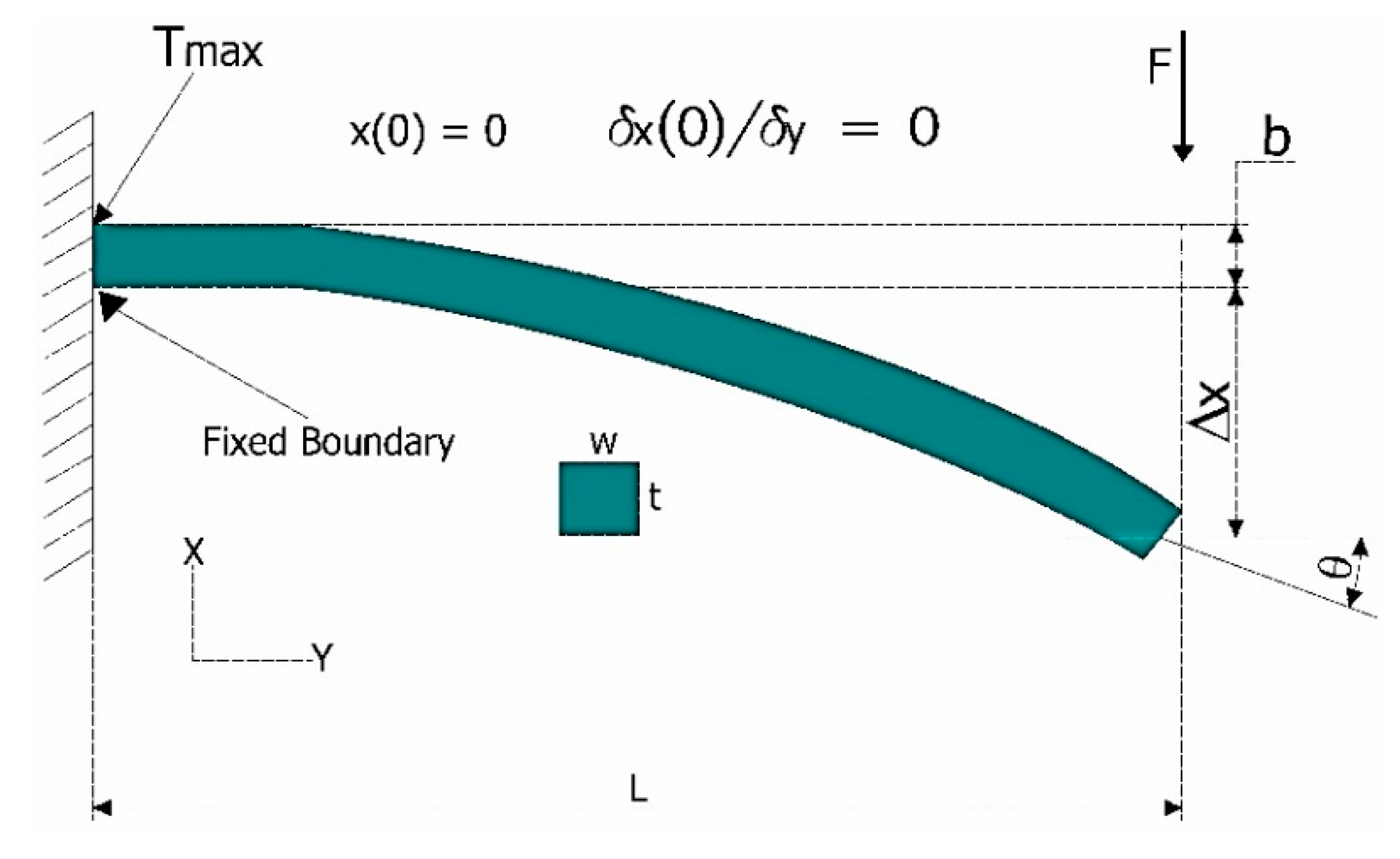
The spring constant for the case of a uniform geometry is calculated from the analysis of the uniform a cantilever of length
L, width
w and thickness
t, shown in
Figure 2.
The applied force
F, and the boundary conditions, produce the cantilever bending, which is governed by the moment–curvature relationship [
22,
23],
, where
x(y) is the displacement.
E is Young’s modulus of elasticity and
I =
wt3/12 is the second moment of inertia. The boundary conditions are
x (0) = 0 and
. From the moment–curvature relationship, the beam displacement, or the equation of the elastic curve, is obtained:
The effective stiffness constant is given by the comparison of the simplified equation of the elastic curve
and Hooke’s Law, by:
The normal or flexural stress in the beam is obtained from strain
ε(
x,
y) considering pure bending, and
R as the curvature radio. The maximum value of bending stress is located at
y = 0, on the beam surfaces (
x = ±
t/2):
3. Design and Simulation of Devices
To compare the accelerometer’s performance, the total proof mass and total lengths of beams are kept constant, with conventional uniform springs and retaining the proposed modified shape. For the alternate segment’s distribution of symmetric beams, the width of the uniform beam is taken as reference. The design ideas were as follows: the presence of a thin flexure at the anchor to generate a larger movement and a sequence of segments of different masses to reduce the stiffness, as a consequence of the mass reduction on the beam.
The performance analysis of the uniform and proposed beams was performed considering three cases: ¼, ½ and complete accelerometer. The ¼ accelerometer is composed of one beam and ¼ of the proof mass. The ½ accelerometer is composed of two beams and half of the proof mass. The complete accelerometer, as usual, is composed of four suspension beams and a complete proof mass. In each case, to calculate the displacement of an accelerometer with a symmetrical geometry shape of beams, mathematical relationships, based on Equation (5), were developed. For the case of force and stress, the simplified equation of the elastic curve and equation of maximum value of bending stress (Equation (7)) were also considered and adjusted.
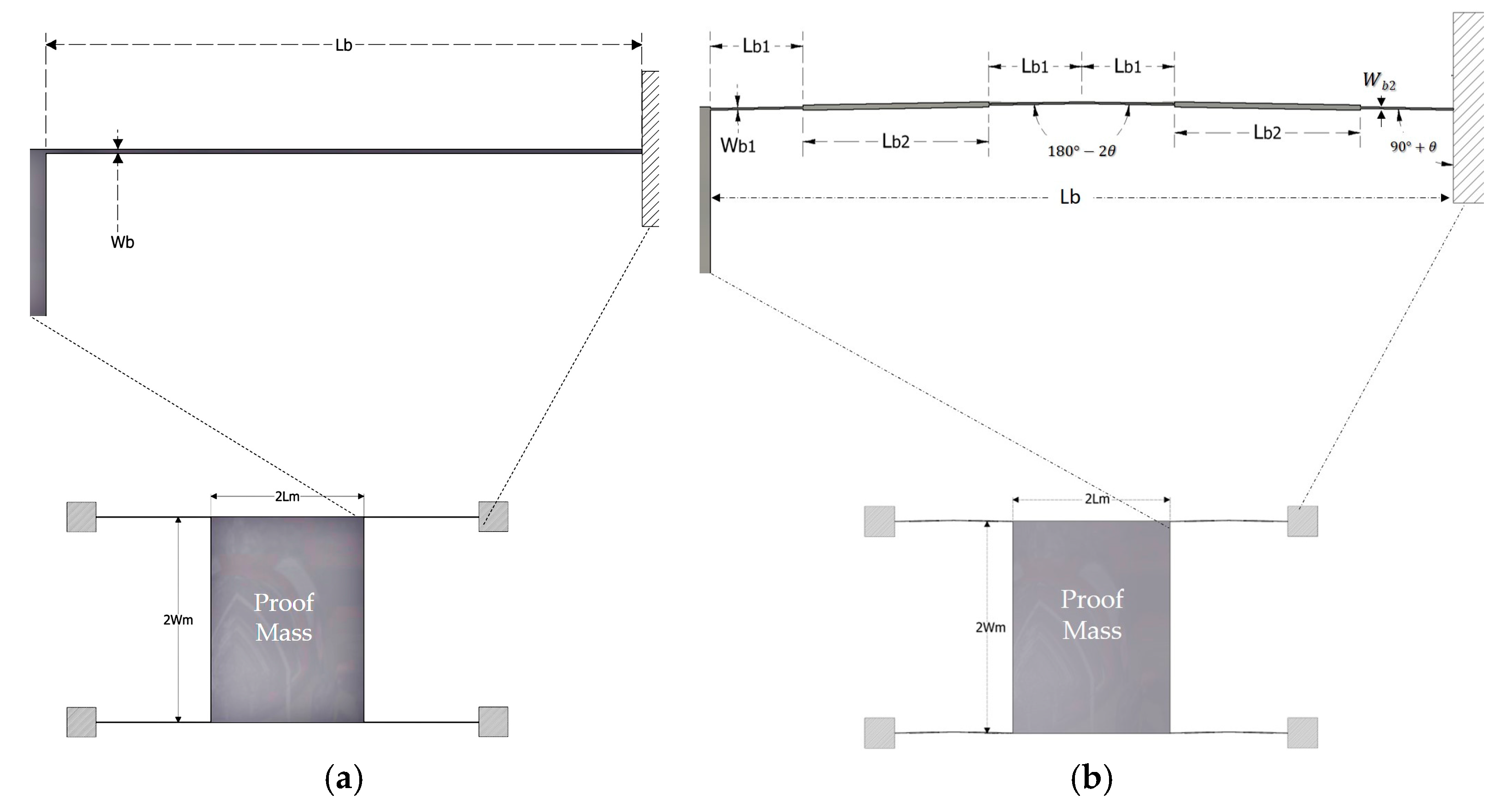
Complete accelerometer geometries with uniform and modified beams are shown in
Figure 3. Their main operation parameters are obtained by numerical analysis by the Finite Element Method (FEM).
Table 3 and
Table 4 show the material parameters and device dimensions, respectively.
3.1. Characteristic Equations for ¼ of Accelerometer with Symmetrical Beams
Total displacement is calculated by Equation (10), by adding the partial contributions of beam sections of lengths
Lb1 and
Lb2 (Equations (8) and (9)), multiplied by an adjustment factor (Δ). The equation of the maximum value of bending stress is given by Equation (13), where, again, it is given by the contributions of
Lb1 and
Lb2, multiplied by a correction factor (1.
τ), in accordance with the section of accelerometer under consideration (¼ or, ½,); 1.
τ corresponds to 1.25 or 1.5, respectively.
where
n corresponds to the number of elements
Lb1 and
Lb2. Analysis of the ¼ accelerometer with uniform beam is performed [
22].
3.2. Characteristic Equations for 1/2 of Accelerometer with Uniform Beams
The displacement is given by:
The second moment of inertia is provided by:
The maximum value of bending stress is given by:
3.3. Characteristic Equations for 1/2 of Accelerometer with Symmetrical Beams
In this case, Equations (8) to (12) are used, considering that Equations (14) and (15) must be used to calculate the moment of inertia and force, respectively. Total displacement for ½ accelerometer is given by:
3.4. Characteristic Equations for the Complete Accelerometer with Uniform Beams
Displacement, force and maximum value of bending stress in the complete accelerometer with uniform beams, are calculated as follows. From
:
Displacement
x(
yACC) can be obtained directly using Hooke’s Law.
Tmax is given by:
3.5. Characteristic Equations for Complete Accelerometer with Symmetrical Beams
For this case, Hooke equation and Equations (20) and (21) are used, considering the elements in the proposed beam shape:
where
N is the number of beams (L
b1) in the accelerometer, Δ is the adjustment factor = 10,
IWb1 and
IWb2 are the inertial moments of the corresponding beam width and
g is the gravity acceleration unit.
Tmax and the force
F of this accelerometer are calculated with Equations (2) and (18), respectively. Displacement is also obtained from Hooke’s Law.
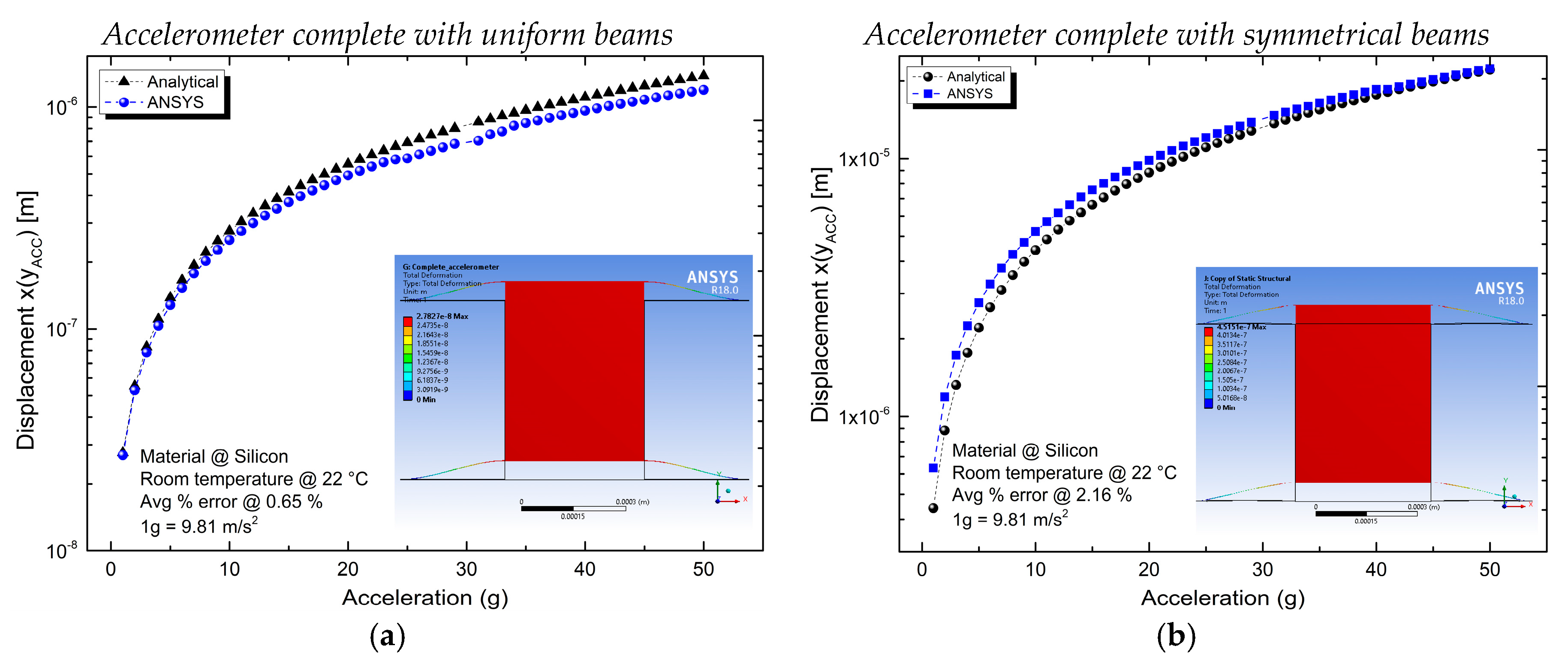
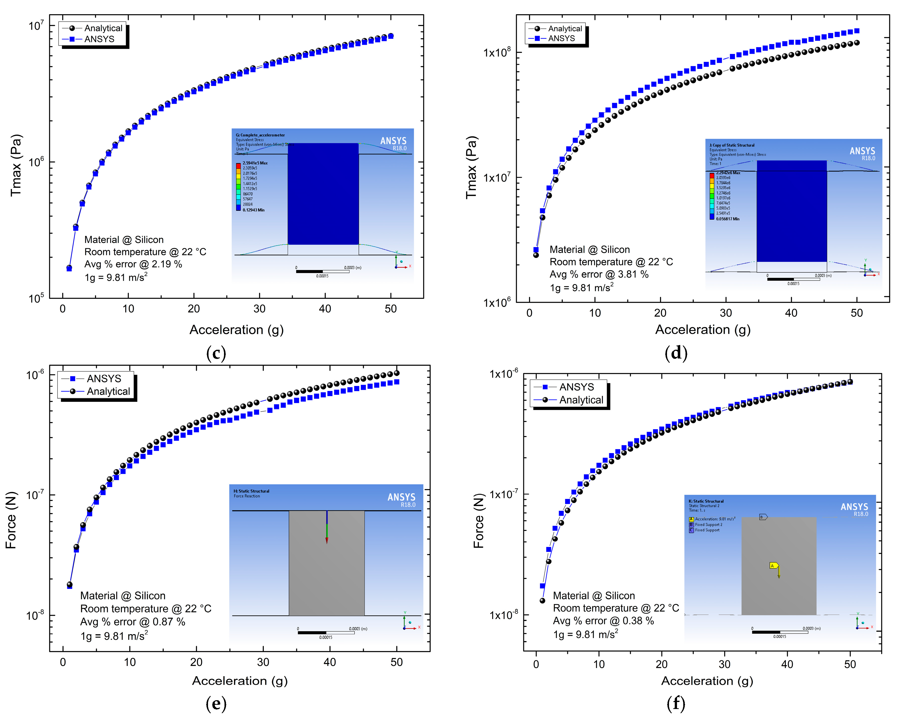
Table 5 provides the main parameter values for the case of ¼, ½ and complete conventional accelerometer with a uniform beam and with symmetrical beams. As can be observed, increments in displacement accelerometers with symmetrical beams are considerable. This high increment on displacement could be very useful when high sensitivity is required. Regarding force, for symmetrical accelerometers, their decrements are negligible. Simulation results for the case of complete accelerometers with uniform and symmetrical beams are shown in
Figure 4, as the representative case.
In
Table 5, the error between analytical and simulation values is also shown. As can be observed, for the ¼ accelerometer, the errors for all parameters are lower than 1%, while the largest error corresponds to the force. The highest range of errors corresponds to the ½ accelerometers, which increased from 0.98% (force parameter) to 11.89% (
Tmax). For the complete accelerometer, the largest error is 3.81% and corresponds to T
max. In
Figure 4, the average percentage of errors are also shown. For recurrence in two cases, an additional adjustment in T
max could be performed to decrease the error value. Differences between data from analytical and simulation are under an acceptable range. For the case of new analytical approximations, errors are obtained at larger values [
22].
Technical details about FEA analysis are provided in
Table 6.
To observe the effect of temperature on the natural frequency of both accelerometers, several temperatures were applied, from 22 to 1000 °C, without changes in the natural frequency’s values. A more detailed analysis could be performed in the future, with a thermal load and a complete system, considering that the vibrational property of cantilever beams relates the temperature change to their Young’s modulus [
26], and consequently to the spring constant.
Due to the proof mass made with a single material, the induced internal stress is equal to zero, as in [
13], producing no serious effect of temperature stress on the proof mass, subsequently increasing the robustness of the structure against temperature variations.
Table 7 provides data regarding individual the total constant stiffness of uniform and symmetrical beams, obtained from the number of beams in parallel considered in the arrangements (for ¼, ½ and complete accelerometer). Operation frequency is also provided. Decrements in stiffness are slow in all cases, considering as reference to the uniform one. Regarding frequency, decrements have larger values, from 24.8% up to 26.6%. The proposed accelerometer with symmetrical beams with this operating frequency values could be used in several applications with low-frequency requirements. All error values between simulations and analytical results are smaller than 11.89%. In [
22] and
Section 4.4, for new theoretical approximations of devices such as cantilevers, beams, springs, coils and accelerometers, larger error values than ours are reported.
To finish this section, the cross-axis sensitivities are given in
Table 8, for both accelerometers under analysis. As can be observed, these values are very small, indicating that the displacement on the Y-axis is considerably larger than the displacements on the other axes. The following equation was used for these calculations [
27]:
From the obtained results, it is observed that our main challenge was achieved, from the analysis of the spring–mass–damper system. The new geometry allows a larger displacement, with low values of cross-axis sensitivity, without the implementation of an additional amplifier of displacement.
4. Harmonic Response and Explicit Dynamic Analysis of the Devices
4.1. Harmonic Response Analysis
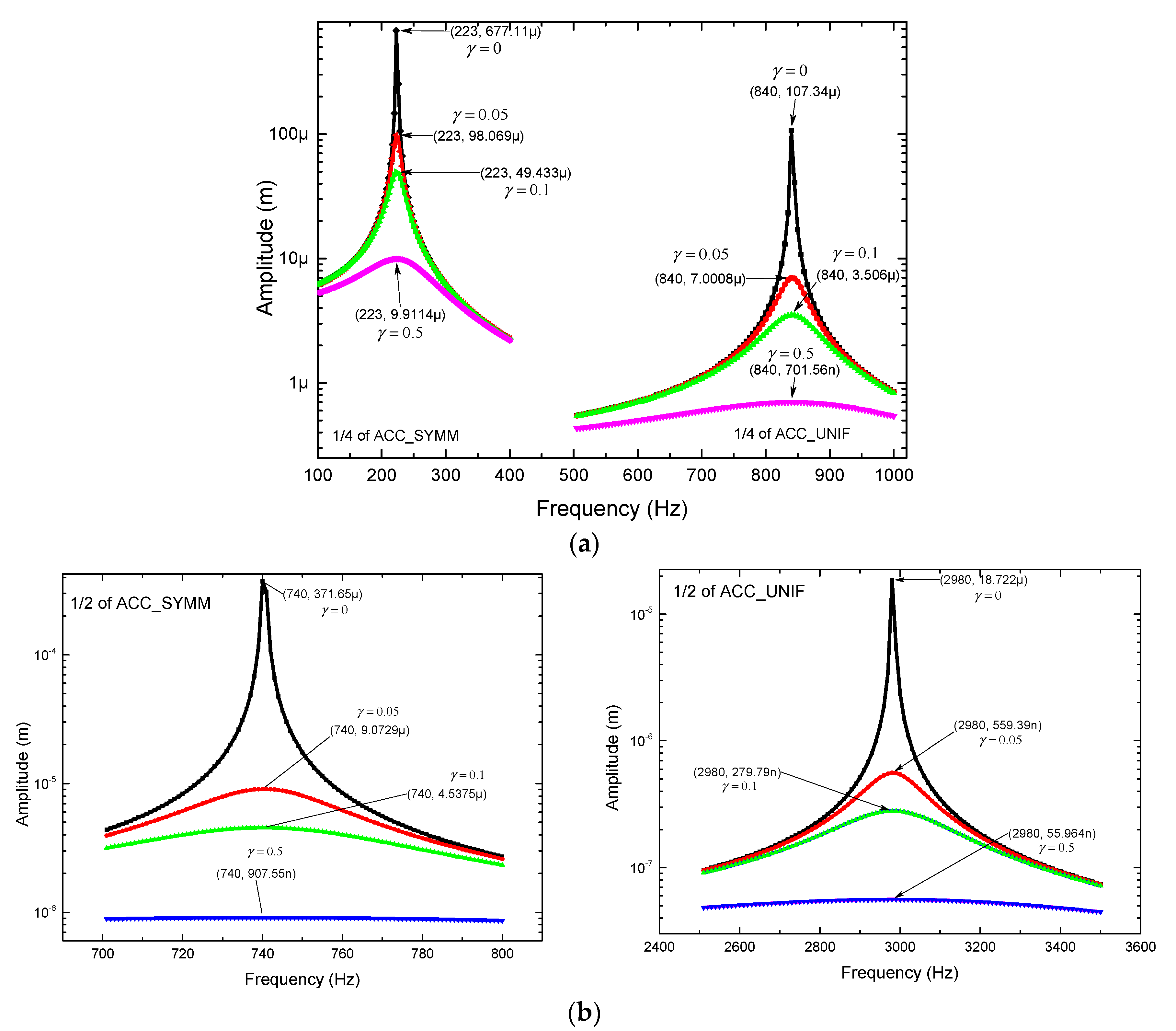
In this section, harmonic analysis will be developed by applying a structural load, considering normal operating conditions of devices. This fact allows us to obtain the effect of the transmissibility in each frequency, with the purpose of modifying or preventing those natural frequencies of the devices and reducing the effects of vibration in them. The cyclic loads on the accelerometers and their operating ranges are important aspects to consider in the devices’ structural design, as they allow the structural safety of all elements. A load of 1 g was assigned to all devices in the –Y-direction.
Table 9 shows the 10 modal forms of each device under analysis and the respective natural frequencies of the device. The characteristics and border conditions established in ANSYS were spacing linear frequency and a maximum frequency range of 600 kHz, with solution intervals of 100Hz and a full solution method.
Frequencies of the modal forms are in the following ranges: for the ¼ device with uniform arms, from 0.8 up to 491.74 kHz, and with symmetrical arms, from 0.22 up to 368.69 kHz; for the 1/2 device with uniform arms, from 1598 up to 273.84 kHz, and with symmetrical arms, from 0.74 up to 197.76 kHz; for complete accelerometers with uniform arms from 2.9 up to 179.23 kHz, and with symmetrical arms, from 0.74 up to 177.97 kHz. These frequency ranges allow us to obtain the harmonic response of the devices under a load, changing with time, to know if the structure supports dynamic loads, where the applied load produces a tangential pressure in the model, harmonically varying in the mentioned frequency range, as it can be observed in
Figure 5. For the evaluation, the results of the frequency response will be focused on the Y-direction. In each graph in
Figure 5, the maximum amplitude and its frequency represent the results of interest.
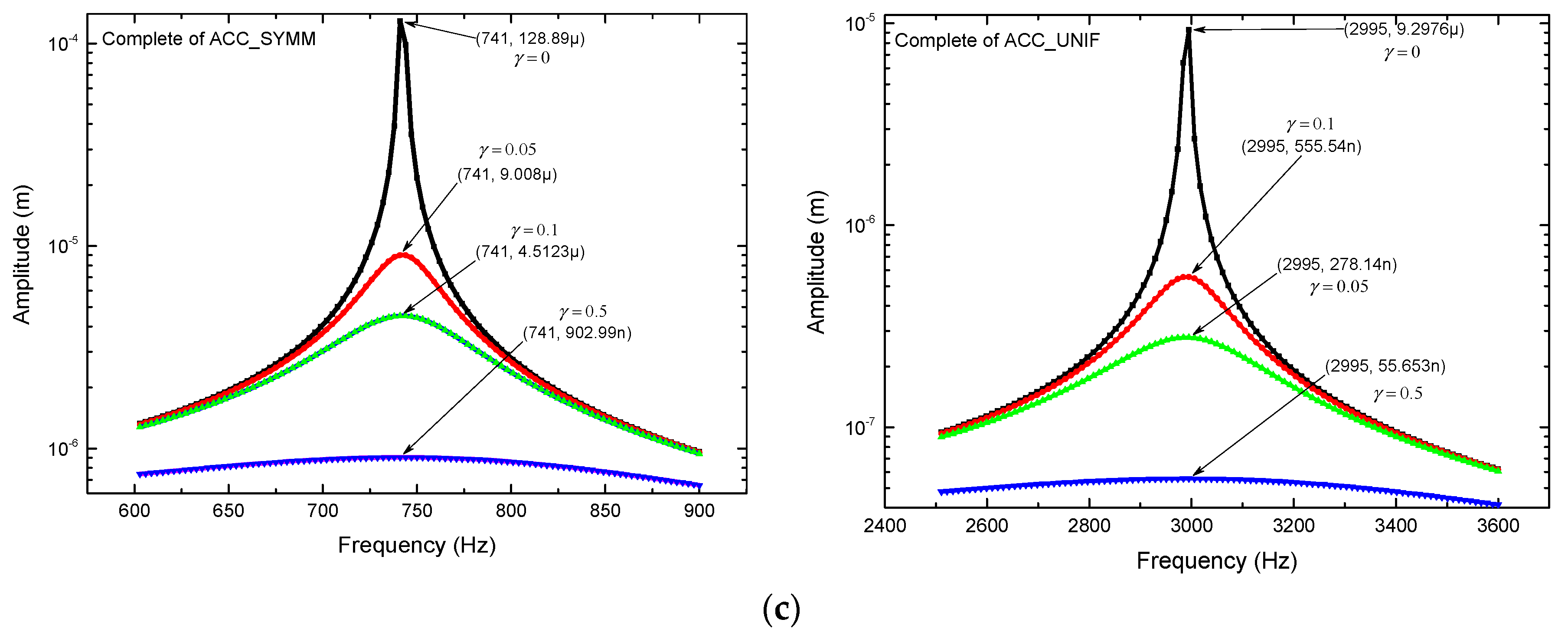
From
Figure 6, considering an appropriate bandwidth for the critical frequencies, obtained from
Figure 5, and applying a damping factor to the accelerometer, the values of stress are determined (See
Table 10). The corresponding amplitudes can be obtained directly from
Figure 6.
In
Table 11, technical details about FEA simulations considered in this section are given.
4.2. About the Damping Factor
The damping coefficient γ is the characteristic parameter of the damper. A damper dissipates energy and keeps the spring–mass system from vibrating forever. The ideal damper is considered to have no mass; thus, the force at one end is equal and opposite of the force at the other end [
28]. A representation is given in
Figure 1, in the basic mechanical mass–spring damper model. Relation with the quality factor was obtained from Equation (2):
Depending on the applications, γ may be too small for high-quality factor resonators, overdamped accelerometers and actuators, or something in between for gyroscopes [
22]. Sensors and actuators are typically close to critical damping. In microsystems, when adjusting the air pressure, the quality factor can be tailored over a wide range unless the microstructure is operating in vacuum. Modeling of the air damping is complex. The damping coefficient decreases with decreasing pressure.
In addition, the intrinsic material losses (internal friction) set the limit for the maximum quality factor for a given material. The material damping depends on the temperature, vibration frequency and vibration mode. Silicon has low intrinsic losses, which reduces its effect on the resonator performance.
The anchor losses can be much higher than the material loss limit especially for flexural structures, as in our case. When the device vibrates, a small portion of this energy leaks into the support, making important the location of the support point and the type of anchor. These differences are noted in simulation, when instead of a fixed-point anchor (to ensure that ideally, net stress in the anchor is zero), a complete anchor is considered.
In microscale, viscous losses due to fluid are often the dominant mechanisms. Several strategies to improve the performance of microdevices are given in [
22].
4.3. Explicit Dynamic Analysis
Explicit time integration is most accurate and efficient for simulations involving large deformations, and nonlinear buckling among other parameters. This method is used in the Explicit Dynamics analysis system, which calculates the response at the current time using explicit information. After meshing, in this case, the initial velocity is defined as the initial condition (
http://www.mechead.com/what-is-explicit-dynamics-in-ansys/).
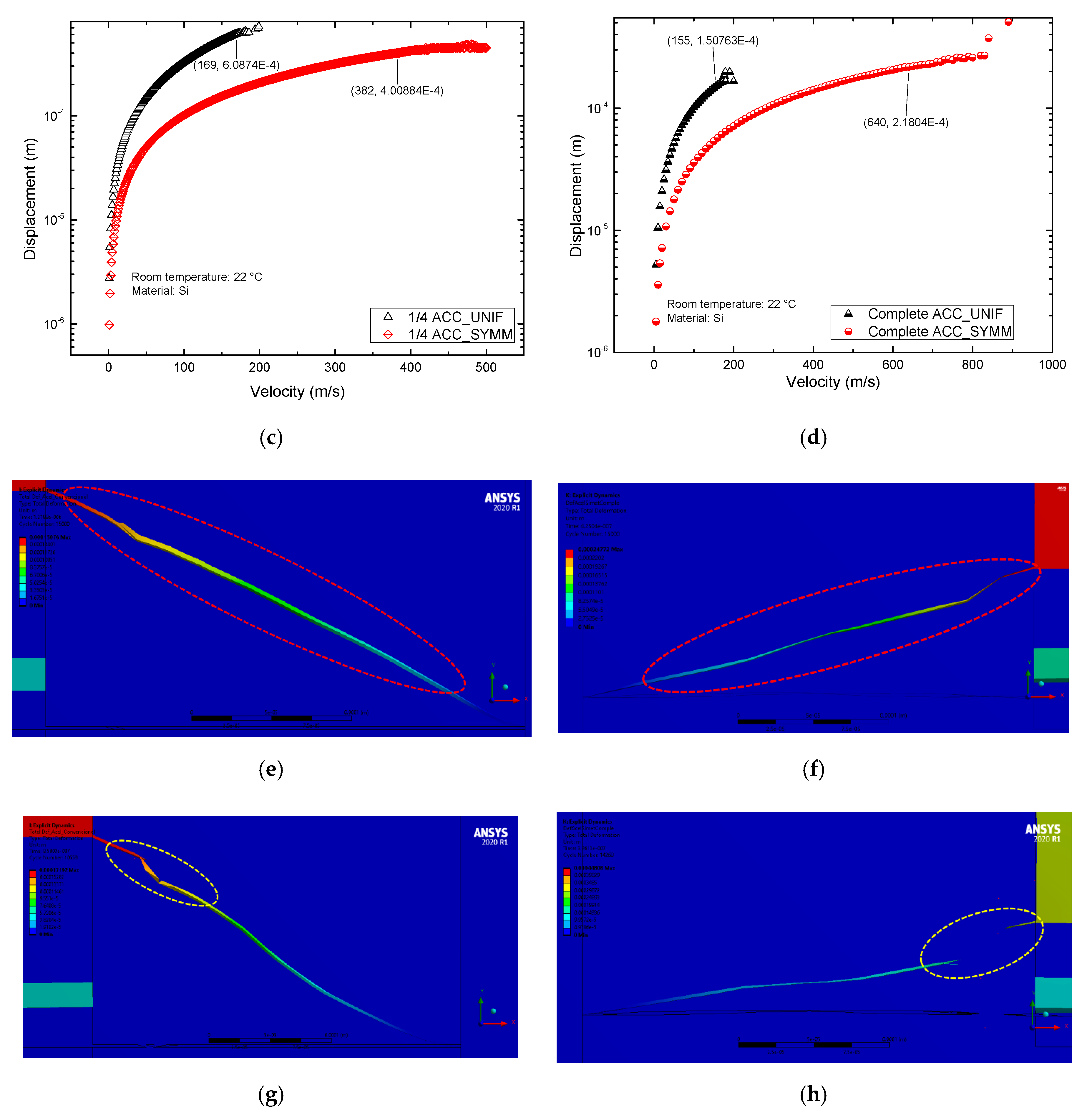
Figure 7 shows the response of ¼ and complete accelerometers, where it can be observed their performance, in terms of displacement, when velocity is applied. In both cases, it could be noted that accelerometers with uniform arms have faster response, but support smaller ranges of velocity. In
Figure 7a,b, representative figures of accelerometers inside a frame are given.
Figure 7c,d, shows their performance near to critical velocity values, while
Figure 7e,f, shows beams rupture at critical velocity values.
On the other hand, mechanical shock is a distributed force that can cause a system to vibrate after a drop, have a huge impact or even an explosion. It is known that MEMS devices, especially inertia sensors, can experience mechanical shock during fabrication, shipping, or storage processes [
29]. Those severe loads can cause stiction and even failure of the MEMS devices. With shock acceleration much larger than a sensing range, a mass moves excessively and a beam fractures when the maximum stress exceeds the critical stress of the beam. For this reason, high-shock accelerometers with a range of 1000 to 100,000 G are developed [
30]. A strategy to avoid this excessive movement of the mass [
28] is to improve shock resistance for both low-g and high-g accelerometers is to locate stoppers to limit the displacement of a mass. The effect of mechanical force on the proposed structure and a sweep of G values, bigger than 50G, applied to the proposed accelerometer could be performed in future work.
From our results (
Figure 7), with respect to the explicit dynamic analysis, it is possible to observe the increment of the shock resistance of the accelerometer with a symmetrical beam, larger than the case of the accelerometer with uniform beams, when they are subjected to velocity.
4.4. Comparison with Other Arm’s Shapes
In
Table 12, a comparison of the main parameters of three different geometries of accelerometers is performed. Each accelerometer is considered with its original uniform arms, and when they are replaced by the geometry here proposed, with and without angles in the determined junction points. For Accelerometer 1, the width of the uniform arm is of 40 μm, with the symmetric arms the increments in displacements are considerable with the proposed arms, especially for the case with angles; however, the natural frequency is reduced. For Accelerometers 2 (with a uniform arm width of 2.1 μm) and 3 (with a uniform arm width of 5 μm), with the symmetric arms, the case with angles only produces slight changes on all parameter values. In general, displacement increases considerably with the arm geometries proposed, producing an increment of the mechanical sensitivity of, on average, one order of magnitude. The force almost remains without change; the stress increases but remains much lower than the tensile yield strength value. Natural frequencies decrease in all cases. In summary, the influence of angles in symmetrical arms is significant only in the case of Accelerometer 1 [
31], especially for frequency response. It could be said that when proof mass is reduced, as well as the width of the corresponding arms, the effect of the angles could be neglected, as it happened in Accelerometers 2 and 3, due to the lower stiffness. Further analysis could be performed in future work.
4.5. Determination of Thinner Width Segments of Symmetrical Arms to Reduce the Natural Frequencies Decrement
In general, the increment in the displacement of proof mass implies a reduction in the natural frequency of accelerometers, representing a design compromise. In this case, we simulate the response of accelerometers when the width of the thinner segment is changed. Five cases were considered and reported in
Table 13, W
b2, as was previously defined, equal to the uniform arm width. As can be observed, for the first two cases, the increment in the displacement of the proof mass corresponds to increments from the reference by 24.82% and 39.57%, while the decrements in natural frequency are low, corresponding to 10.45% and 15.30%. Then these proportions are recommended for frequency values near to the case of uniform arms accelerometers, but with larger displacements. The changes in force are negligible, but the stress increases considerably, but far from critical values.
In order to observe the effect of bigger angles of the arms on the accelerometer with symmetric beams, a sweep of angle values is performed. The parameters of the symmetric accelerometer (W
b1 = (1/3) (W
b2)) are shown in
Table 14. The effect of angle changes on the main parameters is negligible. This fact represents an advantage for fabrication process selection.
A final test was performed considering two cases. The proposed symmetric beam geometry and a simplified variation, the last one only composed of a junction of two thinner segments, of width W
bu = W
b2/3, with angle θ = 1°. The simulation of stress is given in
Figure 8 for both cases. The zoom-in allows us to observe the place of the bigger stress in each case. The stress distribution is observed on all the thin guided segments of the symmetric beam (
Figure 8b), with the bigger value near to the proof mass. For the simplified case (uniform beams arrangement), the bigger stress values are located near to the proof mass (
Figure 8d), and on its corner, producing a small deformation on it. In this test, the lower effect on the corner of the proof mass is given with the symmetric beam. The advantage of the symmetric beam is the stress distribution, reducing its effect on the proof mass.
4.6. Nonlinearities
The proposed symmetric beam model is linear. As it is described in [
33], geometric nonlinearities can appear in any mechanical structure when large deformations induce a nonlinear relation between strain and curvature, thus modifying the effective stiffness of the structure (i.e., elastoplastic material). The effect of nonlinearity is found to be significant when the deflection of the microbeam exceeds 30% of its length [
29]. For the proposed beam in this paper, the deflections are smaller than the total length for frequencies lower than the first modal frequency, with damping factor different to zero (
Figure 6c).
On the other side, it is important to mention that monitoring the displacement of microelectromechanical resonators oscillating in the linear regime (where the vibration amplitude of the resonator is lower than the critical amplitude) may be difficult without a displacement detector with high sensitivity [
34] because the signals may be weak [
35]. The nonlinear effects are of great importance, and in many cases, are the only useful regime of operation, as only relatively small applied forces are needed for driving a micromechanical oscillator into a nonlinear regime. Rate of damping is another key property of systems based on mechanical oscillators.
In addition, material nonlinearity (response to temperature, pressure, among other variables) and fabrication uncertainties such as surface roughness, clamping variations, surface damage, fabrication residues etc., could lead to deviations in the device dimensions and material properties, which, in turn, could affect the overall nonlinear response. To minimize these effects, it is desirable to account for an adequate fabrication process.
Boundary conditions have also been identified as a source of nonlinearity. For example, in [
22], it is recognized that the analytical approximations and FEM model are based on somewhat unrealistic fixed boundary conditions. The anchors could generally bend, stretch and move. In addition, the Degree of Freedom (DOF) could also be restricted.
It is well known that in the first estimate, linear static analysis is often used prior to performing a full nonlinear analysis. Then, there are several details to consider in future work about the proposed device.
5. Conclusions
For the ¼, ½ and complete accelerometers, implemented with the proposed symmetrical beam shape, equations of displacement and force were developed. The error of the analytical approximations compared with simulation results are in an acceptable range. Equations for maximum stress value are similar in all analyzed cases to accelerometers with the uniform beam.
The implementation of symmetrical beams in the ¼, ½ and complete accelerometers provides a notable increase in deformation at the corresponding guided ends, compared with the cases with uniform beams, achieving the objective of this work. These results are a consequence of the reduction of the stiffness constant, due to the mass distribution and by the angular beam arrangement.
The operation frequency for the ¼, ½ and complete accelerometer with symmetrical beams, however, is always reduced. The decrements of force in all cases are negligible.
The proposed accelerometer could be used in low-frequency applications such as seismometer, measurements of tides, among others. In the detection of seizure-associated high-frequency oscillations, due to high-frequency oscillations in the electroencephalograms of epileptic patients have been studied in the frequency range of up to 800 Hz [
36].
In the case of accelerometers with symmetrical beams, locations of the maximum values of normal stress are found at the guided ends. In their middle parts, median valor of stress is also shown. In all cases, the maximum normal stress values are considerably lower than the tensile yield strength, which is necessary for structural integrity. The transfer of stress to the proof mass is reduced for the case of symmetrical beams compared with the uniform case.
Harmonic analysis allows us, from the modal form’s frequencies, to determine maximum amplitudes and the corresponding frequency ranges of the accelerometer’s response at 1 g. Explicit analysis lets us know the maximum velocities supported for each device under analysis. In this case, an accelerometer with symmetrical arms can support bigger velocities than the rectangular one, showing the largest shock resistance under this condition.
In addition, from variation in the width of the thinner segment of the symmetrical arms, it can be observed that it is possible to obtain an increment in the displacement of the proof mass of 39.57%, with a decrement in natural frequency of 15.30%, taking as reference the response of the accelerometer with uniform beam, which is found as a useful result and avoids the use of an additional mechanical amplifier.
By replacing the symmetrical beams by the uniform ones in three capacitive accelerometers, an increment, on average, of one order magnitude was obtained on the displacement sensitivity. It is a clear advantage of the proposed geometry.
Other advantages of the symmetric beam are the stress distribution, reducing its effect on the proof mass, as well as their low cross-axis sensitivity.
The beam shape optimization is identified as future work. It is also necessary to derive design rules for performance enhancement of MEMS accelerometers. A study of temperature effects on the accelerometer performance is also an identified future task.
Author Contributions
Conceptualization, investigation and funding acquisition, M.T.-T.; formal analysis, writing—original draft preparation and editing, P.V.-C. and M.T.-T.; software, methodology and validation, P.V.-C., and R.C.-R.; resources and investigation, M.T.-T., P.V.-C., J.O.S.-R. and S.F.R.-F. All authors have read and agreed to the published version of the manuscript.
Funding
This research was funded by CONACyT, grant number A1-S-33433, “Proyecto Apoyado por el Fondo Sectorial de Investigación para la Educación”.
Acknowledgments
Josue Osvaldo Sandoval-Reyes is grateful for the support of CONACYT, for his doctoral studies scholarship, under grant 782822.
Conflicts of Interest
The authors declare no conflict of interest.
References
- Mezghani, B.; Tounsi, F.; Masmoudi, M. Convection behavior analysis of CMOS MEMS thermal accelerometers using FEM and Hardee’s model. Analog. Integr. Circuits Signal Process. 2013, 78, 301–311. [Google Scholar] [CrossRef]
- MEMS Applications Overview. MEMS Applications PK, MEMS Applications Activity. Participant Guide; Southwest Center for Microsystems Education. SCME. Available online: http://nanotechradar.com/sites/default/files/inano10_mems_applications_overview.pdf (accessed on 15 October 2019).
- Girish, K.; Chaitanya, U.; Kshisagar, G.K.; Ananthasuresh, N.B. Micromachines hgh-resolution accelerometers. J. Indian Inst. Sci. 2007, 87, 333–361. [Google Scholar]
- Tavakkoli, H.; Momen, H.G.; Sani, E.A.; Yazgi, M. An Inductive MEMS Accelerometer. In Proceedings of the 10th International Conference on Electrical and Electronics Engineering (ELECO), Bursa, Turkey, 30 November–2 December 2017; pp. 459–463. [Google Scholar]
- Andrejasic, M. MEMS Accelerometers Seminar, University of Ljubljana. Marec. 2008. Available online: http://mafija.fmf.uni-lj.si/seminar/files/2007_2008/MEMS_accelerometers-koncna.pdf (accessed on 16 January 2020).
- Liu, Y.; Wang, H.; Qin, H.; Zhao, W.; Wang, P. Geometry and Profile Modification of Microcantilevers for Sensitivity Enhancement in Sensing Applications. Sens. Mater. 2017, 29, 1. [Google Scholar] [CrossRef]
- Graak, P.; Gupta, A.; Kaur, S.; Chhabra, P.; Kumar, D.; Shetty, A. Simulation of Various Shapes of Cantilever Beam for Piezoelectric Power Generator. In Proceedings of the 2015 COMSOL Conference, Pune, India, 29 October 2015. [Google Scholar]
- Hawari, H.F.; Wahab, Y.; Azmi, M.T.; Shakaff, A.Y.M.; Hashim, U.; Johari, S. Design and Analysis of Various Microcantilever Shapes for MEMS Based Sensing. J. Phys. Conf. Ser. 2014, 495, 012045. [Google Scholar] [CrossRef]
- Siddaiah, N.; Prasad, G.R.K.; Asritha, K.; Hanumanthu, P.V.; Anvitha, N.; Chandra Sekhar, T.N.V. Design and model analysis of various shape cantilever-based sensors for biomolecules detection. J. Adv. Res. Dyn. Control Syst. 2017, 9, 476–485. [Google Scholar]
- Parsediya, D.K.; Singh, J.; Kankar, P.K. Simulation and Analysis of Highly Sensitive MEMS Cantilever Designs for “in vivo Label Free” Biosensing. In Proceedings of the 2nd International Conference on Innovations in Automation and Mechatronics Engineering (ICIAME), Vallabh Vidyanagar, India, 7–8 March 2014; pp. 85–92. [Google Scholar]
- Zhou, X.; Che, L.; Liang, S.; Lin, Y.; Li, X.; Wang, Y. Design and fabrication of a MEMS capacitive accelerometer with fully symmetrical double-sided H-shaped beam structure. Microelectron. Eng. 2015, 131, 51–57. [Google Scholar] [CrossRef]
- Solai, K.; Rathnasami, J.D.; Koilmani, S. Superior performance area changing capacitive MEMS accelerometer employing additional lateral springs for low frequency applications. Microsyst. Technol. 2020, 26, 1–18. [Google Scholar] [CrossRef]
- Yamane, D.; Konishi, T.; Safu, T.; Toshiyoshi, H.; Sone, M.; Machida, K.; Ito, H.; Masu, K. A MEMS Accelerometer for Sub-mG Sensing. Sens. Mater. 2019, 31, 2883. [Google Scholar] [CrossRef]
- Keshavarzi, M.; Hasani, J.Y. Design and optimization of fully differential capacitive MEMS accelerometer based on surface micromachining. Microsyst. Technol. 2018, 25, 1369–1377. [Google Scholar] [CrossRef]
- Xiao, D.B.; Li, Q.S.; Hou, Z.Q.; Wang, X.H.; Chen, Z.H.; Xia, D.W.; Wu, X.Z. A novel sandwich differential capacitive accelerometer with symmetrical double-sided serpentine beam-mass structure. J. Micromech. Microeng. 2015, 26, 025005. [Google Scholar] [CrossRef]
- Xu, W.; Yang, J.; Xie, G.; Wang, B.; Qu, M.; Wang, X.; Liu, X.; Tang, B. Design and Fabrication of a Slanted-Beam MEMS Accelerometer. Micromachines 2017, 8, 77. [Google Scholar] [CrossRef]
- Avinash, K.; Siddheshwar, K. Comparative Study of Different Flexures of MEMS Accelerometers. Int. J. Eng. Adv. Technol. 2015, 4, 2249–8958. [Google Scholar]
- Benevicius, V.; Ostasevicius, V.; Gaidys, R. Identification of Capacitive MEMS Accelerometer Structure Parameters for Human Body Dynamics Measurements. Sensors 2013, 13, 11184–11195. [Google Scholar] [CrossRef] [PubMed]
- Aoyagi, S.; Makihira, K.; Yoshikawa, D.; Tai, Y. Parylene Accelerometer Utilizing Spiral Beams. In Proceedings of the 19th IEEE International Conference on Micro Electro Mechanical Systems, Istanbul, Turkey, 22–26 January 2006. [Google Scholar]
- Benmessaoud, M.; Nasreddine, M.M. Optimization of MEMS capacitive accelerometer. Microsyst. Technol. 2013, 19, 713–720. [Google Scholar] [CrossRef]
- Van Kampen, R.; Wolffenbuttel, R. Modeling the mechanical behavior of bulk-micromachined silicon accelerometers. Sens. Actuators A Phys. 1998, 64, 137–150. [Google Scholar] [CrossRef]
- Kaajakari, V. Practical MEMS; Small Gear Publishing: Las Vegas, NV, USA, 2009; ISBN 978-0-9822991-0-4. [Google Scholar]
- William, F.R.; Sturges, L.D.; Morris, D.H. Mecánica de Materiales Limusa; Wiley: Mexico City, Mexico, 2001. [Google Scholar]
- Yang, S.; Xu, Q. A review on actuation and sensing techniques for MEMS-based microgrippers. J. Micro Bio Robot. 2017, 13, 1–14. [Google Scholar] [CrossRef]
- Kuo, J.-C.; Huang, H.-W.; Tung, S.-W.; Yang, Y.-J. A hydrogel-based intravascular microgripper manipulated using magnetic fields. Sens. Actuators A Phys. 2014, 211, 121–130. [Google Scholar] [CrossRef]
- Toda, M.; Inomata, N.; Ono, T.; Voiculescu, I. Cantilever beam temperature sensors for biological applications. IEEJ Trans. Electr. Electron. Eng. 2017, 12, 153–160. [Google Scholar] [CrossRef]
- Sankar, A.R.; Jency, J.G.; Das, S. Design, fabrication and testing of a high performance silicon piezoresistive Z-axis accelerometer with proof mass-edge-aligned-flexures. Microsyst. Technol. 2011, 18, 9–23. [Google Scholar] [CrossRef]
- Piersol, A.G.; Paez, T.L. Harri´s Shock and Vibration Handbook, 6th ed.; Blake, R.E., Ed.; McGraw Hill: New York, NY, USA, 2010; Chapter 2. [Google Scholar]
- Ouakad, H.M. The response of a micro-electro-mechanical system (MEMS) cantilever-paddle gas sensor to mechanical shock loads. J. Vib. Control. 2013, 21, 2739–2754. [Google Scholar] [CrossRef]
- Kazama, A.; Aono, T.; Okada, R. High Shock-Resistant Design for Wafer-Level-Packaged Three-Axis Accelerometer with Ring-Shaped Beam. J. Microelectromech. Syst. 2018, 27, 355–364. [Google Scholar] [CrossRef]
- Koberstein, L.L.; Fonseca, F.J.; Fraga, M.A.; Rasia, L.A. Optimized Design of a Bridge Type Accelerometer. In Proceedings of the IBERSENSOR, Montevideo, Uruguay, 27–29 September 2006; pp. 1–6, ISBN 9974-0-0337-7. [Google Scholar]
- Karthikeyan, K.; Xingguo, X.; Linfeng, Z.; Junling, H. Fault Simulation of Surface-Micromachined MEMS Accelerometer. In Proceedings of the ASEE (The American Society for Engineering Education) Conference, Bridgeport, CN, USA, 3–4 April 2009; pp. 1–7. [Google Scholar]
- Villanueva, L.G.; Karabalin, R.B.; Matheny, M.H.; Chi, D.; Sader, J.E.; Roukes, M.L. Nonlinearity in nanomechanical cantilevers. Phys. Rev. B 2013, 87, 024304. [Google Scholar] [CrossRef]
- Zaitsev, S.; Shtempluck, O.; Buks, E.; Gottlieb, O. Nonlinear damping in a micromechanical oscillator. Nonlinear Dyn. 2011, 67, 859–883. [Google Scholar] [CrossRef]
- Kacem, N.; Hentz, S.; Pinto, D.; Reig, B.; Nguyen, V. Nonlinear dynamics of nanomechanical beam resonators: Improving the performance of NEMS-based sensors. Nanotechnology 2009, 20, 275501. [Google Scholar] [CrossRef] [PubMed]
- Kobayashi, K.; Agari, T.; Oka, M.; Yoshinaga, H.; Date, I.; Ohtsuka, Y.; Gotman, J. Detection of seizure-associated high-frequency oscillations above 500Hz. Epilepsy Res. 2010, 88, 139–144. [Google Scholar] [CrossRef] [PubMed][Green Version]
Figure 1.
(a) Typical capacitive accelerometer with uniform flexures. (b) Basic mechanical mass–spring damper model.
Figure 1.
(a) Typical capacitive accelerometer with uniform flexures. (b) Basic mechanical mass–spring damper model.
Figure 2.
Cantilever spring.
Figure 2.
Cantilever spring.
Figure 3.
Frontal view of accelerometer: (a) uniform beam and (b) symmetrical beam.
Figure 3.
Frontal view of accelerometer: (a) uniform beam and (b) symmetrical beam.
Figure 4.
Simulated parameter values of the complete accelerometers with uniform and symmetrical beams, respectively, considering a sweep on applied acceleration from 1 to 50 g. (a,b) Displacement of guided ends. (c,d) Maximum stress at clamped ends of beams. (e,f) Force applied to the guided end.
Figure 4.
Simulated parameter values of the complete accelerometers with uniform and symmetrical beams, respectively, considering a sweep on applied acceleration from 1 to 50 g. (a,b) Displacement of guided ends. (c,d) Maximum stress at clamped ends of beams. (e,f) Force applied to the guided end.
Figure 5.
Harmonic response of devices: (a) ¼ of ACC_UNIF and ¼ of ACC_SYMM, (b) ½ of ACC_UNIF and ½ of ACC_SYMM and (c) Complete ACC_UNIF and Complete of ACC_SYMM.
Figure 5.
Harmonic response of devices: (a) ¼ of ACC_UNIF and ¼ of ACC_SYMM, (b) ½ of ACC_UNIF and ½ of ACC_SYMM and (c) Complete ACC_UNIF and Complete of ACC_SYMM.
Figure 6.
Harmonic response of devices with damping factor (γ): (a) ¼ of ACC_SYMM and ¼ of ACC_UNIF. (b) ½ of ACC_SYMM and ½ of ACC_UNIF. (c) Complete ACC_SYMM and Complete ACC_UNIF.
Figure 6.
Harmonic response of devices with damping factor (γ): (a) ¼ of ACC_SYMM and ¼ of ACC_UNIF. (b) ½ of ACC_SYMM and ½ of ACC_UNIF. (c) Complete ACC_SYMM and Complete ACC_UNIF.
Figure 7.
Explicit dynamic analysis. Velocity applied to (a) ¼ of ACC_SYMM, 3D view. (b) Complete ACC_SYMM, 3D view. Displacement of (c) ¼ of ACC_SYMM and ¼ of ACC_UNIF, (d) Complete ACC_SYMM and Complete ACC_UNIF. Performance with velocity load at (e) 155 m/s for Complete ACC_UNIF, and (f) 640 m/s for Complete ACC_SYMM. Performance of (g) complete ACC_UNIF at 250 m/s and (h) Complete ACC_SYMM at 1 km/s.
Figure 8.
Simulation of stress for (a) the accelerometer with symmetric beams, (b) zoom in at one of the symmetric beams, (c) accelerometer with simplified beams and (d) zoom in at the one of the simplified beams.
Figure 8.
Simulation of stress for (a) the accelerometer with symmetric beams, (b) zoom in at one of the symmetric beams, (c) accelerometer with simplified beams and (d) zoom in at the one of the simplified beams.
Table 1.
Beam shapes and cantilevers.
Table 1.
Beam shapes and cantilevers.
| Ref. | Year | Shape of Beams | Material | Larger Displacement and Conditions | Stress | Natural Freq. |
|---|
| Authors | Beam Size (µm × µm × µm) |
|---|
| [7] | 2015 | E, pi and T | Silicon/PZT-5H. | 0.6078 µm,
E-shaped beam
(applied force: 0.5 µN). | N/A | N/A |
| P. Graak et al. | 60 × 10 × (1.5/0.5) |
| [8] | 2014 | Trapezoid and rectangular, double- and single-legged | Silicon | 6.93 × 10⁻⁴ µm,
one legged-rectangular beam (constant force applied). | 20.361 MPa | 11.58 MHz |
| H. F. Hawari et al. | 110 × 50 × 40 |
| [9] | 2017 | Basic, T and circular | Si, Ge, Ni, SiO2, PMMA, polymide | Disk-shaped cantilever of silicon (load of 1 kg/m2). It is followed by T-shaped. | N/A | Max. Eigenfrequency = 0.498.94 MHz |
| Siddaiah et al. | 80 × 20 |
| [10] | 2014 | Trapezoidal, trapezoidal with square step at fixed end, length-wise symmetry | SiO2 over Si | 0.231 × 10⁻⁹ m, Trapezoidal with square step at fixed end (pressure 19.2 Pa, equal to surface stress 0.05 N/m). | N/A | N/A |
| Parsediya et al. | 50, 50 and 150, t = 50. Trapezoidal with square step at fixed end |
Table 2.
Accelerometers with different beam shapes.
Table 2.
Accelerometers with different beam shapes.
| Ref. | Year | Shape of Beams | Material | Larger Displacement | Stress | Natural Freq. |
|---|
| Authors | Mass and
Beam Sizes
(µm × µm × µm) |
|---|
| Capacitive Sandwiched Accelerometers |
| [11] | 2015 | Fully symmetrical double-sided H-shaped | 3 silicon wafers | N/A | N/A | 1.954 kHz |
| Xiaofeng Zhou et al. | Mass: 3200 × 3200 × 560
Beam: 380 × 20 × 30 |
| [15] | 2016 | Symmetrical double-sided serpentine | Glass–silicon–glass | 0.574 μm on Z-axis, at 1 g | N/A | N/A |
| D. B. Xiao et al. | Proof Mass: 4 × 4mm ×
Beam: total length 8.4 mm w of each beam: 0.14 mm,
t = 25 µm |
| [16] | 2017 | Slanted beams | Glass–silicon–glass | 0.632 μm at 50 g | N/A | 3.9 kHz |
| Wei Xu et al. | Proof mass: 2100 × 1800 × 380
Slanted beam: 1000 × 380 × 120 |
| Capacitive Accelerometers |
| [17] | 2015 | Straight-, crab-leg, serpentine and folded | Silicon | 0.3 μm | N/A | 6.842 MHz
Crab-leg flexure |
| Avinash and Siddheshwar | Proof mass: 540 × 400 × 2.1
Crab-leg Beam:
300 × 150. All structure thickness: 3.5 |
| [18] | 2013 | L-shaped beams | Proof mass of Cu, beams of Si | In z, 50.55 nm at 10 m/s2 | N/A | In z, 1st eigenfreq 2254.42
Hz |
| Vincas Benevicius et al. | Proof mass: 100 × 100 × 100
Beams, cross size: 5 × 8.25
Overall size 1.23 × 1.23 mm |
| [19] | 2006 | Spiral beams | Parylene | N/A | <5 MPa
(spiral structure) | 0.5 kHz |
| S. Aoyagi et al. | Proof mass r = 1000, t = 5
Beam 1800 × 100 × 5 |
| [13] | 2019 | Multilayer metal serpentine springs | Au proof mass,
Si beams | N/A | N/A | 202 Hz at 0.5 V (DC Vias V) |
| Daisuke Yamane et al. | Mass 4000 × 4000 × 20
Beam (Lb × La × W × t): 200 × 10 × 6 × 15 |
| [12] | 2020 | Folded beams | Silicon | 148 μm at 1 g, in X-axis, Beam
t = 5 μm | | 100 Hz |
| Kannan Solai et al. | Proof mass with parallel plates: 3000 × 5000 × 80
Beams (Lb × Wb × La): 1800 × 4 × 100 |
| [14] | 2018 | π-shaped springs (fully differential capacitive MEMS
accelerometer) | Silicon | 29.8 nm at 1 g, 300 nm at 10 g | N/A | 2870 Hz (1st frequency mode) |
| Keshavarzi and Hasani | Differential sensor (L × W) 1 × 1mm
Beam (L × W × t) 160 × 2 × 10 |
| [20] | 2013 | Folded beams with turns (comb accel.) | PolySi | 0.5 μm at 1 g and Wb = 2 μm | N/A | N/A |
| Benmessaoud M. et al. | Mass: 80 × 200
Beam: 270 × 3
Variation of thickness |
Table 3.
Mechanical properties of silicon.
Table 3.
Mechanical properties of silicon.
| Parameters and Units | Silicon [24,25] |
|---|
| Density, ρ (kg/m3) | 2329 |
| Young’s modulus, E (GPa) | 130.1 |
| Coefficient of thermal expansion, α ((1/°K)) | 2.568 × 10⁻⁶ |
| Poisson ratio, ν (dimensionless) | 0.33 |
| Tensile yield strength (MPa) | 250 |
Table 4.
Dimensions of mass and uniform and proposed modified beams.
Table 4.
Dimensions of mass and uniform and proposed modified beams.
| ID | Description | Dimensions (µm) |
|---|
| Lm | Length of the roof mass of the ¼ accelerometer | 200 |
| Wm | Width of the proof mass of the ¼ accelerometer | 270 |
| Lb | Length of the uniform cantilever | 300 |
| Wb | Width of the uniform cantilever | 2.1 |
| t | Device thickness | 3.5 |
| Lm/2 | Center of the gravity for the mass | 100 |
| Lb1 | Length of the 1st, 3rd, 4th and 6th sections of the proposed beam | Lb/8 = 37.5 |
| Lb2 | Length of the 2nd and 5th sections of the proposed beam | 2 (Lb/8) =75 |
| θ | Inclination angle | 1° |
| Wb2 | Width of sections with Lb2 | Wb = 2.1 |
| Wb1 | Width of sections with Lb1 | Wb/3 = 0.7 |
Table 5.
Parameters of the ¼ accelerometer with uniform and symmetrical beams at 1 g.
Table 5.
Parameters of the ¼ accelerometer with uniform and symmetrical beams at 1 g.
| Parameters | Analytical Value | Value ANSYS | Avg. Error% | Analytical Value | Value ANSYS | Avg. Error% |
|---|
| | ¼ of accelerometer, uniform beams (ACC_UNIF) | ¼ of accelerometer symmetrical beams (ACC_SYMM) |
| x(yτ) = x(y1/4) Deformation, (µm) | 0.1659 | 0.166 | 0.03 | 2.372 | 2.382 | 0.421 |
| Tmax (stress, MPa) | 0.5036 | 0.501 | 0.47 | 4.09 | 4.058 | 0.82 |
| Force (nN) | 4.32 | 4.34 | 0.58 | 4.318 | 4.359 | 0.94 |
| | 1/2 ACC_UNIF | 1/2 ACC_SYMM |
| x(yτ) = x(y1/2) Deformation, (µm) | 0.0311 | 0.0279 | 10.04 | 0.4447 | 0.4538 | 2.04 |
| Tmax (stress, MPa) | 0.1888 | 0.1664 | 11.89 | 2.4 | 2.31 | 3.41 |
| Force (nN) | 8.6364 | 8.6865 | 0.58 | 8.636 | 8.6699 | 0.94 |
| | Complete ACC_UNIF | Complete ACC_SYMM |
| x(ycomplete) Deformation, (µm) | 0.0277 | 0.0278 | 0.65 | 0.441 | 0.451 | 2.16 |
| Tmax (stress, MPa) | 0.1259 | 0.1642 | 2.19 | 2.38 | 2.29 | 3.81 |
| Force (nN) | 17.27 | 17.42 | 0.87 | 17.27 | 17.38 | 0.38 |
Table 6.
Technical details about Finite Element Analysis (FEA).
Table 6.
Technical details about Finite Element Analysis (FEA).
| Device | Solver Target | Element Type/Mesh | Convergence | Total Mass (kg) |
|---|
| No. of Total Nodes | No. of Total Elements | Change % |
|---|
| ¼ of accelerometer, uniform beams (ACC_UNIF) | Mechanical APDL | SOLID 187/Refinement
Controlled program (Tet10) | 12,241 | 5920 | 0.20869 | 0.44532 × 10⁻⁹ |
| ¼ of accelerometer symmetrical beams (ACC_SYMM) | 11,825 | 5562 | 0.28611 | 0.4436 × 10⁻⁹ |
| 1/2 ACC_UNIF | 16,821 | 7978 | 0.3232 | 0.89063 × 10⁻⁹ |
| 1/2 ACC_SYMM | 22,807 | 11,275 | 0.20715 | 0.88721 × 10⁻⁹ |
| Complete ACC_UNIF | 23,737 | 11,739 | 0.49405 | 1.7813 × 10⁻⁹ |
| Complete ACC_SYMM | 46,237 | 24,129 | 0.54386 | 1.7744 × 10⁻⁹ |
Table 7.
Stiffness constant of uniform and symmetrical beams and operation frequency of the ¼, ½ and complete accelerometers.
Table 7.
Stiffness constant of uniform and symmetrical beams and operation frequency of the ¼, ½ and complete accelerometers.
| Parameters | Fraction of UNIF Beam ACC, ANSYS | Fraction of SYMM Beam ACC, ANSYS | Decrement
% |
|---|
| | ¼ of ACC_UNIF | ¼ of ACC_SYMM | |
| Stiffness constant of the spring, N/m | 2.62 × 10⁻² | 1.83 × 10⁻³ | 6.98 |
| Natural frequency, Hz | 841.37 | 223.84 | 26.6 |
| | ½ of ACC_UNIF | ½ of ACC_SYMM | |
| Stiffness constant of spring, N/m | 0.31043 | 0.0192 | 6.18 |
| Natural frequency, Hz | 2982.2 | 740.44 | 24.8 |
| | Complete ACC_UNIF | Complete ACC_SYMM | |
| Stiffness constant of spring, N/m | 0.62474 | 0.0192 | 3.07 |
| Natural frequency, Hz | 2990.5 | 742.3 | 24.8 |
Table 8.
Cross-axis sensitivity.
Table 8.
Cross-axis sensitivity.
| Device | Displacement (x), (m) | Displacement (y), (m) | Displacement (z), (m) | Cross Axis Sensitivity, X-axis, % | Cross Axis Sensitivity, Z-axis, % |
|---|
| ACC_SYMM | 4.6598 × 10⁻⁹ | 4.5702 × 10⁻⁷ | 1.4079 × 10⁻¹¹ | 1.0196 | 0.0030 |
| ACC_UNIF | 1.4739 × 10⁻¹⁰ | 2.8053 × 10⁻⁸ | 1.8296 × 10⁻¹² | 0.5253 | 0.0065 |
Table 9.
Frequencies of the modal forms for all devices.
Table 9.
Frequencies of the modal forms for all devices.
| Modal Form | Frequency (kHz) |
|---|
| ¼ of ACC_UNIF | ¼ of ACC_SYMM | ½ of ACC_UNIF | ½ of ACC_SYMM | Complete of ACC_UNIF | Complete of ACC_SYMM |
|---|
| 1 | 0.8414 | 0.2238 | 1.598 | 0.7404 | 2.991 | 0.7423 |
| 2 | 1.2050 | 0.4843 | 2.982 | 1.1230 | 4.774 | 3.2941 |
| 3 | 4.1642 | 1.3795 | 8.310 | 5.6787 | 8.397 | 5.7063 |
| 4 | 5.5462 | 2.300 | 22.025 | 15.339 | 14.831 | 10.264 |
| 5 | 23.335 | 16.246 | 92.581 | 39.987 | 78.889 | 40.027 |
| 6 | 178.720 | 45.948 | 149.99 | 44.729 | 92.200 | 43.652 |
| 7 | 270.030 | 197.680 | 178.48 | 92.484 | 174.68 | 77.858 |
| 8 | 325.670 | 226.170 | 178.69 | 149.24 | 179.17 | 92.184 |
| 9 | 368.980 | 311.970 | 255.21 | 197.64 | 179.18 | 173.73 |
| 10 | 491.740 | 368.690 | 273.84 | 197.76 | 179.23 | 177.97 |
Table 10.
Fundamental parameters at critical harmonic frequency for different damping factors (γ).
Table 10.
Fundamental parameters at critical harmonic frequency for different damping factors (γ).
| Parameters | ¼ of ACC_UNIF | ¼ of ACC_SYMM | ½ of ACC_UNIF | ½ of ACC_SYMM | Complete ACC_UNIF | Complete ACC_SYMM |
|---|
| Frequency (Hz) | 840 | 223 | 2980 | 740 | 2995 | 741 |
| γ = 0 |
| Equivalent von Mises stress (MPa) | 194.59 | 771.34 | 180 | 1897.2 | 86.57 | 654.7 |
| γ = 0.05 |
| Equivalent von Mises stress (MPa) | 0.887 | 16.82 | 0.1614 | 1.13 | 0.309 | 3.19 |
| γ = 0.1 |
| Equivalent von Mises stress (MPa) | 0.268 | 4.61 | 0.0406 | 0.283 | 0.077 | 0.802 |
| γ = 0.5 |
| Equivalent von Mises stress (MPa) | 0.0623 | 0.589 | 0.00186 | 0.0124 | 0.00305 | 0.0326 |
Table 11.
Technical details about the FEA simulations for frequencies of modal and harmonic response.
Table 11.
Technical details about the FEA simulations for frequencies of modal and harmonic response.
| Device | Solver Target | Element Type/Mesh | Convergence |
|---|
| No. of Total Nodes | No. of Total Elements | No. of Total Nodes | No. of Total Elements |
|---|
| Modal | Harmonic Response |
|---|
| ¼ of (ACC_UNIF) | Mechanical APDL | SOLID 187/Refinement
Controlled program (Tet10) | 47,128 | 27,303 | 10,373 | 4796 |
| ¼ of (ACC_SYMM) | 51,295 | 29,656 | 11,825 | 5562 |
| 1/2 ACC_UNIF | 56,433 | 31,992 | 13,617 | 6107 |
| 1/2 ACC_SYMM | 65,074 | 36,899 | 17,856 | 8286 |
| Complete ACC_UNIF | 52,074 | 28,840 | 16,471 | 7455 |
| Complete ACC_SYMM | 63,359 | 34,551 | 23,583 | 10,678 |
Table 12.
Comparison of performance parameters with other authors.
Table 13.
Comparison of performance parameters varying the width (Wb1) of device.
Table 13.
Comparison of performance parameters varying the width (Wb1) of device.
| Device | Displacement (µm) | Increment (%) | Force (nN) | Increment (%) | Stress (MPa) | Increment (%) | Natural Frequency (Hz) | Increment (%) |
|---|
| ACC_UNIF | 0.0278 | Reference | 17.42 | Reference | 0.1642 | Reference | 2990.5 | Reference |
| ACC_SYMM | Wb1 = (8/10) (Wb2) | 0.0347 | 24.82 | 17.36 | −0.34 | 0.328 | 99.76 | 2678 | −10.45 |
| Wb1 = (5/7) (Wb2) | 0.0388 | 39.57 | 17.35 | −0.40 | 0.421 | 156.40 | 2532.9 | −15.30 |
| Wb1 = (4/6) (Wb2) | 0.0487 | 75.18 | 17.35 | −0.40 | 0.538 | 227.645 | 2260.5 | −24,41 |
| Wb1 = (2/4) (Wb2) | 0.082 | 194.97 | 17.34 | −0.46 | 0.863 | 425.58 | 1737.1 | −41.91 |
| Wb1 = (1/3) (Wb2) | 0.452 | 1525.90 | 17.34 | −0.46 | 2.29 | 1294.64 | 742.3 | −75.18 |
Table 14.
Parameters of symmetric beam accelerometer (Wb1 = Wb2/3), at different angle values.
Table 14.
Parameters of symmetric beam accelerometer (Wb1 = Wb2/3), at different angle values.
| ACCEL SYMM Inclination Angle θ | x(y)
Displacement
(µm) | Stress
(MPa) | Force
(nN) | Natural Frequency
(Hz) | Sensitivity
1/s2 |
|---|
| 0.5° | 0.446 | 2.34 | 17.3 | 746.56 | 4.5 × 10⁻¹⁰ |
| 1° | 0.452 | 2.29 | 17.3 | 745.3 | 4.6 × 10⁻¹⁰ |
| 1.5° | 0.449 | 2.16 | 17.3 | 744.16 | 4.6 × 10⁻¹⁰ |
| 2° | 0.449 | 2.19 | 17.3 | 743.7 | 4.6 × 10⁻¹⁰ |
| 2.5° | 0.451 | 2.27 | 17.3 | 742.62 | 4.6 × 10⁻¹⁰ |
| 3° | 0.450 | 2.27 | 17.3 | 743.16 | 4.6 × 10⁻¹⁰ |
| 3.5° | 0.451 | 2.28 | 17.3 | 742.94 | 4.6 × 10⁻¹⁰ |
| 4° | 0.451 | 2.3 | 17.3 | 742.57 | 4.6 × 10⁻¹⁰ |
© 2020 by the authors. Licensee MDPI, Basel, Switzerland. This article is an open access article distributed under the terms and conditions of the Creative Commons Attribution (CC BY) license (http://creativecommons.org/licenses/by/4.0/).

 ,
, 


