Article

Admittance-Controlled Teleoperation of a Pneumatic Actuator: Implementation and Stability Analysis

1
Fluid Power and Telerobotics Research Laboratory, University of Manitoba, Winnipeg, MB R3T 5V6, Canada
2
Department of Mechanical Engineering, University of Manitoba, Winnipeg, MB R3T 5V6, Canada
3
Microsat Systems Canada Inc., Mississauga, ON L4V 1P1, Canada
4
Department of Mechanical Engineering, University of North Dakota, Grand Forks, ND 58202-8359, USA
*
Author to whom correspondence should be addressed.
Actuators 2020, 9(4), 103; https://doi.org/10.3390/act9040103
Submission received: 29 August 2020 / Revised: 4 October 2020 / Accepted: 10 October 2020 / Published: 14 October 2020
(This article belongs to the Special Issue Pneumatic, Hybrid Pneumatic–Electric, and Vacuum-Powered Actuators)

Abstract

:
Implementation, experimental evaluation and stability analysis of an admittance-controlled teleoperated pneumatic system is presented. A master manipulator navigates a pneumatic slave actuation, which interacts with a human arm as an environment. Considering the external force in the position control loop in the admittance control, enables the slave to handle the external force independent of the master. The proposed control system is evaluated experimentally using the admittance models with different settings. Stability of the control system is analyzed using the concept of Lyapunov exponents. Parametric stability analysis is conducted to show the effect of changing system parameters on stability.

1. Introduction

Teleoperated robotic systems have been widely employed in various industrial applications [1,2]. A teleoperated robotic system incorporates a master manipulator (hand-controlled device) operated by an operator, a slave manipulator that emulates the master and, a central controller that coordinates the system through a communication channel [2]. If the slave sends the interaction force with the environment (external force) back to the master, the teleoperation system is called bilateral; otherwise, it is called unilateral [3].
Bilateral teleoperation provides a sense of the remote site to the operator. Thus, the operator can deal with the external force by moving the master manipulator [1,2,4]. In unilateral teleoperation, however, the external force is managed by the slave manipulator [5]. Therefore, control of the slave manipulator can be more challenging. On the other hand, applying unilateral teleoperation eliminates the complexity of rendering the external force on the master and makes the overall teleoperation system more stable [6]. It also helps the operator to focus on navigating the slave by eliminating the burden of dealing with the external force on the master side. The focus of this paper is on unilateral teleoperation of pneumatic actuators. Pneumatic actuators are simple and cost-efficient. However, due to nonlinearities inherent in pneumatic systems caused by compressibility of air and friction, accurate positioning of pneumatics is difficult [7].
Stability is a major challenge in operation of teleoperated systems in general. Due to undefined nature of the external force, stability of the force interaction between the slave and the environment is not always guaranteed [8] without a complete stability analysis. There is limited research on stable teleoperation of pneumatic systems. Among the stability analysis methods applied to nonlinear systems, Lyapunov direct method is the most popular one. However, its application is limited because of the difficulty of finding a proper Lyapunov function [9].
Le et al. [4] used a pneumatic slave manipulator following another pneumatic master manipulator in bilateral manner. Stability of the system was studied using the Hannaford closed-loop model of the bilateral system [10], which presumes that the combination of master and slave can be approximated, by a linear model [11]. This assumption may not be always accurate since it does not consider the nonlinearity of pneumatic actuator dynamics. Stability of this platform was studied using Sliding Mode Control (SMC) condition of stability in that the external force is assumed to be a model uncertainty [12]. Another research [13] showed that this assumption is not always dependable, especially when the system modeling changes due to the effect of external force. Durbha and Li [14] used pneumatic slave and master manipulators in a bilateral way. Stability analysis was based on a theory, which guarantees the stability of the closed-loop interaction of two systems where one is passive and the other is strictly passive [15]. This approach that considered the environment and the control system passive [16] was also implemented on a bilateral pneumatic rescue crawler navigated by a phantom haptic device [17]. Comparing to pneumatic master manipulator, using phantom haptic device as the master provides a different dynamic system [17]. Phantom haptic device is electrically-actuated and does not have the air compressibility challenge. The mass of phantom device is less than the mass of a pneumatic actuator. Tadano and Kawashima [5] and, Li et al. [18] used a haptic device to navigate a pneumatic artificial muscle.
Considering the benefits of unilateral teleoperation, the goal of this paper is to experimentally evaluate the performance of a unilateral teleoperated system composed of a pneumatic actuator navigated by a master device and analyze the stability of the system. The control system is based on admittance models with different settings. The admittance model adds an element to the desired position trajectory that corresponds to the external force [19]. The external force is measured using a load cell to provide more accurate feedback of environmental force to the admittance model. Experimental evaluations include arbitrary force profiles applied to the slave actuator by a human. Since experiments only verify stability of the system for the few tested cases, theoretical stability analysis of the entire system for a wider range of system parameters and trajectories is imperative. Due to the expected challenges in construction of Lyapunov function needed as part of using Lyapunov direct method, the concept of Lyapunov exponents (LEs) is used here as an alternative method [9]. This method has shown promising results for stability analysis of dynamic systems such as positioning of a hydraulic actuator [20] and balancing control of a biped robot [9]. In this paper, stability of the entire unilateral pneumatic system is analyzed by employing the concept of LEs. It is worth mentioning that while, the concept of admittance control is not new and has been applied to many applications, its application to a pneumatically-actuated arm interacting with a human is still a new area. The stability treatment of the entire system using the concept of LEs, is very new to this field.
The rest of this paper is organized as follows. The experimental setup and modeling of a unilateral pneumatic system is presented in Section 2. Section 3 describes the admittance control architecture followed by simulation studies in Section 4. Section 5 presents the results of the system stability analysis using the concept of Lyapunov exponents. Experimental evaluation results are presented in Section 6.

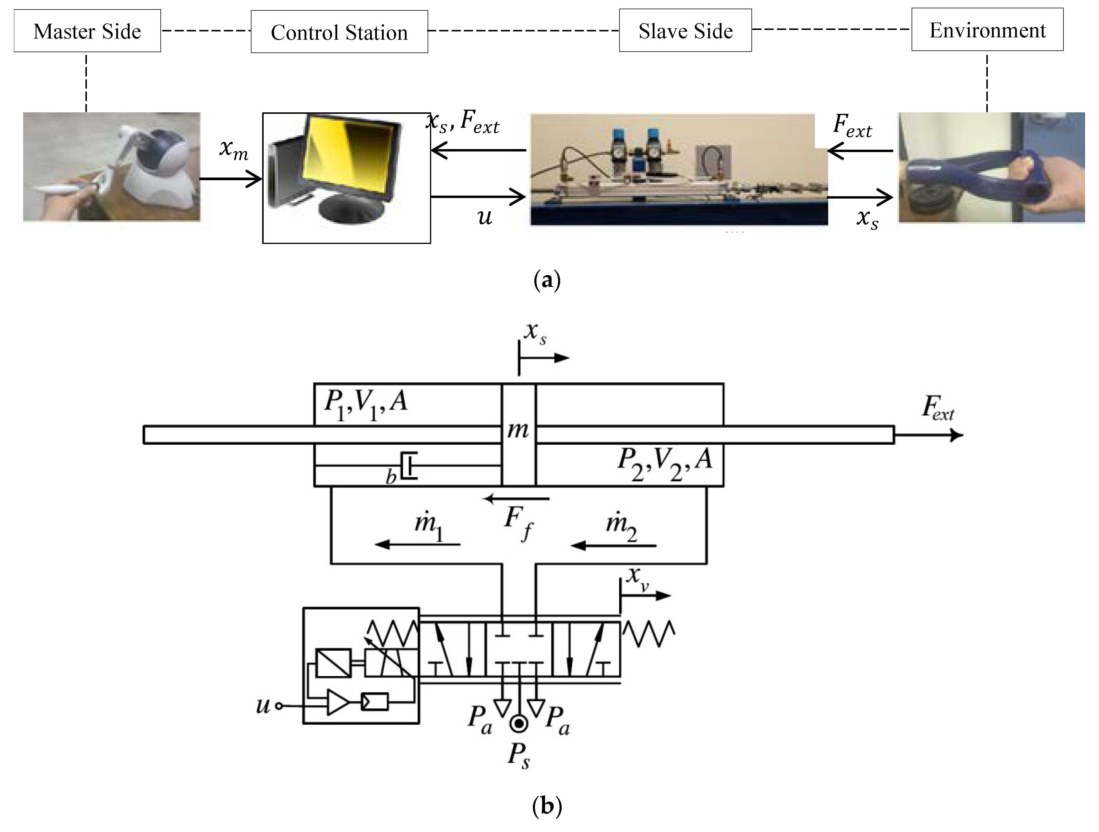
2. Experimental Setup

Figure 1 shows the experimental setup of the system under study. A PHANTOM joystick is used as the master manipulator. It is capable of serial communication using a high speed IEEE1394 communication protocol (FireWire), which is available on many computers. The slave manipulator is a single degree-of-freedom pneumatic actuator, which interacts with the environment (a human subject) through a handle. A computer with Quanser data acquisition board facilitates the connection of the master and the slave through a local network with negligible delay.
The pneumatic setup, shown in Figure 1b, is a double rod (FESTO DNC) with 500 mm stroke. The bore and rod diameter are 40 mm and 16 mm respectively. A proportional directional flow control valve (FESTO MPYE) sends the pressurized air to the cylinder to move it according to the movement of the master. The maximum flow capacity of the control valve is 700 L/min at 7 bar (100 psi) absolute supply pressure. The master, force sensor (ARTECH S type load cell), position encoder (BOURNS incremental rotary encoder) and pressure sensors (by Durham Industries) also send data to the control station. The above components are connected to a local network, which is assumed ideal, meaning the network characteristics such as time delay and packet loss are negligible. The sampling frequency is 500 Hz.
Referring to Figure 1b, the equation of motion of the actuator is defined as:
m x ¨ s = A ( P 1 P 2 ) + F e x t ( F f +   b x ˙ s )
where m is the mass of the moving parts, x s is the actuator position, P 1 and P 2 are the air pressures at of the actuator chambers, and A represents the piston area. b is the viscous friction coefficient and F e x t is the externally applied load. The dry friction, F f , is adopted from LuGre friction model [22] without its viscous friction term as viscous friction is already included as a separate term in (1):
F f = σ 0 z + σ 1 z ˙
where σ 0 is the equivalent spring constant and σ 1 is the damping coefficient of bristles. The variable z , average bristle deflection, can be achieved by solving the following equation [22]:
z ˙ = x ˙ s σ 0 | x ˙ s | z F c + ( F s F c ) e ( x ˙ s / v s v ) 2
where F c and F s are the Coulomb friction and static friction, respectively, and v s v is the Stribeck velocity. To move the actuator, air pressure should be charged or discharged into chambers. The air pressure is related to the air mass flows, m ˙ 1 and m ˙ 2 , as follows [21,23]:
P ˙ 1 = γ R T m ˙ 1 V 1 α γ A x ˙ s P 1 V 1
P ˙ 2 = γ R T m ˙ 2 V 2 + α γ A x ˙ s P 2 V 2
V 1 = V 0 + A x s
V 2 = V 0 + A ( L x s )
In (4) and (5), R is the ideal gas constant, γ is the ratio of specific heats, α is compressibility correction factor and T is air temperature [24]. V 1 and V 2 are the volumes of each actuator chambers, which are functions of the actuator position as expressed in (6) and (7). L is the length of the actuator stroke and V 0 presents cylinder inactive volume. By defining γ ¯ = γ ( 2 / ( γ + 1 ) ) ( γ + 1 ) / ( γ 1 ) / R , the mass flow rate of air through control valve orifice can be expressed as [25]:
{ m ˙ 1 = w x v   ˙ 1 = { w x v   C d P s T γ ¯ , P 1 P s P c r w x v   C d P s T γ ¯ 1 ( P 1 / P s P c r 1 P c r ) ( γ 1 ) / γ , P 1 P s > P c r m ˙ 2 = w x v ˙ 2 = { w x v   C d P 2 T γ ¯ , P a P 2 P c r w x v   C d P 2 T γ ¯ 1 ( P a / P 2 P c r 1 P c r ) ( γ 1 ) / γ , P a P 2 > P c r }   x v 0 m ˙ 1 = w x v   ˙ 1 = { w x v   C d P 1 T γ ¯ , P a P 1 P c r w x v   C d P 1 T γ ¯ 1 ( P a / P 1 P c r 1 P c r ) ( γ 1 ) / γ , P a P 1 > P c r m ˙ 2 = w x v ˙ 2 = { w x v   C d P s T γ ¯ , P 2 P s P c r w x v   C d P s T γ ¯ 1 ( P 2 / P s P c r 1 P c r ) ( γ 1 ) / γ , P 2 P s > P c r } x v < 0
where w and ˙ i   ( i = 1 , 2 ) are orifice area gradient and mass flow per area unit, respectively. x v represents the displacement of the valve spool, C d is discharge coefficient of the valve, P c r is the valve critical pressure ratio, and P a and P s are the absolute downstream and upstream pressures, respectively. The valve orifice area gradient, w , is related to the control signal by the following equation:
x ˙ v = 1 τ ( x v + K v u )
where u is the control signal, K v is the valve spool position gain and τ is the valve time constant. The values of the parameters of the test rig are shown in Table 1 that are either provided by the manufacturers or obtained experimentally through previous research [26].

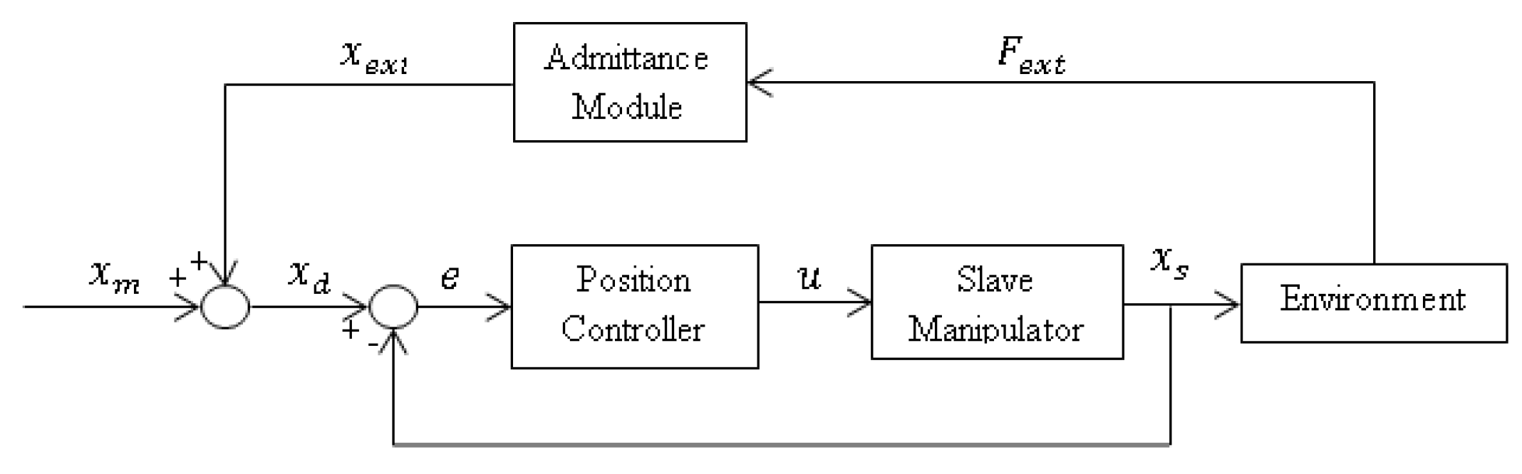
3. Control Architecture

3.1. Admittance Control

Admittance control simultaneously maintains the desired force and position in the same direction [13,27]. It provides the system with a function which converts the external force, F e x t , to a corresponding position called external position, x e x t . Figure 2 shows the general block diagram of admittance control where x e x t is added to the primary desired position, x m , determined by the master manipulator. In this approach, the position controller tracks a modified desired trajectory, x d , that is the combination of the primary desired trajectory, x m , and the displacement correspondent to the external force, x e x t ( x d =   x m + x e x t ). The relationship between the external force, F e x t , and the corresponding displacement, x e x t , is usually defined by a second-order linear mass-spring-damper model as follows:
x e x t F e x t = 1 M s 2 + B s + K
where M , B and K are admittance parameters corresponding to inertia, damping and stiffness characteristics and s is the Laplace operator. Response of the manipulator to the external force can be tuned by tuning admittance parameters.

3.2. Position Controller

To position the pneumatic actuator, Sliding Mode Control (SMC) scheme is employed. SMC is a model-based scheme that provides a robust performance despite model uncertainties [21,28,29]. It is the most popular position controller for pneumatic actuators [7,29]. In order to design an SMC algorithm, an integral sliding surface is defined as:
S = ( d d t + δ ) 3 0 t e   d τ
where δ is a positive constant and e is the position error, defined as follows:
e = x s x d = x s ( x m + x e x t )
The SMC control law is obtained by summing up an equivalent control component formulated based on the dynamic model, A v e q , with a robustness control component, A v r b :
u = ( A v e q + A v r b ) / ( w K v )
where K v is the valve spool position gain and w is the valve orifice area. Dynamics of the system on the sliding surface can be expressed as [15]:
S ˙ = e + δ 3 e + 3 δ 2 e ˙ + 3 δ e ¨ = 0
By replacing e with x s x d and then obtaining x s from (14) and applying it to (1), the following expression for the equivalent component is achieved:
A v e q = x d δ 3 e 3 δ 2 e ˙ 3 δ e ¨ F x P x
In (15), P x and F x are derived as:
P x = γ R T A m ( ˙ 1 V 1 + ˙ 2 V 2 )
F x = K x ˙ s F ˙ e x t + b x ¨ s + F ˙ f m
where
K = α γ A 2 ( P 1 V 1 + P 2 V 2 )
Considering the slow dynamics of the system, the rate of changes in dry friction, F f , is slow. Thus, F ˙ f in (17) can be neglected. Same assumption was made in previous studies [7,28,29]. The role of the robust part of SMC, A v r b , is to provide robustness despite this assumption. A v r b is formulated as follows:
A v r b = K r b P x s i g n   ( S )
where K r b is a positive gain. Because the discontinuouty of sign function in (19) is not ideal for practical implementation, it is approximated by the continuous tanh function as follows:
s i g n ( S )   t a n h ( a S )
where a is a large positive number.

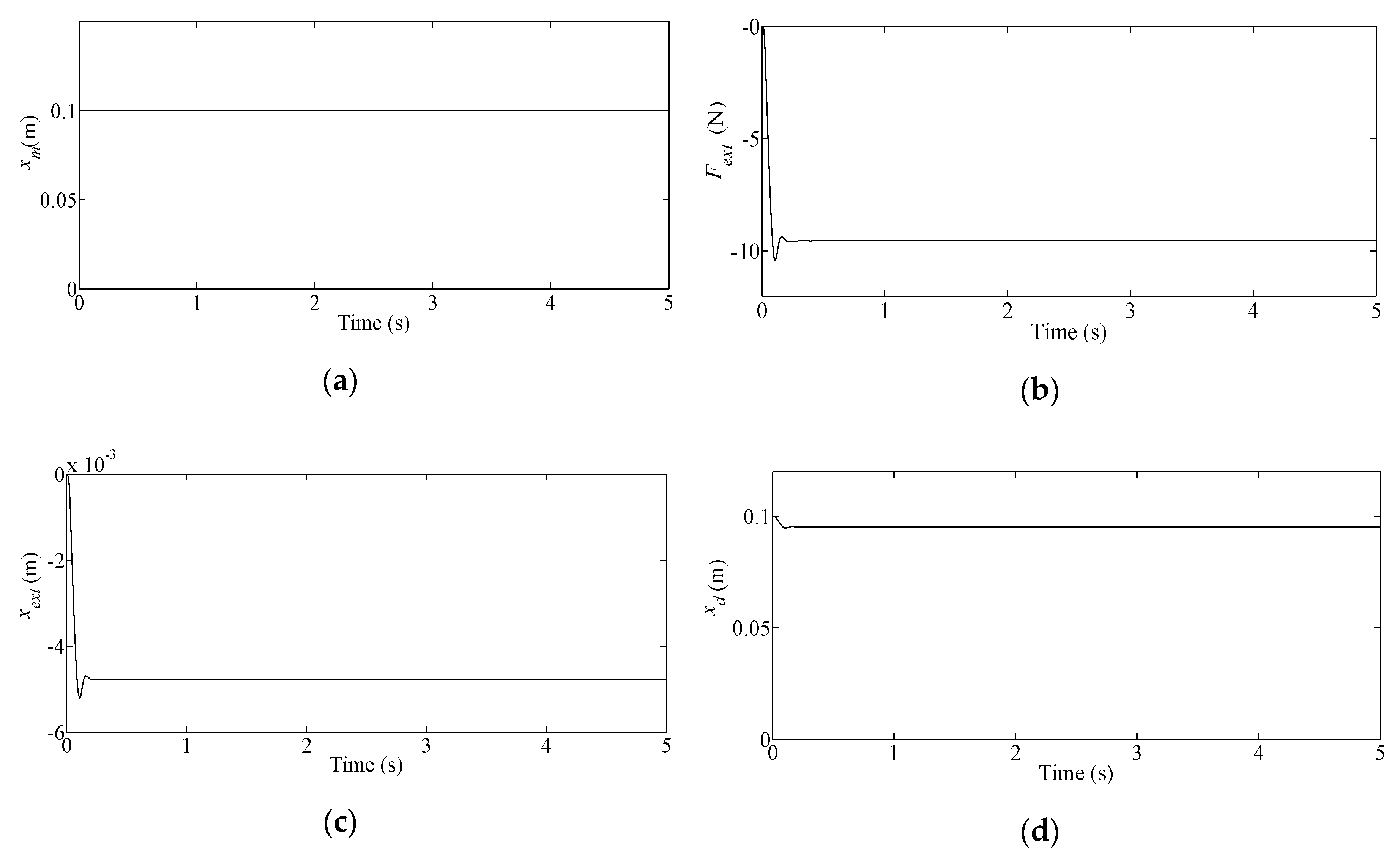
4. Simulation Studies

The performance of the proposed unilateral pneumatic system is first evaluated through simulations. Referring to Figure 1, the teleoperated control system receives the displacement of the master, x m , and the external force imparted to the slave from the environment, F e x t . The environment is considered spring-dominant which means F e x t is proportional to the slave position:
F e x t = K e x t x s
where K e x t is the stiffness coefficient of the environment.
A simplified admittance model is employed whereby the external force is related to the external position by a virtual spring:
x e x t = F e x t / K a d m
In (22), K a d m is a positive coefficient corresponding to the stiffness term in the admittance model. The step tracking simulation results for the admittance control are shown in Figure 3. The system step input, x m , is 0.1 m as shown in Figure 3a. Considering K e x t = 100   N / m , the external force, F e x t , is shown in Figure 3b. The external position, x e x t , is derived from (22), considering K a d m = 2000   N / m , and shown in Figure 3c. The modified desired trajectory, x d , is obtained by adding the primary desired trajectory, x m , and the external position, x e x t and shown in Figure 3d.
Figure 4 shows the corresponding slave manipulator variables. The controller parameters are δ = 80   rad / s and K r b = 2000   m / s 3 . The numerical value of a in (20) is chosen as 10 4 . The slave position, x s , is shown in Figure 4a. The air pressures in cylinder chambers are shown in Figure 4b. The control signal applied to the slave actuator is shown in Figure 4c and does not saturate. The control signal of this system changes within the range of 0–10 V. Hence, with the 5 V control signal, the valve is fully closed. The position tracking error, defined by (12), is shown in Figure 4d. It is seen that there is a reasonable agreement between motions of slave and master actuators.

5. Stability Analysis

The concept of Lyapunov exponents (LEs) is a well-established numerical approach to study nonlinear systems [9,20]. LEs indicate stability of a nonlinear system by monitoring the long-term behaviour of adjacent state-space trajectories as time evolves. The total number of LEs is equal to the dimension of the state space and the sign of the LEs is used to deduce the stability property of the system. A positive LE corresponds to chaotic or unstable behavior. When all of the exponents are negative, all of the neighboring trajectories converge as time evolves indicating that the system is exponentially stable with a fixed equilibrium point. If there is one zero exponent and the other exponents are negative, we have a stable system with one-dimensional equilibrium [30]. Presenting the required conditions for employing the Lyapunov exponent method is avoided to keep the focus of the paper. More details can be found in [23].

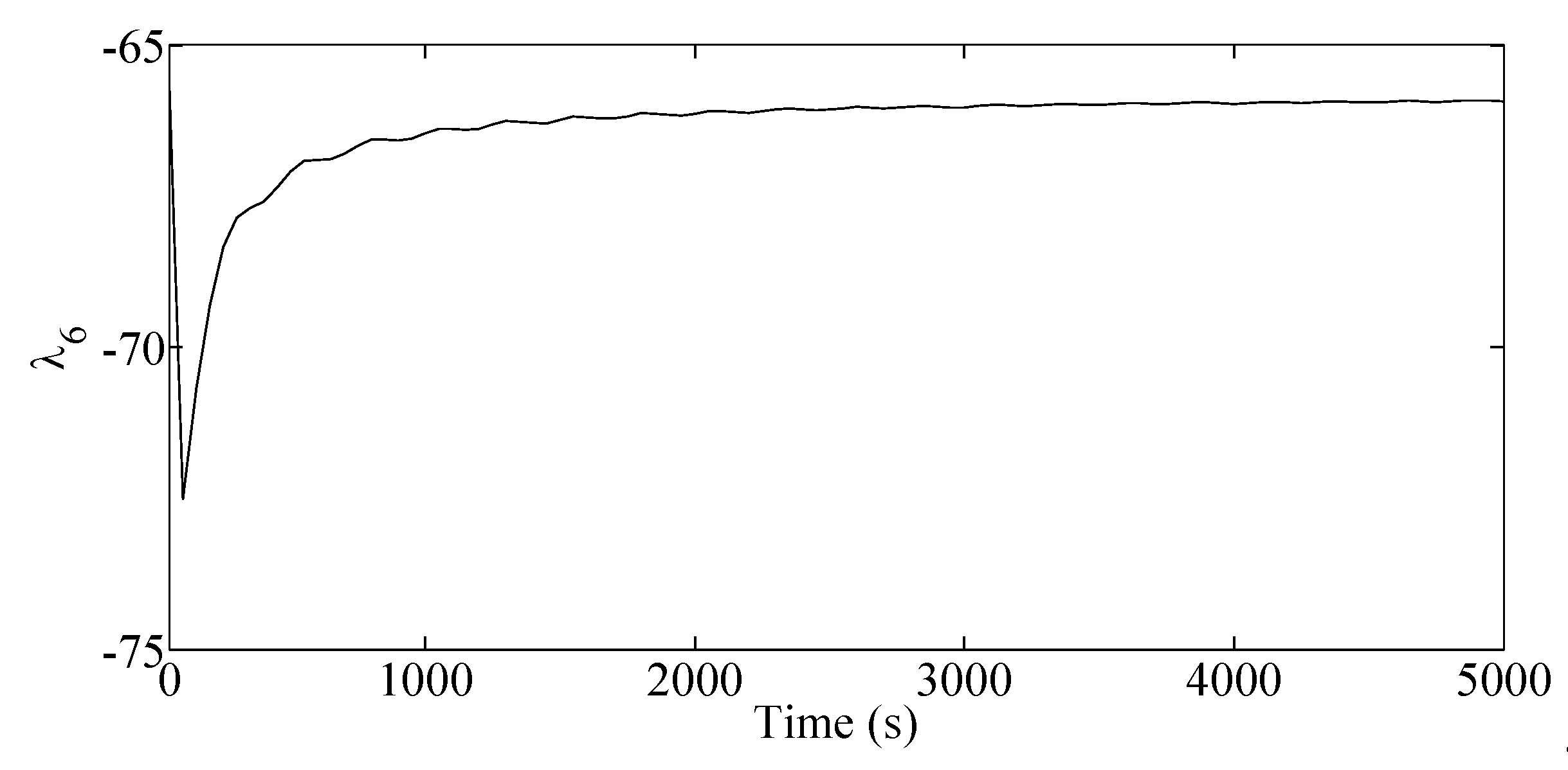
5.1. Calculation of Lyapunov Exponents

Consider the following smooth nonlinear system in an n-dimensional state space:
x ˙ = f ( x )
where x R n , is the state vector and f ( x ) is continuous and differentiable. To calculate LEs, a “fiducial” trajectory is found by solving (23) using initial condition x ( 0 ) = x 0 . Orthogonal principal axes, δ x , are then defined on the fiducial trajectory. The asymptotic behaviour of the nonlinear system could be determined by monitoring the length of each principal axis over time. To find the length of the i-th ( i = 1 ,   , n ) principal axis, a linear equation of motion is formed as:
ψ ˙ t = F ( t ) ψ t
where F ( t ) is the Jacobian matrix:
F ( t ) = f x T |   x = x ( t )
Each principal axis is a column of ψ t . Since the resulting principal axes tend to fall along the direction of the fastest growing axis, Gram-Schmidt reorthonormalization scheme is applied to make the axes orthogonal to each other and then normalize their lengths in every iteration [31]. The i-th LE is obtained using the following key equation [31]:
λ i = l i m t 1 T l n   δ x i ( t ) δ x i ( t 0 )
where T is the total duration of the observance. [23] details a simple example of calculating LEs.

5.2. Stability Analysis of the Proposed Control System

The stability analysis of the entire control system described in Section 3 is conducted. The state space model is formed by defining the state space vector as:
x = [ x 1   x 2   x 3   x 4   x 5   x 6   x 7 ] T = [ x s   v s   P 1   P 2   x v   z   0 t e   d τ ] T
where x s and v s are displacement and the velocity of the piston, P 1 and P 2 are air pressures in each actuator chamber, x v is the displacement of spool valve as a result of the control signal, z is average bristle deflection and 0 t e   d τ is the integral of the position error as defined by (12). Using the state variables, (27), and Equations (1)–(9), (21) and (22), the state space model is constructed as
{ x ˙ 1 = x 2 x ˙ 2 = 1 m [ A ( x 3 x 4 ) K e x t x 1 b x 2 ( σ 0 x 6 + σ 1 ( x 2 ( σ 0 | x 2 | x 6 / F c + ( F s F c ) e ( x 2 / v s ) 2 ) ) ) ] x ˙ 3 = γ R T ( w x 5   ˙ 1 / ( V 0 + A x 1 ) ) α γ A ( x 2 x 3 / ( V 0 + A x 1 ) ) x ˙ 4 = γ R T ( w x 5   ˙ 2 / ( V 0 + A ( L x 1 ) ) ) + α γ A ( x 2 x 4 / ( V 0 + A ( L x 1 ) ) x ˙ 5 = ( x 5 + K v u ) / τ x ˙ 6 = x 2 ( σ 0 | x 2 | x 6 / F c + ( F s F c ) e ( x 2 / v s ) 2 ) x ˙ 7 = e
The control signal in terms of state space variables is obtained by substituting (15) and (19) into (13):
u = 1 w K v ( x d δ 3 e 3 δ 2 e ˙ 3 δ e ¨ F x K r b   t a n h ( S ) γ R T A m ( ˙ 1 V 0 + A x 1 + ˙ 2 V 0 + A ( L x 1 ) ) )
The associated variables in (29) are defined as:
x d = K e x t K a d m m ( A ( x ˙ 3 x ˙ 4 ) b m ( A ( x 3 x 4 ) K e x t x 1 b x 2 F f ) K e x t x 2 )  
F x = α γ A 2 m ( x 3 V 0 + A x 1 + x 4 V 0 + A ( L x 1 ) ) x 2 K e x t m x 2 b m 2 ( A ( x 3 x 4 ) K e x t x 1 b x 2 F f )
S = δ 3 x 7 + 3 δ 2 e + 3 δ e ˙ + e ¨    
e = ( 1 + K e x t K a d m ) x 1 x m
e ˙ = ( 1 + K e x t K a d m ) x 2
e ¨ = 1 m ( 1 + K e x t K a d m ) x ˙ 2
The dry friction in the state space is as follows:
F f = σ 0 x 6 + σ 1 x 2 σ 0 σ 1 | x 2 | x 6 F c + ( F s F c ) e ( x 2 / v s v ) 2
The mass flow rate per area unit in state space is defined as:
{ ˙ 1 = { C d P s T γ ¯ , x 3 P s P c r C d P s T γ ¯ 1 ( x 3 / P s P c r 1 P c r ) ( γ 1 ) / γ , x 3 P s > P c r ˙ 2 = { C d x 4 T γ ¯ , P a x 4 P c r C d x 4 T γ ¯ 1 ( P a / x 4 P c r 1 P c r ) ( γ 1 ) / γ , P a x 4 > P c r   x 5 0   ˙ 1 = { C d x 3 T γ ¯ , P a x 3 P c r C d x 3 T γ ¯ 1 ( P a / x 3 P c r 1 P c r ) ( γ 1 ) / γ , P a x 3 > P c r ˙ 2 = { C d P s T γ ¯ , x 4 P s P c r C d P s T γ ¯ 1 ( x 4 / P s P c r 1 P c r ) ( γ 1 ) / γ , x 4 P s > P c r x 5 < 0
The equilibrium point of (28) is:
x e q = [ x m 1 + K e x t K a d m ,   0 ,   x 3 s s ,   x 4 s s ,   0 ,   x 6 s s ,   0 ] T
where
A ( x 3 s s     x 4 s s ) K e x t x m 1 + K e x t K a d m σ 0 x 6 s s = 0
To study the stability of the control system, the LEs are calculated and summarized in Table 2. Note that theoretically, Lyapunov exponents are defined when t . In practice however, we calculate them over limited time duration and the adequate calculation time can be determined by observing the exponents variation over time. As an example, time evolution of λ 6 is shown in Figure 5.
The signs of Lyapunov exponents determine the stability property of the dynamic system. Negative exponents correspond to exponential stability. The first largest exponent being zero indicates stable system with one-dimensional attractor. To understand the physical meaning of the results in Table 2, (38) and (39) are revisited. According to these equations, x 1 s s , x 2 s s and x 5 s s will eventually reach fixed values where the combination of x 3 s s , x 4 s s and x 6 s s will not hold fixed points but satisfy (39). Having three unknowns ( x 3 s s , x 4 s s , x 6 s s ) and one equation, (39) will have a 2-dimentional solution; i.e., the equilibrium of (28) is 2-dimentional. This explains the two zero LEs in Table 2. Therefore, the stability of the proposed control system in presence of external force and model uncertainties is proven, as seen in Table 2.

5.3. Parametric Stability Analysis

Parametric stability analysis is the stability analysis of a dynamic system as its parameters change. It is beneficial when some parameters of the system are unknown, inaccurate or varying. The concept of Lyapunov exponents can be used for this reason. Because it provides a quantitative measurement of the stability, one can find the stability region of a system by changing the values of the physical parameters of the system or the controller gains [30]. Not only the concept of LEs can assure the stability of a system when the parameters are varying, it can be used to measure the effect of changing parameters on overall stability.
Parametric stability analysis of the teleoperation system under investigation is conducted using the concept of LEs. The stiffness coefficient of the environment denoted by K e x t , and controller gain, δ , were considered for this purpose. Table 3 shows the numerical values of LEs for admittance unilateral teleoperation as K e x t varies. It is evident that changing K e x t does not change the values of LEs notably. Table 4 shows the numerical values of LEs while the SMC bandwidth gain, δ , varies. The system is stable for the values of δ 120 . However, for δ = 140 , the first LE is positive which denote that the system is chaotic.

6. Experimental Results

Experiments were performed to evaluate the performance of the teleoperated pneumatic system under real test scenarios. Different admittance parameter settings were tested. Two experimental scenarios are presented to show the performance of the admittance control in conjunction with SMC. In the first experiment, the admittance parameters are set to study soft reaction to an external force. In the second experiment, an external force is applied to the actuator and the goal of the admittance model is a stiff actuator reaction.
Experiment 1: In this experiment, the operator moves the master and, at the same time, a human subject located at the slave side applies a force to the pneumatic actuator. The external force passes through the admittance model (10), having parameters set as M = 10   Kg , B = 50   Ns / m and K = 250   N / m . The desired position trajectory originating from the master, x m , is shown in Figure 6a. Figure 6b shows the external force. The modified desired trajectory is shown in Figure 6c. It is evident that the admittance control module effectively adjusts the primary desired trajectory according to the imposed external force. This figure also compares the modified desired trajectory with the actual position of the actuator and illustrates their reasonable agreement. Figure 6d shows the control signal, which is also reasonable and unsaturated. This experiment shows successful application of admittance control with soft stiffness.
Experiment 2: In this experiment, the parameters of the admittance model are set to M = 10   Kg , B = 50   Ns / m and K = 10 4   N / m . The goal is to study the behaviour of the system when the stiffness of admittance model is set high. The actuator is subject to an external force with the magnitude of 100 N applied by a human subject. As Figure 7a shows, the primary desired position is fixed during the experiment. The external force is shown in Figure 7b. The admittance model in (10) converts the external force to small displacement as shown in Figure 7c. For external force with 100 N magnitude, the change in primary desired trajectory is about 0.01 m. By comparing Figure 7c and Figure 6c, the effect of changes in the parameters of the admittance control module can be studied. Figure 7c also shows the actual position of slave actuator, x s . Figure 7d shows the control signal corresponding to the position tracking shown in Figure 7c.
The above experiments show the proposed unilateral control system can successfully control the slave actuator desired position in the presence of the external force. The stability of the actuator motion was evident in the experiments. The SMC position controller worked effectively despite the non-idealities such as friction and air compressibility.
The positioning accuracy of the admittance method presented in this paper is now compared with the accuracy of the impedance method, previously developed by the authors on the same system. The comparison is done by calculating the average position error for the same experiments. The results are summarized in Table 5:
According to Table 5, admittance unilateral teleoperation provides higher tracking accuracy. This is expected since admittance unilateral teleoperation utilizes an SMC position controller. Whereas, in impedance unilateral, an SMC force controller is in charge of tracking the position.

7. Conclusions

In this paper, a unilateral teleoperation system was analyzed, and successfully implemented on a pneumatic actuator. Admittance control, coupled with a sliding mode position controller, was employed to manage actuator position and external force in the slave side. The proposed control system not only inherited the structural advantages of the unilateral teleoperation system with no need for highly skilled operator, but also displayed satisfactory performance in scenarios involving various levels of environmental stiffness and interactions. Both simulation and experimental results showed the effectiveness of the proposed unilateral teleoperation system in position tracking and handling the external force. Meanwhile, stability of the entire control system was evaluated using the concept of Lyapunov exponents. Parametric stability analysis showed the system remains stable for a wide range of the environmental stiffnesses whereas increasing the controller gain leads to system instability. Future work can focus on extension of the controller presented here to multi-degree of freedom pneumatic manipulators, and the stability analysis of the entire system.

Author Contributions

Conceptualization, N.G. and N.S.; methodology, N.G., Y.S., P.S. and C.X.Y.; software, N.G., Y.S. and C.X.Y.; validation and analysis, N.G. and N.S.; resources, P.S., C.X.Y. and Y.S.; writing—original draft preparation, N.G.; writing—review and editing, Y.S., P.S. and N.S.; supervision, N.S.; project administration, N.S.; funding acquisition, N.S. All authors have read and agreed to the published version of the manuscript.

Funding

This research was funded by NSERC (Natural Sciences and Engineering Research Council) of Canada; Grant number: RGPIN-2018-05352.

Acknowledgments

This work was supported by the Natural Sciences and Engineering Research Council (NSERC) of Canada.

Conflicts of Interest

The authors declare no conflict of interest.

References

  1. Lawrence, P.; Salcudean, S.; Sepehri, N.; Chan, D.; Bachmann, S.; Parker, N.; Zhu, M.; Frenette, R. Coordinated and Force Feedback Control of Hydraulic Excavators. In Proceedings of the 4th International Symposium of Experimental Robotics, Stanford, CA, USA, 30 June–2 July 1995. [Google Scholar]
  2. Kontz, M.; Beckwith, J.; Book, W. Evaluation of a teleoperated haptic forklift. In Proceedings of the IEEE/ASME International Conference on Advanced Intelligent Mechatronics, Monterey, CA, USA, 24–28 July 2005. [Google Scholar]
  3. Hokayem, P.F.; Spong, M.W. Bilateral teleoperation: An historical survey. Automatica 2006, 42, 2035–2057. [Google Scholar] [CrossRef]
  4. Le, M.; Pham, M.; Tavakoli, M.; Moreau, R. Sliding Mode Control of a Pneumatic Haptic Teleoperation System with on/off Solenoid Valves. In Proceedings of the IEEE International Conference on Robotics and Automation, Anchorage, AK, USA, 3–7 May 2010. [Google Scholar]
  5. Tadano, K.; Kawashima, K. Development of a Master–Slave System with Force-Sensing Abilities using Pneumatic Actuators for Laparoscopic Surgery. J. Adv. Robot. 2010, 24, 1763–1783. [Google Scholar] [CrossRef]
  6. Anderson, R.J. Bilateral control of teleoperators with time delay. IEEE Trans. Autom. Control 1989, 34, 494–501. [Google Scholar] [CrossRef]
  7. Dakkan, K.; Barth, E.; Goldfarb, M. Dynamic constraint based energy saving control of pneumatic servo systems. ASME J. Dyn. Syst. Meas. Control 2006, 128, 655–662. [Google Scholar] [CrossRef]
  8. Zarei-nia, K.; Sepehri, N. Lyapunov stable displacement-mode haptic manipulation of hydraulic actuators: Theory and experiment. Int. J. Control 2012, 85, 1313–1326. [Google Scholar] [CrossRef]
  9. Yang, C.; Wu, Q.; Zhang, P. Estimation of Lyapunov exponents from a time series for N-dimensional state space using nonlinear mapping. Nonlinear Dyn. 2012, 69, 1493–1507. [Google Scholar] [CrossRef]
  10. Hannaford, B. A design framework for teleoperators with kinesthetic feedback. IEEE Trans. Robot. Autom. 1989, 5, 426–434. [Google Scholar] [CrossRef] [Green Version]
  11. Leleve, A.; Pham, M.; Tavakoli, M.; Moreau, R. Towards Delayed Teleoperation with Pneumatic Master and Slave for MRI. In Proceedings of the ASME Biennial Conference on Engineering Systems Design and Analysis, Nantes, France, 2 July 2012. [Google Scholar]
  12. Hodgson, S.; Le, M.; Tavakoli, M.; Pham, M. Improved tracking and switching performance of an electro-pneumatic positioning system. J. Mechatron. 2012, 22, 1–12. [Google Scholar] [CrossRef] [Green Version]
  13. Hogan, N.; Buerger, S. Impedance and Interaction Control. In Robotics and Automation Handbook; CRC Press: Boca Raton, FL, USA, 2004; Chapter 19; p. 24. [Google Scholar]
  14. Durbha, V.; Li, P. Passive Bilateral Teleoperation and Human Power Amplification with Pneumatic Actuators. In Proceedings of the ASME Dynamic Systems and Control Conference, Hollywood, CA, USA, 12–14 October 2009. [Google Scholar]
  15. Khalil, H. Nonlinear Systems; Prentice Hall: Upper Saddle River, NJ, USA, 1995. [Google Scholar]
  16. Hogan, N. Controlling impedance at the man/machine interface. In Proceedings of the IEEE International Conference on Robotics and Automation, Scottsdale, AZ, USA, 14–19 May 1989. [Google Scholar]
  17. Durbha, V.; Li, P. Passive Tele-Operation of Pneumatic Powered Robotic Rescue Crawler. In Proceedings of the 6th FPNI-PhD Symposium, West Lafayette, IN, USA, 15–19 June 2010. [Google Scholar]
  18. Li, H.; Tadano, K.; Kawashima, K. Achieving Force Perception in Master-Slave Manipulators Using Pneumatic Artificial Muscles. In Proceedings of the Society of Instrument & Control Engineers (SICE) Annual Conference, Akita, Japan, 20–23 August 2012. [Google Scholar]
  19. Hogan, N. Impedance control: An approach to manipulation part I,II,III. J. Dyn. Syst. Meas. Control 1985, 107, 1–24. [Google Scholar] [CrossRef]
  20. Sekhavat, P.; Sepehri, N.; Wu, C. Overall Stability Analysis of Hydraulic Actuator’s Switching Contact Control Using the Concept of Lyapunov Exponents. In Proceedings of the International Conference on Robotics and Automation, Barcelona, Spain, 18–22 April 2005. [Google Scholar]
  21. Garmsiri, N.; Sun, Y.; Yang, C.; Sepehri, N. Bilateral teleoperation of a pneumatic actuator: Experiment and stability analysis. Int. J. Fluid Power 2015, 16, 99–110. [Google Scholar] [CrossRef]
  22. De Wit, C.C.; Olsson, H.; Astrom, K.; Lischinsky, P. A new model for control of systems with friction. IEEE Trans. Autom. Control 1995, 40, 419–425. [Google Scholar] [CrossRef] [Green Version]
  23. Liu, S.; Bobrow, J. An analysis of a pneumatic servo system. Trans. ASME J. Dyn. Syst. Meas. Control 1988, 110, 228–235. [Google Scholar] [CrossRef]
  24. Richer, E.; Hurmuzlu, Y. A High Performance Pneumatic Force Actuator System: Part II—Nonlinear Controller Design. J. Dyn. Syst. Meas. Control 2000, 122, 426–434. [Google Scholar] [CrossRef]
  25. Sanville, F. A new method of specifying the flow capacity of pneumatic fluid power valves. BHRA 2nd Int. Fluid Power Symp. 1971, D337–D347. [Google Scholar]
  26. Karpenko, M.; Sepehri, N. Development and Experimental Evaluation of a Fixed-Gain Nonlinear Control for a Low-Cost Pneumatic Actuator. IEEE Proc. Control Theory Appl. 2006, 153, 629–640. [Google Scholar] [CrossRef]
  27. Richardson, R.; Brown, M.; Bhakta, B.; Levesley, M. Impedance control for a pneumatic robot-based around pole-placement, joint space controllers. J. Control Eng. Pract. 2005, 13, 291–303. [Google Scholar] [CrossRef]
  28. Shen, X. Nonlinear model-based control of pneumatic artificial muscle servo systems. J. Control Eng. Pract. 2010, 18, 311–317. [Google Scholar] [CrossRef]
  29. Gulati, N.; Barth, E. A Globally Stable, Load-Independent Pressure Observer for the Servo Control of Pneumatic Actuators. IEEE ASME Trans. Mechatron. 2009, 14, 295–306. [Google Scholar] [CrossRef]
  30. Sadri, S.; Wu, C. Stability analysis of a nonlinear vehicle model in plane motion using the concept of Lyapunov exponents. Int. J. Veh. Mech. Mobil. 2013, 51, 906–924. [Google Scholar] [CrossRef]
  31. Wolf, A.; Swift, J.; Swinney, H.; Vastano, J. Determining Lyapunov Exponents from a Time Series. J. Phys. 1985, 16, 285–317. [Google Scholar] [CrossRef] [Green Version]
  32. Garmsiri, N.; Sun, Y.; Sepehri, N. Impedance Control of a Teleoperated Pneumatic Actuator: Implementation and Stability Analysis. ACTA Control Intell. Syst. 2017, 45, 19–30. [Google Scholar]
Publisher’s Note: MDPI stays neutral with regard to jurisdictional claims in published maps and institutional affiliations.
Figure 1. (a) Test setup of unilateral admittance-controlled of the pneumatic actuator; (b) schematic diagram of pneumatic system [21].
Actuators 09 00103 g001
Figure 2. General block diagram of admittance control.
Actuators 09 00103 g002
Figure 3. Admittance control variables pertaining to step tracking: (a) primary desired trajectory provided by the master manipulator, x m ; (b) external force, F e x t ; (c) displacement corresponding to the external force, x e x t ; (d) desired trajectory achieved from admittance model, x d .
Actuators 09 00103 g003
Figure 4. Step tracking with SMC: (a) piston position; (b) chamber pressures; (c) control signal; (d) position error.
Actuators 09 00103 g004
Figure 5. Time evolution of λ 6 .
Actuators 09 00103 g005
Figure 6. Experimental study of low Stiffness admittance model while tracking a human-guided trajectory: (a) primary desired position by master manipulator, x m ; (b) external force, F e x t ; (c) modified desired trajectory, x d , versus position of actuator, x s ; (d) control signal, u .
Actuators 09 00103 g006
Figure 7. Experimental study of high stiffness admittance model while tracking a human-guided trajectory: (a) primary desired position by the master manipulator, x m ; (b) external force, F e x t ; (c) modified desired trajectory, x d , versus position of actuator, x s ; (d) control signal, u .
Actuators 09 00103 g007
Table 1. Parameters of Pneumatic Actuator [26].
ParameterSymbol (Unit)Value
Actuator stroke L   ( m ) 0.5
Piston annulus area A ( cm 2 ) 10.6
Valve time constant τ   ( ms ) 4.2
Valve orifice area gradient w   ( mm 2 / mm ) 22.6
Supply pressure P s ( bar )5
Valve coefficient of discharge C d 0.7
Static friction F s   ( N ) 38.5
Coulomb friction F c   ( N ) 32.9
Ratio of specific heats γ 1.4
Ideal gas constant R   ( J / kgK ) 287
Valve critical pressure ratio P c r 0.2
Valve spool gain K v   ( mm / V ) 0.25
Damping coefficient of bristle σ 1 ( N / m / s ) 93.13
Spring constant of bristle σ 0   ( N / m ) 4500
Mass of moving parts m ( kg ) 1.91
Compressibility correction factor α 1.2
Temperature of air T   ( K ) 300
Atmospheric pressure P a   ( bar ) 1
Viscous damping coefficientb (Ns/m)70
Stribeck velocity v s v   ( m / s ) 0.02
Cylinder inactive volume V 0   ( m 3 ) 1.64 × 10 4
Table 2. Values of Lyapunov Exponents for Step Tracking Task.
λ 1 λ 2 λ 3 λ 4 λ 5
0.00.0−0.1−17.8−18.0
Table 3. Numerical results of LEs for admittance unilateral teleoperation as K e x t varies.
K e x t   ( N / m ) λ 1 λ 2 λ 3 λ 4 λ 5 λ 6 λ 7
100.00.0−0.1−17.7−18.0−75.7−229.3
500.00.0−0.1−17.8−18.0−75.7−229.3
1000.00.0−0.1−17.8−18.0−75.5−229.4
1500.00.0−0.1−17.8−18.1−75.5−229.5
2000.00.0−0.1−17.9−18.1−75.4−229.6
3000.00.0−0.1−17.9−18.1−75.3−229.7
6000.00.0−0.1−18.1−18.6−74.8−230.1
Table 4. Numerical results of LEs for admittance unilateral teleoperation as δ varies.
δ   ( r a d / s ) λ 1 λ 2 λ 3 λ 4 λ 5 λ 6 λ 7
200.00.0−0.1−19.8−64.6−64.7−191.4
300.00.0−0.1−26.0−56.1−56.1−202.3
400.00.0−0.1−34.3−47.8−47.8−210.7
600.00.0−0.1−31.7−31.9−55.0−222.2
800.00.0−0.1−17.8−18.1−75.5−229.4
1000.00.0−0.4−13.2−14.5−83.2−230.0
1200.00.0−0.7−7.5−34.4−70.9−228.0
14056.6------
Table 5. Comparison of the position errors.
MethodAvg. Position Error (mm)Refer to
Admittance Unilateral1.3Figure 6 and Figure 7
Impedance Unilateral [32]9.1Figures 6–8 of Reference [32]

