Optimal Force Allocation and Position Control of Hybrid Pneumatic–Electric Linear Actuators

Abstract

Hybrid pneumatic–electric actuators (HPEAs) are redundant actuators that combine the large force, low bandwidth characteristics of pneumatic actuators with the large bandwidth, small force characteristics of electric actuators. It has been shown that HPEAs can provide both accurate position control and high inherent safety, due to their low mechanical impedance, making them a suitable choice for driving the joints of assistive, collaborative, and service robots. If these characteristics are mathematically modeled, input allocation techniques can improve the HPEA’s performance by distributing the required input (force or torque) between the redundant actuators in accordance with each actuator’s advantages and limitations. In this paper, after developing a model for a HPEA-driven system, three novel model-predictive control (MPC) approaches are designed that solve the position tracking and input allocation problem using convex optimization. MPC is utilized since the input allocation can be embedded within the motion controller design as a single optimization problem. A fourth approach based on conventional linear controllers is included as a comparison benchmark. The first MPC approach uses a model that includes the dynamics of the payload and pneumatics; and performs the motion control using a single loop. The latter methods simplify the MPC law by separating the position and pressure controllers. Although the linear controller was the most computationally efficient, it was inferior to the MPC-based controllers in position tracking and force allocation performance. The third MPC-based controller design demonstrated the best position tracking with RMSE of 46%, 20%, and 55% smaller than the other three approaches. It also demonstrated sufficient speed for real-time operation.

1. Introduction

With the recent growth in assistive robots, collaborative robots, service robots, and their applications, enhancing robot safety has become an important area of research. These robots need to satisfy higher safety standards than conventional industrial robots [1]. Various approaches have been investigated for raising their level of safety. These approaches include active methods that monitor the environment and robot states using machine vision and/or sensor fusion and try to avoid risky situations; and passive methods that try to develop inherently safe robots that are not able to cause high damage in cases of system failure or unpredicted situations. Using hybrid pneumatic–electric actuators (HPEA) to drive the robot’s joints has been proposed as a solution to increase inherent safety without sacrificing precision [2,3].

Since the introduction of the HPEA idea in 1987 [4], different designs have been proposed to develop this type of actuator. They include a combination of a DC motor and a rotary pneumatic motor in parallel [5], pneumatic muscle actuators (PMA) with a DC motor [2,6,7,8], pneumatic cylinders with a DC motor [9,10], and a pneumatic cylinder integrated within a linear motor [11,12].

With a hybrid actuator like HPEA, two actuators with different characteristics are performing the same task, which results in actuator redundancy. Since each of these actuators has completely distinct capabilities, the HPEA’s optimal performance can be obtained by systematically allocating the forces/torques between them according to their characteristics.

The motion controller structure for HPEAs and other redundant actuators incorporates three levels [13]: (1) The high-level motion controller that uses a control method to determine the virtual high-level inputs (force or torque), (2) The input allocation level that distributes the virtual inputs between the actuators using predefined algorithms, and (3) The internal controller within each actuator that defines the low level inputs (like command signals to the valves of rudder motors) that can provide the virtual input with enough accuracy. With optimization-based motion controllers, it is possible to merge the motion control and input allocation problems and address them in a single control law.

Input allocation for redundant actuators has been a topic of interest mainly to control aircraft and autonomous vehicles. Several studies have been devoted to providing mathematical frameworks for the input allocation of dynamic systems. In [14], a modified quadratic programming method has been proposed to include the actuator rates and their bandwidth limitations within the standard quadratic programming problem for input allocation purposes. Optimization-based methods have been the most common allocation approaches in the literature. In [15], an optimal control approach is used with a generic linear plant model that can handle a redundant actuator tracking multi-sinusoidal reference. In [13], several optimization-based techniques have been presented to solve unconstrained and constrained input allocation problems for generic linear and nonlinear plant models. Since optimization-based approaches mostly require high computational load and implementation complexity, researchers have developed tools to help with implementing the optimization techniques with high computational efficiency (see [16,17,18]).

Although there have been some papers focused on position controller design for HPEAs [3,6,10], very few have used a controller that incorporates each actuator’s characteristics and studied the allocation problem alongside the position control problem. In [7], an optimization method is proposed for the torque allocation of a HPEA consisting of a PMA and an electric motor. They proposed a two-stage optimization approach that can be used for redundant actuators that consist of a higher bandwidth actuator and a lower bandwidth one. Their approach approximates nonlinear open-loop pressure dynamics using a first-order linear model.

In this paper, the position control and force allocation problems are studied for a HPEA-driven system. The plant structure and its mathematical model are presented in the next section. Then, three novel model predictive control (MPC) laws for this system are designed and tested. The MPC method is used since it searches for an optimal set of inputs in real-time that minimize the designed objective function. This objective function considers both the position trajectory tracking and input allocation criteria, as well as the constraints of each actuator and the plant. A fourth controller using conventional linear controllers with no systematic input allocation strategy is presented last. The four controllers are applied to a simulated plant and their performances are compared. The execution speed of each controller in relation to the real-time requirements is also studied.

2. Plant Dynamics

2.1. Plant Structure

The structure of the HPEA-driven system is shown in Figure 1. A load mass is moving linearly on a horizontal low-friction surface. Two independent actuators are directly exerting force on this load in parallel. The first actuator is a pneumatic double-acting cylinder (with its two chambers denoted A and B); and the second one is a linear motor. To control the flow to/from each chamber, a pair of two-way proportional valves are used that operate with electric command signals. Two pressure sensors and a linear position sensor provide real-time feedback of the chamber pressures and the load position.

2.2. Mathematical Model

In this section, mathematical equations are derived to model the system described in Section 2.1. The dynamics of the load mass are defined by:

$$m_L{\ddot{x}}_p=F_p+F_e+F_f$$

(1)

where $m_L$, $x_p$, $F_p$, $F_e$, and $F_f$ are the load mass, load position, the force from the pneumatic cylinder, the electric motor’s force, and the total friction force, respectively. To keep the load motion range symmetric, its datum is located where the cylinder and the linear motor are in the middle of their range. The friction force is mainly from the pneumatic cylinder, and can be modeled as the sum of dry and viscous friction [19] as follows:

$$F_f=\{\begin{array}{ll}-\left(F_p+F_e\right)& {\dot{x}}_p=0 \mathrm{and} \left|F_p+F_e\right|<F_{sf}\\ -F_{sf}sign\left(F_p+F_e\right)& {\dot{x}}_p=0 \mathrm{and} \left|F_p+F_e\right|>F_{sf}\\ -F_{kf}sign\left({\dot{x}}_p\right)-C_v{\dot{x}}_p& {\dot{x}}_p\ne 0\end{array}$$

(2)

Typically, the electric motor’s current input to force output response time is considerably smaller than the controller sampling period and the response times of other components. Thus, the motor’s internal dynamics can be neglected. If the relation between the motor force and the current input to the motor is precisely known, we can consider $F_e$ as an independent input to the position subsystem that can be provided accurately and instantaneously. The same assumptions cannot be made about the pneumatic force as it is a function of chamber pressures, which have significantly slower response time to the valve commands. In the next section, the pneumatic force’s dynamic model is derived.

The pneumatic force is the result of the difference in the forces at the two sides of the piston, as indicated in (3). In this equation, $P$, $A$, and $P_{atm}$ are the absolute chamber pressure, effective piston area of the chamber, and the atmospheric pressure, respectively.

$$F_p=(P_A-P_{atm})A_A-(P_B-P_{atm})A_B$$

(3)

Deploying conservation of mass, conservation of energy, and the ideal gas law for each chamber leads to (4) and (5) [20]. In these equations, $\dot{m}$, $T$, and $R$ are the mass flow into the chamber, absolute temperature of the air, and specific gas constant of air (287 J·kg⁻¹·K⁻¹), respectively. $L_S$ and $L_{DV}$ are the stroke of the cylinder and equivalent length for the dead volume in each chamber, respectively.

$${\dot{P}}_A=\frac{RT}{A_A(L_S/2+L_{DV}+x_p)}{\dot{m}}_A-\frac{P_A}{L_S/2+L_{DV}+x_p}{\dot{x}}_p$$

(4)

$${\dot{P}}_B=\frac{RT}{A_B(L_S/2+L_{DV}-x_p)}{\dot{m}}_B+\frac{P_B}{L_S/2+L_{DV}-x_p}{\dot{x}}_p$$

(5)

Using the model for compressible flow through the orifice area and the ideal gas assumptions, the mass flow rate through each valve can be modeled as shown in (6) [21].

$${\dot{m}}_v=\{\begin{array}{ll}{C}_1{A}_v{C}_f\frac{P_u}{\sqrt{T}},& \frac{P_d}{P_u}\le P_{cr}\\ C_2{A}_v{C}_f\frac{P_u}{\sqrt{T}}{\left(\frac{P_d}{P_u}\right)}^{1/K}\sqrt{1-{\left(\frac{P_d}{P_u}\right)}^{(K-1)/K}},& \frac{P_d}{P_u}\le P_{cr}\end{array}$$

(6)

Here, $C_f$ is the non-dimensional discharge coefficient of the valve, $P_u$ is the upstream pressure, $P_d$ is the downstream pressure, $K$ is the ratio of specific heats for air (1.4), and $A_v$ is the valve orifice area. The valve orifice area changes as the spool moves. For Enfield LS-V05s pneumatic valves, it has been shown [20] that the relation between the valve orifice area and the normalized spool displacement (z) can be approximated by fitting a curve in the form of (7), where λ₁, …, λ₇ are the coefficients calculated using experimental data points, and the least squares fitting method.

$$A_v=sign(z)\left({\lambda }_1+{\lambda }_2\left|z\right|+{\lambda }_3{\left|z\right|}^2+{\lambda }_4{\left|z\right|}^3+{\lambda }_5{\left|z\right|}^4\right)\left(1-\tanh \left({\lambda }_6\left|z\right|+{\lambda }_7\right)\right)$$

(7)

Since two-way valves are used in this study, each valve performs only one of the charging/discharging tasks; thus, $0\le z\le 1$. Regarding [20], this normalized spool displacement inside each valve can be modeled as:

$$\dot{z}+\frac{1}{{\tau }_v}z=\frac{1}{{\tau }_v}{u}_v$$

(8)

In (8), $u_v$ and ${\tau }_v$ are the normalized command to the valve and the spool time constant, respectively.

It should be noted that if a single three-way valve was used with each chamber, regarding (6) and (7), the pneumatic valve would switch between “charge” and “discharge” modes when the sign of spool displacement would change. Since the upstream and downstream pressures are different in each mode, there would be two distinct equations for the valve mass flow for charging and discharging. This would lead to a piecewise function for the mass flow rate of the valve. To be able to perform the controller in real-time, a linearized plant model with constant state space matrices is desirable (at least within the MPC prediction horizon). Therefore, a single mass flow equation is preferred to a piecewise function. Hence, the pneumatic circuit has been designed with a pair of two-way proportional valves for each chamber instead of a three-way proportional valve. With this structure (see Figure 1), the mass flow rates into the chambers are:

$${\dot{m}}_A={\dot{m}}_{V_1}-{\dot{m}}_{V_2}$$

(9a)

$${\dot{m}}_B={\dot{m}}_{V_3}-{\dot{m}}_{V_4}$$

(9b)

3. Controller Design

In this section, four different controllers are designed to address the position control and input allocation tasks for the HPEA-driven system. The first three controllers employ MPC for position control, while the fourth employs conventional linear controllers.

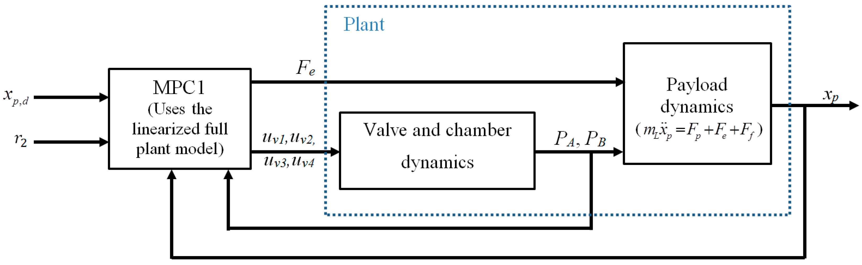
3.1. MPC1: Controller with Linearized Full Plant Model

Assuming that the full plant model of Section 2 and its parameters are known, an MPC law may be used for both position control and force allocation, outputting the electric force command and the inputs to the valves. The mass flow rates into the chambers are calculated using (6), which is a function of the upstream and downstream pressures. We term this approach MPC1. The controller structure is shown schematically in Figure 2.

The plant model must be linearized for use in the controller. The purpose of model linearization is to convert the nonlinear plant model into the linear discrete-time state space form of (10). The arguments k and k + 1 denote the kth and (k + 1)th samples.

$$\mathbf{x}(k+1)={\mathbf{A}}_{\mathbf{d}}\mathbf{x}(k)+{\mathbf{B}}_{\mathbf{d}}\mathbf{u}(k)+\mathbf{\upsilon }(k)$$

(10a)

$$\mathbf{y}(k)={\mathbf{C}}_{\mathbf{d}}\mathbf{x}(k)+{\mathbf{D}}_{\mathbf{d}}\mathbf{u}(k)$$

(10b)

To obtain the state space matrices (i.e., $A_{\mathbf{d}}, B_{\mathbf{d}}, {\mathbf{C}}_{\mathbf{d}},$ and ${\mathbf{D}}_{\mathbf{d}}$), Equations (1) and (4)–(6) are first used to derive the following vector equations:

$$\dot{\mathbf{x}}=f(\mathbf{x},\mathbf{u})$$

(11a)

$$\mathbf{y}=\mathbf{g}(\mathbf{x},\mathbf{u})$$

(11b)

Given (11), the continuous-time state space matrices can be calculated as shown in (12). The discrete-time matrices can be simply calculated by applying a discretization method to the matrices from (12). We used Euler’s method to obtain the matrices as shown in (13).

$${\mathbf{A}}_{\mathbf{c}}={\frac{\partial f}{\partial {\mathbf{x}}^T}|}_{op}$$

(12a)

$${\mathbf{B}}_{\mathbf{c}}={\frac{\partial f}{\partial {\mathbf{u}}^T}|}_{op}$$

(12b)

$${\mathbf{C}}_{\mathbf{c}}={\frac{\partial g}{\partial {\mathbf{x}}^T}|}_{op}$$

(12c)

$${\mathbf{D}}_{\mathbf{c}}={\frac{\partial g}{\partial {\mathbf{u}}^T}|}_{op}$$

(12d)

$${\mathbf{A}}_{\mathbf{d}}=I+T_s{\mathbf{A}}_{\mathbf{c}}$$

(13a)

$${\mathbf{B}}_{\mathbf{d}}=T_s{\mathbf{B}}_{\mathbf{c}}$$

(13b)

$${\mathbf{C}}_{\mathbf{d}}={\mathbf{C}}_{\mathbf{c}}$$

(13c)

$${\mathbf{D}}_{\mathbf{d}}={\mathbf{D}}_{\mathbf{c}}$$

(13d)

In (13a), $I$ is the identity matrix and $T_s$ is the controller sampling period. The full matrices are presented in Appendix A. The subscript “op” indicates linearization about an operating point. This is a point that includes states and inputs, as shown in (14).

$${\mathbf{x}}_{op}={\left[\begin{array}{cccc}{P}_A{}_{{}_{op}}& P_B{}_{{}_{op}}& x_p{}_{{}_{op}}& {\dot{x}}_{p_{op}}\end{array}\right]}^T$$

(14a)

$${\mathbf{u}}_{op}={\left[\begin{array}{cccc}{u}_{v{1}_{op}}& u_{v{2}_{op}}& u_{v{3}_{op}}& \begin{array}{cc}{u}_{v{4}_{op}}& F_{e_{op}}\end{array}\end{array}\right]}^T$$

(14b)

There are different options for selecting the operating point (14). One option is to use the current system states and input, i.e., $P_A{}_{{}_{op}}=P_A(k)$, $P_B{}_{{}_{op}}=P_B(k)$, $x_p{}_{{}_{op}}=x_p(k)$, ${\dot{x}}_{p_{op}}={\dot{x}}_p(k)$, $u_{v{i}_{op}}=u_{vi}(k-1)$, and $F_{e_{op}}=F_e(k-1)$. If this option is chosen, the operating point and the state space matrices need to be recalculated with every controller sampling period, passed to the MPC’s optimization solver, and then, kept constant within the prediction horizon. Note that the mass flow rate through each valve is modeled using distinct equations for the choked and unchoked modes (see (6)). Having four valves and each valve having two modes means there are 16 distinct versions of $f$ and $g$. With each iteration, the correct version of the functions must be chosen (depending on the valve modes) and used in (12) to update the state space matrices. This makes the resulting MPC too computationally complex to implement with common processors at the 10 ms or faster sampling period required for this application. To achieve a computationally feasible controller, we instead use a fixed operating point for the plant model linearization. This leads to only one version for each of the state space matrices (instead of the 16 versions with the dynamic operating point).

The following three assumptions are made to derive the linear model about a fixed operating point: (1) The states and inputs stay close enough to the operating point, (2) Valve spool time-constant (τ_v) is small enough compared to the controller sampling time that the spool’s dynamics can be neglected and z = u_v, and (3) Since the model is linearized about a constant operating point, the valve orifice area function in (7) may be replaced by a linear function of $A_v={\lambda }_{8}z+{\lambda }_9$ so that this single point will convey more information about the trend of the whole function. The state space state, input, and output vectors are shown below.

$$\mathbf{x}(k)={\left[\begin{array}{cccc}{P}_A(k)-P_A{}_{{}_{op}}& P_B(k)-P_B{}_{{}_{op}}& x_p(k)-x_p{}_{{}_{op}}& {\dot{x}}_p(k)-{\dot{x}}_{p_{op}}\end{array}\right]}^T$$

(15a)

$$\mathbf{u}(k)={\left[\begin{array}{cccc}{u}_{v1}(k)-u_{v{1}_{op}}& u_{v2}(k)-u_{v{2}_{op}}& u_{v3}(k)-u_{v{3}_{op}}& \begin{array}{cc}{u}_{v4}(k)-u_{v{4}_{op}}& F_e(k)\end{array}\end{array}-F_{e_{op}}\right]}^T$$

(15b)

$$\mathbf{y}(k)={\left[\begin{array}{cc}{x}_p(k)-x_p{}_{{}_{op}}& \frac{(P_A(k)-P_A{}_{{}_{op}})+(P_B(k)-P_B{}_{{}_{op}})}{2}\end{array}\right]}^T$$

(15c)

From (3), it can be seen that the cylinder can have infinite combinations of chamber pressures that produce the same pneumatic force. The strategy behind defining the second output is to limit the pressure choices by keeping the average of chambers pressures near $P_{mid}=\left(P_s+P_{atm}\right)/2$, which means requiring the second output to track a constant reference of $r_2=P_{mid}-\left(P_A{}_{{}_{op}}+P_B{}_{{}_{op}}\right)/2$. In this paper, the operating point elements have been picked as ${\mathbf{u}}_{op}=0$, $x_p{}_{{}_{op}}=0$, and ${\dot{x}}_{p_{op}}=0$. The operating points for chamber pressures have been chosen such that they satisfy $(P_A{}_{{}_{op}}-P_{atm})A_A-(P_B{}_{{}_{op}}-P_{atm})A_B=0$ and $\left(P_A{}_{{}_{op}}+P_B{}_{{}_{op}}\right)/2=P_{mid}$. Therefore, the pressure operating points are:

$$P_A{}_{{}_{op}}=\frac{2P_{mid}+\left(\frac{A_A}{A_B}-1\right)P_{atm}}{\frac{A_A}{A_B}+1}$$

(16a)

$$P_B{}_{{}_{op}}=\frac{2P_{mid}+\left(\frac{A_B}{A_A}-1\right)P_{atm}}{\frac{A_B}{A_A}+1}$$

(16b)

The MPC1 law uses (10) to predict the future states. It solves the optimization problem (17) every sampling instant with a prediction horizon of N_p points, by using a time-efficient convex optimization algorithm. In (17), k is the current sample number, $r={\left[\begin{array}{cc}{x}_{p,d}& r_2\end{array}\right]}^T$ is the vector of the two reference inputs, and Q, R₁, and R₂ are positive-definite gain matrices.

$$\begin{array}{ll}\begin{array}{c}minimize\\ \mathbf{u}\end{array}& {\displaystyle \sum _{i=1}^{N_p}({(\mathbf{y}(k+i)-\mathbf{r}(k+i))}^T\mathbf{Q}(\mathbf{y}(k+i)-\mathbf{r}(k+i))\dots }\\ & \hspace{1em}+{(\mathbf{u}(k+i))}^T{\mathbf{R}}_1\mathbf{u}(k+i)+{(\mathbf{u}(k+i)-\mathbf{u}(k+i-1))}^T{\mathbf{R}}_2(\mathit{u}(k+i)-\mathbf{u}(k+i-1))\\ subject to& \\ & \mathbf{x}(k+j+1)=A_{d}x(k+j)+B_{d}u(k+j)+T_{s}f({\mathbf{x}}_{op},{\mathbf{u}}_{op})\hspace{1em},j=0,\dots ,N_p-1\\ & y(k+j)=C_{d}x(k+j)+D_{d}u(k+j)\hspace{1em},j=1,\dots ,N_p\\ & u_{\min }\le u(k+j)\le u_{\max }\hspace{1em},j=1,\dots ,N_p\\ & x_{\min }\le \mathit{x}(k+j)\le x_{\max }\hspace{1em},j=1,\dots ,N_p\end{array}$$

(17)

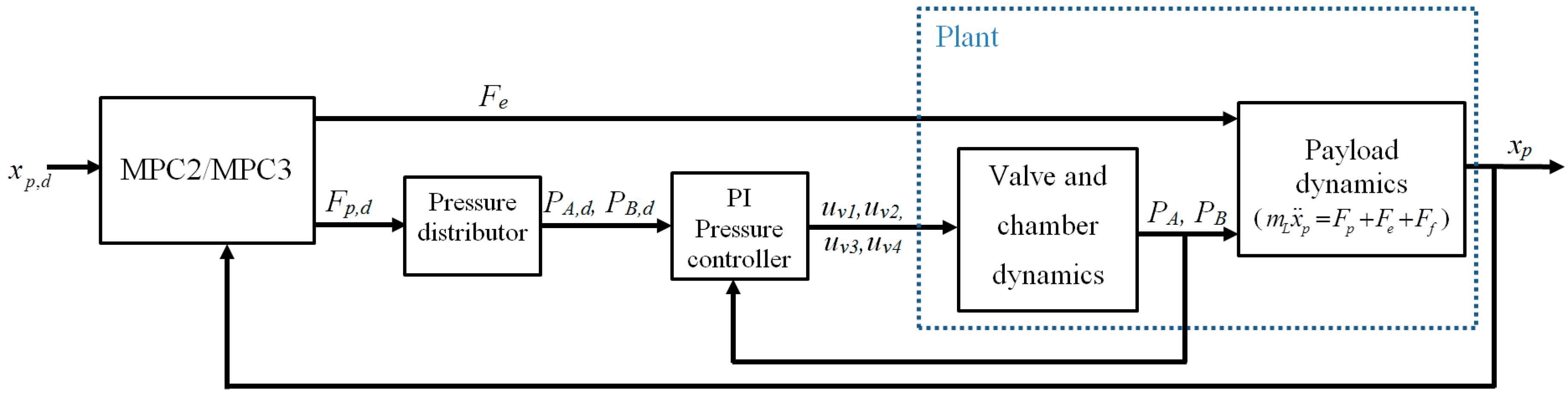
3.2. MPC2: Simplified Two-Loop Controller

The MPC1 approach must solve an optimization problem every sampling period, which is computationally expensive since it includes models of both the payload dynamics and pneumatic dynamics. As a faster alternative, with our second approach, termed MPC2, the MPC law neglects the dynamics of the pneumatic subsystem. In other words, the MPC2 law assumes the actual pneumatic force equals its desired value, i.e., $F_p=F_{p,d}$. This design requires a two-loop controller structure as the MPC2 block is responsible for controlling the position subsystem solely. An inner-loop pressure controller handles the pneumatic subsystem and defines the command signals for each valve. The schematic of this control system structure is illustrated in Figure 3.

MPC2 uses (1) to derive linear state space model as in (11) with the following states, inputs, and output. The corresponding state space model matrices are presented in Appendix A.

$$x(k)={\left[\begin{array}{cc}{x}_{p(k)}& {\stackrel{·}{x}}_{p(k)}\end{array}\right]}^T$$

(18a)

$$u(k)={\left[\begin{array}{cc}{F}_{p,d(k)}& F_{e(k)}\end{array}\right]}^T$$

(18b)

$$y(k)=x_p{}_{(k)}$$

(18c)

The optimization problem declaration is almost the same as MPC1, with the only difference being adding one more constraint (shown in (19)) to limit the changes in u(k) between two consecutive samples. This change is necessary as MPC2 ignores the inner dynamics of the pressure subsystems and its limitations.

$$\Delta u_{\min }\le u(k+j)-u(k+j-1)\le \Delta u_{\max }\hspace{1em},j=1,\dots ,N_p$$

(19)

Before feeding $F_{p,d}$ from the outer-loop position controller to the inner-loop pressure controller, the pressure distributor should define the desired chamber pressures. This is done by satisfying the two conditions $(P_{A,d}(k)-P_{atm})A_A-(P_{B,d}(k)-P_{atm})A_B=F_{p,d}(k)$ and $\left(P_{A,d}(k)+P_{B,d}(k)\right)/2=P_{mid}$. The solution to these conditions is shown in (20).

$$P_{A,d(k)}=\frac{2P_{mid}+\left(\frac{A_A}{A_B}-1\right)P_{atm}+\frac{F_{p,d(k)}}{A_B}}{\frac{A_A}{A_B}+1}$$

(20a)

$$P_{B,d(k)}=\frac{2P_{mid}+\left(\frac{A_B}{A_A}-1\right)P_{atm}-\frac{F_{p,d(k)}}{A_A}}{\frac{A_B}{A_A}+1}$$

(20b)

A conventional PI controller, with a bounded trapezoidal integral term, is used to control chamber pressures as shown in (21). Here, $\mathsf{\Gamma }$ denotes the integral bound.

$$u_j(k)=K_{p,p}\left(P_{j,d}(k)-P_j(k)\right)+\min \left(\mathsf{\Gamma },\max \left({\phi }_j(k),-\mathsf{\Gamma }\right)\right)\hspace{1em}, j\in \left\{A,B\right\}$$

(21)

where ${\phi }_j(k)=K_{I,p}\frac{T_s}{2}{\displaystyle \sum _{\eta =2}^k\left(P_{j,d}(\eta )-P_j(\eta )+P_{j,d}(\eta -1)-P_j(\eta -1)\right)}$.

The pressure controller in (21) returns a value for $u_j$ that needs to be normalized and distributed between the charging and discharging valves. To do so, the distributor function, $\mathsf{\Omega }$, is used as follows.

$$\left[u_{v1}(k),u_{v2}(k)\right]=\mathsf{\Omega }\left(u_A(k)\right)$$

(22a)

$$\left[u_{v3}(k),u_{v4}(k)\right]=\mathsf{\Omega }\left(u_B(k)\right)$$

(22b)

where $\mathsf{\Omega }\left(\epsilon \right)=\{\begin{array}{ll}\left[\min (\epsilon ,1),0\right]& \epsilon \ge 0\\ \left[0,\min (-\epsilon ,1)\right]& \epsilon <0\end{array}$.

3.3. MPC3: Modified Two-Loop Controller

MPC1 and MPC2 are two extremes in terms of dynamic models for the pneumatic subsystem. MPC1 uses a linearized model of the pneumatic dynamics, whereas MPC2 neglects these dynamics. The MPC law proposed in this section, termed MPC3, is a compromise between these two extremes that is intended to balance the trade-off between performance and controller computation time. The controller structure of Figure 3 with the independent pressure controller is adopted, but the MPC position controller is expanded to include a simplified model of the pneumatic dynamics.

To obtain the simplified model for predicting the pneumatic force, $F_p$, we assume that the proportional term in (21) is dominant and that the derivative of each cylinder chamber pressure is approximately proportional to its associated valve command signal, i.e.,

$${\dot{P}}_A\cong \mathsf{\Psi }{u}_A\cong \mathsf{\Psi }{K}_{p,p}\left(P_{A,d}-P_A\right)$$

(23a)

$${\dot{P}}_B\cong \mathsf{\Psi }{u}_B\cong \mathsf{\Psi }{K}_{p,p}\left(P_{B,d}-P_B\right)$$

(23b)

Substituting (23) into (3) then gives the following simplified dynamic model for the pneumatic force:

$${\dot{F}}_p=\kappa (F_{p,d}-F_p)$$

(24)

Finally, the discretized form of (24) is added to the state space model of MPC2 to produce the state space model used by MPC3. Its state vector is defined by (25). Its input vector and output are defined by (18a) and (18b), respectively. The corresponding state space model matrices are presented in Appendix A.

$$x(k)={\left[\begin{array}{ccc}{x}_p{}_{(k)}& {\dot{x}}_{p(k)}& F_{p(k)}\end{array}\right]}^T$$

(25)

3.4. Linear Two-Loop Controller

As a comparison benchmark, a conventional linear position controller was also designed and simulated. The controller structure is the same as that of Figure 3, except the MPC2 block is replaced with a linear position controller. This controller structure is similar to the two-loop structure used in [3]. Two independent controllers are used with the pneumatic and the electric actuators, with the former using feedforward + PD controller and the latter using a PD controller. Since the electric actuator has a faster response but significantly lower force capacity, the feedforward terms that compensate for the modeled inertial and friction forces are fed to the pneumatic actuator controller, while the electric actuator’s force capacity is saved for reducing the residual error. The equations for these controllers are shown in (26) and (27).

$$F_{p,d}(k)=m_L{\ddot{x}}_{p,d}(k)+{\widehat{C}}_v{\dot{x}}_p(k)+K_{P,c}\left(x_{p,d}(k)-x_p(k)\right)+K_{D,c}\left({\dot{x}}_{p,d}(k)-{\dot{x}}_p(k)\right)$$

(26)

$$F_e(k)=K_{P,m}\left(x_{p,d}(k)-x_p(k)\right)+K_{D,m}\left({\dot{x}}_{p,d}(k)-{\dot{x}}_p(k)\right)$$

(27)

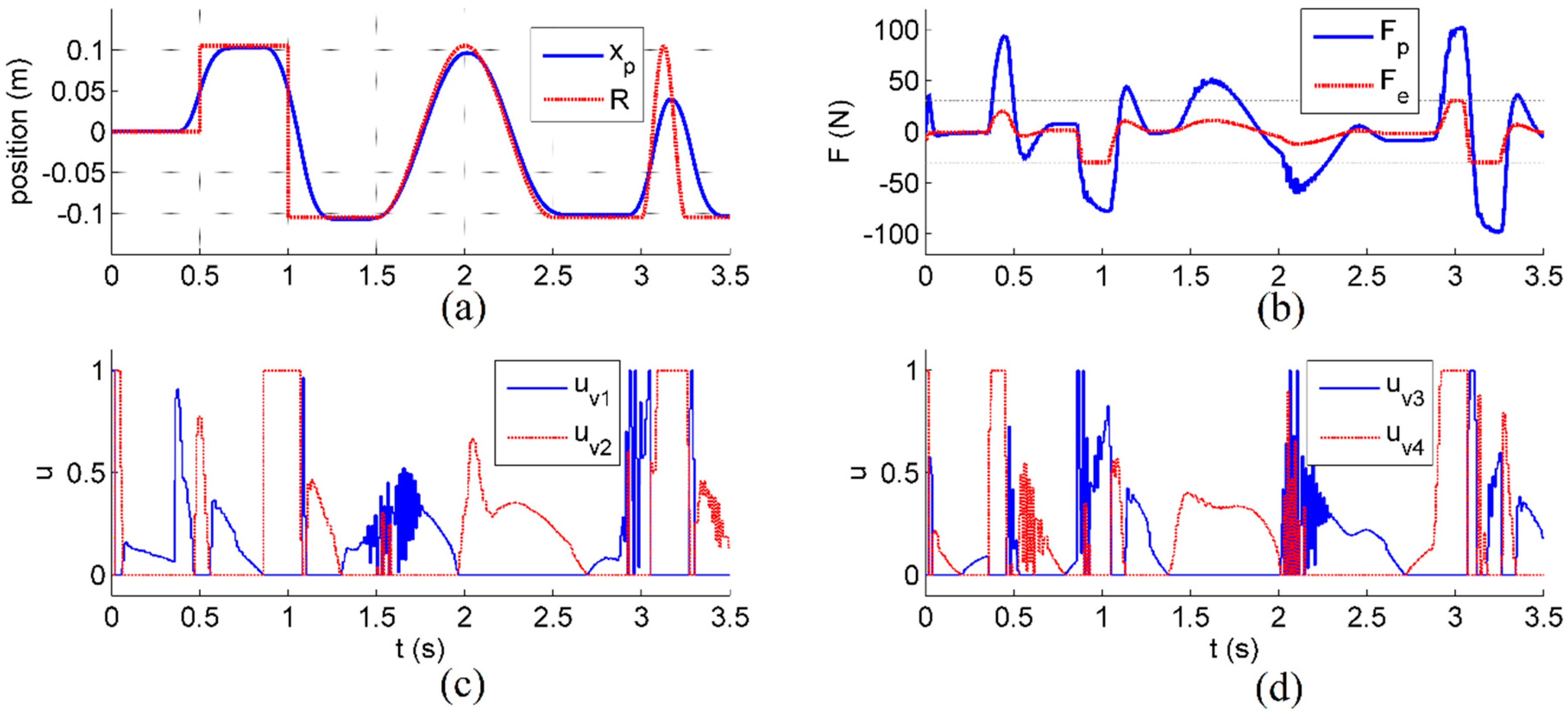
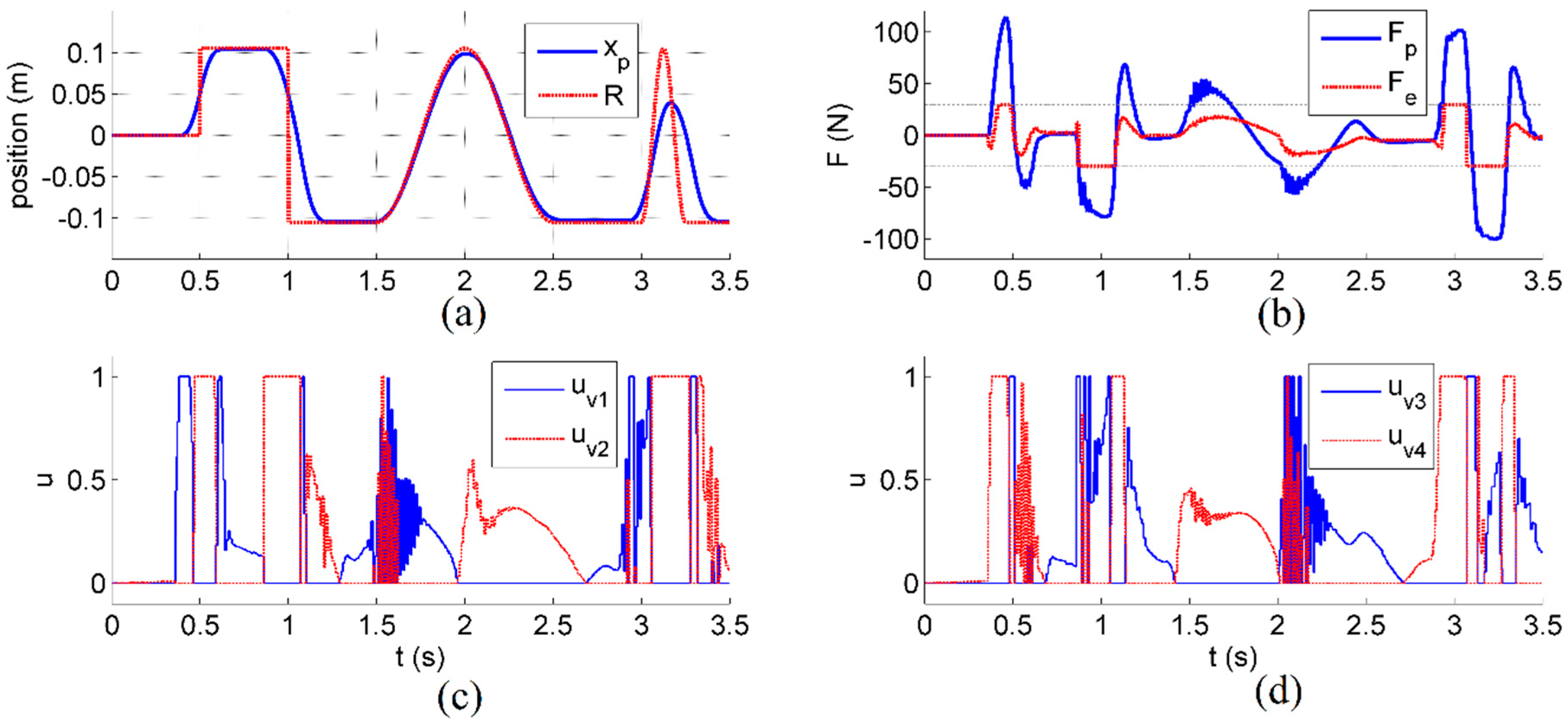
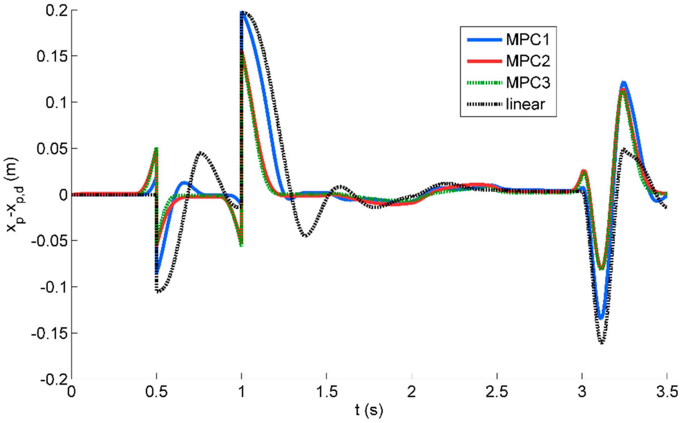
4. Results and Discussion

The four controllers were simulated using MATLAB m code and Yalmip [16] running on a Windows 10 PC with an Intel Core i5 processor. To challenge the tracking and force allocation performance, a relatively large payload mass of $m_L=$10 kg was used. The pneumatic actuator parameters for an SMC CM2XB25-300 air cylinder [19] and an Enfield LS-V05s pneumatic valve [20] were employed. The simulated linear motor is an Aerotech BLMC-92. To prevent motor overheating, the electric actuator’s force has been limited to 30 N, which is lower than the 44.5 N continuous force rating of this Aerotech motor. All controller parameters were manually tuned with the goal of minimizing the root-mean-square error (RMSE). This tuning employed a coarse search followed by a fine search to reduce the possibility of stopping at a local minima.

Table 1. Plant and controller parameters.

Parameter	Value	Parameter	Value
$A_A$	4.909 × 10−4 m2	$\mathbf{Q}$ (MPC3)	106
$A_B$	4.123 × 10−4 m2	$R$	287 J/kg·K
$C_1$	0.040418	${\mathbf{R}}_1$ (MPC1)	diag([1, 1, 1, 1, 10−3])
$C_2$	0.156174	${\mathbf{R}}_1$ (MPC2)	diag([0.1, 0.5])
$C_f$	0.5393	${\mathbf{R}}_1$ (MPC3)	diag([0.1, 0.5])
$C_v$	44.4 N·s/m	${\mathbf{R}}_2$ (MPC1)	0
$F_{kf}$	13 N	${\mathbf{R}}_2$ (MPC2)	diag([0.1, 0])
$F_{sf}$	18 N	${\mathbf{R}}_2$ (MPC3)	diag([0.1, 0])
$K$	1.4	$T$	293 K
$K_{P,c}$	2000 N/m	Numerical integration timestep	0.0005 s
$K_{D,c}$	30 N·s/m	$\Delta u_{\min }$ (MPC2)	[−30, −60]T
$K_{P,m}$	500 N/m	$\Delta u_{\max }$ (MPC2)	[30, 60]T
$K_{D,m}$	50 N·s/m	$\mathsf{\Gamma }$	5000 Pa·s
$K_{p,p}$	5 × 10−5 Pa−1	$\kappa$	70
$K_{I,p}$	5 × 10−4 Pa−1s−1	${\lambda }_1$	0.585
$L_S$	0.3 m	${\lambda }_2$	−7.51
$L_{DV}$	0.03 m	${\lambda }_3$	38.1
$m_L$	10 kg	${\lambda }_4$	−46.9
$N_P$	15	${\lambda }_5$	18.2
$P_{atm}$	101,000 Pa	${\lambda }_6$	−21.3
$P_{cr}$	0.528	${\lambda }_7$	3.42
$P_s$	404000 Pa	${\lambda }_8$	5 × 10−5
$\mathbf{Q}$ (MPC1)	diag([104, 10−3])	${\lambda }_9$	0
$\mathbf{Q}$ (MPC2)	106	${\tau }_v$	0.0015 s

lists the parameters used.

To keep the models within the MPC-based controllers in linear time-invariant form, the static and kinetic friction components are treated as unmodeled disturbances. Only the viscous friction is incorporated in the MPC models, for which a 20% uncertainty is included in the friction coefficient ${\widehat{C}}_v$ (i.e., ${\widehat{C}}_v=0.8C_v$). Figure 4, Figure 5, Figure 6 and Figure 7 show the results from each controller. They follow a reference trajectory made up of step inputs, a 1 Hz sine wave, then a faster 4 Hz sine wave. This trajectory was chosen to be challenging and led to multiple saturations of the valve commands and electric actuator force (at 1 and 30 N, respectively), as shown in Figure 4, Figure 5, Figure 6 and Figure 7. For easier comparison, the tracking errors are plotted on the same axes in Figure 8.

From Figure 4, Figure 5, Figure 6, Figure 7 and Figure 8, it can be seen that the linear controller has a longer settling time, bigger overshoot, and larger error peaks when subjected to the faster trajectories, such as 4 Hz. However, all MPC-based controllers undergo chattering in the actuator force at some points, while the linear controller produces the smoothest input force and valve commands, which may lead to longer valve and actuator lives in practice. Between the MPC-based controllers, MPC3 produced the most accurate position tracking. A quantitative comparison is presented in

Table 2. Numerical comparison of the controller results.

Parameter	Value
	MPC1	MPC2	MPC3	Linear
Sampling period (Ts)	10 ms	10 ms	10 ms	1 ms
Position tracking RMSE	44.7 mm	29.9 mm	23.9 mm	53.0 mm
Mean Absolute Fp	29.73 N	28.11 N	28.81 N	33.58 N
Mean Absolute Fe	11.74 N	7.78 N	11.12 N	12.24 N
Average calculation time per sample	4.5 ms	3.9 ms	4.3 ms	0.003 ms
Maximum calculation time per sample	8.5 ms	6.4 ms	7.2 ms	0.02 ms

. Although the linear controller has the lowest accuracy of the three, it has a much faster calculation time. MPC1 requires the highest calculation time which is undesirable for real-time operation. MPC3 yields the best tracking performance with RMSE reduction of 46%, 20%, and 55% compared to MPC1, MPC2, and the linear controller, respectively. MPC3 also reduced the mean absolute electric actuator force by 9%, and the mean absolute pneumatic actuator force by 14% relative to the benchmark linear controller. These force reductions have the benefits of reducing the energy consumption and operating cost.

5. Conclusions

In this paper, three novel control algorithms for the position control of an HPEA-driven system are investigated. The first (MPC1) uses MPC with a linearized full plant model. The second (MPC2) uses an outer-loop MPC with an inner-loop PI pressure controller with a simplified linear model. The third (MPC3) uses the same structure as MPC2 with a modified model to find a balance in the trade-off between the position controller performance and computation time. A fourth controller, employed as a benchmark, uses an outer-loop PD plus feedforward controller with an inner-loop PI pressure controller. MPC2 showed the best performance in reducing the input forces (and thus, the energy consumption and operating cost). However, modifying the model in MPC3 leads to the best position tracking performance. Although MPC2 and MPC3 are computationally intensive, they can still be run in real-time using commonly available off-the-shelf hardware.

This research will be continued by investigating the extension of the MPC-based position control and task allocation approaches to rotary HPEA actuators with nonlinear payload dynamics. To avoid the subjectivity of the manual tuning approach, we will also be investigating the application of global optimization strategies (such as particle swarm optimization) to obtain the controller parameters.

References

1. ISO/TS 15066:2016. Robots and Robotic Devices-Collaborative Robots; International Organization for Standardization: Geneva, Switzerland, 2016. [Google Scholar]
2. Shin, D.; Sardellitti, I.; Khatib, O. A hybrid actuation approach for human-friendly robot design. In Proceedings of the 2008 IEEE International Conference on Robotics and Automation, Pasadena, CA, USA, 19–23 May 2008; pp. 1747–1752. [Google Scholar]
3. Rouzbeh, B.; Bone, G.; Ashby, G.; Li, E. Design, Implementation and Control of an Improved Hybrid Pneumatic-Electric Actuator for Robot Arms. IEEE Access 2019, 7, 14699–14713. [Google Scholar] [CrossRef]
4. Petrosky, L.J. Hybrid Electro-Pneumatic Robot Joint Actuator. U.S. Patent 478 225 828, 1 November 1988. [Google Scholar]
5. Takemura, F.; Pandian, S.R.; Nagase, Y.; Mizutani, H.; Hayakawa, Y.; Kawamura, S. Control of a hybrid pneumatic/electric motor. In Proceedings of the 2000 IEEE/RSJ International Conference on Intelligent Robots and Systems (IROS 2000) (Cat No 00CH37113) IROS-00, Takamatsu, Japan, 31 October–5 November 2002; Volume 1, pp. 209–214. [Google Scholar]
6. Teramae, T.; Noda, T.; Hyon, S.-H.; Morimoto, J.; Noda, T. Modeling and control of a Pneumatic-Electric hybrid system. In Proceedings of the 2013 IEEE/RSJ International Conference on Intelligent Robots and Systems, Tokyo, Japan, 3–7 November 2013; Volume 4, pp. 4887–4892. [Google Scholar]
7. Ishihara, K.; Morimoto, J. An optimal control strategy for hybrid actuator systems: Application to an artificial muscle with electric motor assist. Neural Netw. 2018, 99, 92–100. [Google Scholar] [CrossRef] [PubMed]
8. Sharbafi, M.A.; Shin, H.; Zhao, G.; Hosoda, K.; Seyfarth, A. Electric-Pneumatic Actuator: A New Muscle for Locomotion. Actuators 2017, 6, 30. [Google Scholar] [CrossRef] [Green Version]
9. Bone, G.; Chen, X. Position control of hybrid pneumatic-electric actuators. In Proceedings of the 2012 American Control Conference (ACC), Montreal, QC, Canada, 27–29 June 2012; pp. 1793–1799. [Google Scholar]
10. Bone, G.; Xue, M.; Flett, J. Position control of hybrid pneumatic–electric actuators using discrete-valued model-predictive control. Mechatronics 2015, 25, 1–10. [Google Scholar] [CrossRef]
11. Nakata, Y.; Noda, T.; Morimoto, J.; Ishiguro, H. Development of a pneumatic-electromagnetic hybrid linear actuator with an integrated structure. In Proceedings of the 2015 IEEE/RSJ International Conference on Intelligent Robots and Systems (IROS), Hamburg, Germany, 28 September–2 October 2015; pp. 6238–6243. [Google Scholar]
12. Mori, S.; Tanaka, K.; Nishikawa, S.; Niiyama, R.; Kuniyoshi, Y. High-Speed Humanoid Robot Arm for Badminton Using Pneumatic-Electric Hybrid Actuators. IEEE Robot. Autom. Lett. 2019, 4, 3601–3608. [Google Scholar] [CrossRef]
13. Johansen, T.A.; Fossen, T.I. Control allocation-A survey. Automatica 2013, 49, 1087–1103. [Google Scholar] [CrossRef] [Green Version]
14. Härkegård, O. Dynamic Control Allocation Using Constrained Quadratic Programming. J. Guid. Control. Dyn. 2004, 27, 1028–1034. [Google Scholar] [CrossRef] [Green Version]
15. Galeani, S.; Pettinari, S. On dynamic input allocation for fat plants subject to multi-sinusoidal exogenous inputs. In Proceedings of the 53rd IEEE Conference on Decision and Control, Los Angeles, CA, USA, 15–17 December 2014; pp. 2396–2403. [Google Scholar]
16. Lofberg, J. YALMIP: A toolbox for modeling and optimization in MATLAB. In Proceedings of the 2004 IEEE International Conference on Robotics and Automation (IEEE Cat No 04CH37508) CACSD-04, New Orleans, LA, USA, 2–4 September 2005; pp. 284–289. [Google Scholar]
17. Mattingley, J.; Boyd, S. CVXGEN: A code generator for embedded convex optimization. Optim. Eng. 2011, 13, 1–27. [Google Scholar] [CrossRef]
18. Hanger, M.; Johansen, T.A.; Mykland, G.K.; Skullestad, A. Dynamic model predictive control allocation using CVXGEN. In Proceedings of the 2011 9th IEEE International Conference on Control and Automation (ICCA), Santiago, Chile, 19–21 December 2011; pp. 417–422. [Google Scholar]
19. Ning, S.; Bone, G. Development of a nonlinear dynamic model for a servo pneumatic positioning system. In Proceedings of the IEEE International Conference Mechatronics and Automation, Niagara Falls, ON, Canada, 29 July–1 August 2005; pp. 43–48. [Google Scholar]
20. Taheri, B.; Case, D.; Richer, E. Force and Stiffness Backstepping-Sliding Mode Controller for Pneumatic Cylinders. IEEE/ASME Trans. Mechatronics 2014, 19, 1799–1809. [Google Scholar] [CrossRef]
21. Richer, E.; Hurmuzlu, Y. A High Performance Pneumatic Force Actuator System: Part I—Nonlinear Mathematical Model. J. Dyn. Syst. Meas. Control. 1999, 122, 416–425. [Google Scholar] [CrossRef]
Figure 1. Schematic illustration of the HPEA-driven system.
Actuators 09 00086 g001
Figure 2. Controller structure used with MPC1.
Actuators 09 00086 g002
Figure 3. Controller structure used with MPC2 and MPC3.
Actuators 09 00086 g003
Figure 4. Position tracking and force allocation performance using MPC1: (a) position tracking, (b) actuator forces, (c) command to the valves controlling chamber A, and (d) command to the valves controlling chamber B.
Actuators 09 00086 g004
Figure 5. Position tracking and force allocation performance using MPC2: (a) position tracking, (b) actuator forces, (c) command to the valves controlling chamber A, and (d) command to the valves controlling chamber B.
Actuators 09 00086 g005
Figure 6. Position tracking and force allocation performance using MPC3: (a) position tracking, (b) actuator forces, (c) command to the valves controlling chamber A, and (d) command to the valves controlling chamber B.
Actuators 09 00086 g006
Figure 7. Position tracking and force allocation performance using the linear controller: (a) position tracking, (b) actuator forces, (c) command to the valves controlling chamber A, and (d) command to the valves controlling chamber B.
Actuators 09 00086 g007
Figure 8. Comparison of the position tracking errors with the four control laws.
Actuators 09 00086 g008