Run-Disjoint Few-Shot XGBoost Framework for Compound Fault Diagnosis of Induction Motors

Abstract

Few-shot compound fault diagnosis of induction motors can be overestimated when correlated windows from the same continuous run are split across support and query sets. This study develops a run-disjoint few-shot framework in which each complete experimental run is treated as one shot and support and query sets are separated by run ID. Forty-eight multidomain features are extracted from synchronized triaxial vibration windows, classified using task-specific XGBoost, and aggregated to obtain run-level predictions; TreeSHAP provides post hoc feature attribution. In a matched comparison with identical query runs and windows, window-mixed partitioning increased the task-level mean run-level Macro-F1 from 0.9212 to 0.9934. After repeated predictions were aggregated over 108 unique query runs, the corresponding difference was 0.0093 with a 95% paired-bootstrap confidence interval of [0.0000, 0.0282], showing that the estimated magnitude depends on the statistical unit. Under the predefined strict 3-shot protocol, XGBoost achieved a Macro-F1 of 0.9263 and run-level accuracy of 0.9292. Additional sensitivity and controlled comparisons showed that performance depends on within-run sampling, representation, and classifier design, while strict cross-speed tests revealed the limitation of fixed-frequency features under rotational-speed shifts. The framework provides a leakage-aware evaluation procedure for few-shot compound-fault diagnosis using independently labeled runs.

1. Introduction

Induction motors are key power components in industrial drive systems and serve as electromechanical actuators in pumps, fans, compressors, conveying mechanisms, and automated equipment. Faults involving bearings, rotors, stator windings, and eccentricity can directly affect the output stability, tracking performance, and operational reliability of actuator systems. Therefore, compound fault diagnosis of induction motors under variable-speed and variable-load conditions is an important basis for condition monitoring and predictive maintenance in electric-drive actuator systems.

Previous studies have systematically reviewed the mechanisms, observable signals, and diagnostic methods associated with typical induction motor faults, including bearing damage, broken rotor bars, stator winding abnormalities, and eccentricity [1,2]. Localized rolling-element bearing defects generally produce periodic impacts and modulation components in vibration signals, for which vibration analysis and envelope demodulation are commonly used as condition-monitoring techniques [3]. With the development of artificial intelligence and machine learning, data-driven methods have been widely applied to fault diagnosis of motors and rotating machinery and have gradually progressed toward actuator-system integration, adaptation to variable operating conditions, and interpretable analysis [4,5]. Recent surveys have further summarized conventional machine learning methods and emerging deep learning architectures for rotating-machinery fault diagnosis, highlighting the increasing role of data-driven models in automated condition monitoring and intelligent maintenance [6]. During long-term operation, bearing damage, broken rotor bars, eccentricity, and winding abnormalities may occur either individually or simultaneously because of mechanical, electromagnetic, and load coupling. Compared with single faults, compound faults generally involve the superposition, modulation, or mutual masking of multiple fault signatures. Consequently, the distinctions among different fault combinations become less clear, increasing the difficulty of actuator-system condition monitoring and maintenance decision-making.

Deep learning can directly learn hierarchical fault representations from raw vibration signals, spectra, or time–frequency representations, thereby reducing its dependence on manually designed features. However, stable performance usually relies on sufficiently large labeled datasets and relatively consistent training and test distributions [7]. Compound fault experiments require the artificial configuration of different faulty components and severity levels, resulting in high data acquisition costs. For some newly encountered fault combinations, only a few complete experimental runs may be available. In addition, differences in speed or load may exist between labeled support runs and the runs to be diagnosed, violating the identically distributed assumption commonly adopted by supervised models. When only a few independently labeled runs are available for a target compound fault, it becomes particularly difficult to establish class boundaries that are robust to operating-condition variations.

Recent studies have also explored more sophisticated multisensor representation-learning and feature-fusion strategies for rotating-machinery diagnosis. For example, Li et al. developed a multi-branch parallel perception and feature-fusion framework to exploit complementary information from multiple bearing-monitoring sensors [8]. Such advances improve the quality of diagnostic representations, but representation learning or sensor fusion alone does not resolve the evaluation dependence that arises when multiple correlated windows from one physical acquisition are treated as independent few-shot observations.

Few-shot learning provides a potential solution when only a small number of labeled fault observations are available. However, in rotating-machinery diagnosis, the validity of few-shot evaluation depends not only on the learning algorithm but also on how a “shot” is physically defined. A continuous acquisition run is commonly segmented into multiple local windows, which share the same fault configuration, operating condition, sensor installation, and acquisition background. Consequently, these windows should not be interpreted as mutually independent fault observations.

Data leakage caused by correlated samples and the need for group-wise validation have been recognized in previous studies. The specific gap addressed here is therefore not the general concept of grouped data partitioning itself. Rather, it concerns its implementation in few-shot fault diagnosis, where local windows from one physical acquisition may be counted as multiple shots or distributed across support and query sets. Under such a protocol, the nominal number of shots does not correspond to the number of independently labeled fault experiments, and the resulting few-shot performance may not represent generalization to unseen acquisition runs.

To address this specific evaluation issue, this study defines one independently acquired experimental run as one shot and separates the support and query sets at the run-ID level. In addition, a matched-query experiment is constructed in which the query runs, query windows, and support-window budget are held fixed, allowing the performance inflation caused specifically by window-level mixing to be quantified.

Based on the above literature, three specific gaps motivate the present study. First, the physical acquisition unit represented by a “shot” is not always explicitly distinguished from the local signal windows extracted from that acquisition. Second, the performance inflation caused by violating run-level support–query independence has rarely been quantified under strictly matched query conditions using the unique physical run as the statistical unit. Third, comparisons among few-shot diagnostic methods may simultaneously change the input representation, classifier design, and amount of prior source training, making their individual effects difficult to distinguish.

To address these gaps, the main contributions of this study are summarized as follows:

(1) A run-disjoint few-shot evaluation protocol is established by defining one independently acquired experimental run as one shot. A matched-query comparison is further designed to quantify leakage-induced performance inflation while keeping the query runs, query windows, and support-window budget unchanged.

(2) A common-query evaluation procedure is implemented using compound-fault class rotation, repeated support episodes, unique-run-level statistical inference, and controlled cross-speed and cross-load separation. This design evaluates few-shot generalization without treating correlated windows as independent physical observations.

(3) The proposed protocol is instantiated using a lightweight diagnostic workflow consisting of synchronized triaxial multidomain features, task-specific XGBoost classification, within-run aggregation, and TreeSHAP-based post hoc feature attribution.

2. Related Work

2.1. Compound Fault Diagnosis of Induction Motors

Existing methods for induction motor fault diagnosis mainly include conventional approaches based on manually engineered features and data-driven approaches based on deep representations. Conventional methods generally extract time-domain, frequency-domain, and time–frequency indicators from vibration, current, torque, or magnetic-flux signals and then identify equipment states using statistical analysis or shallow classifiers. Indicators such as root mean square, peak-to-peak value, crest factor, skewness, kurtosis, envelope spectrum, band energy, and fault characteristic frequencies can characterize vibration amplitude, impact behavior, and changes in spectral structure. These methods offer advantages such as physically interpretable features, low computational cost, and ease of engineering deployment. Nevertheless, their performance generally depends on manual feature selection, signal-preprocessing strategies, and empirical knowledge associated with specific operating conditions.

With the development of deep learning, convolutional neural networks, deep belief networks, Transformers, and graph neural networks have increasingly been used to automatically learn fault representations from raw vibration sequences, spectra, or time–frequency representations. Ince et al. directly applied a one-dimensional convolutional neural network to real-time motor fault identification, demonstrating the feasibility of end-to-end temporal modeling for online motor monitoring [9]. To address limited labeled data and load variations, Chang et al. developed a residual VGG-based Siamese network that improved cross-load induction motor diagnosis through few-shot similarity learning [10]. Shao et al. used a deep belief network to learn the frequency-distribution characteristics of induction motor vibration signals [11], whereas Lee et al. demonstrated the effectiveness of convolutional neural networks for classifying rotor and bearing faults in induction motors [12].

With advances in sequence modeling and multisensor relational learning, Jin et al. proposed a time-series Transformer method for rotating-machinery fault diagnosis to capture long-range dependencies in vibration sequences [13]. Li et al. subsequently employed a multiview graph neural network to fuse information from different sensors and feature views, thereby improving diagnostic robustness in noisy environments [14]. These studies demonstrate that deep models can learn complex patterns involving local impacts, frequency modulation, and cross-temporal-scale dependencies and can achieve high diagnostic performance when sufficient training samples are available and the training and test distributions are similar. However, high-capacity deep models generally require substantial labeled data, and their performance may still deteriorate considerably when the target equipment, sensor configuration, or operating conditions change.

To address the superposition, coupling, and mutual masking of multiple fault signatures in compound fault conditions, previous studies have investigated multisource information fusion, multilabel classification, tree-ensemble learning, and cross-domain representation learning. Gong et al. fused multisource current and vibration signals and employed a multichannel deep convolutional network to identify motor compound faults [15]. Their subsequent study combined inverse graph Fourier transforms, a multihead convolutional neural network, and a multilabel decoupling classifier to improve the identification of strongly coupled motor compound faults [16]. In addition to deep models, Alhams et al. compared Decision Tree, Random Forest, and XGBoost for vibration-based fault diagnosis and used feature-importance analysis to interpret the discriminative basis of the tree-ensemble models [17]. Shen et al. developed a deep multilabel learning framework to jointly represent multiple fault components that may coexist in a sample [18]. More recently, Pu et al. investigated joint-distribution alignment for compound fault diagnosis under unseen operating conditions from a domain-generalization perspective, reducing the effect of operating-condition changes on the boundaries between compound fault classes [19].

These studies demonstrate the effectiveness of multisource fusion, deep feature learning, and multilabel modeling for compound fault recognition. Nevertheless, most existing methods assume that sufficiently large amounts of target compound fault data are available during training or that the training and test data are collected under the same or similar operating conditions. Scenarios in which only a few independently labeled runs are available for each new compound fault remain insufficiently investigated.

2.2. Motor Fault Diagnosis Under Variable Operating Conditions

Practical electromechanical actuator systems commonly operate under varying speeds and loads. Speed variations shift rotational and fault-related frequencies, whereas load variations affect vibration amplitudes, impact intensities, and fault-signature observability. These changes can produce substantial distribution shifts even under the same fault state and have motivated extensive research on transfer learning, domain adaptation, adversarial learning, and distribution alignment [20,21,22,23,24,25,26,27]. Recent studies have further investigated motor fault diagnosis across variable loads, rotational speeds, and torque conditions using subdomain adaptation, variable-condition generalization, and self-supervised feature learning [28,29,30]. These studies further demonstrate that motor fault diagnosis under changing operating conditions is an established research topic. However, most existing methods rely on abundant labeled source data, target-domain adaptation, domain-generalization training, or condition-invariant representation learning.

In contrast, this study focuses on task-specific diagnosis using only a few run-ID-disjoint support runs. The main tasks include multiple speeds and loads without requiring complete operating-condition separation, while additional controlled experiments impose strictly nonoverlapping support and query speeds or loads to evaluate the applicability boundaries of the method.

2.3. Few-Shot Fault Diagnosis and Run-Level Evaluation

Few-shot learning commonly relies on metric learning, optimization-based meta-learning, rapid fine-tuning, or data augmentation. Representative approaches include Matching Networks, Prototypical Networks, Relation Networks, and MAML [31,32,33,34], which have been extended to limited-data and cross-domain machinery fault diagnosis [35,36,37,38]. However, the validity of few-shot evaluation depends critically on whether the support and query samples represent independent physical observations.

In few-shot image classification, different images can generally be regarded as independent samples. In rotating-machinery signal analysis, however, a complete run is commonly divided into multiple local signal windows. Although these windows correspond to different temporal positions, they share the same fault state, rotational speed, load, sensor installation configuration, and acquisition background. Therefore, multiple windows from the same run are not equivalent to multiple mutually independent fault experiments.

For vibration-based fault diagnosis, Wheat et al. compared different data-partitioning strategies and demonstrated that assigning correlated signal segments derived from the same continuous acquisition record to both the training and test sets may cause data leakage and overestimate diagnostic performance [39]. Model-selection bias may also be introduced when correlated data are used for both model-configuration selection and final performance evaluation [40]. For data with temporal, spatial, or hierarchical correlation structures, cross-validation should be performed according to mutually independent groups rather than by randomly partitioning correlated observations within the same group [41]. Accordingly, this study treats a complete experimental run as a higher-level grouping unit and uses the run ID as the basis for partitioning the support and query sets.

If multiple windows from the same run are counted as separate shots, the number of independent fault observations actually provided to the model is overestimated. For example, extracting eight windows from one run does not represent eight independent fault experiments. When windows from the same run appear in both the support and query sets, the model may also use run-specific information for classification, resulting in run-level information leakage. Under such conditions, even high window-level test performance does not adequately demonstrate that the model can recognize previously unseen acquisition runs.

Therefore, few-shot motor fault diagnosis should explicitly distinguish between the number of window-level local observations and the number of independently labeled runs. In this study, one complete and mutually disjoint experimental run is defined as one shot, and the support and query sets are strictly separated at the run-ID level. Multiple windows within a run are used only to describe local vibration states during that run. They are not treated as mutually independent data-partitioning units or independent statistical samples.

In summary, existing studies have established the importance of few-shot learning and group-aware evaluation for correlated observations. However, in few-shot rotating-machinery diagnosis, the distinction between the number of extracted windows and the number of independently labeled acquisition runs is not always made explicit. This study therefore focuses on the protocol-level definition of a shot, quantifies the effect of violating run-level independence through a matched-query comparison, and evaluates the resulting diagnostic tasks using run-level statistical units.

3. Materials and Methods

3.1. Dataset, Experimental Platform, and Compound Fault Classes

The proposed run-disjoint few-shot framework was evaluated using the publicly available MCC5-THU Motor Benchmark Dataset [42], which was obtained from a physical three-phase asynchronous motor test rig rather than from numerical simulation. The experimental platform consisted of a 2.2 kW three-phase asynchronous motor, a torque sensor, a two-stage parallel gearbox, a magnetic-powder brake used to apply the load, and a multichannel measurement and control system. The tested motor was a QABP-90L2 machine with two pole pairs and 6205.2Z-C3 bearings. The single-side air-gap length was 0.5 mm, and the stator’s inner and outer diameters were 72 and 130 mm, respectively, while the rotor’s inner and outer diameters were 25 and 71 mm, respectively.

A triaxial vibration acceleration sensor was mounted at the motor drive end. The three vibration channels corresponded to the horizontal radial, axial, and vertical radial directions, respectively. Vibration, three-phase current, torque, and key-phase signals were synchronously acquired at a sampling frequency of 12.8 kHz. The triaxial vibration signals were measured using a TES001V sensor with a sensitivity of 100 mV/g, the torque signal was acquired using an S2001 torque sensor, and the three-phase currents were measured using Fluke-i30s current clamps. In the present study, only the synchronized triaxial motor-vibration signals were used as diagnostic inputs.

The dataset was acquired through physical fault experiments rather than numerical fault simulation. The fault components involved in the compound-fault classes considered in this study included bearing inner- and outer-race defects, broken rotor bars, static and dynamic eccentricity, and stator-winding faults. Severe bearing inner- and outer-race defects were introduced using localized laser-cut raceway notches; the severe defects used in the present compound-fault classes had a width of 0.6 mm and a depth of 0.5 mm. The broken-rotor-bar condition was physically produced by removing three consecutive rotor bars, with counterweights added to the end ring to compensate for the resulting mass loss. Stator inter-turn winding faults were generated using an adjustable shunt circuit, with the higher-severity condition corresponding to a circulating current equal to 10% of the rated phase current. Static eccentricity was introduced using coordinated fine-adjustment screws on the motor end shield; the severe condition corresponded to a radial offset of 0.250 mm. The compound-fault recordings therefore represent experimentally measured responses in which independently introduced electrical or mechanical fault sources were applied simultaneously, rather than numerically simulated fault signals.

The data used in this study cover multiple rotational-speed and load conditions. The compound-fault recordings analyzed in this study were drawn from operating conditions involving rotational-speed levels of 1000, 2000, and 3000 r/min and load levels of 20 and 40 N·m. Each recording lasted approximately 90 s and was sampled at 12.8 kHz. The synchronized X-, Y-, and Z-axis vibration signals were retained as the diagnostic inputs. The main characteristics of the experimental data and the subset used in this study are summarized in

Table 1. Overview of the MCC5-THU dataset and the data used in this study.

Item	Setting or Statistic
Experimental platform	Physical asynchronous-motor test rig
Motor	QABP-90L2 three-phase asynchronous motor
Rated power	2.2 kW
Number of pole pairs	2
Motor bearings	6205.2Z-C3
Vibration sensor	TES001V triaxial accelerometer
Sensor position	Motor drive end
Vibration directions	Horizontal radial, axial, vertical radial
Sampling frequency	12.8 kHz
Duration of each run	Approximately 90 s
Independent recording files in the analyzed release	288
Samples per recording	1,152,000
Rotational speeds used	1000, 2000, 3000 r/min
Load conditions used	20 and 40 N·m
Raw recorded signals	Key phasor, torque, triaxial vibration, three-phase current
Model inputs used in this study	X-, Y-, Z-axis motor vibration
Healthy/single-fault/compound-fault recordings	12/168/108
Number of compound-fault classes investigated	9

.

The released data package analyzed in this study contained 288 independent recording files, each corresponding to one complete experimental run of approximately 90 s. The associated data article reports 282 test runs, whereas the public release downloaded and analyzed in the present study contained 288 recording files; therefore, all file counts reported here refer to the analyzed release. Among them, 108 recordings corresponded to the nine compound-fault classes considered in this study, with 12 independent runs available for each compound-fault class.

The nine compound-fault classes analyzed in this study were constructed by combining representative motor-side electrical or mechanical faults with severe bearing inner- or outer-race defects. The severe bearing raceway defects had a width of 0.6 mm and a depth of 0.5 mm. The severe winding condition corresponded to the higher winding-short-circuit severity defined in the source dataset. Broken-rotor-bar faults were physically introduced by removing rotor bars with mass compensation, while eccentricity-related conditions were mechanically configured on the experimental motor. The corresponding fault compositions and test folds are listed in

Table 2. The nine compound fault classes and their corresponding test folds.

Abbreviation	Compound Fault Composition	Test Fold
BOI	Severe bearing outer-race fault + severe bearing inner-race fault	Fold B
BBI	Broken rotor bar + severe bearing inner-race fault	Fold A
BBO	Broken rotor bar + severe bearing outer-race fault	Fold C
DEI	Dynamic eccentricity + severe bearing inner-race fault	Fold B
DEO	Dynamic eccentricity + severe bearing outer-race fault	Fold C
SEI	Severe static eccentricity + severe bearing inner-race fault	Fold C
SEO	Severe static eccentricity + severe bearing outer-race fault	Fold A
WI	Severe winding fault + severe bearing inner-race fault	Fold A
WO	Severe winding fault + severe bearing outer-race fault	Fold B

.

The selected classes cover several atomic fault components, including inner- and outer-race bearing faults, broken rotor bars, dynamic eccentricity, static eccentricity, and winding faults. They therefore provide a unified set of target classes for compound-fault class-rotation testing and component-level fault evaluation.

3.2. Run-Level Disjoint Few-Shot Tasks Under Variable Operating Conditions

A complete experimental run was defined as both the shot unit and the support–query partitioning unit. Each three-way task contained $K\in \left\{\mathrm{1,3}\right\}$ run-ID-disjoint support runs per class. All eight windows extracted from a run were assigned exclusively to either the support or query set. Consequently, the 1-shot and 3-shot tasks contained three and nine independent support runs, corresponding to 24 and 72 support windows, respectively. The 3-shot setting was used as the primary protocol, whereas the 1-shot setting represented extreme annotation scarcity.

A strict common-query design was adopted to isolate the effect of support-set size. For each fold–seed–episode task, three candidate support runs were fixed for each target class. The 3-shot setting used all three runs, whereas the 1-shot setting used one predetermined run and excluded the remaining two from both the support and query sets. Both settings therefore used the same nine query runs per class, resulting in 27 query runs per task.

Query-run labels were not used for feature standardization, model fitting, or hyperparameter selection. Because all windows from the same run remained in the same data subset, the resulting protocol evaluated generalization to unseen acquisition runs rather than to previously unseen windows from known runs.

To ensure that all nine target compound fault classes were independently tested, a three-fold compound-fault class-rotation strategy was employed, as presented in

Table 3. Three-fold partition of the compound fault combinations.

Fold	Training Combinations	Validation Combinations	Test Combinations
Fold A	BBO, DEI, SEI, WO	BOI, DEO	BBI, SEO, WI
Fold B	BBO, DEO, SEO, WI	BBI, SEI	BOI, DEI, WO
Fold C	BOI, BBI, DEI, WO	SEO, WI	BBO, DEO, SEI

Note: Each fold contains 228 training runs, 24 validation runs, and 36 test runs. All partitions are constructed at the complete-run level. The test compound fault classes are not used for model-configuration selection.

.

The nine target compound-fault classes were rotated across three outer folds, such that each class appeared once in the final test set. For XGBoost and Random Forest, the final three-class classifier was reinitialized for each target task and fitted only using its support windows; the training and validation combinations were used exclusively for hyperparameter selection. For RPN, the encoder was pretrained using the training combinations, and the checkpoint with the lowest validation loss on the validation combinations was retained. The selected encoder was then frozen before class prototypes were constructed from the target support runs.

Each method was evaluated over three folds, five random seeds, and three support episodes per seed, resulting in 45 repeated task instances. All methods shared identical fold partitions, candidate support runs, and query runs. Because a query run could occur in multiple episodes, repeated tasks were treated as support-set variations rather than independent physical experiments. Statistical inference was therefore conducted using unique run IDs and 10,000 class-stratified bootstrap resamples.

3.3. Overall Diagnostic Framework

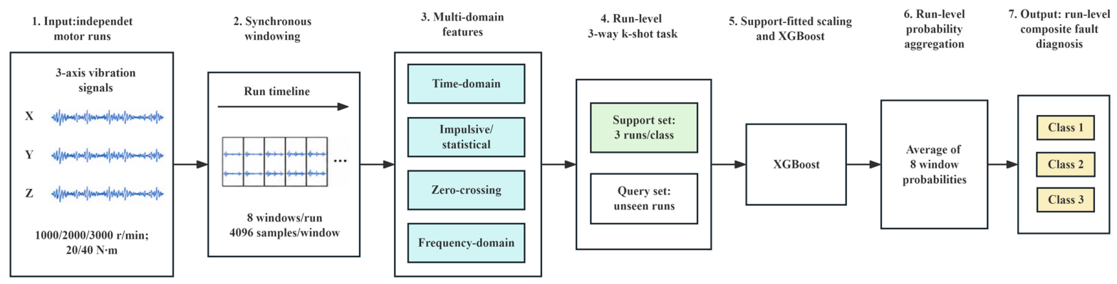
The proposed diagnostic workflow consists of seven stages: independent-run input, synchronized window construction, multidomain vibration feature extraction, run-level K-shot task construction, support-set-based feature standardization and XGBoost classification, within-run probability aggregation, and run-level diagnostic output.

After classifier training, TreeSHAP is applied separately as a post hoc feature-attribution module to analyze the contributions of the input features to the model outputs. TreeSHAP does not participate in model fitting or diagnostic prediction. The overall workflow is illustrated in Figure 1.

First, synchronized windows are extracted from the X-, Y-, and Z-axis vibration signals of each complete run according to a unified deterministic rule. Suppose that a complete run contains L sampling points, the window length is N, and the candidate-window stride is s. The number of candidate windows is:

$$\mathrm{Q}=⌊{\displaystyle \frac{\mathrm{L}-\mathrm{N}}{\mathrm{s}}}⌋+1$$

(1)

where $⌊·⌋$ denotes the floor operation.

The parameters used in this study were $L=\mathrm{1,152,000},N=4096$ and $s=2048$. Accordingly, $Q=561$ candidate windows were initially generated from each run. The candidate stride was half the window length, resulting in a 50% overlap between adjacent candidate windows.

The final number of selected windows, $\mathrm{W}=8$, was specified before evaluating the test compound fault classes. This value was used to balance coverage of the complete run, correlation among windows from the same run, and task-level computational cost. It is not interpreted as a universally optimal number of windows for all datasets.

To evaluate the sensitivity of the diagnostic results to the predefined number of selected windows, additional strict 3-shot experiments were conducted using $W\in \{4,8,16\}$. The window length $N=4096$, candidate stride $s=2048$, support and query run IDs, 48-dimensional feature definitions, and XGBoost hyperparameters were held unchanged. For each value of $W$, the windows were selected using the same deterministic equal-spacing rule in Equation (2), with identical starting positions for the three vibration axes. The predefined $W=8$ configuration remained the primary setting and was not retrospectively selected according to the sensitivity-test results.

To avoid dividing one run into a large number of highly correlated training samples while maintaining approximately uniform coverage of the entire run, $\mathrm{W}=8$ windows were selected at equal intervals from the candidate-window sequence. The candidate index and starting sampling position of the w-th selected window were defined as follows:

$${\mathrm{q}}_{\mathrm{w}}=\mathrm{r}\mathrm{o}\mathrm{u}\mathrm{n}\mathrm{d}\left[{\displaystyle \frac{\mathrm{w}(\mathrm{Q}-1)}{\mathrm{W}-1}}\right],\hspace{1em}\mathrm{w}=0,1,\dots ,\mathrm{W}-1,$$

(2)

$${\mathsf{\tau }}_{\mathrm{w}}={\mathrm{q}}_{\mathrm{w}}\mathrm{s}.$$

(3)

Under the current data configuration, the starting sampling positions of the eight selected windows were $[0,163,840,327,680,491,520,655,360,819,200,983,040,1,146,880]$.

Exactly the same starting and ending positions were used for the X-, Y-, and Z-axis vibration signals, ensuring strict synchronization of the triaxial signals at the sampling-point level. Although adjacent candidate windows overlap by 50%, the eight finally selected windows do not overlap under the fixed run length used in this study and approximately cover the complete run uniformly.

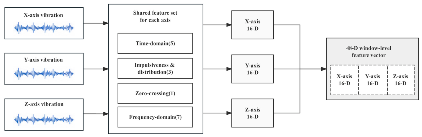
Window-level features were subsequently extracted from four domains: time-domain amplitude, impulsiveness and statistical distribution, zero-crossing characteristics, and frequency-domain structure. Sixteen features were extracted from each vibration axis, and the triaxial features were concatenated in a fixed order to form a 48-dimensional window-level feature vector.

For each few-shot task, the feature scaler was fitted using only the windows in the current support set. The standardized support features were then used to train the XGBoost classifier.

For each query run, the model first produced class probabilities for its eight windows. The probabilities were then averaged within the run to obtain the run-level class probabilities and final diagnostic result. After classifier training, TreeSHAP was used to analyze the contributions of individual input features to the raw class scores. TreeSHAP was applied only for post-training decision interpretation and did not participate in window construction, feature standardization, model fitting, or hyperparameter selection.

3.4. Multidomain Vibration Feature Extraction

Let the vibration signal within a window along one axis be expressed as follows:

$$\mathrm{x}={\left[{\mathrm{x}}_0,{\mathrm{x}}_1,\dots ,{\mathrm{x}}_{\mathrm{N}-1}\right]}^{\mathrm{T}},\mathrm{N}=4096.$$

(4)

At a sampling frequency of ${\mathrm{f}}_{\mathrm{s}}=12.8\mathrm{k}\mathrm{H}\mathrm{z}$, each window corresponds to approximately 0.32 s of vibration data. The same window boundaries are used for the X-, Y-, and Z-axis signals to maintain temporal synchronization among the triaxial vibration measurements.

Window-level features are constructed from four domains: time-domain amplitude, impulsiveness and statistical distribution, zero-crossing characteristics, and frequency-domain structure. The features extracted from each axis are summarized in

Table 4. Composition of the multidomain features extracted from each window.

Feature Category	Features per Axis	Features for Three Axes	Specific Features
Time-domain amplitude	5	15	Mean, standard deviation, root mean square, maximum absolute value, and peak-to-peak value
Impulsiveness and distribution	3	9	Crest factor, skewness, and kurtosis
Zero-crossing characteristics	1	3	Zero-crossing rate
Frequency-domain structure	7	21	Normalized spectral centroid, normalized spectral bandwidth, normalized dominant frequency, and four relative band energies
Total	16	48	Concatenated triaxial features

, and the concatenation of the triaxial features is illustrated in Figure 2.

As shown in Table 4 and Figure 2, 16 features are extracted from each vibration direction, including five time-domain amplitude features, three impulsiveness and distribution features, one zero-crossing-rate feature, and seven frequency-domain features.

The mean, population standard deviation, root mean square, maximum absolute value, and peak-to-peak value are defined as follows, respectively:

$$\mathsf{\mu }={\displaystyle \frac{1}{\mathrm{N}}}{\displaystyle \sum _{\mathrm{n}=0}^{\mathrm{N}-1}}{\mathrm{x}}_{\mathrm{n}},$$

(5)

$$\mathsf{\sigma }=\sqrt{{\displaystyle \frac{1}{\mathrm{N}}}{\displaystyle \sum _{\mathrm{n}=0}^{\mathrm{N}-1}}{({\mathrm{x}}_{\mathrm{n}}-\mathsf{\mu })}^2+\mathsf{\epsilon }},$$

(6)

$${\mathrm{x}}_{\mathrm{rms}}=\sqrt{{\displaystyle \frac{1}{\mathrm{N}}}{\displaystyle \sum _{\mathrm{n}=0}^{\mathrm{N}-1}}{\mathrm{x}}_{\mathrm{n}}^2+\mathsf{\epsilon }},$$

(7)

$${\mathrm{x}}_{\max }=\underset{0\le \mathrm{n}<\mathrm{N}}{\max }|{\mathrm{x}}_{\mathrm{n}}|,$$

(8)

$${\mathrm{x}}_{\mathrm{pp}}=\underset{0\le \mathrm{n}<\mathrm{N}}{\max }{\mathrm{x}}_{\mathrm{n}}-\underset{0\le \mathrm{n}<\mathrm{N}}{\min }{\mathrm{x}}_{\mathrm{n}}$$

(9)

where $\mathsf{\epsilon }=10^{-8}$ is a numerical-stability constant. Equation (6) uses the population standard deviation with N as the denominator. The stability term is placed inside the square root for both the standard deviation and root mean square.

The crest factor, skewness, and kurtosis are defined as follows:

$$\mathrm{CF}={\displaystyle \frac{{\mathrm{x}}_{\mathrm{m}\mathrm{a}\mathrm{x}}}{{\mathrm{x}}_{\mathrm{rms}}}},$$

(10)

$$\mathrm{Skew}={\displaystyle \frac{1}{\mathrm{N}}}{\displaystyle \sum _{\mathrm{n}=0}^{\mathrm{N}-1}}{\left({\displaystyle \frac{{\mathrm{x}}_{\mathrm{n}}-\mathsf{\mu }}{\mathsf{\sigma }}}\right)}^3,$$

(11)

$$\mathrm{Kurt}={\displaystyle \frac{1}{\mathrm{N}}}{\displaystyle \sum _{\mathrm{n}=0}^{\mathrm{N}-1}}{\left({\displaystyle \frac{{\mathrm{x}}_{\mathrm{n}}-\mathsf{\mu }}{\mathsf{\sigma }}}\right)}^4.$$

(12)

Both skewness and kurtosis are calculated using population-standardized central moments. A subtraction of 3 is not applied to the kurtosis. Therefore, the resulting feature represents ordinary kurtosis rather than excess kurtosis.

The zero-crossing rate is calculated according to changes in the sign states of adjacent sampling points. Define the negative-value indicator as ${\mathrm{b}}_{\mathrm{n}}=\mathrm{II}\left({\mathrm{x}}_{\mathrm{n}}<0\right)$, where $\mathrm{II}(\cdot )$ denotes the indicator function. The zero-crossing rate is then calculated as follows:

$$\mathrm{Z}\mathrm{C}\mathrm{R}={\displaystyle \frac{1}{\mathrm{N}-1}}{\displaystyle \sum _{\mathrm{n}=0}^{\mathrm{N}-2}}\mathrm{II}({\mathrm{b}}_{\mathrm{n}+1}\ne {\mathrm{b}}_{\mathrm{n}}).$$

(13)

where $\mathrm{II}(·)$ is the indicator function, which equals 1 when the condition is satisfied and 0 otherwise. The window signal is not demeaned before calculation, and sampling points with a value of zero are treated as nonnegative. Therefore, a change from a negative value to zero is counted as a sign-state transition.

For the frequency-domain features, a real-valued fast Fourier transform is used to obtain the one-sided spectrum. Because $N$ is even, the one-sided spectrum contains ${\mathrm{N}}_{+}={\displaystyle \frac{\mathrm{N}}{2}}+1$ nonnegative frequency positions.

The discrete spectrum and corresponding power weight at the k-th frequency position are defined as follows:

$${\mathrm{X}}_{\mathrm{k}}={\displaystyle \sum _{\mathrm{n}=0}^{\mathrm{N}-1}}{\mathrm{x}}_{\mathrm{n}}\exp \left(-\mathrm{j}{\displaystyle \frac{2\mathsf{\pi }\mathrm{k}\mathrm{n}}{\mathrm{N}}}\right),\hspace{1em}\mathrm{k}=0,1,\dots ,{\mathrm{N}}_{+}-1,$$

(14)

$${\mathrm{P}}_{\mathrm{k}}={\left|{\mathrm{X}}_{\mathrm{k}}\right|}^2,{\mathrm{P}}_0=0.$$

(15)

where $\mathrm{j}=\sqrt{-1}$. The squared magnitude of the real-valued fast Fourier transform is used as the power weight. The power corresponding to the direct-current component is set to zero to reduce the influence of signal-mean offsets on the frequency-domain statistics.

The normalized and actual frequencies corresponding to the k-th spectral position are defined as follows, respectively:

$${\nu }_k={\displaystyle \frac{k}{N_{+}-1}}={\displaystyle \frac{2k}{N}}.$$

(16)

$${\mathrm{f}}_{\mathrm{k}}={\mathsf{\nu }}_{\mathrm{k}}{\displaystyle \frac{{\mathrm{f}}_{\mathrm{s}}}{2}},$$

(17)

The stabilized total power is defined as follows:

$${\mathrm{P}}_{\mathsf{\Sigma }}={\displaystyle \sum _{\mathrm{k}=0}^{{\mathrm{N}}_{+}-1}}{\mathrm{P}}_{\mathrm{k}}+\mathsf{\epsilon }.$$

(18)

Here, ${\mathrm{v}}_{\mathrm{k}}=0$ corresponds to the direct-current frequency, whereas ${\mathrm{v}}_{\mathrm{k}}=1$ corresponds to the Nyquist frequency, ${\mathrm{f}}_{\mathrm{s}}/2=6.4\mathrm{k}\mathrm{H}\mathrm{z}$. Therefore, the normalized spectral centroid, normalized spectral bandwidth, and normalized dominant frequency used in this study are dimensionless features normalized with respect to the Nyquist frequency.

The normalized spectral centroid, normalized spectral bandwidth, and normalized dominant frequency are defined as follows, respectively:

$${\mathsf{\nu }}_{\mathrm{c}}={\displaystyle \frac{{\displaystyle {\sum }_{\mathrm{k}=0}^{{\mathrm{N}}_{+}-1}}{\mathsf{\nu }}_{\mathrm{k}}{\mathrm{P}}_{\mathrm{k}}}{{\mathrm{P}}_{\mathsf{\Sigma }}}},$$

(19)

$${\mathrm{B}}_{\mathsf{\nu }}=\sqrt{{\displaystyle \frac{{{\displaystyle {\sum }_{\mathrm{k}=0}^{{\mathrm{N}}_{+}-1}}\left({\mathsf{\nu }}_{\mathrm{k}}-{\mathsf{\nu }}_{\mathrm{c}}\right)}^2{\mathrm{P}}_{\mathrm{k}}}{{\mathrm{P}}_{\mathsf{\Sigma }}}}},$$

(20)

$${\mathrm{k}}^{\mathrm{*}}=\arg \max {\mathrm{P}}_{\mathrm{k}},0\le \mathrm{k}<{\mathrm{N}}_{+}$$

(21)

$${\mathsf{\nu }}_{\mathrm{d}}={\mathsf{\nu }}_{{\mathrm{k}}^{\mathrm{*}}}.$$

(22)

The normalized spectral centroid ${\mathsf{\nu }}_{\mathrm{c}}$ describes the central location of the spectral power along the normalized frequency axis. The normalized spectral bandwidth ${\mathrm{B}}_{\mathrm{v}}$ describes the dispersion of the spectral power around its centroid. The normalized dominant frequency ${\mathrm{v}}_{\mathrm{d}}$ corresponds to the frequency position with the maximum power.

To characterize relative energy distributions over different frequency ranges, the one-sided spectrum is approximately divided into four frequency bands. The band-boundary indices are defined as follows:

$${\mathrm{b}}_{\mathrm{j}}=⌊{\displaystyle \frac{\mathrm{j}{\mathrm{N}}_{+}}{4}}⌋,\mathrm{j}=0,1,2,3,{\mathrm{b}}_4={\mathrm{N}}_{+}.$$

(23)

The index set of the j-th frequency band is:

$${\mathcal{B}}_j=\left\{k\mid b_{j-1}\le k<b_j\right\},j=1,2,3,4.$$

(24)

The corresponding relative band energy is defined as follows:

$${\mathrm{E}}_{\mathrm{j}}={\displaystyle \frac{\sum _{\mathrm{k}\in {\mathcal{B}}_{\mathrm{j}}}{\mathrm{P}}_{\mathrm{k}}}{{\mathrm{P}}_{\mathsf{\Sigma }}}},\mathrm{j}=1,2,3,4.$$

(25)

For $\mathrm{N}=4096$, the one-sided spectrum contains ${\mathrm{N}}_{+}=2049$ frequency positions. The five boundary indices defining the four frequency bands are $[0,512,1024,1536,2049].$

The corresponding frequency ranges are approximately 0–1.6 kHz, 1.6–3.2 kHz, 3.2–4.8 kHz, and 4.8–6.4 kHz. The direct-current power in the first frequency band is set to zero according to Equation (15).

Each vibration axis produces a 16-dimensional feature vector. The features are concatenated in the fixed order of the X, Y, and Z axes to obtain the 48-dimensional window-level feature vector:

$$\mathrm{z}={\left[{\left({\mathrm{z}}^{\mathrm{X}}\right)}^{\mathrm{T}},{\left({\mathrm{z}}^{\mathrm{Y}}\right)}^{\mathrm{T}},{\left({\mathrm{z}}^{\mathrm{Z}}\right)}^{\mathrm{T}}\right]}^{\mathrm{T}}\in {\mathbb{R}}^{48}.$$

(26)

XGBoost and Random Forest use exactly the same window locations and 48-dimensional multidomain feature-extraction rules. The run-level prototypical network uses the same synchronized window locations but directly takes the standardized raw triaxial vibration signals as inputs. For all methods, query-run labels are not used for preprocessing-parameter estimation, model training, or parameter selection.

3.5. XGBoost Classification and Run-Level Probability Aggregation

XGBoost is a gradient-boosting method based on a regularized additive tree model and performs nonlinear classification by iteratively constructing decision trees [43]. Because each target task contains only a few run-ID-disjoint support runs, the XGBoost classifier is reinitialized for every 3-way K-shot task, where $\mathrm{K}\in \left\{\mathrm{1,3}\right\}$.

The classifier is fitted using only the window-level features from the support runs of the current task. Neither the query runs nor their labels participate in feature standardization, classifier training, or hyperparameter selection.

Before model fitting, a feature-wise standardizer is fitted using the support windows of the current task. Suppose that the support set contains $N_s$ window-level samples and that the raw feature vector of the i-th sample is $f_i={\left[f_{i,1},f_{i,2},\dots ,f_{i,D}\right]}^T$, where $D=48$. The number of support windows is $N_s=CKW$, where $C=3$ is the number of candidate classes, $K\in \{1,3\}$ is the number of support runs per class, and $W=8$ is the number of windows extracted from each run. Thus, $N_s=24$ for $K=1$ and $N_s=72$ for $K=3$.

The support-set mean and population variance in the d-th feature are calculated as follows, respectively:

$${\mathsf{\mu }}_{\mathrm{d}}^{\left(\mathrm{S}\right)}={\displaystyle \frac{1}{{\mathrm{N}}_{\mathrm{s}}}}{\displaystyle \sum _{\mathrm{i}=1}^{{\mathrm{N}}_{\mathrm{s}}}}{\mathrm{f}}_{\mathrm{i},\mathrm{d}},\hspace{1em}\mathrm{d}=1,2,\dots ,\mathrm{D},$$

(27)

$${\mathrm{v}}_{\mathrm{d}}^{\left(\mathrm{S}\right)}={\displaystyle \frac{1}{{\mathrm{N}}_{\mathrm{s}}}}{\displaystyle \sum _{\mathrm{i}=1}^{{\mathrm{N}}_{\mathrm{s}}}}{{(\mathrm{f}}_{\mathrm{i},\mathrm{d}}-{\mathsf{\mu }}_{\mathrm{d}}^{\left(\mathrm{S}\right)})}^2,$$

(28)

The scaling factor is defined as follows:

$${\mathrm{a}}_{\mathrm{d}}^{\left(\mathrm{S}\right)}=\left\{\begin{array}{ll}\sqrt{{\mathrm{v}}_{\mathrm{d}}^{\left(\mathrm{S}\right)}},& {\mathrm{v}}_{\mathrm{d}}^{\left(\mathrm{S}\right)}>0,\\ 1,& {\mathrm{v}}_{\mathrm{d}}^{\left(\mathrm{S}\right)}=0,\end{array}\right.$$

(29)

The standardized feature is then obtained as follows:

$${\tilde{\mathrm{f}}}_{\mathrm{i},\mathrm{d}}={\displaystyle \frac{{\mathrm{f}}_{\mathrm{i},\mathrm{d}}-{\mathsf{\mu }}_{\mathrm{d}}^{\left(\mathrm{S}\right)}}{{\mathrm{a}}_{\mathrm{d}}^{\left(\mathrm{S}\right)}}}.$$

(30)

Query windows are transformed using only ${\mathsf{\mu }}_{\mathrm{d}}^{\left(\mathrm{S}\right)}$ and ${\mathrm{a}}_{\mathrm{d}}^{\left(\mathrm{S}\right)}$, which are estimated from the support set. When the variance in a feature is zero in the support set, its scaling factor is set to 1. This treatment is consistent with the StandardScaler implementation used in this study and prevents the query data from contributing to preprocessing-parameter estimation.

XGBoost uses the multi:softprob objective and outputs the predicted probabilities of the three candidate compound fault classes for each query window. The hyperparameters were determined through preliminary experiments using the training and validation combinations and were frozen before evaluating the test compound fault classes. The final parameter settings are listed in

Table 5. Final XGBoost parameter settings.

Parameter	Setting
Objective	multi:softprob
Number of classes	3
Number of boosting rounds	250
Maximum tree depth	6
Learning rate	0.05
Row subsampling ratio	0.8
Feature subsampling ratio	0.8
Tree construction method	hist
Evaluation metric	mlogloss
Number of CPU threads	10
Random seed	Seed corresponding to the current task
Feature standardization	Standard Scaler fitted on the current support set

Note: The XGBoost parameters were determined through preliminary experiments using the training and validation combinations and were frozen before evaluating the test compound fault classes. Parameters not explicitly specified retained the default values of XGBoost 3.2.0. Neither the test combinations nor the query-run labels were used during parameter selection.

.

For the r-th query run, suppose that it contains $W=8$ windows and that ${\mathrm{p}}_{\mathrm{r},\mathrm{w},\mathrm{c}}$ denotes the predicted probability that the w-th window belongs to class $c$.

The run-level class probability is defined as follows:

$${\overline{\mathrm{p}}}_{\mathrm{r},\mathrm{c}}={\displaystyle \frac{1}{\mathrm{W}}}{\displaystyle \sum _{\mathrm{w}=1}^{\mathrm{W}}}{\mathrm{p}}_{\mathrm{r},\mathrm{w},\mathrm{c}},\mathrm{c}=1,2,\cdots \mathrm{C},$$

(31)

The final run-level predicted class is:

$${\widehat{\mathrm{y}}}_{\mathrm{r}}={\arg \underset{1\le \mathrm{c}\le \mathrm{C}}{\max }\bar{\mathrm{p}}}_{\mathrm{r},\mathrm{c}}.$$

(32)

The eight selected windows have identical lengths and are deterministically distributed to approximately cover the complete acquisition run. Because no independent window-quality or reliability information is available to justify unequal weighting, equal weighting is adopted as a simple and permutation-invariant aggregation rule. The XGBoost softmax outputs are used here as relative class-decision scores for within-run aggregation rather than being interpreted as perfectly calibrated posterior probabilities. No probability calibration using query labels is performed.

To examine whether the run-level conclusions depend strongly on this aggregation choice, two alternative strategies were additionally evaluated using exactly the same fitted XGBoost models, query runs, and query windows: majority voting over window-level predicted classes and averaging of the class-specific raw margins before selecting the run-level class. The corresponding sensitivity results are reported in Section 4.3.

3.6. TreeSHAP-Based Feature-Attribution Analysis

To examine the input-feature patterns used by XGBoost for compound-fault classification, the SHAP additive feature-attribution framework was employed [44]. The native TreeSHAP algorithm implemented for tree-based models was used to calculate post hoc feature contributions [45]. TreeSHAP was applied only after model fitting and did not participate in feature extraction, classifier training, hyperparameter selection, or diagnostic prediction.

TreeSHAP explains the class-specific raw model score before the Softmax transformation rather than the final predicted probability. For a standardized window-level feature vector $\tilde{f}$ and candidate class $c$, the raw score is expressed as follows:

$$g_c\left(\tilde{\mathbf{f}}\right)={\varphi }_{0,c}+{\displaystyle \sum _{d=1}^D}{\varphi }_{d,c}\left(\tilde{f}\right),\hspace{1em}D=48,$$

(33)

where ${\varphi }_{0,c}$ denotes the baseline raw score for class $c$, and ${\varphi }_{d,c}\left(\tilde{f}\right)$ denotes the TreeSHAP contribution of feature $d$ to that class score. A positive contribution increases the corresponding raw class score, whereas a negative contribution decreases it.

Because TreeSHAP values are expressed on class-specific raw-score scales, their absolute magnitudes are not assumed to be directly comparable across independently fitted XGBoost models or across different target classes. Therefore, the contributions were first aggregated at the run level and subsequently normalized within each independently fitted model–class pair.

Let ${\varphi }_{r,e,d,c}^{\left(e\right)}$ denote the TreeSHAP contribution of feature $d$ to the raw score of class $c$ for the w-th window of query run $r$ in the e-th fold–seed–episode evaluation unit. The run-level mean absolute contribution is defined as follows:

$$A_{r,d,c}^{\left(e\right)}={\displaystyle \frac{1}{W}}{\sum }_{w=1}^W\left|{\varphi }_{r,w,d,c}^{\left(e\right)}\right|,W=8.$$

(34)

Taking the absolute value before averaging prevents positive and negative window-level contributions from cancelling each other. Each run therefore remains the basic unit used to summarize the feature-attribution pattern.

For class-specific attribution, only query runs whose true compound-fault class is $c$ are grouped together after prediction. Let ${\mathcal{R}}_{e,c}=\left\{r\mid y_r=c\right\}$, where $y_r$ denotes the true compound-fault label of query run $r$. The class-specific mean absolute contribution within evaluation unit e is calculated as follows:

$$M_{d,c}^{\left(e\right)}={\displaystyle \frac{1}{\left|R_{e,c}\right|}}\sum _{{r\in R}_{e,c}}{\mathrm{A}}_{r,d,c}^{\left(\mathrm{e}\right)}$$

(35)

The true query labels are used only for this post hoc grouping and are not used for model fitting, hyperparameter selection, or prediction.

To reduce the influence of differences in raw-score magnitude among independently fitted models and classes, the 48-dimensional contribution vector is normalized within each model–class pair:

$$R_{d,c}^{\left(e\right)}={\displaystyle \frac{M_{d,c}^{\left(e\right)}}{{\displaystyle {\sum }_{j=1}^D}{M}_{j,c}^{\left(e\right)}+\epsilon SHAP}},D=48,ϵSHAP={10}^{-12}$$

(36)

Therefore, ${\sum }_{d=1}^D{R}_{d,c}^{\left(e\right)}\approx 1$ for each independently fitted model–class pair, and $R_{d,c}^{\left(e\right)}$ represents the relative proportion of absolute model attribution assigned to feature $d$, rather than its raw TreeSHAP magnitude.

The normalized global and class-specific feature contributions are then obtained as follows:

$$I_d^{\mathrm{g}\mathrm{l}\mathrm{o}\mathrm{b}\mathrm{a}\mathrm{l}}={\displaystyle \frac{1}{\left|\mathcal{E}\right|}}\sum _{(\mathrm{e},\mathrm{c})\in \mathsf{\epsilon }}{\mathrm{R}}_{\mathrm{d},\mathrm{c}}^{\left(\mathrm{e}\right)},$$

(37)

$$I_{d,c}^{\mathrm{c}\mathrm{l}\mathrm{a}\mathrm{s}\mathrm{s}}={\displaystyle \frac{1}{\left|{\epsilon }_c\right|}}\sum _{\mathrm{e}\in {\mathsf{\epsilon }}_{\mathrm{c}}}{\mathrm{R}}_{\mathrm{d},\mathrm{c}}^{\left(\mathrm{e}\right)},$$

(38)

where $ϵ$ denotes the set of all valid evaluation-unit/class pairs and ${ϵ}_c$ denotes the evaluation units in which class $c$ appears as a test class. Under the strict 3-shot protocol, 45 independently fitted XGBoost models and three test classes per task yield 135 model–class attribution vectors for global aggregation. Because each compound-fault class appears in one outer test fold, its class-specific attribution is averaged over 15 independently fitted models corresponding to five random seeds and three support episodes.

The resulting relative contributions are used only to compare feature-use patterns and should not be interpreted as direct evidence of physical causality. A large value of $I_d^{global}$ indicates that XGBoost consistently assigns a relatively large proportion of its absolute class-score attribution to feature $\mathrm{d}$ across repeated tasks, whereas ${\mathrm{I}}_{\mathrm{d},\mathrm{c}}^{\mathrm{c}\mathrm{l}\mathrm{a}\mathrm{s}\mathrm{s}}$ characterizes the corresponding class-specific attribution pattern for compound-fault class $\mathrm{c}$. This normalized aggregation avoids directly averaging raw TreeSHAP magnitudes across independently trained models and classes. The physical implications of the dominant feature-attribution patterns are further discussed in Section 4.7.

4. Experimental Results and Analysis

4.1. Experimental Settings and Evaluation Methods

To evaluate the proposed framework under variable operating conditions and the run-disjoint protocol, the experiments examined partitioning protocols, support-set sizes, diagnostic methods, class-level performance, feature contributions, operating-condition generalization, and computational efficiency. All methods used identical fold partitions, random seeds, candidate support runs, and query runs.

RPN employed a three-channel ResNet1D encoder containing two residual blocks, each with two one-dimensional convolutional layers, 128 output channels, and a kernel size of 5. Adaptive global average pooling followed by ${\mathcal{l}}_2$ normalization produced a 128-dimensional embedding for each window. The encoder was pretrained for up to 60 epochs using the AdamW optimizer implemented in PyTorch 2.5.1, with an initial learning rate of 0.001, a batch size of 64, and multilabel binary cross-entropy over 14 atomic fault nodes. The encoder checkpoint with the lowest validation loss on the validation combinations was retained. During target-task evaluation, the frozen window embeddings were averaged first within each run and then across support runs of the same class to construct prototypes; query runs were classified using cosine similarity.

RPN used the training combinations to pretrain its encoder, whereas Random Forest implemented in scikit-learn 1.7.2 and XGBoost 3.2.0 fitted task-specific classifiers using only the support set of each target task. Therefore, the comparison reflects different few-shot adaptation paradigms under identical target tasks rather than models trained with identical source-data budgets.

To broaden the comparison with optimization-based meta-learning approaches, standard second-order MAML [34] and ANIL were additionally implemented as controlled few-shot baselines. Both methods used a three-channel ResNet1D backbone with two residual blocks and a 128-dimensional representation. Group normalization was used instead of batch normalization to avoid task-dependent running-state leakage during functional inner-loop adaptation. For MAML, both the encoder and classification head were updated during inner-loop adaptation, whereas for ANIL only the classification head was adapted. The outer-loop parameters were trained using only the training combinations of each fold, and hyperparameters and checkpoints were selected exclusively using the corresponding validation combinations. The target test combinations were not accessed before the final evaluation. Because each outer fold contained only two validation compound-fault combinations, validation episodes were necessarily two-way, whereas meta-training and final target evaluation remained three-way.

The compared methods included the run-level prototypical network (RPN), Random Forest, full-feature XGBoost, MAML, and ANIL. RPN represents a metric-based few-shot approach using pretrained deep representations, Random Forest represents a bagging-based tree ensemble, XGBoost is the gradient-boosted tree classifier adopted in the proposed workflow, and MAML and ANIL represent optimization-based meta-learning baselines. The main procedures, input representations, prior source-training usage, and target-task adaptation strategies of the five methods are summarized in

Table 6. Main comparison methods.

Method	Input	Prior Source Training	Target-Task Adaptation
XGBoost	48-D multidomain features	No	Classifier fitted using current target support windows
Random Forest	48-D multidomain features	No	Classifier fitted using current target support windows
RPN	Raw triaxial vibration	Yes	Frozen representations + run-level prototype construction
MAML	Raw triaxial vibration	Yes	Encoder and head adapted using target support runs
ANIL	Raw triaxial vibration	Yes	Classification head adapted using target support runs

.

All five methods used identical target support and query tasks. However, their prior-data usage differed. XGBoost and Random Forest did not use a pretrained source model, whereas RPN, MAML, and ANIL used the training combinations for representation or meta learning and the validation combinations for model selection. Therefore, comparisons across these paradigms should be interpreted as practical comparisons between different few-shot adaptation strategies rather than as comparisons under identical total training-data budgets.

Three additional controlled variants were constructed to investigate the effects of correlated support windows, input representation, and classifier design under the strict three-shot setting. For Run-XGBoost, the eight 48-dimensional feature vectors belonging to each complete run were arithmetically averaged before classifier fitting, such that each support run contributed exactly one 48-dimensional training vector. Consequently, each three-way three-shot task contained only nine classifier-training samples. The feature standardizer was fitted using these nine support-run vectors, and the same frozen XGBoost hyperparameters as in the principal experiments were retained without additional tuning.

For Feature-Proto, exactly the same standardized 48-dimensional run-mean vectors as those used by Run-XGBoost were employed. A prototype was constructed by averaging the three support-run vectors belonging to each target class, and query runs were classified using cosine similarity. Thus, Run-XGBoost and Feature-Proto differed primarily in classifier design while sharing the same handcrafted run-level representation.

For Embedding-XGBoost, the validation-selected and frozen RPN encoder was reused without retraining. The eight 128-dimensional window embeddings of each run were averaged to obtain the same run-level representation used by RPN. XGBoost was then fitted using the target support-run embeddings with the frozen XGBoost hyperparameters. Therefore, RPN and Embedding-XGBoost shared exactly the same learned run-level representation but used different classifiers. No query labels were used for preprocessing, fitting, or parameter selection in any of these controlled variants.

Random Forest consisted of 500 decision trees, with n_jobs = 10 and a random seed corresponding to the current task. All remaining parameters retained the default settings of scikit-learn 1.7.2. Both XGBoost and Random Forest used 10 CPU threads in the computational-efficiency experiments.

As shown in

Table 7. Experimental environment and repeated-evaluation settings.

Item	Configuration
Python	3.10.20
XGBoost	3.2.0
NumPy/pandas	2.2.6/2.3.3
scikit-learn	1.7.2
PyTorch/CUDA	2.5.1/12.1
CPU	Intel processor with 14 physical cores and 20 logical cores
GPU	NVIDIA GeForce RTX 4060 Laptop GPU, 8 GiB
Memory	15.8 GiB
Number of folds	3
Random seeds	42, 52, 62, 72, and 82
Number of episodes per seed	3
Number of repeated task instances	45

, each method was evaluated using three folds, five random seeds, and three episodes for each seed, resulting in 45 repeated task instances. Task-level means and standard deviations were used to describe the performance distributions across different target-class combinations and support tasks. However, these task instances were not treated as mutually independent physical experimental samples.

For statistical inference regarding the difference between the one-shot and three-shot settings, the predicted probabilities of the same query run were first averaged across different episodes. Each unique run ID was then treated as the paired statistical unit. A class-stratified bootstrap procedure with 10,000 resamples was conducted according to the true compound fault classes, and 95% confidence intervals were reported.

An analogous protocol-specific paired bootstrap was performed for the matched Run-disjoint versus Window-mixed comparison. Because the same physical query run could appear in multiple support episodes, repeated class-probability predictions were first averaged separately within each protocol and unique query-run ID. This produced one aggregated prediction for each physical query run under each protocol. A class-stratified paired bootstrap with 10,000 resamples was then performed over the unique run IDs, with exactly the same resampled run IDs used for both protocols in each bootstrap replicate. The bootstrap statistic was defined as ${\mathsf{\Delta }}_{\mathrm{l}\mathrm{e}\mathrm{a}\mathrm{k}}={\mathrm{M}\mathrm{a}\mathrm{c}\mathrm{r}\mathrm{o}\mathrm{F}1}_{\mathrm{W}\mathrm{i}\mathrm{n}\mathrm{d}\mathrm{o}\mathrm{w}-\mathrm{m}\mathrm{i}\mathrm{x}\mathrm{e}\mathrm{d}}-{\mathrm{M}\mathrm{a}\mathrm{c}\mathrm{r}\mathrm{o}\mathrm{F}1}_{\mathrm{R}\mathrm{u}\mathrm{n}-\mathrm{d}\mathrm{i}\mathrm{s}\mathrm{j}\mathrm{o}\mathrm{i}\mathrm{n}\mathrm{t}}.$ The 2.5th and 97.5th percentiles of the bootstrap distribution were used to construct the 95% confidence interval. The task-level mean difference and the unique-run bootstrap estimate are reported separately because they use different statistical units.

The diagnostic results were evaluated at both the compound fault class level and the atomic fault component level. For class $\mathrm{c}$, precision, recall, and F1-score are defined as follows, respectively:

$$\mathrm{P}\mathrm{r}\mathrm{e}\mathrm{c}\mathrm{i}\mathrm{s}\mathrm{i}\mathrm{o}{\mathrm{n}}_{\mathrm{c}}={\displaystyle \frac{\mathrm{T}{\mathrm{P}}_{\mathrm{c}}}{\mathrm{T}{\mathrm{P}}_{\mathrm{c}}+\mathrm{F}{\mathrm{P}}_{\mathrm{c}}}},$$

(39)

$${\mathrm{R}\mathrm{e}\mathrm{c}\mathrm{a}\mathrm{l}\mathrm{l}}_{\mathrm{c}}={\displaystyle \frac{\mathrm{T}{\mathrm{P}}_{\mathrm{c}}}{\mathrm{T}{\mathrm{P}}_{\mathrm{c}}+\mathrm{F}{\mathrm{N}}_{\mathrm{c}}}},$$

(40)

$$\mathrm{F}{1}_{\mathrm{c}}={\displaystyle \frac{2\mathrm{P}\mathrm{r}\mathrm{e}\mathrm{c}\mathrm{i}\mathrm{s}\mathrm{i}\mathrm{o}{\mathrm{n}}_{\mathrm{c}}\mathrm{R}\mathrm{e}\mathrm{c}\mathrm{a}\mathrm{l}{\mathrm{l}}_{\mathrm{c}}}{\mathrm{P}\mathrm{r}\mathrm{e}\mathrm{c}\mathrm{i}\mathrm{s}\mathrm{i}\mathrm{o}{\mathrm{n}}_{\mathrm{c}}+\mathrm{R}\mathrm{e}\mathrm{c}\mathrm{a}\mathrm{l}{\mathrm{l}}_{\mathrm{c}}}}.$$

(41)

where $\mathrm{T}{\mathrm{P}}_{\mathrm{c}}$,$\mathrm{F}{\mathrm{P}}_{\mathrm{c}}$, and $\mathrm{F}{\mathrm{N}}_{\mathrm{c}}$ denote the numbers of true-positive, false-positive, and false-negative predictions for class $\mathrm{c}$, respectively.

Macro-F1 and run-level accuracy are defined as follows, respectively:

$$\mathrm{M}\mathrm{a}\mathrm{c}\mathrm{r}\mathrm{o}-\mathrm{F}1={\displaystyle \frac{1}{\mathrm{C}}}{\displaystyle \sum _{\mathrm{c}=1}^{\mathrm{C}}}\mathrm{F}{1}_{\mathrm{c}},$$

(42)

$${Acc}_{run}={\displaystyle \frac{1}{N_q}}{\displaystyle \sum _{r=1}^{N_q}}\mathrm{II}({\widehat{\mathrm{y}}}_{\mathrm{r}}={\mathrm{y}}_{\mathrm{r}})$$

(43)

where $\mathrm{C}=3$ is the number of candidate compound fault classes in the current task, ${\mathrm{N}}_{\mathrm{q}}$ is the number of query runs, and ${\mathrm{y}}_{\mathrm{r}}$ and ${\widehat{\mathrm{y}}}_{\mathrm{r}}$ are the true compound fault class and run-level predicted class of the r-th query run, respectively.

To provide an auxiliary evaluation of the compound-fault predictions from the perspective of their constituent fault components, the Present-Component Macro-F1, abbreviated as PC-Macro-F1, was employed.

Let the set of atomic fault components present in the test set of the e-th evaluation unit be ${\mathcal{A}}_e=\left\{a\mid {\sum }_{r=1}^{N_q}{y}_{r,a}>0\right\}$, where $y_{r,a}$ indicates whether the r-th query run contains atomic fault component $a$. PC-Macro-F1 is then defined as follows:

$${\mathrm{P}\mathrm{C}-\mathrm{M}\mathrm{a}\mathrm{c}\mathrm{r}\mathrm{o}-\mathrm{F}1}^{\left(\mathrm{e}\right)}={\displaystyle \frac{1}{\left|{\mathcal{A}}_{\mathrm{e}}\right|}}\sum _{\mathrm{a}\in {\mathcal{A}}_{\mathrm{e}}}\mathrm{F}{1}_{\mathrm{a}}^{\left(\mathrm{e}\right)}.$$

(44)

where $\left|{\mathcal{A}}_e\right|$ denotes the number of atomic fault components present in the current test set.

The true and predicted compound fault classes of each query run were first converted into binary atomic fault component vectors according to the predefined mapping between compound faults and atomic components. For each fold-seed-episode evaluation unit, only atomic fault components with at least one positive sample in the current test set were retained. The binary F1-score was calculated separately for each of these present components and then macro-averaged.

The test sets of Fold A, Fold B, and Fold C contained five, four, and five present atomic fault components, respectively. Across the three folds, six distinct atomic fault components were covered: severe bearing inner-race fault, severe bearing outer-race fault, broken rotor bar, dynamic eccentricity, severe static eccentricity, and severe winding fault. This metric was obtained by mapping run-level compound-fault class predictions to atomic component labels. It does not indicate that an additional independent multilabel atomic-fault classifier was trained.

4.2. Comparison Between the Run-Disjoint and Window-Mixed Protocols

To directly verify the necessity of run-level data separation, a matched-query partitioning-protocol comparison was designed. The Run-disjoint and Window-mixed protocols used exactly the same 27 query run IDs, 144 query windows, and 24 support windows per class.

Each class initially contained nine query runs and 72 candidate query windows, with eight windows extracted from each run. For the matched protocol comparison, 24 windows per class were selected according to the same predefined allocation rule for support-set construction, leaving 48 query windows per class and 144 query windows in total. Both protocols used exactly these 144 query windows. Under the run-disjoint protocol, the support windows were obtained from separate support-run IDs, whereas under the window-mixed protocol, the support windows were obtained from runs that also contributed retained query windows. Run-level probabilities were calculated by averaging all retained query-window probabilities belonging to each query run.

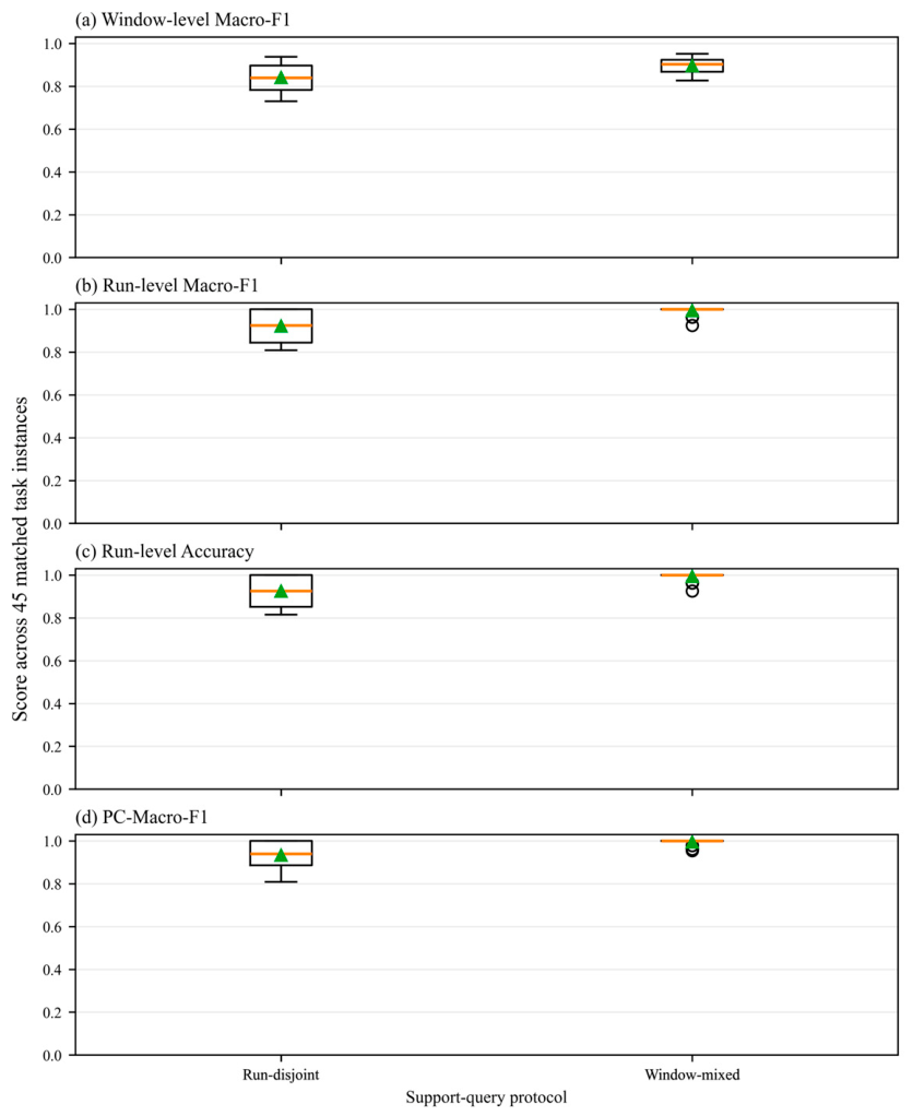
The only difference between the protocols was whether the support windows were allowed to originate from query runs. Under the run-disjoint protocol, the support and query run IDs were completely nonoverlapping. Under the window-mixed protocol, different windows from the same run could be assigned to the support and query sets. The results are presented in

Table 8. Diagnostic performance under the run-disjoint and window-mixed protocols using identical query runs and query windows.

Protocol	Window Macro-F1	Run Macro-F1	Run Accuracy	PC-Macro-F1
Run-disjoint	0.8411 ± 0.0608	0.9212 ± 0.0691	0.9243 ± 0.0658	0.9333 ± 0.0600
Window-mixed	0.8960 ± 0.0343	0.9934 ± 0.0163	0.9934 ± 0.0162	0.9945 ± 0.0132

Note: The two protocols used exactly the same 27 query run IDs, 144 query windows, and 24 support windows per class. The run-disjoint protocol required complete separation between the support-run and query-run IDs, whereas the window-mixed protocol allowed support windows to originate from query runs. The means and standard deviations were calculated over 45 matched task instances.

and Figure 3.

As shown in Table 8, the window-mixed protocol increased the task-level mean window-level Macro-F1, run-level Macro-F1, run-level accuracy, and PC-Macro-F1 by 0.0549, 0.0722, 0.0691, and 0.0612, respectively. Because the query runs, query windows, and support-window budget were held fixed, these task-level results show that allowing support windows to originate from query runs can produce optimistic estimates under particular few-shot support-task realizations.

The 0.0722 value represents the difference between the mean run-level Macro-F1 values across the 45 matched support-task instances and should not be interpreted as an effect size based on 45 independent physical experiments. An additional paired bootstrap analysis therefore treated the unique query-run ID as the statistical unit. After repeated class-probability predictions were averaged separately within each protocol and unique run, 108 unique physical query runs remained. The aggregated run-disjoint and window-mixed Macro-F1 values were 0.9907 and 1.0000, respectively, corresponding to a unique-run difference of 0.0093. The 10,000-replicate class-stratified paired bootstrap yielded a 95% percentile confidence interval of [0.0000, 0.0282].

The difference between the task-level estimate and the unique-run estimate indicates that the apparent magnitude of the leakage-related performance difference depends strongly on the statistical unit and on how repeated support-task realizations are aggregated. Therefore, the 0.0722 difference is interpreted as descriptive task-level inflation, whereas the unique-run bootstrap provides the physical-run-level statistical assessment. Because the lower percentile bound of the 95% confidence interval was 0.0000, the unique-run result is not interpreted as evidence of a strictly positive effect at the 95% confidence level. Nevertheless, strict run-ID separation remains necessary to prevent the same physical acquisition from contributing to both support and query sets by construction.

4.3. Comparison of Different Support-Set Sizes and Diagnostic Methods

Table 9. Diagnostic performance of different methods under the strict common-query protocol.

Method	Shot	Macro-F1	Run-Level Accuracy	PC-Macro-F1
XGBoost	1	0.6414 ± 0.1866	0.6527 ± 0.1778	0.6862 ± 0.1760
XGBoost	3	0.9263 ± 0.0657	0.9292 ± 0.0621	0.9360 ± 0.0597
Random Forest	1	0.6358 ± 0.1521	0.6543 ± 0.1381	0.6841 ± 0.1539
Random Forest	3	0.9167 ± 0.0775	0.9202 ± 0.0741	0.9369 ± 0.0634
RPN	1	0.8226 ± 0.1890	0.8321 ± 0.1753	0.8537 ± 0.1597
RPN	3	0.9100 ± 0.1238	0.9128 ± 0.1193	0.9241 ± 0.1039
MAML	1	0.2785 ± 0.1233	0.3597 ± 0.1222	0.3963 ± 0.1597
MAML	3	0.2679 ± 0.1191	0.3490 ± 0.1196	0.3812 ± 0.1614
ANIL	1	0.3024 ± 0.1494	0.4255 ± 0.1073	0.4061 ± 0.1952
ANIL	3	0.3361 ± 0.1915	0.4477 ± 0.1432	0.4260 ± 0.2204

Note: Three candidate support runs were first fixed for each class. The 3-shot setting used all three candidate runs, whereas the 1-shot setting used only one candidate run. The other two candidate runs were excluded from the query set. Therefore, the two shot settings used exactly the same query run IDs. The means and standard deviations were calculated over 45 repeated task instances. These 45 task instances represent repeated support-set realizations rather than 45 independent physical experiments; unique-run paired-bootstrap inference is reported in the accompanying text.

compares the five diagnostic methods under identical target support and query tasks. Under the highly restrictive one-shot setting, RPN achieved the highest Macro-F1, run-level accuracy, and PC-Macro-F1, indicating the benefit of a pretrained metric representation when only one independently labeled support run is available for each target class. With three support runs per class, the predefined XGBoost workflow achieved a Macro-F1 of 0.9263 and a run-level accuracy of 0.9292, while Random Forest obtained a slightly higher PC-Macro-F1 of 0.9369.

The controlled MAML and ANIL baselines achieved lower target-task performance under the present outer split. These results should not be interpreted as general evidence that optimization-based meta-learning is inferior for machinery fault diagnosis. In each fold, only four compound-fault combinations were available for meta-training and two for validation, providing limited source-task diversity for learning a transferable meta-initialization. The comparison therefore highlights the dependence of few-shot performance on both the adaptation paradigm and the diversity of available source tasks.

The unique-run-level stratified bootstrap analysis further showed Macro-F1 gains of 0.2716 for XGBoost and 0.2721 for Random Forest, with 95% confidence intervals of [0.2006, 0.3527] and [0.2016, 0.3580], respectively. The corresponding change for RPN was 0.0120, with a confidence interval of [−0.0274, 0.0555], which is consistent with its already strong performance under the 1-shot setting. Overall, the two tree-based classifiers obtained the clearest benefits from the additional run-disjoint support runs.

As shown in

Table 10. Sensitivity of run-level diagnostic performance to within-run aggregation rules.

Shot	Aggregation Rule	Macro-F1	Run-Level Accuracy	PC-Macro-F1
1	Mean probability	0.6414 ± 0.1866	0.6527 ± 0.1778	0.6862 ± 0.1760
1	Majority voting	0.6429 ± 0.1817	0.6535 ± 0.1732	0.6806 ± 0.1720
1	Mean raw margin	0.6470 ± 0.1909	0.6560 ± 0.1865	0.6906 ± 0.1786
3	Mean probability	0.9263 ± 0.0657	0.9292 ± 0.0621	0.9360 ± 0.0597
3	Majority voting	0.9373 ± 0.0697	0.9399 ± 0.0662	0.9464 ± 0.0620
3	Mean raw margin	0.9245 ± 0.0628	0.9276 ± 0.0591	0.9326 ± 0.0576

, the three aggregation strategies produced broadly similar run-level performance. Under the 3-shot setting, majority voting achieved the highest mean Macro-F1 of 0.9373, compared with 0.9263 for the predefined mean-probability rule and 0.9245 for raw-margin averaging. Nevertheless, only 2.22% of the 3-shot query-run predictions differed across at least two aggregation rules, and the disagreement between mean probability and majority voting was 1.32%. These results indicate that the principal run-level diagnostic conclusions are not strongly dependent on the specific aggregation rule. Mean-probability aggregation is retained in the principal experiments because it was specified before the sensitivity analysis and preserves the complete class-score information from all windows. No query-label calibration was used by any aggregation rule.

4.4. Window-Count Sensitivity and Controlled Run-Level Comparisons

Table 11. Sensitivity of XGBoost performance to the number of uniformly selected windows per run under the strict 3-shot protocol.

W	Macro-F1	Run-Level Accuracy	PC-Macro-F1	Prediction Disagreement vs. W = 8
4	0.8595 ± 0.0837	0.8617 ± 0.0833	0.8761 ± 0.0736	0.0872
8	0.9263 ± 0.0657	0.9292 ± 0.0621	0.9360 ± 0.0597	—
16	0.9743 ± 0.0354	0.9745 ± 0.0352	0.9767 ± 0.0327	0.0683

shows that diagnostic performance is sensitive to the number of local windows retained from each run. Increasing W from 4 to 8 improved the mean Macro-F1 from 0.8595 to 0.9263, and increasing W to 16 further improved it to 0.9743. Therefore, the sensitivity analysis does not indicate that W = 8 is universally optimal or that the classifier is invariant to window count. Instead, denser temporal sampling provides additional local observations of within-run vibration variability. The predefined W = 8 setting is retained in the principal experiments because it was fixed before evaluation and represents a moderate sampling budget rather than a retrospectively selected optimum. Importantly, changing W does not change the definition of a shot: one complete independently acquired run remains one shot for W = 4, 8, and 16.

The controlled comparison of run-level representation and classifier design under the strict 3-shot protocol is summarized in

Table 12. Controlled comparison of run-level representation and classifier design under the strict 3-shot protocol.

Method	Representation/Unit	Classifier/Source Pretraining	Macro-F1	Run Acc.	PC-Macro-F1
Original Window-XGBoost	48-D handcrafted/window	XGB/No	0.9263 ± 0.0657	0.9292 ± 0.0621	0.9360 ± 0.0597
Run-XGBoost	48-D run mean/run	XGB/No	0.6287 ± 0.1226	0.6370 ± 0.1165	0.6727 ± 0.1182
Feature-Proto	48-D run mean/run	Cosine prototype/No	0.6467 ± 0.1203	0.6584 ± 0.1155	0.6898 ± 0.1076
Embedding-XGBoost	Frozen RPN 128-D/run	XGB/Yes	0.8715 ± 0.1081	0.8749 ± 0.1042	0.8848 ± 0.1000
RPN	Frozen RPN 128-D/run	Cosine prototype/Yes	0.9100 ± 0.1238	0.9128 ± 0.1193	0.9241 ± 0.1039

.

The Run-XGBoost control evaluates the effect of collapsing the correlated local observations within each labeled support run before classifier fitting. In this variant, each complete support run contributed only one 48-dimensional run-mean feature vector; so, a three-way three-shot task contained exactly nine classifier-training samples. This aggregation reduced the mean Macro-F1 from 0.9263 for the original Window-XGBoost workflow to 0.6287, and the two variants disagreed on 34.73% of the repeated query-run predictions. This result indicates that retaining multiple local windows preserves information about within-run vibration variability that is largely lost when the handcrafted features are collapsed to a single arithmetic mean vector before classification. It does not alter the physical definition of a shot: the run remains the independently labeled support and statistical unit, while its windows are treated as correlated local observations used to characterize that run. Moreover, each support run contributes exactly the same predefined number W of windows to Window-XGBoost; so, the relative sample multiplicity of the support runs is equal by construction.

The same-representation comparisons further separate classifier effects from representation effects. When the same 48-dimensional handcrafted run-mean representation was used, Feature-Proto achieved a Macro-F1 of 0.6467, compared with 0.6287 for Run-XGBoost. When the same frozen 128-dimensional RPN run embeddings were used, the cosine-prototype classifier achieved 0.9100, compared with 0.8715 for Embedding-XGBoost. Thus, classifier design affects performance even when the representation is held fixed. The learned RPN representation also produced substantially higher performance than the handcrafted run-mean representation. However, this difference should not be interpreted as a pure representation-only effect because the RPN encoder was pretrained using the training combinations, whereas the handcrafted features required no source-model training. The controlled experiments therefore clarify the respective roles of classifier design and representation/prior learning without claiming identical total training-data budgets.

4.5. Fold-Level and Class-Level Diagnostic Results

To analyze the model performance across different target compound fault combinations,

Table 13. Three-shot diagnostic performance of XGBoost in different test folds.

Fold	Test Compound Faults	Macro-F1	Run-Level Accuracy	PC-Macro-F1
Fold A	BBI, SEO, and WI	0.9181 ± 0.0572	0.9210 ± 0.0539	0.9304 ± 0.0619
Fold B	BOI, DEI, and WO	0.9800 ± 0.0302	0.9802 ± 0.0298	0.9776 ± 0.0339
Fold C	BBO, DEO, and SEI	0.8807 ± 0.0587	0.8864 ± 0.0549	0.9001 ± 0.0494

presents the diagnostic results of full-feature XGBoost for the three test folds.

All three folds achieved a mean Macro-F1 above 0.88, and Fold B reached 0.9800, indicating consistently high run-level performance across different target-class combinations.

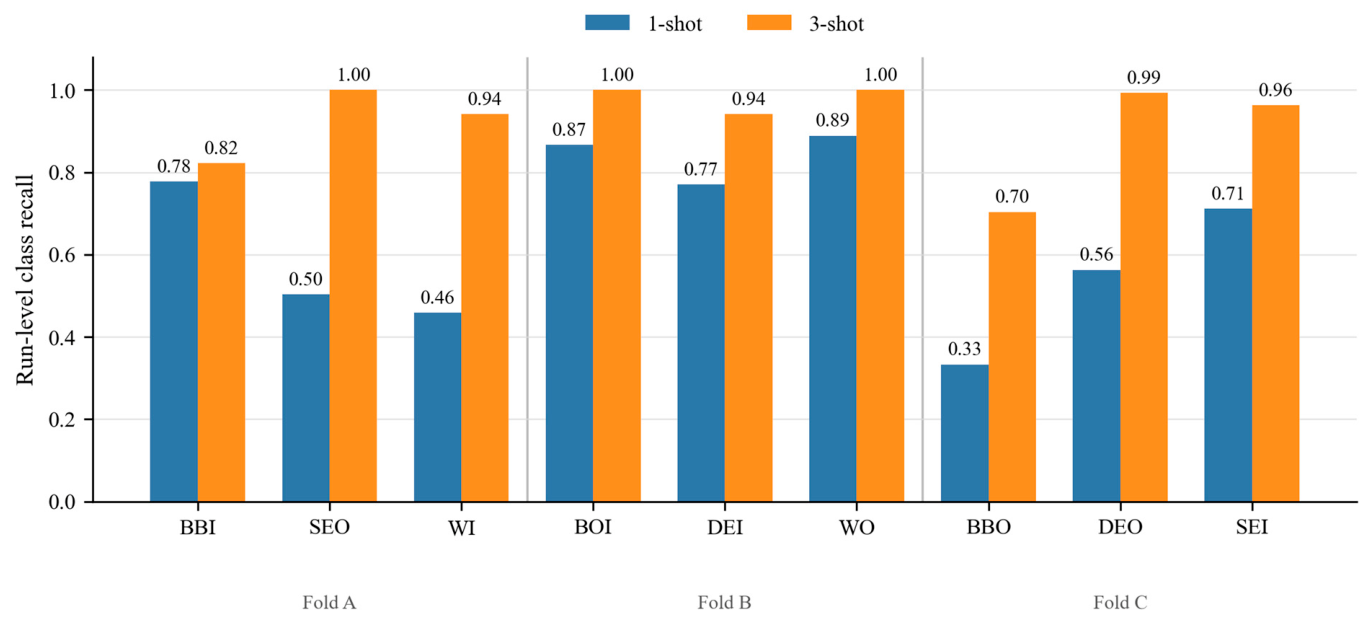
As shown in Figure 4, increasing the number of support runs from one to three improved the recall of all nine compound-fault classes. Under the 3-shot setting, seven classes achieved recall values of at least 0.94; SEO, BOI, and WO reached 1.00, while DEO and SEI reached 0.99 and 0.96, respectively. Particularly large gains were observed for SEO, WI, BBO, and DEO. Although BBO improved from approximately 0.33 to 0.70, it remained the most challenging class, followed by BBI with a recall of approximately 0.82. Overall, the results demonstrate that additional run-disjoint support runs improved class-level diagnostic performance across all target fault combinations.

Because Figure 4 presents only class-level recall, no conclusion regarding specific misclassification directions is drawn from this figure.

4.6. Multidomain Feature Ablation Results

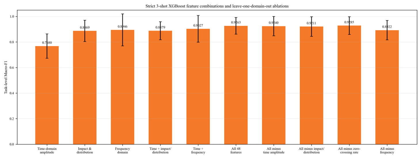
To investigate the effects of different feature domains on compound fault diagnosis, ablation experiments were performed using different feature combinations while maintaining identical fold partitions, support tasks, query runs, and XGBoost parameters. The results are presented in

Table 14. Diagnostic performance of different feature settings under the strict 3-shot protocol.

Feature Setting	Macro-F1	Run-Level Accuracy	PC-Macro-F1
Time-domain amplitude	0.7680 ± 0.0953	0.7728 ± 0.0879	0.8003 ± 0.0914
Impulsiveness and distribution	0.8869 ± 0.0834	0.8889 ± 0.0823	0.9106 ± 0.0728
Frequency-domain features	0.8946 ± 0.1253	0.8947 ± 0.1276	0.9123 ± 0.1134
Time domain + impulsiveness and distribution	0.8879 ± 0.0703	0.8889 ± 0.0707	0.9113 ± 0.0658
Time domain + frequency domain	0.9027 ± 0.1045	0.9045 ± 0.1049	0.9217 ± 0.0867
All 48 features	0.9263 ± 0.0657	0.9292 ± 0.0621	0.9360 ± 0.0597
Full features minus time-domain amplitude	0.9240 ± 0.0756	0.9267 ± 0.0726	0.9319 ± 0.0715
Full features minus impulsiveness and distribution	0.9211 ± 0.0766	0.9243 ± 0.0732	0.9313 ± 0.0687
Full features minus zero-crossing rate	0.9175 ± 0.0692	0.9109 ± 0.0665	0.9299 ± 0.0616
Full features minus frequency-domain structure	0.8922 ± 0.0759	0.8930 ± 0.0762	0.9072 ± 0.0746

Note: All feature settings used identical fold partitions, support runs, query runs, window positions, and XGBoost parameters. The means and standard deviations were calculated over 45 repeated task instances.

and Figure 5.

Figure 5 visualizes all feature settings reported in Table 14, including the single-domain, combined-domain, full-feature, and leave-one-domain-out configurations.

Time-domain amplitude features alone provided a baseline Macro-F1 of 0.7680. The impulsiveness and distribution features and the frequency-domain features increased the Macro-F1 to 0.8869 and 0.8946, respectively, demonstrating their strong discriminative value. Combining the time-domain and frequency-domain features further improved the Macro-F1 to 0.9027.

The complete 48-dimensional feature set achieved the highest Macro-F1 of 0.9263. Among the individual domains, frequency-domain and impulsiveness/distribution features yielded the strongest performance, whereas removing the frequency-domain group caused the largest decrease of 0.0341. Removing the other feature groups produced smaller but consistent reductions, demonstrating that the final performance resulted from complementary information across multiple vibration domains.

4.7. TreeSHAP-Based Feature-Attribution Results

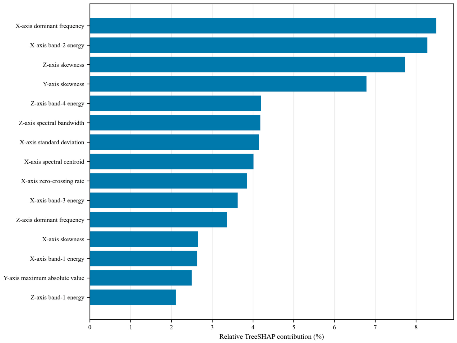
To investigate the decision basis of full-feature XGBoost, the TreeSHAP contributions obtained across different folds, random seeds, and support tasks were first aggregated. The global feature-contribution distribution is presented in Figure 6.

As shown in Figure 6, the X-axis normalized dominant frequency exhibited the largest global relative TreeSHAP contribution (8.49%), followed by the X-axis second-band relative energy (8.28%), Z-axis skewness (7.73%), and Y-axis skewness (6.78%). The Top 15 features covered all four feature categories, including time-domain amplitude, impulsiveness and statistical distribution, zero-crossing characteristics, and frequency-domain structure. Frequency-position and band-energy descriptors occupied several of the highest-ranking positions, indicating that spectral-location and energy-distribution information played an important role in the classifier decisions. Distribution-related features, particularly skewness, also contributed strongly across multiple vibration directions.

As a robustness check, the normalized global ranking was compared with the original ranking obtained from unnormalized mean absolute TreeSHAP values. The two rankings showed a Spearmans’ rank correlation of 0.9959, with complete Top 10 and Top 15 feature-set overlap. Thus, normalization altered several relative ranks and magnitudes but did not materially change the set of dominant features identified by the analysis.

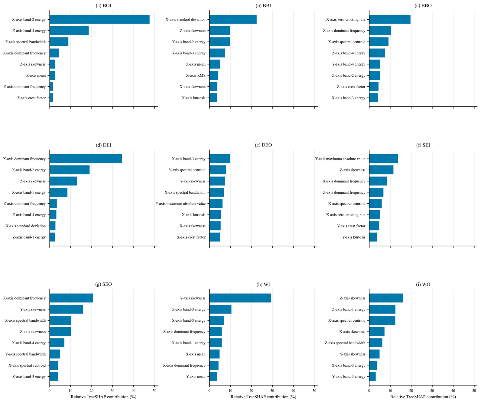
The class-specific TreeSHAP contributions for the nine compound fault classes under the strict three-shot protocol are shown in Figure 7.

Figure 7 reveals distinct class-specific feature-attribution patterns. BOI relies strongly on X-axis second-band energy, whereas DEI and SEO assign the largest relative contribution to the X-axis normalized dominant frequency. BBO is most strongly associated with the X-axis zero-crossing rate, while WI is dominated by Y-axis skewness. Other classes show broader combinations of spectral, distribution-related, and multiaxis features. These class-dependent patterns indicate that the classifier distinguishes different compound-fault combinations using different mixtures of vibration characteristics rather than a single universally dominant feature.

From a vibration-physics perspective, the dominant attribution patterns are qualitatively consistent with different properties of motor vibration signals. Spectral-position and band-energy features characterize changes in periodic or modulated vibration energy, whereas skewness and other distribution-related features reflect waveform asymmetry and impulsive behavior. Zero-crossing rate further characterizes changes in oscillatory sign-transition behavior. These signal properties can be affected by bearing, rotor, eccentricity, and winding-related disturbances. However, the present 48-dimensional representation does not explicitly encode shaft-order components or analytical bearing characteristic frequencies. Therefore, the TreeSHAP results are interpreted as feature-attribution-based evidence of the signal characteristics used by the classifier rather than as direct identification of individual physical fault mechanisms.

4.8. Diagnostic Results Under Strict Operating-Condition Separation

The main experiments evaluated few-shot diagnostic performance when the task data covered multiple speeds and loads. They did not require the support and query sets to be completely separated along a particular operating-condition dimension.

All controlled operating-condition experiments retained the run-disjoint three-way 3-shot setting. For each target class, the support runs were selected exclusively from the designated support condition, while the query runs were collected from the completely nonoverlapping target condition. Feature standardization was fitted using only the support runs, and the classifier settings were identical to those used in the main experiments. The reported results were calculated over 45 repeated task instances.

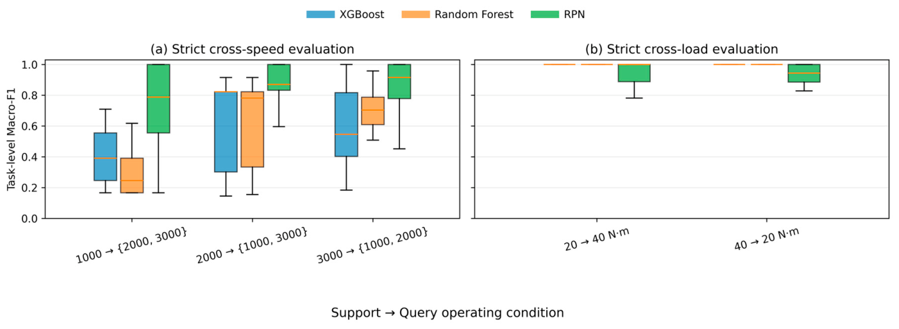
To further investigate the applicability boundaries of XGBoost, Random Forest, and RPN, three cross-speed tasks were constructed in which the support and query speeds were completely nonoverlapping. Two cross-load tasks were also constructed in which the support and query loads were completely nonoverlapping. The results are presented in

Table 15. Macro-F1 in controlled cross-speed and cross-load tasks.

Operating-Condition Dimension	Support-to-Query Direction	XGBoost	Random Forest	RPN
Speed	1000 → {2000, 3000} r/min	0.4067 ± 0.1713	0.2952 ± 0.1633	0.7346 ± 0.2794
Speed	2000 → {1000, 3000} r/min	0.6238 ± 0.2643	0.6443 ± 0.2529	0.8796 ± 0.1200
Speed	3000 → {1000, 2000} r/min	0.5667 ± 0.2820	0.6997 ± 0.1249	0.8572 ± 0.1744
Load	20 → 40 N·m	1.0000 ± 0.0000	0.9975 ± 0.0117	0.9165 ± 0.1311
Load	40 → 20 N·m	0.9836 ± 0.0356	0.9950 ± 0.0161	0.9349 ± 0.0748

and Figure 8.

In the two strict cross-load tasks, XGBoost achieved Macro-F1 values of 1.0000 and 0.9836 for the 20 → 40 N·m and 40 → 20 N·m directions, respectively. Random Forest achieved similarly high values of 0.9975 and 0.9950. These results demonstrate that the multidomain vibration features maintained stable diagnostic performance across the investigated load changes.

In the strict cross-speed tasks, RPN achieved the highest mean Macro-F1 in all three directions. XGBoost obtained Macro-F1 values of 0.4067, 0.6238, and 0.5667, with its best result observed when the support runs were collected at 2000 r/min. The contrast between the cross-load and cross-speed results suggests that the fixed-frequency features are more strongly affected by rotational-frequency shifts than by the load variations represented in the dataset. This finding motivates the future incorporation of order-domain or rotational-speed-normalized spectral features.

Accordingly, the present results should not be interpreted as evidence of general cross-speed robustness. The variable-condition experiments primarily demonstrate diagnosis when multiple operating conditions are represented within the few-shot tasks and under the investigated cross-load transfers, whereas strict cross-speed generalization remains a limitation of the current fixed-frequency representation.

4.9. Computational Efficiency and Deployment Overhead

To evaluate task-level updating and deployment overhead when only a few newly labeled runs are available, the support-set fitting or adaptation time, inference time for a single query run, and model size were measured under a fixed 3-shot task. The results are presented in

Table 16. Classifier-side adaptation and cached-representation inference costs under a fixed 3-shot task.

Method	Support-Set Fitting/Adaptation Time (s)	Classification Time per Run After Representation Caching (s)	Model Size (MB)
XGBoost	0.4385	0.007222	0.575
Random Forest	0.8150	0.093145	0.788
RPN	0.0859 *	0.013267 *	1.503

Note: Values marked with an asterisk include only class-prototype construction and run-level classification after the neural embeddings have been cached. They exclude encoder training and the forward computation required to transform raw vibration signals into neural embeddings. XGBoost and Random Forest used cached 48-dimensional handcrafted features for support-set fitting and single-run inference. Therefore, the RPN timing results cannot be directly compared with those of the two tree-based models as end-to-end computational costs.

.

Under the cached-feature timing setting, XGBoost required 0.4385 s for support-set fitting, 0.007222 s for single-run classification, and 0.575 MB for model storage. Compared with Random Forest, these values correspond to reductions of approximately 46.2%, 92.2%, and 27.0%, respectively. Together with its competitive performance under the predefined strict 3-shot protocol, these results demonstrate a favorable balance between diagnostic performance and classifier-side computational overhead.

RPN required only 0.0859 s for class-prototype construction after neural embeddings had been cached. Because this timing excludes encoder training and raw-signal embedding extraction, it represents adaptation-side rather than end-to-end computational cost.

5. Discussion

The central methodological implication of this study is that the shot definition should reflect the number of independently labeled acquisition runs rather than the number of extracted windows. Across the 45 matched support-task realizations, Window-mixed partitioning increased the mean run-level Macro-F1 by 0.0722 while the query runs, query windows, and support-window budget were held fixed. However, the 45 tasks are repeated support-set realizations rather than independent physical experiments. After repeated predictions were aggregated at the level of 108 unique physical query runs, the corresponding Macro-F1 difference decreased to 0.0093, with a 95% class-stratified paired-bootstrap confidence interval of [0.0000, 0.0282]. Therefore, the 0.0722 value is interpreted as descriptive task-level inflation, whereas the unique-run bootstrap provides a more conservative physical-run-level statistical assessment. The difference between these estimates also highlights the importance of explicitly stating the statistical unit when repeated few-shot episodes reuse the same physical recordings.

The window-count and run-aggregation sensitivity analyses further clarify the distinction between an independent physical shot and the local observations used to represent it. Increasing the number of uniformly distributed windows from 4 to 16 improved the mean Macro-F1 from 0.8595 to 0.9743, indicating that denser within-run temporal sampling provides useful diagnostic information. Conversely, collapsing the eight 48-dimensional support-window vectors into a single run-mean vector before XGBoost fitting reduced the mean Macro-F1 from 0.9263 to 0.6287. These findings indicate that one complete run should remain the independently labeled shot and statistical unit, while multiple windows within that run can still provide complementary but correlated observations of its vibration state.

The method comparison further shows that few-shot performance depends on the adaptation paradigm and the diversity of available source tasks. RPN achieved the strongest one-shot performance, indicating the benefit of pretrained metric representations under extreme target-data scarcity. XGBoost and Random Forest benefited substantially from the availability of three independent support runs per class. In contrast, the controlled MAML and ANIL baselines achieved lower performance under the present outer split. Because only four compound-fault combinations were available for meta-training in each fold, these results should be interpreted as limited meta-task transfer under the present task-diversity setting rather than as general evidence against optimization-based meta-learning.

The same-representation controlled comparisons further show that classifier design and representation quality both contribute to few-shot diagnostic performance. Under the identical 48-dimensional handcrafted run-mean representation, Feature-Proto achieved a Macro-F1 of 0.6467 compared with 0.6287 for Run-XGBoost. Under the identical frozen 128-dimensional RPN run representation, the cosine-prototype classifier achieved 0.9100 compared with 0.8715 for Embedding-XGBoost. However, the difference between the learned RPN representation and the handcrafted representation cannot be interpreted as a pure representation-only effect because the former used prior source training. These results therefore provide a controlled decomposition of representation and classifier effects while preserving the distinction in prior-data usage.

The aggregation sensitivity analysis also showed that the principal conclusions were relatively stable with respect to the run-level decision rule. Majority voting slightly improved the mean 3-shot Macro-F1, but only 2.22% of run-level predictions differed across the three tested aggregation strategies. In addition, model–class normalization of the TreeSHAP values preserved the dominant feature set, with a Spearman’s rank correlation of 0.9959 between the original and normalized rankings and complete Top 10 and Top 15 overlap. These results support the robustness of the main feature-attribution conclusions while avoiding direct comparison of raw SHAP magnitudes across independently fitted models.

Several limitations remain. The experiments were conducted on a single benchmark platform under closed-set compound-fault classification, and run-disjoint evaluation does not by itself imply cross-machine or cross-installation generalization. In addition, the reported classifier-side timing excludes complete signal loading and feature extraction. Future work will first investigate order-normalized spectral representations under strict cross-speed separation to determine whether speed-normalized features can reduce the performance degradation caused by rotational-frequency shifts. The run-disjoint protocol will then be extended to independent machines, altered sensor mounting configurations, and separately reconstructed instances of the same fault type to quantify cross-machine, cross-sensor, and cross-installation generalization. Unknown-class rejection will also be investigated to extend the current closed-set formulation.

6. Conclusions

This study investigated a protocol-level issue in few-shot compound-fault diagnosis of induction motors: whether the number of shots corresponds to independently acquired experimental runs. By defining one complete run as one shot and separating support and query sets by run ID, the proposed framework avoids treating correlated windows as independent physical observations. Across 45 matched support-task realizations, window-mixed partitioning increased the task-level mean run-level Macro-F1 from 0.9212 to 0.9934, demonstrating that window mixing can produce optimistic few-shot performance estimates. After repeated predictions were aggregated over 108 unique physical query runs, the corresponding difference decreased to 0.0093, with a 95% paired-bootstrap confidence interval of [0.0000, 0.0282]. These results emphasize the importance of distinguishing task-level descriptive variation from physical-run-level statistical inference.

Under the predefined strict common-query 3-shot protocol, the mean-probability XGBoost workflow achieved a Macro-F1 of 0.9263 and a run-level accuracy of 0.9292. Additional sensitivity and controlled experiments showed that performance depends on the number of within-run observations and on both representation and classifier design, reinforcing the distinction between the independent physical shot and the correlated local windows used to characterize each run. Normalized TreeSHAP analysis showed complementary feature-attribution patterns across vibration axes and feature domains. Strong performance was maintained under the investigated cross-load transfers, whereas strict cross-speed tests exposed the limitation of the current fixed-frequency representation.

Future work will investigate order-normalized spectral representations under strict cross-speed separation and extend the run-disjoint protocol to independent machines, altered sensor mounting configurations, and separately reconstructed fault installations to evaluate cross-machine, cross-sensor, and cross-installation generalization.

References

1. Nandi, S.; Toliyat, H.A.; Li, X. Condition monitoring and fault diagnosis of electrical motors—A review. IEEE Trans. Energy Convers. 2005, 20, 719–729. [Google Scholar] [CrossRef] [Scilit]
2. Bellini, A.; Filippetti, F.; Tassoni, C.; Capolino, G.-A. Advances in diagnostic techniques for induction machines. IEEE Trans. Ind. Electron. 2008, 55, 4109–4126. [Google Scholar] [CrossRef] [Scilit]
3. Randall, R.B.; Antoni, J. Rolling element bearing diagnostics—A tutorial. Mech. Syst. Signal Process. 2011, 25, 485–520. [Google Scholar] [CrossRef] [Scilit]
4. Liu, W.; Zou, Z.; Gu, F.; Shen, G. Machine Learning for Fault Diagnosis of Electric Motors in Actuator Systems. Actuators 2025, 14, 596. [Google Scholar] [CrossRef] [Scilit]
5. Lei, Y.; Yang, B.; Jiang, X.; Jia, F.; Li, N.; Nandi, A. Machine learning applications to machine fault diagnosis: A review and roadmap. Mech. Syst. Signal Process 2020, 138, 106587. [Google Scholar] [CrossRef] [Scilit]
6. Wang, Q.; Huang, R.; Xiong, J.; Yang, J.; Dong, X.; Wu, Y.; Wu, Y.; Lu, T. A survey on fault diagnosis of rotating machinery based on machine learning. Meas. Sci. Technol. 2024, 35, 102001. [Google Scholar] [CrossRef] [Scilit]
7. Zhao, R.; Yan, R.; Chen, Z.; Mao, K.; Wang, P.; Gao, R.X. Deep learning and its applications to machine health monitoring. Mech. Syst. Signal Process. 2019, 115, 213–237. [Google Scholar] [CrossRef] [Scilit]
8. Li, X.; Xiao, S.; Li, Q.; Zhu, L.; Wang, T.; Chu, F. The bearing multi-sensor fault diagnosis method based on a multi-branch parallel perception network and feature fusion strategy. Reliab. Eng. Syst. Saf. 2025, 261, 111122. [Google Scholar] [CrossRef] [Scilit]
9. Ince, T.; Kiranyaz, S.; Eren, L.; Askar, M.; Gabbouj, M. Real-time motor fault detection by 1-D convolutional neural networks. IEEE Trans. Ind. Electron. 2016, 63, 7067–7075. [Google Scholar] [CrossRef] [Scilit]
10. Chang, H.-C.; Liu, R.-G.; Li, C.-C.; Kuo, C.-C. Fault Diagnosis of Induction Motors under Limited Data for Across Loading by Residual VGG-Based Siamese Network. Appl. Sci. 2024, 14, 8949. [Google Scholar] [CrossRef] [Scilit]
11. Shao, S.-Y.; Sun, W.-J.; Yan, R.-Q.; Wang, P.; Gao, R.X. A deep learning approach for fault diagnosis of induction motors in manufacturing. Chin. J. Mech. Eng. 2017, 30, 1347–1356. [Google Scholar] [CrossRef] [Scilit]
12. Lee, J.-H.; Pack, J.-H.; Lee, I.-S. Fault Diagnosis of Induction Motor Using Convolutional Neural Network. Appl. Sci. 2019, 9, 2950. [Google Scholar] [CrossRef] [Scilit]
13. Jin, Y.; Hou, L.; Chen, Y. A time series transformer based method for the rotating machinery fault diagnosis. Neurocomputing 2022, 494, 379–395. [Google Scholar] [CrossRef] [Scilit]
14. Li, C.; Mo, L.; Kwoh, C.K.; Li, X.; Chen, Z.; Wu, M.; Yan, R. Noise-robust multi-view graph neural network for fault diagnosis of rotating machinery. Mech. Syst. Signal Process. 2025, 224, 112025. [Google Scholar] [CrossRef] [Scilit]
15. Gong, X.; Zhi, Z.; Feng, K.; Du, W.; Wang, T. Improved DCNN based on multi-source signals for motor compound fault diagnosis. Machines 2022, 10, 277. [Google Scholar] [CrossRef] [Scilit]
16. Gong, X.; Zhi, Z.; Gao, Y.; Du, W. IGFT-MHCNN: An intelligent diagnostic model for motor compound faults based decoupling and denoising of multi-source vibration signals. J. Vib. Control 2025, 31, 1627–1640. [Google Scholar] [CrossRef] [Scilit]
17. Alhams, A.; Abdelhadi, A.; Badri, Y.; Sassi, S.; Renno, J. Enhanced bearing fault diagnosis through trees ensemble method and feature importance analysis. J. Vib. Eng. Technol. 2024, 12, 109–125. [Google Scholar] [CrossRef] [Scilit]
18. Shen, J.; Li, S.; Jia, F.; Zuo, H.; Ma, J. A deep multi-label learning framework for the intelligent fault diagnosis of machines. IEEE Access 2020, 8, 113557–113566. [Google Scholar] [CrossRef] [Scilit]
19. Pu, H.; Teng, S.; Xiao, D.; Xu, L.; Luo, J.; Qin, Y. Domain generalization for machine compound fault diagnosis by domain-relevant joint distribution alignment. Adv. Eng. Inform. 2024, 62, 102771. [Google Scholar] [CrossRef] [Scilit]
20. Pan, S.J.; Yang, Q. A survey on transfer learning. IEEE Trans. Knowl. Data Eng. 2009, 22, 1345–1359. [Google Scholar] [CrossRef] [Scilit]
21. Ganin, Y.; Ustinova, E.; Ajakan, H.; Germain, P.; Larochelle, H.; Laviolette, F.; March, M.; Lempitsky, V. Domain-adversarial training of neural networks. J. Mach. Learn. Res. 2016, 17, 1–35. [Google Scholar]
22. Long, M.; Cao, Y.; Wang, J.; Jordan, M. Learning transferable features with deep adaptation networks. In Proceedings of the International Conference on Machine Learning, Atlanta, GA, USA, 30 August–2 September 2015; pp. 97–105. [Google Scholar]
23. Wen, L.; Gao, L.; Li, X. A new deep transfer learning based on sparse auto-encoder for fault diagnosis. IEEE Trans. Syst. Man. Cybern. Syst. 2017, 49, 136–144. [Google Scholar] [CrossRef] [Scilit]
24. Zhang, B.; Li, W.; Li, X.-L.; Ng, S.-K. Intelligent fault diagnosis under varying working conditions based on domain adaptive convolutional neural networks. IEEE Access 2018, 6, 66367–66384. [Google Scholar] [CrossRef] [Scilit]
25. Tang, S.; Ma, J.; Yan, Z.; Zhu, Y.; Khoo, B.C. Deep transfer learning strategy in intelligent fault diagnosis of rotating machinery. Eng. Appl. Artif. Intell. 2024, 134, 108678. [Google Scholar] [CrossRef] [Scilit]
26. Zhao, C.; Zio, E.; Shen, W. Domain generalization for cross-domain fault diagnosis: An application-oriented perspective and a benchmark study. Reliab. Eng. Syst. Saf. 2024, 245, 109964. [Google Scholar] [CrossRef] [Scilit]
27. Han, T.; Liu, C.; Yang, W.; Jiang, D. A novel adversarial learning framework in deep convolutional neural network for intelligent diagnosis of mechanical faults. Knowl.-Based Syst. 2019, 165, 474–487. [Google Scholar] [CrossRef] [Scilit]
28. Huang, Y.; Zhang, K.; Xia, P.; Wang, Z.; Li, Y.; Liu, C. Cross-attentional subdomain adaptation with selective knowledge distillation for motor fault diagnosis under variable working conditions. Adv. Eng. Inform. 2024, 62, 102948. [Google Scholar] [CrossRef] [Scilit]
29. Fan, H.; Ren, Z.; Zhang, X.; Cao, X.; Ma, H.; Huang, J. A gray texture image data-driven intelligent fault diagnosis method of induction motor rotor-bearing system under variable load conditions. Measurement 2024, 233, 114742. [Google Scholar] [CrossRef] [Scilit]
30. Lee, S.K.; Kim, H.; Chae, M.; Oh, H.J.; Yoon, H.; Youn, B.D. Self-supervised feature learning for motor fault diagnosis under various torque conditions. Knowl.-Based Syst. 2024, 288, 111465. [Google Scholar] [CrossRef] [Scilit]
31. Vinyals, O.; Blundell, C.; Lillicrap, T.; Wierstra, D. Matching networks for one shot learning. Adv. Neural Inf. Process. Syst. 2016, 29, 3637–3645. [Google Scholar]
32. Snell, J.; Swersky, K.; Zemel, R. Prototypical networks for few-shot learning. Adv. Neural Inf. Process. Syst. 2017, 30, 4080–4090. [Google Scholar]
33. Sung, F.; Yang, Y.; Zhang, L.; Xiang, T.; Torr, P.H.; Hospedales, T.M. Learning to compare: Relation network for few-shot learning. In Proceedings of the IEEE Conference on Computer Vision and Pattern Recognition, Salt Lake City, UT, USA, 18–22 June 2018; pp. 1199–1208. [Google Scholar]
34. Finn, C.; Abbeel, P.; Levine, S. Model-agnostic meta-learning for fast adaptation of deep networks. In Proceedings of the International Conference on Machine Learning, Sydney, NSW, Australia, 6–11 August 2017; pp. 1126–1135. [Google Scholar]
35. Wang, S.; Wang, D.; Kong, D.; Wang, J.; Li, W.; Zhou, S. Few-shot rolling bearing fault diagnosis with metric-based meta learning. Sensors 2020, 20, 6437. [Google Scholar] [CrossRef] [Scilit]
36. Wang, D.; Zhang, M.; Xu, Y.; Lu, W.; Yang, J.; Zhang, T. Metric-based meta-learning model for few-shot fault diagnosis under multiple limited data conditions. Mech. Syst. Signal Process. 2021, 155, 107510. [Google Scholar] [CrossRef] [Scilit]
37. Lin, J.; Shao, H.; Zhou, X.; Cai, B.; Liu, B. Generalized MAML for few-shot cross-domain fault diagnosis of bearing driven by heterogeneous signals. Expert Syst. Appl. 2023, 230, 120696. [Google Scholar] [CrossRef] [Scilit]
38. Shao, H.; Zhou, X.; Lin, J.; Liu, B. Few-shot cross-domain fault diagnosis of bearing driven by task-supervised ANIL. IEEE Internet Things J. 2024, 11, 22892–22902. [Google Scholar] [CrossRef] [Scilit]
39. Wheat, L.; von Mohrenschildt, M.; Habibi, S.R.; Al-Ani, D. Impact of Data Leakage in Vibration Signals Used for Bearing Fault Diagnosis. IEEE Access 2024, 12, 169879–169895. [Google Scholar] [CrossRef] [Scilit]
40. Cawley, G.C.; Talbot, N.L.C. On Over-fitting in Model Selection and Subsequent Selection Bias in Performance Evaluation. J. Mach. Learn. Res. 2010, 11, 2079–2107. [Google Scholar]
41. Roberts, D.R.; Bahn, V.; Ciuti, S.; Boyce, M.S.; Elith, J.; Guillera-Arroita, G.; Hauenstein, S.; Lahoz-Monfort, J.J.; Schröder, B.; Thuiller, W. Cross-validation strategies for data with temporal, spatial, hierarchical, or phylogenetic structure. Ecography 2017, 40, 913–929. [Google Scholar] [CrossRef] [Scilit]
42. Chen, S.; Liu, Z.; Li, C.; Zou, D.; He, X.; Zhou, D. Multi-mode fault diagnosis datasets of three-phase asynchronous motor under variable working conditions. Data Brief. 2026, 65, 112583. [Google Scholar] [CrossRef] [Scilit]
43. Chen, T.; Guestrin, C. Xgboost: A scalable tree boosting system. In Proceedings of the 22nd Acm Sigkdd International Conference on Knowledge Discovery and Data Mining, San Francisco, CA, USA, 13–17 August 2016; pp. 785–794. [Google Scholar]
44. Lundberg, S.M.; Lee, S.-I. A unified approach to interpreting model predictions. Adv. Neural Inf. Process. Syst. 2017, 30, 4768–4777. [Google Scholar]
45. Lundberg, S.M.; Erion, G.; Chen, H.; DeGrave, A.; Prutkin, J.M.; Nair, B.; Katz, R.; Himmelfarb, J.; Bansal, N.; Lee, S.-I. From local explanations to global understanding with explainable AI for trees. Nat. Mach. Intell. 2020, 2, 56–67. [Google Scholar] [CrossRef] [Scilit] [PubMed]
Figure 1. Overview of the proposed run-disjoint few-shot compound-fault diagnosis framework. Each complete run is treated as one shot; XGBoost is trained using windows from the support runs, and the query-window probabilities are averaged to obtain run-level predictions.
Actuators 15 00458 g001
Figure 2. Construction of the 48-dimensional multidomain feature vector from synchronized triaxial vibration windows. Sixteen features are extracted from each vibration axis and concatenated in the order X–Y–Z.
Actuators 15 00458 g002
Figure 3. Task-level performance distributions under the run-disjoint and window-mixed protocols using identical query runs and query windows: (a) window-level Macro-F1; (b) run-level Macro-F1; (c) run-level accuracy; and (d) PC-Macro-F1. Green triangles indicate means, horizontal lines indicate medians, and circles indicate potential outliers. Each box summarizes 45 repeated support-task realizations and is presented descriptively rather than as a distribution of 45 independent physical experiments.
Actuators 15 00458 g003
Figure 4. Run-level recall of XGBoost for the nine compound fault classes under the 1-shot and 3-shot settings using the strict common-query protocol. Bars represent the mean run-level recall over the repeated task instances.
Actuators 15 00458 g004
Figure 5. Task-level Macro-F1 of all feature settings under the strict 3-shot protocol. Bars and error bars represent the mean and one standard deviation over 45 repeated task instances, respectively.
Actuators 15 00458 g005
Figure 6. Top 15 features ranked by normalized mean relative absolute TreeSHAP contribution under the strict 3-shot protocol.
Actuators 15 00458 g006
Figure 7. Class-specific normalized relative TreeSHAP contributions under the strict 3-shot protocol: (a) BOI; (b) BBI; (c) BBO; (d) DEI; (e) DEO; (f) SEI; (g) SEO; (h) WI; and (i) WO. Contributions were normalized within each independently fitted model and class before aggregation across repeated tasks.
Actuators 15 00458 g007
Figure 8. Task-level Macro-F1 distributions under strict operating-condition separation: (a) cross-speed evaluation with nonoverlapping support and query rotational speeds; and (b) cross-load evaluation with nonoverlapping support and query load levels.
Actuators 15 00458 g008