A Six-Degree-of-Freedom Wave Compensation Parallel Robot with Triple-Loop Fractional-Order PI Control Optimized by Tuna Swarm Optimization

Abstract

For high-precision attitude adjustment tasks of a six-degree-of-freedom (6-DOF) wave-compensation parallel robot in shipborne applications, strong non-stationary wave excitations, abrupt load changes, and broadband disturbances jointly challenge tracking accuracy and smoothness. To address these challenges, this paper proposes a tuna swarm optimization (TSO)-tuned triple-loop Fractional-Order PI control strategy (TSO-FOPI). The proposed approach combines TSO-based offline parameter tuning with a triple-loop FOPI control structure to improve compensation accuracy and robustness, and a closed-loop stability analysis is provided. Power spectral density analysis under swept-frequency excitation indicates that TSO-FOPI effectively suppresses residual vibrations of the robot in the dominant wave-frequency band and achieves better wideband disturbance rejection against injected high-frequency perturbations. Furthermore, under random wave excitation corresponding to sea state 4, the proposed control strategy reduces the overall compensation error by about 59% and 36.4% compared with PI and FOPI controllers, respectively, and improves the overall compensation smoothness by about 65% and 30.25%. In summary, the proposed method shows potential for engineering implementation for high-precision motion control of 6-DOF wave-compensation parallel robots and onboard precision equipment in disturbance-intensive environments.

1. Introduction

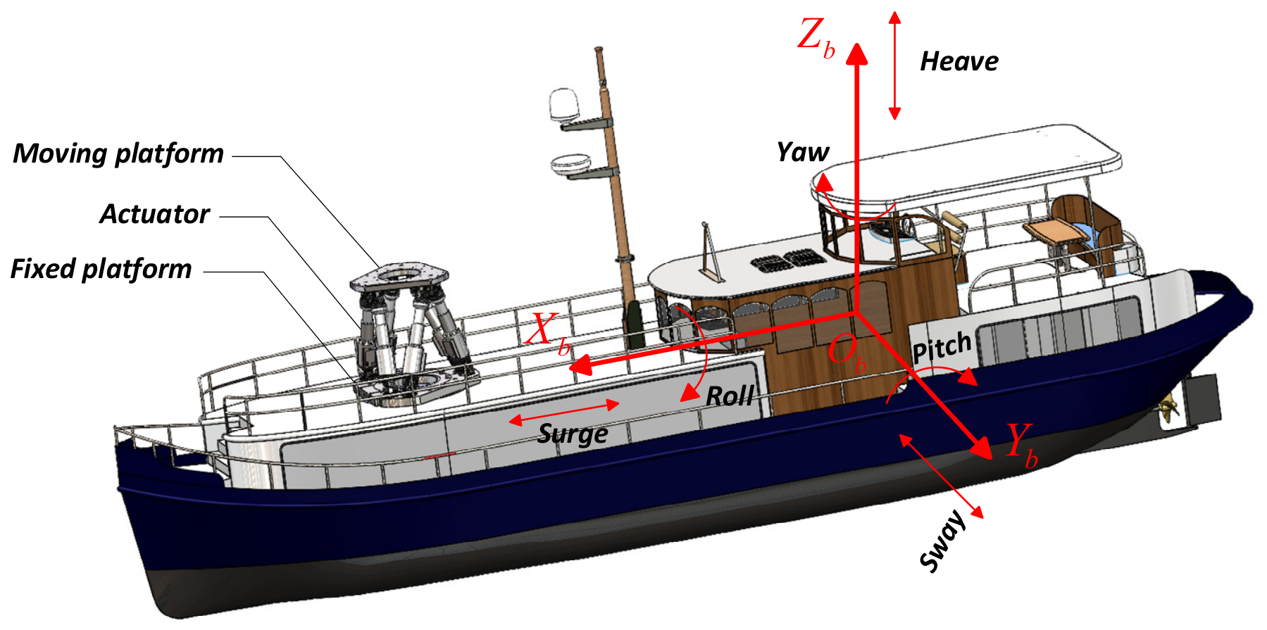
Offshore operations face growing demands for stability and safety due to challenging marine environments, including wind, waves, and currents. Ships experience six-degree-of-freedom (6-DOF) motions, including roll, pitch, yaw, surge, sway, and heave [1], which affect onboard equipment operation, hinder personnel and supply transfer, and limit offshore operation windows. To mitigate these limitations, various wave-compensation technologies have emerged. In particular, the Stewart platform (a 6-DOF wave-compensation parallel robot) has become a widely adopted solution for active wave compensation owing to its high payload capacity, high structural stiffness, and the use of advanced control strategies [2]. However, as a typical multi-input multi-output actuation platform, the Stewart platform requires a high-performance and robust control algorithm, which remains the key to achieving high-precision motion compensation.

To address the control-accuracy problem of Stewart platforms under complex operating conditions, many researchers have carried out extensive studies. In the early stage, classical control methods were most commonly adopted. Şumnu et al. investigated a linear-motor-driven Stewart platform and verified through simulations that PID control can achieve effective pose control. However, the PID controller parameters in that work were mainly determined based on experience, which makes it difficult to maintain consistent performance when model uncertainty and external disturbances vary significantly [3]. Mahapatra et al. studied an electro-hydraulic Stewart platform and still used a control scheme based on linearized single-leg models with independent PI loops. Their experimental results showed that, as the command frequency increased, the oscillation amplitudes of the valve control voltage and leg-length error grew noticeably, indicating a gradual degradation of PI performance [4]. In the field of wave compensation for shipborne Stewart platforms, a number of modern control solutions have been proposed based on detailed dynamic modeling. Cai et al. established a coupled dynamic model using Kane’s method and developed a control structure that combines multi-DOF velocity feedforward compensation with an adaptive robust dual-loop control, achieving high-accuracy joint-space length tracking in the presence of parameter uncertainties and wave disturbances [5]. Based on this framework, a scheme combining a sliding-mode controller with velocity feedforward compensation was also developed to further enhance the suppression of ship-motion disturbances [6]. Furthermore, Wen et al. designed a nonsingular terminal sliding-mode controller from the perspective of the underlying dynamics, and achieved a clear improvement in compensation accuracy and robustness without relying on an exact dynamic model [7]. Chen et al. proposed a 6-DOF wave-compensation system based on Active Disturbance Rejection Control (ADRC) and achieved multiple-fold improvements in both compensation error and compensation smoothness under sea state 4 conditions compared with conventional PI control [8].

Fractional-Order PID control (FOPID), as an extension of conventional integer-order PID control, has in recent years been gradually introduced into wave-compensation-related servo systems and robotic as well as parallel manipulators. Copot et al. applied an FOPID controller to a Stewart platform visual servo system, and experimental comparisons confirmed that FOPID can provide better robustness and tracking performance than PID [9]. Bingul et al. considered joint-space trajectory tracking of a 6-DOF Stewart platform and proposed a fractional-order fuzzy PID (FOFPID) strategy. The controller parameters were optimized offline with a particle swarm optimization algorithm, and simulation and experimental results demonstrated that FOFPID achieves higher tracking accuracy than PID, FOPID, and fuzzy PID under a variety of complex trajectories [10]. Karahan and Karci developed a robust fractional-order fuzzy PID sliding-mode controller for a 6-DOF robotic manipulator, in which the controller parameters were tuned using a hybrid GWO-PSO algorithm [11]. Varga et al. proposed a fractional-order-inspired iterative adaptive control method for robotic systems, further showing the potential of fractional-order control in robot trajectory tracking [12]. Meanwhile, in the area of marine single-degree-of-freedom (single-DOF) compensation, Chen et al. developed a single-DOF active compensation system driven by a permanent magnet synchronous motor (PMSM) and introduced an FOPID controller. The controller parameters were optimized using a hybrid algorithm combining a genetic algorithm and particle swarm optimization. Simulation results showed that, compared with conventional PID control, the improvement was limited to single-DOF heave compensation [13]. Overall, existing studies have demonstrated the effectiveness of fractional-order control and optimization-based tuning in robotic systems, Stewart platforms, and single-DOF wave-compensation systems.

Driven by the ongoing integration of control methods with intelligent algorithms, increasing attention has been paid to wave-compensation systems and related multi-DOF robotic systems. Liu et al. developed a trajectory-tracking control scheme combining a radial basis function neural network with an unknown nonlinear disturbance observer for a 6-DOF parallel robot. Experimental results demonstrated improved tracking accuracy and disturbance rejection under external disturbances [14]. From the perspective of coordinating multiple tasks and constraints, Xing et al. proposed an acceleration-level hierarchical quadratic programming framework with priority-based execution for a mobile manipulator, integrating motion tracking, adaptive motion allocation, and obstacle avoidance within a unified optimization framework [15]. Liu et al. proposed an adaptive control method for an active heave compensation system by combining a neural network with the beetle antennae search algorithm. Relative to traditional approaches, the maximum compensation error is reduced by about 70%, and the mean squared error during heave motion is reduced by about 40% [16]. Tang et al. designed a fuzzy PID controller for a pendulum-type wave-compensation platform, which shortens the system response time and reduces attitude oscillation amplitudes compared with a PID controller [17]. Chen et al. proposed an inner-outer dual-loop online Adaptive Model Predictive Control (AMPC) strategy. Experiments under sea state 4 conditions showed superior compensation accuracy and stability compared to conventional control methods [18].

The above literature reveals that wave-compensation systems employ three main categories of control strategies: (1) classical approaches, such as PI/PID and combined feedforward-feedback control [19]; (2) modern methods, including robust, sliding-mode, and adaptive control; and (3) intelligent strategies, such as fuzzy control, neural-network-based control, and model predictive control [20]. In addition, the application of FOPID control to wave-compensation-related servo systems has also started to appear in recent years. In classical control schemes, a shipborne Stewart platform is characterized by strong nonlinearity and complex disturbances. Although PI control is relatively easy to implement and relies less on an accurate mathematical model, it is difficult to adapt to time-varying dynamics, and thus it is hard to achieve satisfactory dynamic tracking performance [21]. In modern control schemes, an accurate plant model is often required. Otherwise, control accuracy can significantly decrease. Meanwhile, the control structures are usually complex and involve many parameters, which increases the difficulty of engineering implementation and tuning [22]. For intelligent control, as well as control methods that combine fractional-order control with intelligent algorithms, there are generally issues such as complex control structures, high-dimensional parameter settings, and relatively large computational demands, both online and offline. Moreover, neural-network-based methods require a large amount of training data, and their compensation performance is prone to degradation under abrupt load changes and extreme environments, which constrains the system’s real-time performance and engineering feasibility [23]. Despite these advances, optimized fractional-order triple-loop control for PMSM-driven 6-DOF shipborne Stewart platforms remains insufficiently investigated, particularly regarding mechanism-actuator coupling, explicit six-leg tracking-objective formulation, and comprehensive evaluation under diverse excitation and disturbance conditions.

To address these research gaps, it is necessary to develop a control scheme that offers a better trade-off among structural simplicity, robustness, and tracking accuracy. By introducing fractional integral operators into a PI controller, Fractional-Order PI (FOPI) control extends the conventional PI structure. On the one hand, it retains the practical merits of PI control, such as an intuitive structure, ease of implementation, and weak dependence on an accurate model. On the other hand, the fractional-order integral action enhances the ability to represent and regulate complex system dynamics and low-frequency disturbances, thereby providing better overall performance than integer-order PI control under nonlinear and time-varying conditions [24]. Compared with FOPID, FOPI avoids the additional fractional-order derivative term, which reduces the number of parameters to be tuned and avoids possible amplification of high-frequency measurement noise [25]. This is consistent with the characteristics of shipborne wave-compensation systems, where the dominant disturbances are mainly concentrated in the low-frequency range. Furthermore, the FOPI controller has a clear parametric form with a moderate number of parameters, which makes it convenient to combine with metaheuristic optimization algorithms for global parameter search. In this way, the limitations of traditional tuning, which is experience-dependent and prone to local optima, can be systematically alleviated [26]. Among commonly used metaheuristic optimization algorithms, particle swarm optimization (PSO) has a simple structure but may suffer from premature convergence when the population rapidly gathers around the current best solution. Genetic algorithm (GA) has good global search ability, but its selection, crossover, and mutation operations increase the tuning complexity for continuous controller parameters. Whale Optimization Algorithm (WOA) provides competitive exploitation ability, whereas its later-stage search behavior may still be strongly affected by the current best individual. In contrast, tuna swarm optimization (TSO) algorithm integrates spiral foraging and parabolic foraging strategies, allowing the population to explore the search space broadly while refining candidate solutions in promising regions. Therefore, TSO is selected to optimize the FOPI parameters in this paper. Accordingly, a TSO-based FOPI (TSO-FOPI) triple-loop wave-compensation control scheme is developed for a PMSM-driven shipborne Stewart platform, aiming to achieve high-accuracy and robust compensation of 6-DOF wave disturbances while maintaining implementation simplicity. The main contributions of this paper are as follows:

(1) This work is the first to apply a TSO-based triple-loop FOPI control scheme to shipborne 6-DOF wave compensation. By exploiting the global search and dynamic optimization capability of TSO, the proposed approach alleviates the common drawbacks of conventional parameter tuning, such as strong reliance on experience and a tendency to fall into local optima.

(2) A triple-loop FOPI control strategy is proposed for the shipborne Stewart platform. The proposed strategy addresses the inherent difficulty of conventional PI control in balancing compensation accuracy, response smoothness, and wideband disturbance-rejection performance.

The remainder of this article is organized as follows. Section 2 introduces the dynamic modeling of the Stewart platform and the modeling analysis of the actuators. Section 3 describes the controller design and provides the corresponding stability analysis. Section 4 provides the simulation results and discussion. Section 5 concludes the article.

2. Wave Compensation System Based on Stewart Platform

In a shipborne Stewart wave-compensation system, the desired 6-DOF pose of the moving platform cannot be directly imposed on the actuators. Instead, it must be mapped into the desired leg lengths of the six actuated limbs through the inverse kinematics of the Stewart platform. In addition, the dynamic interactions among the moving platform, the actuator legs, and the PMSM-driven transmission system directly affect the required driving force and the achievable compensation accuracy. Therefore, accurate mathematical modeling of both the Stewart platform and the PMSM is essential for the subsequent design of the triple-loop TSO-FOPI control strategy.

2.1. Mathematical Model of a Stewart Platform

As shown in Figure 1, in a complex marine environment, winds and waves can induce 6-DOF motions of a ship, including three translational motions (sway, surge, and heave) and three rotational motions (roll, pitch, and yaw). As the core component of an attitude-compensation system, the Stewart platform is a classical parallel mechanism consisting of a fixed platform, a moving platform, and six high-precision actuated legs. For each leg, the actuation unit integrates a PMSM, a precision reduction mechanism, and a ball-screw transmission system. The leg is connected to the fixed platform through a universal joint at the bottom and to the moving platform through a spherical joint at the top, forming a compliant connection that accommodates multi-directional motion. By measuring the ship motion states in real time and dynamically computing the required leg extensions using an inverse kinematics model, the platform actuates the moving platform to maintain a stable attitude in the inertial frame [27]. As a result, the system can effectively reduce the adverse effects of ship oscillations on deck-to-deck material transfer and personnel movement, thereby improving operational safety and reliability [28].

For convenience of analysis, the following coordinate frames are defined (as shown in Figure 2): (1) O_b-x_by_bz_b denotes the world or inertial frame, where the x_b-axis is parallel to the surge direction, the y_b-axis is parallel to the sway direction, and the z_b-axis is parallel to the heave direction; (2) O_m-x_my_mz_m denotes the reference frame of the fixed platform, whose origin O_m is located at the geometric center of the fixed platform, which is typically also the installation center of the inertial sensor. Moreover, the x_m-axis is parallel to the x_b-axis and the z_m-axis is parallel to the z_b-axis; (3) O_s-x_sy_sz_s denotes the reference frame of the moving platform, whose origin O_s is located at the geometric center of the moving platform, and each axis is parallel to the corresponding axis of frame O_m. The corresponding rotation matrix can be expressed as [29]:

$$\mathit{R}=\left(\begin{array}{ccc}\cos \alpha \cos \beta & \cos \alpha \sin \beta \sin \gamma -\sin \alpha \cos \gamma & \sin \alpha \sin \gamma +\cos \alpha \sin \beta \cos \gamma \\ \sin \alpha \cos \beta & \cos \alpha \cos \gamma +\sin \alpha \sin \beta \sin \gamma & \sin \alpha \sin \beta \cos \gamma -\cos \alpha \sin \gamma \\ -\sin \beta & \cos \beta \sin \gamma & \cos \beta \cos \gamma \end{array}\right)$$

(1)

where $\gamma ,\beta ,\mathrm{and} \alpha$ denote the roll, pitch, and yaw angles, respectively.

For the translational motion of the moving platform relative to the fixed platform in the Stewart platform, the displacement is expressed as a vector: ${\mathit{p}=\left[x,y,z\right]}^{\mathrm{T}}$. Therefore, the pose of the Stewart platform can be described by the following generalized coordinate vector:

$$\mathit{q}={\left[x,y,z,\gamma ,\beta ,\alpha \right]}^{\mathrm{T}}$$

(2)

The length of each actuator leg can be expressed as:

$$l_i=‖\mathit{p}+\mathit{R}{\mathit{p}}_{\mathit{i}}-{\mathit{b}}_{\mathit{i}}‖, i=1,\dots ,6$$

(3)

where $i$ denotes the index of the leg, ${\mathit{p}}_{\mathit{i}}$ represents the coordinates of the upper joint point in the moving frame, and ${\mathit{b}}_{\mathit{i}}$ represents the coordinates of the lower joint point in the fixed frame.

For the moving platform, the dynamic equation can be obtained from the Newton–Euler equation as [30]:

$${\left({\displaystyle \genfrac{}{}{0pt}{}{\mathit{n}}{\mathit{R}{\mathit{r}}_{\mathit{i}}\times \mathit{n}}}\right)}_{6\times 6}{\mathit{f}}_{\mathit{a}}=\left(\begin{array}{cc}{m}_p{\mathit{I}}_3& \mathbf{0}\\ \mathbf{0}& {\mathit{I}}_{\mathit{p}}\end{array}\right)\left({\displaystyle \genfrac{}{}{0pt}{}{\ddot{\mathit{p}}}{\dot{\mathit{\omega }}}}\right)+\left(\begin{array}{cc}\mathbf{0}& \mathbf{0}\\ \mathbf{0}& \mathsf{\Omega }{\mathit{I}}_{\mathit{p}}\end{array}\right)\left({\displaystyle \genfrac{}{}{0pt}{}{\dot{\mathit{p}}}{\mathit{\omega }}}\right)+\left({\displaystyle \genfrac{}{}{0pt}{}{m_p\mathit{g}}{\mathbf{0}}}\right)$$

(4)

where $\mathit{n}$ is the axial unit vector of the leg, ${\mathit{r}}_{\mathit{i}}$ is the position vector from the center of mass of the moving platform to its hinge point, ${\mathit{f}}_{\mathit{a}}$ is the output force of the electric cylinder in the leg, $m_p$ is the mass of the moving platform, and ${\mathit{I}}_3$ is the third-order unit matrix. ${\mathit{I}}_{\mathit{p}}$ is the moment of inertia of the moving platform, $\mathsf{\Omega }$ denotes the skew symmetric matrix of an angular velocity vector, and $\mathit{\omega }$ is the angular velocity of the moving platform’s center of mass with respect to the inertial frame. $\mathit{g}$ is the vector of gravitational acceleration. The above equation can be written in a general form as:

$${\mathit{J}}_{\mathit{s}}^T{\mathit{f}}_{\mathit{a}}={\mathit{M}}_{\mathit{p}}\ddot{\mathit{x}}+{\mathit{C}}_{\mathit{p}}\dot{\mathit{x}}+{\mathit{G}}_{\mathit{p}}$$

(5)

$${\mathit{J}}_{\mathit{s}}={\left(\begin{array}{cc}{\mathit{n}}_1^{\mathrm{T}}& {\left[\mathit{R}{\mathit{r}}_1\times {\mathit{n}}_1\right]}^{\mathrm{T}}\\ {\mathit{n}}_2^{\mathrm{T}}& {\left[\mathit{R}{\mathit{r}}_2\times {\mathit{n}}_2\right]}^{\mathrm{T}}\\ ⋮& ⋮\\ {\mathit{n}}_6^{\mathrm{T}}& {\left[\mathit{R}{\mathit{r}}_6\times {\mathit{n}}_6\right]}^{\mathrm{T}}\end{array}\right)}_{6\times 6}$$

(6)

where ${\mathit{J}}_{\mathit{s}}$ is the Jacobian matrix relating the extension velocities of the six legs to the generalized velocity of the moving platform, ${\mathit{M}}_{\mathit{p}}$, ${\mathit{C}}_{\mathit{p}}$, and ${\mathit{G}}_{\mathit{p}}$ are the generalized mass matrix, Coriolis matrix, and gravity vector of the moving platform, $\dot{\mathit{x}}$ is the generalized velocity vector of the moving platform’s center of mass in the inertial frame, and $\ddot{\mathit{x}}$ is the generalized acceleration vector. To calculate the influence of each leg on the moving platform, the leg forces need to be projected to the center of mass of the moving platform. The Jacobian matrix relating the velocity of the piston-rod center of mass to that of the upper joint point is given by:

$${\mathit{J}}_{\mathit{d}\mathit{i}}={\mathit{I}}_{\mathbf{3}}-{\displaystyle \frac{l_a}{\left|l_i\right|}}{\mathit{P}}_{\mathit{i}}$$

(7)

where $l_a$ denotes the distance from the piston-rod center of mass to the upper joint point, $l_i$ denotes the extension length of the leg, and ${\mathit{P}}_{\mathit{i}}={\mathit{I}}_{\mathbf{3}}-{\mathit{n}}_{\mathit{i}}{{\mathit{n}}_{\mathit{i}}}^{\mathrm{T}}$, ${\mathit{n}}_{\mathit{i}}$ is the unit vector of the leg.

Let the mass of the piston rod be $m_c$, then the piston-rod gravity projected to the moving platform’s center of mass can be expressed as:

$${\mathit{f}}_{\mathit{c}\mathit{i}}=-{\mathit{J}}_{{\mathit{B}}_{\mathit{i}}}^{\mathrm{T}}{\mathit{J}}_{\mathit{d}\mathit{i}}^{\mathrm{T}}{m}_c\mathit{g}$$

(8)

where ${\mathit{B}}_{\mathit{i}}$ denotes the position vector of the upper joint point in the inertial frame. ${\mathit{J}}_{{\mathit{B}}_{\mathit{i}}}$ is the Jacobian that maps the platform generalized velocity to the velocity of the $i$-th upper joint point.

Considering the inertial force of the leg, its projection to the moving platform’s center of mass can be expressed as:

$${\mathit{f}}_{\mathit{g}}={\mathit{M}}_{\mathit{g}}\ddot{\mathit{x}}+{\mathit{C}}_{\mathit{g}}\dot{\mathit{x}}$$

(9)

where ${\mathit{M}}_{\mathit{g}}$ is the mass matrix of the leg, and ${\mathit{C}}_{\mathit{g}}$ is the corresponding centrifugal and Coriolis matrices of the leg.

Therefore, the multibody dynamic equation of the Stewart platform can be written as:

$${\mathit{J}}_{\mathit{s}}^{\mathrm{T}}{\mathit{f}}_{\mathit{a}}={\mathit{M}}_{\mathit{z}}{{\mathit{J}}_{\mathit{s}}}^{-1}\ddot{\mathit{L}}+\left({\mathit{C}}_{\mathit{z}}-{\mathit{M}}_{\mathit{z}}{{\mathit{J}}_{\mathit{s}}}^{-1}\dot{{\mathit{J}}_{\mathit{s}}}\right){{\mathit{J}}_{\mathit{s}}}^{-1}\dot{\mathit{L}}+{\mathit{G}}_{\mathit{z}}$$

(10)

where ${\mathit{M}}_{\mathit{z}}={\mathit{M}}_{\mathit{p}}+{\mathit{M}}_{\mathit{g}},{\mathit{C}}_{\mathit{z}}={\mathit{C}}_{\mathit{p}}+{\mathit{C}}_{\mathit{g}},{\mathit{G}}_{\mathit{z}}={\mathit{G}}_{\mathit{p}}+{\displaystyle {\sum }_{i=1}^6}{\mathit{f}}_{\mathit{c}\mathit{i}},\dot{\mathit{L}}={\mathit{J}}_{\mathit{s}}\dot{\mathit{x}},\ddot{\mathit{L}}=\dot{{\mathit{J}}_{\mathit{s}}}\dot{\mathit{x}}+{\mathit{J}}_{\mathit{s}}\ddot{\mathit{x}}$. $\dot{\mathit{L}}$ denotes the leg extension velocity, and $\ddot{\mathit{L}}$ denotes the leg acceleration.

The above dynamic model accurately characterizes the inverse dynamics of the Stewart platform in joint space. Through the mapping of the Jacobian matrix, the axial driving forces of the legs are linked to the platform displacement, velocity, and acceleration. It further clarifies the coupled force-motion mechanism inherent in parallel mechanisms: the spatial motion of the platform is driven cooperatively by the six legs, while the leg forces are mutually coupled through the geometric constraints of the structure. This coupling is mainly reflected in the Jacobian matrix, which varies online with the platform pose, as well as in the nonlinear Coriolis matrix, thereby providing a theoretical basis for implementing control strategies in practical systems.

2.2. Mathematical Model of PMSM

In this study, a permanent magnet synchronous motor with surface permanent magnets is selected as the core actuator of the Stewart platform, leveraging its advantages of a simple structure, low cost, and small rotor inertia, while a ball-screw mechanism is used to realize the extension and retraction of each leg. For simplicity, three ideal assumptions are adopted: magnetic saturation is neglected, eddy-current and hysteresis losses are ignored, and the three-phase currents are assumed to be sinusoidal [31].

The three-phase voltage equations of the PMSM in the stationary three-phase reference frame can be written as:

$${\mathit{u}}_{3s}={\mathit{r}}_{3s}{\mathit{i}}_{3s}+{\displaystyle \frac{\mathrm{d}}{\mathrm{d}t}}{\mathit{\psi }}_{3s}$$

(11)

where ${\mathit{\psi }}_{3s}$ is the flux linkages of the three-phase windings, and ${\mathit{u}}_{3s}$, ${\mathit{i}}_{3s}$, ${\mathit{r}}_{3s}$ denote the phase voltage, current, and resistance of the three-phase winding.

For convenience in controller design, the PMSM model is usually expressed in the synchronous rotating d-q reference frame [32]. Accordingly, the stator voltage equations can be written as:

$$\left\{\begin{array}{c}{u}_d=R_s{i}_d+L_d{\displaystyle \frac{\mathrm{d}}{\mathrm{d}t}}{i}_d-{\omega }_e{L}_q{i}_q\\ u_q=R_s{i}_q+L_q{\displaystyle \frac{\mathrm{d}}{\mathrm{d}t}}{i}_q+{\omega }_e{L}_d{i}_d+{\omega }_e{\psi }_m\end{array}\right.$$

(12)

where $u_d$ and $u_q$ denote the d-q axis components of the stator voltage; $i_d$ and $i_q$ denote the d-q axis components of the stator current; $L_d$ and $L_q$ denote the d-q axis components of the inductances; $R_s$ is the stator resistance; ${\omega }_e$ is the electrical angular speed; ${\psi }_m$ denotes the permanent-magnet flux linkage [33].

Accordingly, the electromagnetic torque equation can be written as:

$$T_e={\displaystyle \frac{3P_n{i}_q}{2}}\left[i_d\left(L_d-L_q\right)+{\psi }_m\right]$$

(13)

For the surface-mounted PMSM adopted in this study, $L_d=L_q$. Therefore, the electromagnetic torque equation used in the simulation is simplified as:

$$T_e={\displaystyle \frac{3P_n{i}_q}{2}}{\psi }_m$$

(14)

where $P_n$ is the number of pole pairs of the PMSM. The mechanical motion equation of the motor can be written as:

$$J_m{\displaystyle \frac{\mathrm{d}{\omega }_m}{\mathrm{d}t}}=T_e-T_L-B_m{\omega }_m$$

(15)

where ${\omega }_m$ is the mechanical angular speed of the motor, $J_m$ is the rotational inertia, $T_L$ is the load torque, and $B_m$ is the damping coefficient.

3. Control Task

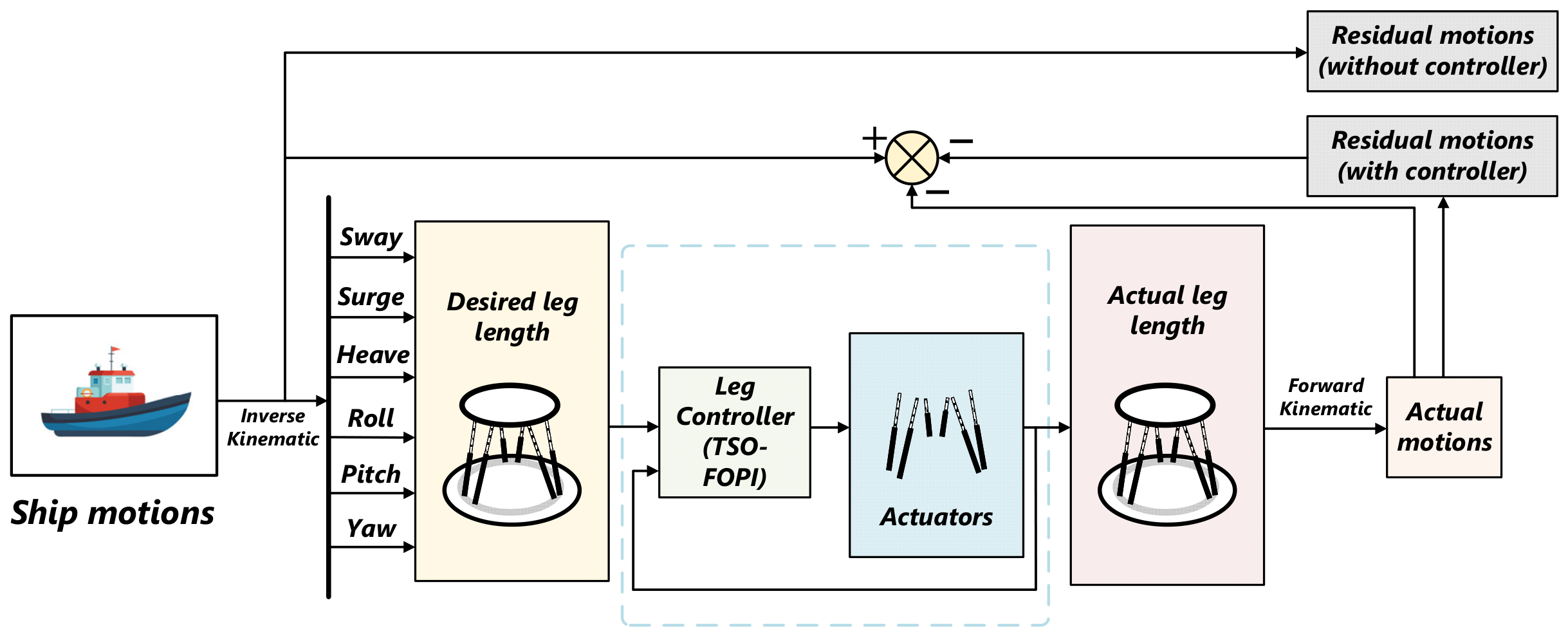
The conventional control strategies for a Stewart platform generally follow two paradigms: task-space control and joint-space control. In task-space control, the pose of the moving platform is taken as the direct control objective, which typically requires forward kinematics to estimate the 6-DOF motion. However, the task-space dynamic model is highly nonlinear and strongly coupled, accurate modeling is difficult, and the real-time computational demand is high. As a result, this approach is rarely adopted for Stewart platforms. In joint-space control, the desired platform pose is converted into the target lengths of the actuator legs via inverse kinematics, and the actuators are then driven directly. This method offers higher computational efficiency and avoids the uncertainties introduced by forward kinematics, making it more suitable for real-time control [34]. Therefore, based on an inverse-dynamics analysis, this article transforms the dynamic attitude of a Stewart platform into the target lengths of each leg. Meanwhile, a TSO-FOPI triple-loop control algorithm is adopted to precisely regulate the positions of the PMSMs driving the legs, thereby ensuring high-precision motion control of the platform.

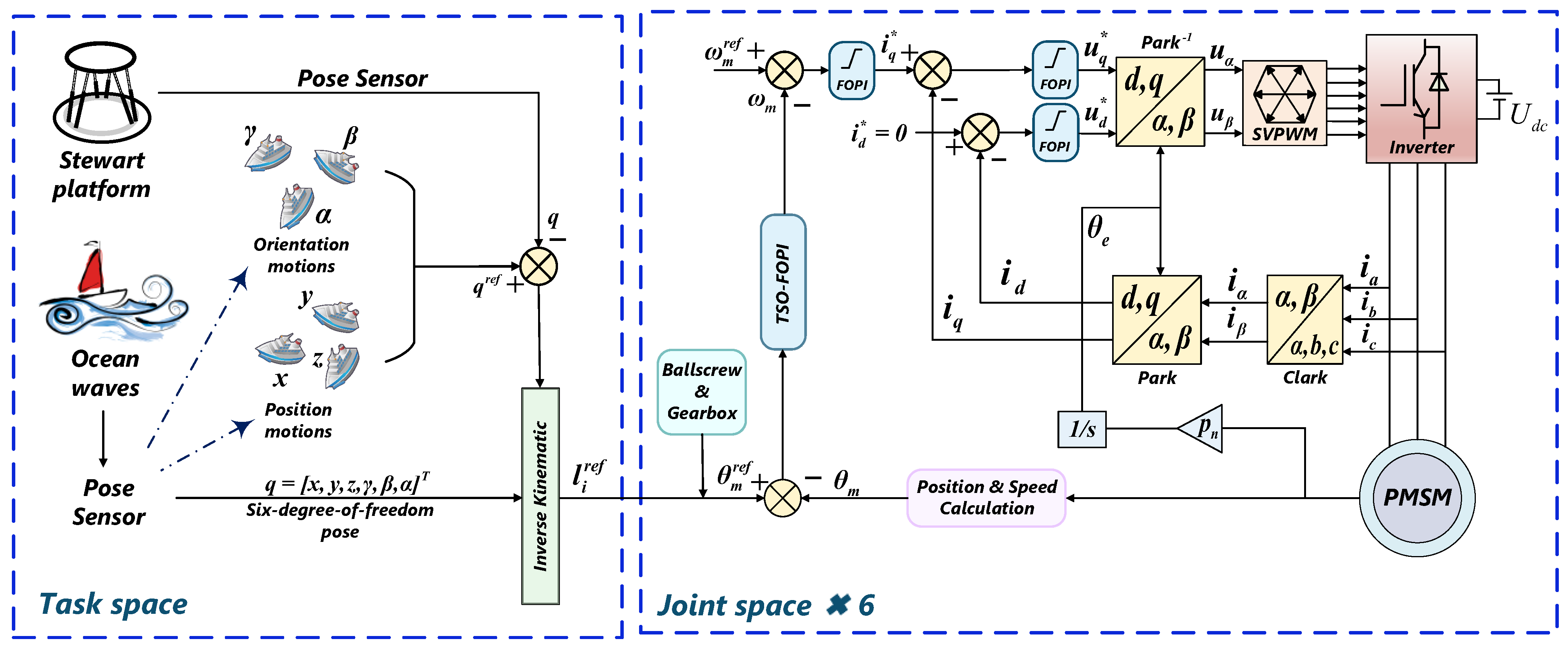
The PMSM control strategy adopted for the Stewart platform in this article is based on a triple-loop control architecture, as shown in Figure 3. In this scheme, the current loop, speed loop, and position loop all employ an FOPI control law, and a TSO-FOPI design is further introduced in the position loop. The current loop regulates the stator current and suppresses high-frequency current fluctuations. The speed loop regulates the motor speed and provides the reference signal for the inner current loop. The position loop focuses on accurate position regulation to improve the overall control accuracy. Based on this architecture, the 6-DOF pose-compensation task is converted into the joint-space position tracking of six PMSM-driven actuator legs. Therefore, the proposed TSO-FOPI scheme provides a practical control framework for multi-DOF wave compensation of Stewart platform systems [8,27,28,34].

3.1. TSO-FOPI Control Scheme

This paper adopts a triple-loop control strategy consisting of a position loop, a speed loop, and a current loop. Both the current loop and the speed loop employ FOPI controllers, whereas the position loop adopts a TSO-FOPI controller. The TSO-FOPI controller is essentially an FOPI controller whose parameters are optimized by TSO. Owing to the global optimization capability of TSO, the proposed method alleviates the dependence on experience in conventional FOPI tuning and improves the system’s adaptability to nonlinearity, time-varying behavior, and model uncertainty.

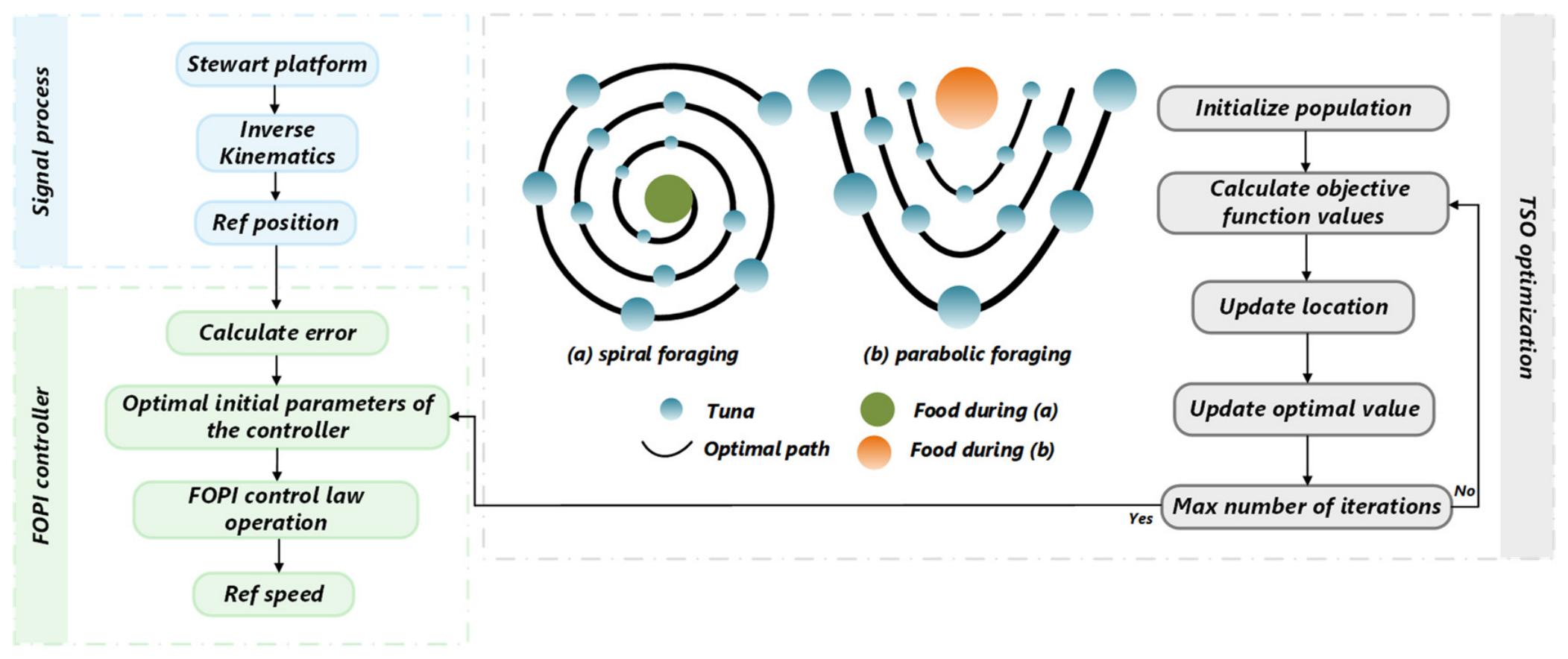
The offline TSO-based parameter optimization process for the proposed position-loop FOPI controller is shown in Figure 4. First, the initial tuna population is generated within the prescribed ranges of the FOPI controller parameters. Then, the objective function value of each candidate solution is calculated, and the current best individual is updated accordingly. During the iterative search process, the positions of the tuna individuals are updated through the spiral and parabolic foraging strategies. When the maximum number of iterations is reached, the best individual obtained from the search is selected as the optimized parameter set for the position-loop FOPI controller.

Compared with conventional PI control, the proposed TSO-FOPI control strategy introduces the fractional integral order $\lambda$, providing an additional degree of freedom for shaping the closed-loop response. Compared with manually tuned FOPI control, the position-loop parameters $K_p$, $K_i$, and $\lambda$ are determined through an explicitly formulated offline optimization problem rather than experience-based trial and error. Compared with FOPID control, the proposed method avoids the additional fractional derivative term and the associated tuning complexity and potential amplification of high-frequency measurement noise. In addition, unlike online adaptive or learning-based methods, the TSO is completed before closed-loop operation and therefore introduces no online parameter-update burden.

3.2. FOPI Controller Structure

FOPI control integrates fractional-order calculus with conventional PI control. Fractional calculus is a generalization of integer-order calculus, and its theoretical framework and numerical implementation constitute the foundation of fractional-order control. Therefore, an FOPI controller can be regarded as an extension of a standard PI controller. Compared with a conventional PI controller, an FOPI controller introduces an additional tuning parameter: a non-integer fractional integral order $\lambda$. This significantly increases design flexibility and, consequently, enhances the controller’s control capability [35].

The differential equation of the ${PI}^{\lambda }$ controller is given as follows:

$$u\left(t\right)=K_{p}e\left(t\right)+K_i{D}^{-\lambda }e\left(t\right)$$

(16)

where $0<\lambda \le 1$; $u\left(t\right)$ is the controller output; $e\left(t\right)=r\left(t\right)-y\left(t\right)$, $e\left(t\right)$ is the system error signal; $r\left(t\right)$ denotes the reference input; $y\left(t\right)$ denotes the actual system output; $K_p$ is the proportional gain; $K_i$ is the integral gain. $D^{-\lambda }$ is the $\lambda$-order fractional integral operator.

The flexibility in selecting $\lambda$ enables the controller to model the dynamic behavior of physical systems more accurately. Fractional-order calculus allows more general response forms that include memory effects, so the controller can take into account both past and present system states. This capability inherently improves control performance and accuracy.

The transfer function of a typical FOPI controller can be obtained as follows:

$$C_{FOPI}\left(s\right)=K_p+K_i{s}^{-\lambda }$$

(17)

where $s^{-\lambda }$ denotes the Laplace transform of the fractional-order integral operator.

In this paper, Oustaloup’s recursive approximation is employed to approximate the fractional-order integral operator $s^{-\lambda }$ over the prescribed frequency range $\left[{\omega }_b, {\omega }_h\right]$. The fractional-order operator is represented by a finite-dimensional rational transfer function consisting of 2N + 1 first-order pole–zero pairs [36,37]:

$$s^{-\lambda }\approx {\omega }_h^{-\lambda }{\displaystyle \prod _{k=-N}^N}{\displaystyle \frac{s+{\omega }_k^{\prime }}{s+{\omega }_k}}$$

(18)

where ${\omega }_k^{\prime }={\omega }_b{\left({\displaystyle \frac{{\omega }_h}{{\omega }_b}}\right)}^{{\displaystyle \frac{k+N+\left(1+\lambda \right)/2}{2N+1}}}$, ${\omega }_k={\omega }_b{\left({\displaystyle \frac{{\omega }_h}{{\omega }_b}}\right)}^{{\displaystyle \frac{k+N+\left(1-\lambda \right)/2}{2N+1}}}$, ${\omega }_b$ and ${\omega }_h$ denote the lower and upper bounds of the approximation frequency range, respectively. $N$ is the approximation-order parameter, while ${\omega }_k^{\prime }$ and ${\omega }_k$ represent the recursively distributed zero and pole frequencies, respectively. Increasing $N$ generally improves the approximation accuracy within the prescribed frequency range, at the cost of increased computational complexity.

The approximation-order parameter is selected as $N=5$, and the approximation frequency range is set to $\left[{\omega }_b, {\omega }_h\right]=\left[{10}^{-3},{10}^3\right]$. According to the formulation in Equation (18), $N=5$ results in 11 recursively distributed first-order pole–zero pairs. This setting provides a compromise between approximation accuracy and computational complexity and covers the principal frequency range considered in the platform wave-compensation and cascaded-loop simulations.

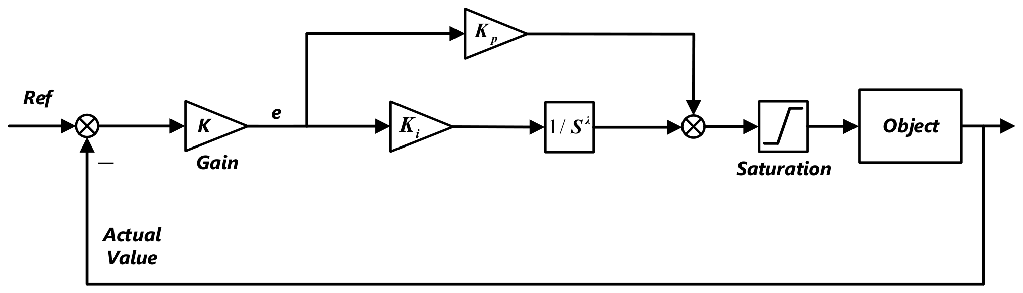
If the three parameters $K_p$, $K_i$, and $\lambda$ of the FOPI controller are properly selected, better control performance than that of an integer-order PI controller can be achieved. The FOPI control for the current loop and the speed loop is shown in Figure 5.

3.3. Tuna Swarm Optimization Algorithm

During the parameter tuning of an FOPI controller, the initial values of $K_{p0} ,K_{i0}$, and $\lambda$ are directly related to controller stability, dynamic response, and overall system control performance. Conventional manual tuning relies heavily on human experience; each trial is time-consuming and still unable to explore the full parameter space. As a result, the obtained settings are often prone to being trapped in local optima. Employing metaheuristic optimization methods for global parameter tuning of controllers can eliminate empirical tuning and achieve superior control performance [38]. Therefore, this paper employs TSO to optimize the initial parameters of the FOPI controller. Compared with other metaheuristic optimization methods, a key feature of TSO is that it is inspired by two cooperative foraging behaviors of tuna swarms: spiral foraging and parabolic foraging [39].

The population update process of TSO for optimization in the search space can be expressed as follows:

$${\mathit{X}}_i^{int}=\mathit{r}⨀ \left({\mathit{x}}_{\mathrm{ub}}-{\mathit{x}}_{\mathrm{lb}}\right)+{\mathit{x}}_{\mathrm{lb}}, i=1, 2,\cdots ,NP$$

(19)

where ${\mathit{X}}_i^{int}$ denotes the $i$-th initial individual; ${\mathit{x}}_{\mathrm{ub}}$ and ${\mathit{x}}_{\mathrm{lb}}$ are the upper-bound and lower-bound vectors of the search space, respectively. $NP$ is the population size of the tuna swarm, and $\mathit{r}$ is a random vector uniformly distributed in [0, 1]. $⨀$ denotes the element-wise (Hadamard) product.

Spiral foraging refers to the behavior in which tuna form a tight spiral formation to pursue schools of small fish whose swimming direction changes continuously. When a small subgroup in the swarm moves first in a certain direction to chase the prey, the nearby tuna quickly adjust their headings and cooperate to encircle the target. Moreover, because the formation is compact, neighboring tuna can share information efficiently, which helps improve the overall foraging effectiveness. Motivated by this behavior, the spiral foraging strategy can be expressed as follows:

If rand $\ge {\displaystyle \frac{q}{q_{max}}}$, rand denotes a scalar random number uniformly distributed over [0, 1], then:

$$X_i^{q+1}=\left\{\begin{array}{c}{\alpha }_1·\left(X_{best}^q+\beta ·\left|X_{best}^q-X_i^q\right|\right)+{\alpha }_2·{X_i}^q, i=1\\ {\alpha }_1·\left(X_{best}^q+\beta ·\left|X_{best}^q-X_i^q\right|\right)+{\alpha }_2·X_{i-1}^q, i=\mathrm{2,3},\cdots ,NP\end{array}\right.$$

(20)

$${\alpha }_1=m+\left(1-m\right)·{\displaystyle \frac{q}{q_{max}}} , {\alpha }_2=\left(1-m\right)-\left(1-m\right)·{\displaystyle \frac{q}{q_{max}}}$$

(21)

where $\beta =e^{bl}·\cos 2\pi b,l=\exp \left(3\cos \left(\left(\left(q_{max}+{\displaystyle \frac{1}{q+1}}\right)-1\right)\pi \right)\right),$ $b$ is a random variable uniformly distributed in the interval [0, 1]. $q$ denotes the current iteration number, $q_{max}$ denotes the maximum number of iterations, $X_i^{q+1}$ is the $i$-th individual at iteration $q+1$, $X_{best}^q$ is the current best individual, and ${\alpha }_1$ and ${\alpha }_2$ are weighting coefficients that guide the individual to move toward the best individual and the previous individual, respectively. $m$ is a constant that controls the extent to which tuna individuals follow the current best individual and the previous individual during the early search stage. The parameter m is a preset constant rather than an adaptively selected variable. m is set to 0.7 and remains unchanged throughout the optimization process [39]. Accordingly, as the iteration number $q$ increases from 0 to $q_{max}$, ${\alpha }_1$ increases linearly from 0.7 to 1, whereas ${\alpha }_2$ decreases linearly from 0.3 to 0. This variation gradually strengthens the guidance of the current best individual while reducing the influence of the previous individual.

When a food source is located around the tuna swarm, tuna can forage effectively within the search space. However, when the current best individual fails to locate the food source, it cannot guide the swarm efficiently. Therefore, a randomly generated reference point is introduced in the search space to facilitate spiral searching, thereby preserving the global search capability of TSO. The corresponding mathematical model is given as follows:

If rand $<{\displaystyle \frac{q}{q_{max}}}$, then:

$$X_i^{q+1}=\left\{\begin{array}{c}{\alpha }_1·\left(X_{\mathrm{rand}}^q+\beta ·\left|X_{\mathrm{rand}}^q-X_i^q\right|\right)+{\alpha }_2·X_i^q, i=1\\ {\alpha }_1·\left(X_{\mathrm{rand}}^q+\beta ·\left|X_{\mathrm{rand}}^q-X_i^q\right|\right)+{\alpha }_2·X_{i-1}^q, i=\mathrm{2,3},\cdots ,NP\end{array}\right.$$

(22)

where $X_{\mathrm{rand}}^q$ denotes a reference point randomly generated in the search space.

In addition, tuna can form a parabolic formation around the food source, leading to a parabolic cooperative foraging behavior. During the foraging process, these two strategies are selected with equal probability, each with a selection probability of 0.5. The mathematical model can be described as follows:

$$X_i^{q+1}=\left\{\begin{array}{c}{X}_{best}^q+\mathrm{r}\mathrm{a}\mathrm{n}\mathrm{d}·\left(X_{best}^q-X_i^q\right)+HF·p^2·\left(X_{best}^q-X_i^q\right), if \mathrm{r}\mathrm{a}\mathrm{n}\mathrm{d}<0.5\\ HF·p^2·X_i^q , if \mathrm{r}\mathrm{a}\mathrm{n}\mathrm{d}\ge 0.5\end{array}\right.$$

(23)

$$p={\left(1-{\displaystyle \frac{q}{q_{max}}}\right)}^{{\displaystyle \frac{q}{q_{max}}}}$$

(24)

where $HF$ takes the value of 1 or −1. $p$ is not an independently selected parameter. It is an iteration-dependent adjustment coefficient automatically calculated according to Equation (24). As the iteration proceeds, $p$ decreases nonlinearly from a value close to 1 to 0. Through the $p^2$ term in Equation (23), the magnitude of the population update is gradually reduced, thereby supporting broad exploration in the early stage and refined exploitation in the later stage.

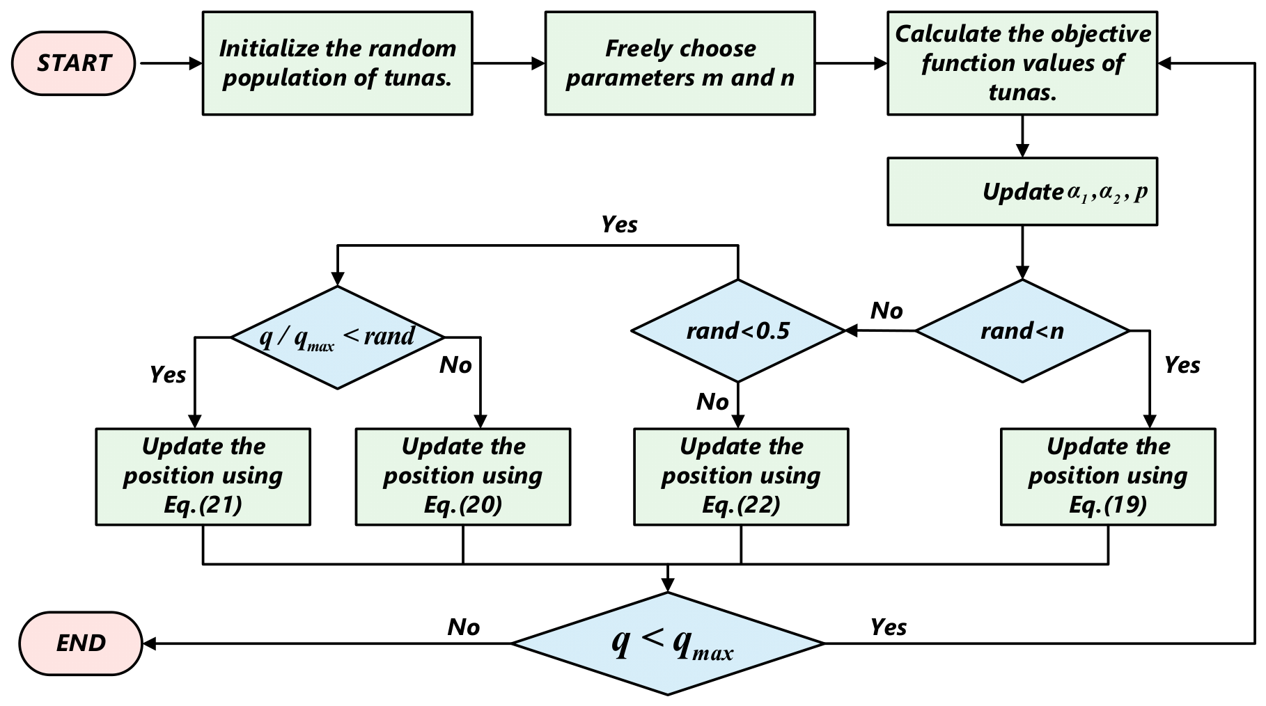
For the TSO process, a population is first randomly initialized within the search space. At each iteration, each individual updates its position in the search space with probability n. Throughout the optimization, all individuals in TSO are continuously updated until the stopping criteria are satisfied, after which the best individual and its corresponding objective function value are returned. The flowchart in Figure 6 illustrates the detailed steps of TSO.

In this paper, the TSO-FOPI controller employs TSO to perform global optimization of the FOPI controller parameters, resulting in an optimization dimension of three. The population size of the tuna swarm directly affects the global search capability of the algorithm as well as the coverage of the search space. A population that is too small may cause the algorithm to be trapped in local optima, whereas an excessively large population significantly increases the computational cost of each simulation. Considering the nonlinear complexity of the Stewart platform system and the associated simulation burden, the population size is set to 180 in this study. The maximum number of iterations determines both the convergence depth and the overall computational time. To avoid insufficient exploration caused by premature convergence while maintaining acceptable simulation efficiency, the maximum number of iterations is set to 350.

3.4. Offline Parameter Optimization and Comparative Analysis

3.4.1. Offline FOPI Parameter Optimization

TSO is employed offline to optimize the parameters of the position loop FOPI controller. The optimized parameters are obtained before the closed-loop simulations and remain fixed during the subsequent control process; therefore, no online parameter updating is involved. $x ={\left[K_p, K_i,\lambda \right]}^{\mathrm{T}}$ is the parameter vector to be optimized. Since the desired 6-DOF platform pose is converted into the desired lengths of the six actuator legs through inverse kinematics, the optimization objective is defined:

$$Min J\left(x\right) ={\sum }_{i=1}^6{\int }_0^{T}t\left|e_i\left(t\right)\right|dt, i=\mathrm{1,2},\cdots ,6$$

(25)

$$e_i\left(t\right)=l_{i,d}\left(t\right)-l_i\left(t\right)$$

(26)

where $T$ is the simulation duration used for offline optimization, $e_i\left(t\right)$ denotes the tracking error of the leg length of the $i$-th actuator, and $l_{i,d}\left(t\right)$ and $l_i\left(t\right)$ are the desired leg length obtained through inverse kinematics and the actual leg length, respectively. The objective function is formulated as a single aggregate ITAE index. The tracking errors of the six actuator legs are included with equal unit coefficients. Therefore, no additional manually selected performance-index weighting coefficients are introduced. The parameter constraints are expressed as:

$$K_p\in \left[30, 50 \right], K_i\in \left[0.02, 0.06 \right], \lambda \in \left[0.5, 1\right]$$

(27)

A conventional PI controller is a special case of the FOPI controller when $\lambda =1$. Since the prescribed search range includes unity, and $K_p$ and $K_i$ are searched within the same prescribed bounds, the feasible parameter set of a TSO-optimized PI controller is contained in that of the present TSO-FOPI optimization problem. Therefore, the optimization framework permits PI-type candidate solutions while also exploring the additional degree of freedom provided by the fractional integral order. The optimized result ${\lambda }^{*}$ = 0.6, rather than the integer-order boundary $\lambda =1$, indicates that the minimum objective-function value obtained in the present search was associated with a fractional-order controller. However, this feasible-set relationship does not constitute a direct numerical comparison between independently optimized TSO-PI and TSO-FOPI controller.

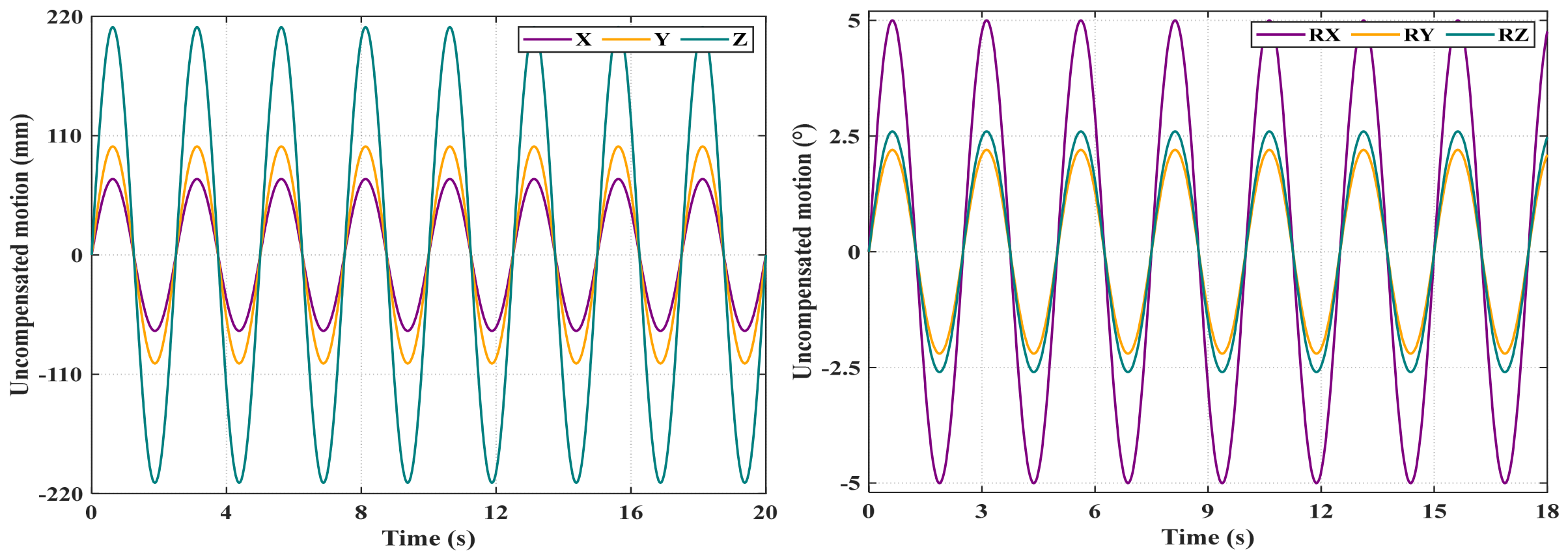
The 6-DOF sinusoidal excitation defined in Section 4.1 is adopted as the offline optimization condition. For each candidate parameter vector, the same $K_p$, $K_i$, and $\lambda$ values are assigned to the position loop FOPI controllers of the six actuator legs. The closed loop MATLAB/Simulink R2025b model is then evaluated over $0\le t\le T$ under the specified optimization condition. The resulting six leg-length tracking errors are substituted into Equation (25) to calculate $J\left(x\right)$, and a smaller objective function value indicates a better candidate solution. The optimization terminates when the maximum number of iterations is reached, after which the global-best solution is selected as the optimized position loop FOPI parameter vector: $x^{*} ={\left[K_p^{*},K_i^{*},{\lambda }^{*} \right]}^{\mathrm{T}}$. The final optimized parameter vector is $x^{*} ={\left[45, 0.048, 0.6 \right]}^{\mathrm{T}}$. The resulting parameters are subsequently used without further modification in the stability analysis and closed-loop performance tests.

To further illustrate the offline optimization process, the best position loop FOPI parameters and the corresponding best objective function values at several representative iterations are listed in

Table 1. The course of the optimization process for the selected iteration of the optimization algorithm.

$\mathit{q}$	${\mathit{K}}_{\mathit{p}}$	${\mathit{K}}_{\mathit{i}}$	$\mathit{\lambda }$	$\mathit{J}\left(\mathit{x}\right)$
1	43.59	0.039	0.55	95.5836
10	44.88	0.047	0.57	33.4979
25	44.59	0.046	0.59	6.8427
50	45	0.048	0.6	${10}^{-12}$
100	45	0.048	0.6	${10}^{-12}$
200	45	0.048	0.6	${10}^{-12}$
350	45	0.048	0.6	${10}^{-12}$

. The values reported at each selected iteration correspond to the best solution obtained from the beginning of the optimization up to that iteration, rather than to the average parameter values of the current population.

Based on the results presented in Table 1, it can be concluded that during the first 50 iterations, the optimization algorithm searched within the predefined bounds and obtained the optimal solution at the 50th iteration. The optimal solution remained unchanged during the subsequent iterations.

3.4.2. Comparative and Convergence Analysis of Optimization Algorithms

To evaluate whether TSO is suitable for the FOPI parameter-optimization problem considered in this study, additional comparisons with the WOA and ChOA were conducted. All three algorithms were used to optimize the same FOPI parameters of the position loop, namely $K_p$, $K_i$, and $\lambda$, using the same objective function, parameter bounds, population size, and maximum number of iterations [40]. The population size and the maximum number of iterations were set to 180 and 350, respectively. For WOA, the convergence coefficient $a$ was defined as $a\left(q\right)=2\left(1-{\displaystyle \frac{q}{q_{max}}}\right)$, so that $a$ decreases linearly from 2 to 0 during the iterative process [41,42]. For ChOA, the convergence coefficient $f$ was defined as $f\left(q\right)=2.5\left(1-{\displaystyle \frac{q}{q_{max}}}\right)$, and therefore decreases linearly from 2.5 to 0 during the optimization process. In the ChOA implementation used in this study, the same $f\left(q\right)$ schedule was adopted for the attacker, barrier, chaser, and driver individuals [43]. These coefficients are used to regulate the balance between global exploration in the early stage and local exploitation in the later stage. To account for the stochastic nature of the algorithms, each algorithm was independently executed 20 times under the same computing environment. 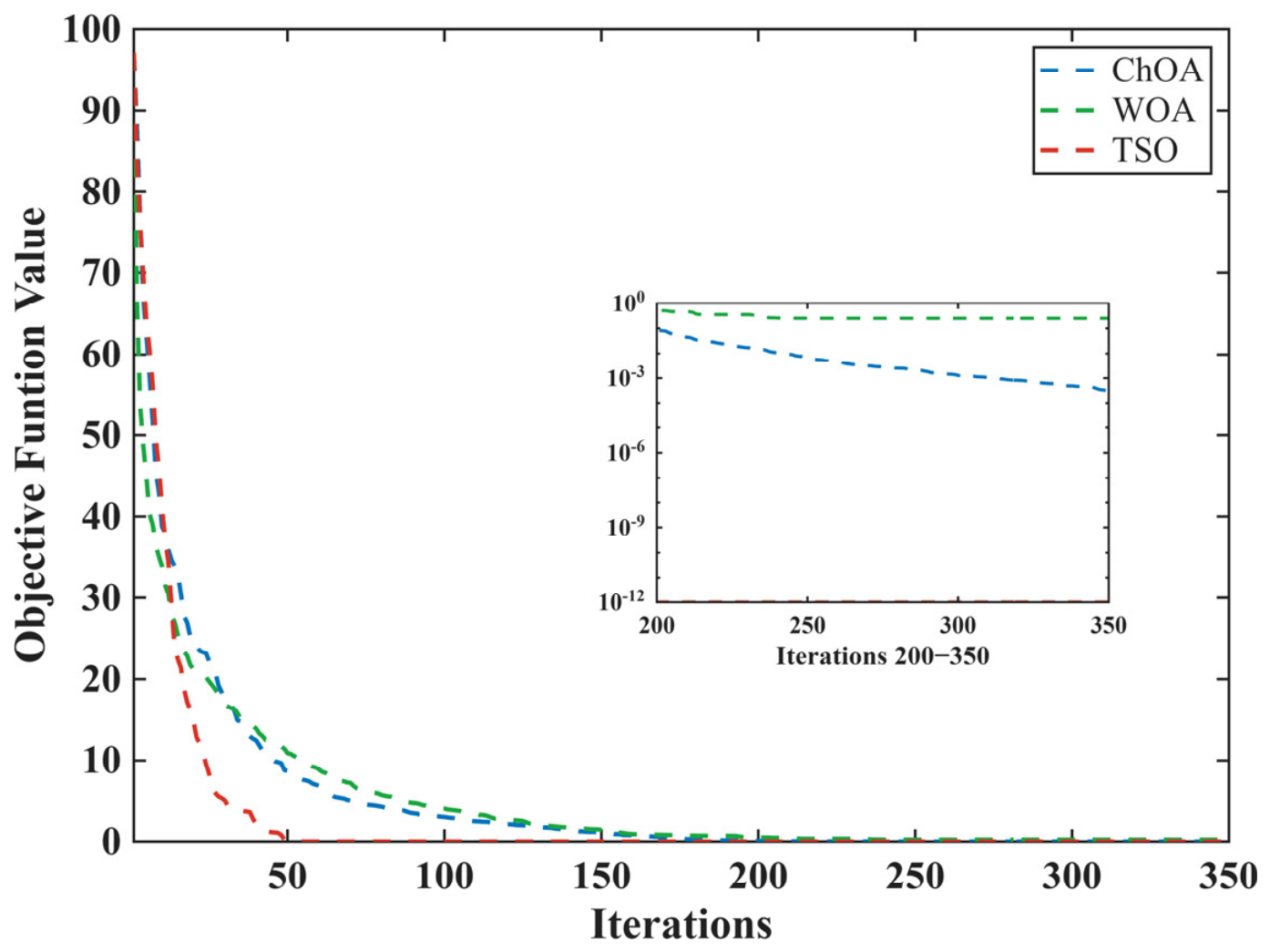Figure 7 illustrates the mean best-so-far objective function convergence curves of ChOA, WOA, and TSO over 20 independent runs.

For each run, the best objective-function value obtained up to the current iteration was recorded, and the corresponding values were then averaged over the 20 runs. As shown in Figure 7, all three algorithms gradually reduce the objective function value as the iteration proceeds, indicating that they are all capable of solving the position-loop FOPI parameter optimization problem. TSO exhibits the fastest overall convergence among the three algorithms. Although ChOA and WOA also show a rapid reduction in the objective function value during the early iterations, TSO enters the low objective value region earlier and approaches its final value after approximately 50 iterations. In contrast, ChOA and WOA require more iterations to approach their respective final solutions. The logarithmic inset for iterations 200–350 further shows that TSO maintains the lowest objective function value, whereas ChOA continues to improve gradually and WOA tends to remain at a relatively higher objective function level. These results indicate that TSO provides a favorable convergence rate and optimization performance for the FOPI parameter-tuning problem considered in this study.

3.5. Stability Analysis of the Cascaded FOPI Control Loops

According to the inverse-kinematics and transmission relationships, the reference rotor angular position is denoted as ${\theta }_m^{ref}$. In the position loop, the actual rotor angular position is ${\theta }_m$, and the position error is defined as:

$$e_p={\theta }_m^{ref}-{\theta }_m$$

(28)

The current-loop error is defined as:

$$e_{id}=i_d^{ref}-i_d , e_{iq}=i_q^{ref}-i_q$$

(29)

where $i_d^{ref}$ and $i_q^{ref}$ denote the d- and q-axis current references, and $i_d$ and $i_q$ are the corresponding actual currents.

The speed-loop error is defined as:

$$e_{\omega }={{\omega }_m^{ref}-\omega }_m$$

(30)

where ${\omega }_m^{ref}$ and ${\omega }_m$ are the reference and actual angular speeds, respectively.

The motor plant model with the load disturbance $T_L$ can be expressed as:

$${\mathsf{\Theta }}_m \left(s\right)=P_{pos}\left(s\right)\left(T_e\left(s\right)-T_L\left(s\right)\right)$$

(31)

where $P_{pos}\left(s\right)={\displaystyle \frac{1}{J{s}^2+Bs}}$, $P_{pos}\left(s\right)$ is the mechanical transfer function from torque to rotor position, and ${\mathsf{\Theta }}_m \left(s\right)$, $T_e\left(s\right)$, and $T_L\left(s\right)$ are the Laplace transforms of ${\theta }_m$, $T_e$, and $T_L$, respectively.

According to the Equation $\left(17\right)$, the position-loop parameters $K_{p\theta }$, $K_{i\theta }$, and ${\lambda }_{\theta }$ are determined through offline TSO-based optimization, whereas the current-loop and speed-loop parameters are fixed at their prescribed values. The transfer function of the triple-loop FOPI controller can be written in a unified form as:

$$C_k(s)=K_{pk}+K_{ik}{s}^{-{\lambda }_k}$$

(32)

where $k\in \left\{i,\omega ,\theta \right\},0{<\lambda }_k<1$, and $K_{pk}$, $K_{ik}$, and ${\lambda }_k$ are the proportional gain, integral gain, and integral order of the $k$-th loop, respectively.

(1)

Stability analysis of current loop

The transfer function of the current-loop plant is:

$$G_i(s)={\displaystyle \frac{K_c}{{\tau }_{i}s+1}}, K_c>0,{\tau }_i>0$$

(33)

where $K_c$ is the current-loop gain and ${\tau }_i$ is the current-loop time constant. Clearly, there are no right-half-plane poles.

For $\omega >0$, the frequency response of the $k$-th FOPI controller can be written as:

$$C_k\left(j\omega \right)=A_k\left(\omega \right)-j{B}_k\left(\omega \right)$$

(34)

where

$$A_k\left(\omega \right)=K_{pk}+K_{ik}{\omega }^{-{\lambda }_k}\cos {\displaystyle \frac{{\lambda }_k\pi }{2}}, B_k\left(\omega \right)=K_{ik}{\omega }^{-{\lambda }_k}\sin {\displaystyle \frac{{\lambda }_k\pi }{2}}$$

(35)

Because $K_{pk}>0, K_{ik}>0$, both $A_k\left(\omega \right)$ and $B_k\left(\omega \right)$ are positive for all $\omega >0$. The fractional orders adopted in this study are ${\lambda }_i=0.55$, ${\lambda }_{\omega }=0.5$, and ${\lambda }_{\theta }=0.6$.

Substituting Equation (34) into Equation (33) gives:

$$\mathrm{Im}\left[L_i\left(j\omega \right)\right]=-{\displaystyle \frac{K_c\left[{\tau }_i\omega A_i\left(\omega \right)+B_i\left(\omega \right)\right]}{1+{{\tau }_i^2\omega }^2}}<0, \omega >0$$

(36)

Therefore, the positive-frequency branch of the current-loop Nyquist locus remains strictly below the real axis over the entire frequency range and has no finite-frequency crossing of the negative real axis. The negative-frequency branch is its complex conjugate. The fractional-integral singularity at the origin is excluded using an indented Nyquist contour, because $0{<\lambda }_i<1$, its image connects the two frequency branches through the right half of the complex plane and does not pass through the critical point $-1+j0$. Since $L_i\left(s\right)$ has no right-half-plane poles, its complete Nyquist locus has no encirclement of $-1+j0$. Thus, according to the Nyquist criterion, the current loop is stable.

(2)

Stability analysis of speed loop

The transfer function of the speed-loop plant is:

$$G_{\omega }\left(s\right)={\displaystyle \frac{K_t}{J_m s+B_m }},K_t>0, J_m >0,B_m>0$$

(37)

where $K_t$ is the electromagnetic torque constant. This plant also has no right-half-plane poles.

According to Equation (34), the imaginary part of the speed-loop frequency response is:

$$\mathrm{Im}\left[L_{\omega }\left(j\omega \right)\right]=-{\displaystyle \frac{K_t\left[J_m\omega A_{\omega }\left(\omega \right)+B_m{B}_{\omega }\left(\omega \right)\right]}{B_m^2+J_m^2{\omega }^2}}<0, \omega >0$$

(38)

Hence, the positive-frequency Nyquist branch of the speed loop also remains strictly below the real axis and does not cross the negative real axis at any finite frequency. The origin singularity is treated using the same indented-contour argument as for the current loop. Because the speed-loop open-loop model has no right-half-plane poles and its complete Nyquist locus does not encircle $-1+j0$, the speed loop is stable. The load disturbance $T_L$ acts as an external disturbance input. It affects the forced response of the speed loop but does not appear in the characteristic equation $1+L_{\omega }\left(s\right)=0$. Therefore, it does not alter the closed-loop pole locations.

(3)

Stability analysis of position loop

The transfer function of the position-loop plant is:

$$G_{\theta }\left(s\right)={\displaystyle \frac{K_{\omega }}{s\left(1+T_{\omega }s\right)}}{, K}_{\omega }>0, T_{\omega } >0$$

(39)

where $K_{\omega }$ is the equivalent gain of the closed speed loop and $T_{\omega }$ is the position-loop time constant. This plant contains only a pole at the origin and left-half-plane poles.

The open-loop transfer function of the position loop is:

$$L_{\theta }\left(s\right)=C_{\theta }\left(s\right)G_{\theta }\left(s\right)$$

(40)

For $\omega >0$, the real and imaginary parts of the position-loop frequency response are:

$$\mathrm{Re}\left[L_{\theta }\left(j\omega \right)\right]=-{\displaystyle \frac{K_{\omega }\left[T_{\omega }\omega A_{\theta }\left(\omega \right)+B_{\theta }\left(\omega \right)\right]}{\omega \left(1+{T_{\omega }^2\omega }^2\right)}}<0, \mathrm{Im}\left[L_{\theta }\left(j\omega \right)\right]={\displaystyle \frac{K_{\omega }\left[T_{\omega }\omega B_{\theta }\left(\omega \right)-A_{\theta }\left(\omega \right)\right]}{\omega \left(1+{T_{\omega }^2\omega }^2\right)}}$$

(41)

The squared magnitude is:

$${\left|L_{\theta }\left(j\omega \right)\right|}^2={\displaystyle \frac{K_{\omega }^2\left[K_{p\theta }^2+2K_{p\theta }{K}_{i\theta }\cos \frac{{\lambda }_{\theta }\pi }{2}{\omega }^{-{\lambda }_{\theta }}+K_{i\theta }^2{\omega }^{-{2\lambda }_{\theta }}\right]}{{\omega }^2\left(1+{T_{\omega }^2\omega }^2\right)}}$$

(42)

The numerator of Equation (42) decreases with $\omega$, whereas its denominator increases strictly. Consequently, $\left|L_{\theta }\left(j\omega \right)\right|$ decreases strictly from infinity to zero as $\omega$ increases from zero to infinity. Therefore, there is one and only one gain-crossover frequency ${\omega }_{c\theta }$.

To determine the negative-real-axis crossing, define:

$$F_{\theta }\left(\omega \right)=T_{\omega }\omega B_{\theta }\left(\omega \right)-A_{\theta }\left(\omega \right)$$

(43)

For $0{<\lambda }_{\theta }<1$, direct differentiation of Equation (43) gives: $F_{\theta }^{\prime }\left(\omega \right)>0$. Moreover, $\underset{\omega \to 0^{+}}{\lim }{F}_{\theta }\left(\omega \right)=-\infty$, $\underset{\omega \to \infty }{\lim }{F}_{\theta }\left(\omega \right)=+\infty$. Therefore, $F_{\theta }\left(\omega \right)=0$ has a unique positive solution, denoted by ${\omega }_{\pi \theta }$. According to Equation (41), ${\omega }_{\pi \theta }$ is the unique frequency at which the position-loop Nyquist locus crosses the negative real axis.

The position loop has a unique gain-crossover frequency ${\omega }_{c\theta }$, and the adopted controller parameters give a positive phase margin at this frequency. Since the negative-real-axis crossing is unique, it follows that ${\omega }_{c\theta }<{\omega }_{\pi \theta }$.

Because $\left|L_{\theta }\left(j\omega \right)\right|$ decreases strictly with frequency,

$$\left|L_{\theta }\left(j{\omega }_{\pi \theta }\right)\right|<\left|L_{\theta }\left(j{\omega }_{c\theta }\right)\right|=1$$

(44)

Hence, the unique negative-real-axis crossing lies between $-1+j0$ and the origin. The pole at the origin is treated using an indented Nyquist contour. Because $1{<1+\lambda }_{\theta }<2$, the image of the indented contour does not cross the negative real axis or pass through the critical point $-1+j0$. Since the open-loop position model has no right-half-plane poles and the complete Nyquist locus does not encircle $-1+j0$, the position loop is stable according to the Nyquist criterion.

Under the assumed bandwidth separation ${\omega }_{c\theta }\ll {\omega }_{c\omega }\ll {\omega }_{ci}$, where ${\omega }_{c\theta }$, ${\omega }_{c\omega }$, and ${\omega }_{ci}$ denote the gain-crossover frequencies of the position, speed, and current loops, respectively, the preceding analysis supports the internal stability of the equivalent cascaded FOPI control system for the adopted controller parameters.

4. Simulation Results and Discussion

To verify the effectiveness of the proposed TSO-FOPI control algorithm for wave compensation of a Stewart platform, the simulation model of the Stewart platform and the actuators are established, as shown in Figure 8. The desired lengths of each leg of the Stewart platform, calculated from the ship motions, are used as the inputs to the leg controllers. Subsequently, the individual leg lengths are validated in a closed-loop system using the TSO-FOPI controller. Finally, the residual motions of the moving platform are calculated after controlling the legs, both with and without using the proposed controller. A detailed model is also developed in MATLAB/Simulink. The key parameters of the Stewart platform and controllers are listed in

Table 2. Stewart platform model and controller parameters used in the simulations.

Parameter	Values	Parameter	Values	Parameter	Values
R	0.4	Ld	0.006	Lq	0.006
Pn	4	$J_m$	0.014	$B_m$	0.008
$K_{p,pi}$	30	$K_{i,pi}$	0.05	$K_{p,fopi,p}$	45
$K_{i,fopi,p}$	0.048	${\lambda }_{fopi,p}$	0.6	$K_{p,fopi,s}$	60
$K_{i,fopi,s}$	0.01	${\lambda }_{fopi,s}$	0.5	$K_{p,fopi,c}$	72
$K_{i,fopi,c}$	0.035	${\lambda }_{fopi,c}$	0.55

. The objective of this study is to maintain the moving platform stationary with respect to the inertial frame. Accordingly, the compensation error is defined as the deviation of the moving platform’s position and orientation relative to the inertial frame.

The PI controller was employed as a conventional baseline controller. Its proportional and integral gains were determined through iterative manual tuning in the MATLAB/Simulink model. First, the integral gain was set to zero, and the proportional gain was gradually increased to obtain a sufficiently fast response without sustained oscillation. The integral gain was then increased to reduce the steady-state tracking error, followed by fine adjustment of both gains to achieve a compromise between tracking accuracy and response smoothness. The resulting parameters were $K_{p,pi}=30$ and $K_{i,pi}=0.05$. These parameters were kept unchanged in all subsequent simulation cases.

4.1. Control Performance Test

To evaluate the control performance of the proposed algorithm for a Stewart platform under 6-DOF disturbances (surge, sway, heave, roll, pitch, and yaw), the following sinusoidal signals are selected to simulate wave-induced motion disturbances: $x=0.07\sin (4/5\pi t), y=0.1\sin (4/5\pi t), z=0.21\sin (4/5\pi t), Rx=5\pi /180·\sin (4/5\pi t), Ry=2.2\pi /180·\sin (4/5\pi t), Rz=2.6\pi /180·\sin (4/5\pi t)$, as shown in Figure 9. The compensation errors of the three controllers are presented in Figure 10. To quantitatively evaluate the control performance, Equations (45) and (46) are used to compute the root-mean-square error (RMSE) of the residual pose compensation error and the root-mean-square error of the residual velocity error (VRMSE), respectively. These metrics are then used to assess the compensation accuracy and stability of the controllers. Since the objective of wave compensation is to keep the moving platform stationary with respect to the inertial frame, the ideal residual pose and velocity are all zero.

$$RMSE=\sqrt{{\displaystyle \frac{1}{N}}{\displaystyle \sum _{i=1}^N}{\left(t_i-0\right)}^2}$$

(45)

$$VRMSE=\sqrt{{\displaystyle \frac{1}{N}}{\displaystyle \sum _{i=1}^N}{\left(v_{t,i}-0\right)}^2}$$

(46)

where $v_{t,i}={\dot{t}}_i$, $t_i$ denotes the actual value of the $i$-th sample and $v_{t,i}$ denotes the actual velocity of the $i$-th sample.

According to Equations (45) and (46), under sinusoidal excitation, the PI controller yields an average translational error of 10.11 mm and an average rotational error of 0.31 deg. The corresponding average translational and rotational velocity errors are 36.48 mm/s and 1.88 deg/s. For the FOPI controller, the average translational and rotational errors are 6.86 mm and 0.19 deg, respectively, while the corresponding average translational and rotational velocity errors are 29.64 mm/s and 0.59 deg/s, respectively. For the TSO-FOPI controller, the average translational and rotational errors are 5.12 mm and 0.12 deg, respectively, the corresponding average translational and rotational velocity errors are 21.79 mm/s and 0.37 deg/s, respectively. These results indicate that the PI, FOPI, and TSO-FOPI controllers all deliver satisfactory control performance. However, the conventional PI controller relies on experience-based manual tuning, and once the parameters are fixed, they cannot be adjusted online according to real-time errors. Consequently, when the phase and amplitude of the sinusoidal input vary over time, the system may respond sluggishly, leading to relatively large tracking errors. In addition, due to the limited bandwidth of the PI controller, its ability to track sinusoidal signals is constrained, resulting in poorer compensation stability. As shown in Figure 10, noticeable overshoot and oscillations occur during the dynamic process. Compared with PI control, FOPI control introduces an additional tunable integral order, which enables partial decoupling between phase and gain, making the system more stable with a smoother dynamic response. Nevertheless, conventional FOPI tuning still relies on experience-based trial-and-error procedures and may be trapped in local optima, without guaranteeing a globally optimal solution. The TSO-FOPI controller adopts TSO, which mimics the spiral and parabolic foraging behaviors of tuna swarms, to globally optimize the initial FOPI parameters $K_p$, $K_i$, and $\lambda$. By iteratively updating the population positions, it searches the parameter space for the solution that minimizes the error. The effectiveness of the parameter optimization is further confirmed by the results in Figure 10.

4.2. Frequency Domain Condition Analysis

The typical excitation frequency range of a shipborne Stewart platform under wave disturbances spans from 10⁻² to 10⁰ Hz. To better illustrate the advantages of the proposed controller, a swept-frequency excitation is applied in Simulink in this section. For clarity, only the sweep signals in the translational x direction and the rotational Rz direction are considered, as shown in Figure 11a,d, that is $x=0.05\sin \left({\omega }_x\right) , Rz=5\sin \left({\omega }_{Rz}\right)$, where ${\omega }_x=2\pi f_{start}t+\pi \left(f_{end}-f_{start}\right)·t^2/50 , {\omega }_{Rz}=2\pi f_{start}t+\pi \left(f_{end}-f_{start}\right)·t^2/50 ,{ f}_{start}={10}^{-2} \mathrm{H}\mathrm{z} , { f}_{end}={10}^0 \mathrm{H}\mathrm{z}$. As can be observed in Figure 11b,e, the compensation errors of all three controllers increase as the excitation frequency rises. However, throughout the entire sweep frequency, the proposed TSO-FOPI controller consistently maintains the smallest error amplitude. It is further noted that, under practical sea conditions, the Stewart platform is not only excited by waves within the typical frequency range, but also affected by higher-frequency components introduced by actuator dynamics, structural inherent modes, and sensor noise. Therefore, the Power Spectral Density (PSD) of the compensation error is analyzed over the frequency band of 10⁻¹ to 10¹ Hz to provide a more stringent evaluation of the controller’s wideband anti-disturbance performance. The PSD is defined as $S_e\left(f\right)=\underset{T\to \infty }{\lim }{\displaystyle \frac{1}{T}}{\left|{\int }_0^{T}e\left(t\right)e^{-j2\pi ft}dt\right|}^2$, and its magnitude and distribution along the frequency axis can characterize the strength of the platform’s residual position vibration at different frequencies. From a frequency-domain perspective, the error power spectral density reflects the closed-loop system’s ability to suppress disturbances and measurement noise at different frequencies, as well as the extent of resonance peak amplification (peaking).

The PI controller has limited tuning freedom, making it difficult to balance disturbance suppression and stability margin at the same time, and it tends to show a rise in the spectrum or insufficient attenuation in higher-frequency ranges (10⁰ to 10¹ Hz). The FOPI controller introduces fractional-order characteristics, but without global optimization tuning, its parameter matching and robustness are still limited. As a result, relatively clear spectral peaks may remain, and the spectral magnitude in the 10⁰ to 10¹ Hz band can still be high. In contrast, TSO-FOPI benefits from the additional tunable freedom brought by the fractional-order term and performs global parameter tuning via the tuna swarm optimization algorithm, which helps achieve more reasonable closed-loop frequency-response characteristics and peak suppression. Meanwhile, it strengthens high-frequency attenuation and reduces the amplification of high-frequency measurement noise, leading to a lower error PSD level over the entire frequency range of interest. From the error PSD curves in Figure 11c,f, it can be seen that within 10⁻¹ to 10¹ Hz, which covers the typical operating band of the platform, the overall error spectra are relatively low for all three controllers. Among them, the PI controller yields the largest PSD magnitude, the FOPI controller reduces it to some extent, and the proposed TSO-FOPI controller remains at the lowest level across the band. When the frequency range is further extended toward 10⁰ to 10¹ Hz, the PI controller exhibits a clear rise in the error spectrum with pronounced peaks, and the FOPI controller is still noticeably higher than TSO-FOPI, whereas the TSO-FOPI spectrum stays at a low magnitude and decays faster as frequency increases.

These results indicate that the proposed control strategy can effectively suppress residual platform vibrations in the typical wave-excitation band and demonstrate better wideband disturbance-rejection performance against the introduced high-frequency disturbances, thereby significantly improving the position and attitude stability of the shipborne Stewart platform. Together with the previously reported time-domain compensation-error comparisons under random-wave excitation, the results further verify the overall vibration-suppression advantage of the TSO-FOPI controller under representative sea states and broadband disturbance conditions.

4.3. Time-Domain Response Analysis

Shipborne Stewart platforms are typically used for the transfer of personnel and cargo under sea state 4 conditions. To evaluate the control effectiveness of the controller designed in this paper on the platform’s 6-DOF motion under this sea state, the MATLAB Marine Systems Simulator (MSS) toolbox is adopted. Based on the JONSWAP spectrum and random wave motion theory, the wave excitation is generated and then converted into random disturbance inputs induced by ship motions. Figure 12 shows the 6-DOF random wave disturbance at sea state 4. The resulting disturbance signals cover all six DOFs of the platform, thereby providing a representative simulation scenario for validating the controller’s dynamic response under sea state 4. Meanwhile, to test the anti-disturbance capability of the control algorithm under sudden load changes, load forces and torques are applied according to the load characteristics of the moving platform. Specifically, the disturbance forces in the x, y, and z directions are $F_x = F_y = 1500 \mathrm{N} , F_z = 2500 + 2500\sin (2/3\pi t) \mathrm{N}$, and the disturbance torques in Rx, Ry, and Rz directions are $T_{Rx}=T_{Ry}=250\sin (2/3\pi t) \mathrm{N}·\mathrm{m} ,T_{Rz}=250 \mathrm{N}·\mathrm{m}$.

As shown in Figure 13, the PI algorithm can maintain a good control effect. However, with fixed parameters, it lacks adaptive adjustment capability against the broadband disturbances of random waves, leading to possible overshoot or oscillations. Compared with PI, the FOPI algorithm shows better tuning flexibility and thus exhibits stronger robustness to the nonlinear disturbances induced by random waves. However, due to the limitations of manual tuning, the FOPI algorithm may lead to the system being trapped in a local optimum. The TSO-FOPI controller utilizes TSO’s strong global search capability to identify better parameters, thereby enhancing the anti-disturbance performance of FOPI control. Furthermore, the compensation errors of the three control algorithms are similar regardless of load disturbances, indicating that they all possess strong anti-disturbance capability. To quantify the compensation capability of these three control algorithms for the platform under sea state 4, Equations (45) and (46) are used to calculate the RMSE and VRMSE of the residual pose and residual velocity, respectively. As listed in

Table 3. The compensation performance of different controllers.

Waves		X	Y	Z	RX	RY	RZ	XYZ	RXRYRZ
	PI	2.44 mm	2.78 mm	5.95 mm	0.09 deg	0.11 deg	0.19 deg	3.72 mm	0.13 deg
RMSE	FOPI	1.74 mm	1.93 mm	3.99 mm	0.02 deg	0.08 deg	0.13 deg	2.55 mm	0.08 deg
	TSO-FOPI	1.39 mm	1.44 mm	2.12 mm	0.02 deg	0.06 deg	0.07 deg	1.65 mm	0.05 deg
	PI	13.43 mm/s	15.05 mm/s	14.53 mm/s	2.7 deg/s	0.81 deg/s	1.68 deg/s	14.34 mm/s	1.73 deg/s
VRMSE	FOPI	10.47 mm/s	9.11 mm/s	10.41 mm/s	0.2 deg/s	0.71 deg/s	0.35 deg/s	10 mm/s	0.42 deg/s
	TSO-FOPI	8.35 mm/s	7.74 mm/s	7.36 mm/s	0.13 deg/s	0.45 deg/s	0.2 deg/s	7.82 mm/s	0.26 deg/s

Note: XYZ and RXRYRZ denote the arithmetic mean values of the corresponding indices in the X, Y, Z directions and the RX, RY, RZ directions, respectively.

, under random wave excitation, the PI controller yields an average translational error of 3.72 mm and an average rotational error of 0.13 deg. The corresponding average translational and rotational velocity errors are 14.34 mm/s and 1.73 deg/s, respectively. For the FOPI controller, the average translational and rotational errors are 2.55 mm and 0.08 deg, while the corresponding average translational and rotational velocity errors are 10.00 mm/s and 0.42 deg/s, respectively. For the TSO-FOPI controller, these values are reduced to 1.65 mm, 0.05 deg, 7.82 mm/s, and 0.26 deg/s, respectively. For each baseline controller, the percentage reductions in the mean translational and rotational indices are calculated separately, and the overall percentage improvement is obtained as their arithmetic mean, as defined in Equation (47). Accordingly, the proposed strategy reduces the average compensation error, based on the translational and rotational RMSE indices, by about 59$\%$ and 36.4$\%$, respectively, and improves the average compensation smoothness, evaluated using the corresponding VRMSE indices, by about 65$\%$ and 30.25$\%$, respectively.

$${\eta }_M={\displaystyle \frac{1}{2}}\left[{\displaystyle \frac{M_{T, \mathrm{base}}-M_{T, \mathrm{TSO}-\mathrm{FOPI}}}{M_{T, \mathrm{base}}}}+{\displaystyle \frac{M_{R, \mathrm{base}}-M_{R, \mathrm{TSO}-\mathrm{FOPI}}}{M_{R, \mathrm{base}}}}\right]\times 100\%$$

(47)

where $M$ denotes either the RMSE or VRMSE index, $M_T$ denotes the average translational error indices, and $M_R$ denotes the average rotational error indices. Only the dimensionless percentage reductions, rather than the translational and rotational quantities with different units, are averaged.

5. Conclusions

This paper proposes a TSO-FOPI triple-loop control strategy based on the tuna swarm optimization algorithm to address high-precision motion control challenges of a Stewart platform in complex marine environments. A dynamic model of the Stewart platform and a mathematical model of the PMSM actuator are developed. TSO is used to globally optimize the initial values of the core FOPI parameters, and the stability of the controller is verified. The coupling system of the mechanism and the actuator is established in MATLAB/Simulink. Simulation results show that the proposed strategy achieves anti-disturbance performance comparable to PI and FOPI control, while delivering better compensation accuracy and smoothness. Under swept-frequency excitation from 10⁻¹ to 10¹ Hz, power spectral density analysis of the compensation error indicates that the proposed controller, compared with PI and FOPI, can effectively suppress residual platform vibration in typical wave-excitation bands and shows better wideband anti-disturbance performance against the introduced high-frequency disturbances. Under random-wave excitation corresponding to a representative sea state 4 condition, the proposed strategy achieves lower translational and rotational RMSE and VRMSE values than both PI and FOPI control. Based on the averaged percentage reductions in the translational and rotational indices, the overall compensation error is reduced by about 59% and 36.4%, while the overall compensation smoothness is improved by about 65% and 30.25% compared with PI and FOPI control, respectively. These results demonstrate the effectiveness of the proposed strategy at the simulation level and indicate its potential for high-precision wave-compensation control. However, it should also be noted that, although the proposed control strategy performs well in terms of accuracy and robustness, the controller structure and the formulation of the offline optimization objective still involve manual design choices, which introduces dependence on experience and increases structural complexity. Additionally, although TSO is employed offline for controller parameter tuning, the execution time and real-time implementation performance of the resulting FOPI controller have not yet been quantitatively evaluated, particularly with respect to the implementation of the fractional-order operators. Future work will explore parameter self-adaptation mechanisms and structure-simplification strategies to reduce reliance on manual tuning and to improve portability and real-time performance in practical engineering applications. Meanwhile, by combining hardware-in-the-loop simulation and sea-trial dynamic tests, the reliability of the proposed strategy and its engineering applicability in real marine disturbance environments can be further validated.