Article

Dynamic Parameter Identification of a Lower-Limb Exoskeleton Using RLS–AGWO
1
School of Mechanical Engineering, Jiangsu University of Technology (JSUT), Changzhou 213001, China
2
School of Cyber Science and Engineering, Nanjing University of Science and Technology (NJUST), Nanjing 210094, China
*
Author to whom correspondence should be addressed.
Actuators 2026, 15(8), 447; https://doi.org/10.3390/act15080447
Submission received: 20 June 2026 / Revised: 2 August 2026 / Accepted: 6 August 2026 / Published: 17 August 2026

Abstract

Accurate dynamic parameters are required for model-based control of lower-limb exoskeletons, but limited excitation, transmission friction, and assembly-dependent uncertainty can degrade conventional estimates. This study examines a two-stage method that combines recursive least squares (RLS) with an adaptive grey wolf optimizer (AGWO). Offline RLS tracks the base-parameter trajectory and expands its post-convergence extrema to construct a finite search space; a non-smooth friction severity index then modulates the GWO convergence schedule. The method was evaluated on a pedestal-mounted, single-degree-of-freedom hip mechanism using a 5 s calibration trajectory and a separate 7 s validation trajectory. Deterministic least squares (LS) and bound-constrained least squares (BCLS) were compared with standard PSO, RLS–PSO, RLS–GA, RLS–GWO, and RLS–AGWO. Each stochastic method used a population of 30, with 80 iterations (2400 fitness evaluations) and 30 independent seeds. On the independent trajectory, BCLS obtained an RMSE of 0.1152 Nm. Median validation RMSEs were 0.1152, 0.1152, 0.1562, and 0.1516 Nm for RLS–PSO, RLS–GA, RLS–GWO, and RLS–AGWO, respectively. Thus, the adaptive schedule improved median GWO error by 3.0%, but deterministic BCLS was both more accurate and faster for the present linear-in-parameters model. AGWO is therefore not mathematically necessary for the current convex objective; its potential advantage should be tested with genuinely nonlinear friction parameterizations. The conclusions remain limited to a single-axis pedestal experiment and do not establish performance during human-worn gait.

1. Introduction

Lower-limb exoskeletons are being developed for load assistance, mobility support, gait rehabilitation, and quantitative human–robot interaction research [1,2,3,4]. Their controllers must generate useful assistance without masking the wearer’s intent or introducing parasitic interaction torque. This requirement makes model fidelity especially important: errors in inertia, gravity, and friction compensation are transmitted directly to the human–device interface. Accurate dynamic parameter identification therefore supports feedforward compensation, impedance control, interaction-force estimation, and adaptive compliant control [5,6,7].
Three routes are commonly used to obtain mechanical parameters. Manufacturer or CAD values are convenient, but they do not fully represent custom links, cables, fasteners, transmission losses, and the mass distribution of a wearer–device assembly. Direct measurement can isolate individual quantities, although it requires disassembly or dedicated tests and does not necessarily capture parameters under operating conditions. Data-driven dynamic identification instead estimates a minimal set of base-parameter combinations from measured motion and torque [8]. Its accuracy depends on excitation quality, regressor conditioning, signal differentiation, and the ability of the model to represent friction and compliance [9,10,11].
Batch least squares (LS) remains attractive because robot dynamics can often be written linearly in the base parameters. Recursive least squares (RLS) additionally tracks slow variation and can support online or repeated calibration. Nevertheless, measurement noise, collinearity among regressor columns, limited joint motion, and outliers can amplify uncertainty or yield estimates that violate physical expectations. Hybrid and robust LS methods, data weighting, nonlinear friction separation, and Kalman-smoothing formulations have consequently been investigated [12,13,14,15]. These methods improve numerical robustness, but reliable excitation and physically meaningful constraints remain central to parameter interpretation.
For exoskeletons, RLS-derived bounds have previously been combined with particle swarm optimization (RLS–PSO) and genetic algorithms (RLS–GA) [16,17]. Related work has used improved beetle-swarm and hybrid evolutionary algorithms for lower-limb exoskeletons and manipulators [18,19,20]. In parallel, recent robot-identification studies have emphasized deterministic or hybrid estimators that explicitly address weighting, physical feasibility, and nonlinear friction separation [12,13,14]. Such methods provide reproducible solutions and directly address feasibility or noise structure; population methods are potentially more flexible when the parameterization becomes genuinely nonlinear, discontinuous, or mixed discrete–continuous, but they require repeated runs and carefully equalized evaluation budgets. Collectively, these studies suggest that recursive estimation can supply useful prior ranges while a bounded second stage performs refinement. However, most population search schedules are chosen from generic optimization practice and are not adjusted according to a measured property of the electromechanical system.
The grey wolf optimizer (GWO) maintains three leaders and updates the remaining candidates through a transition from exploration to exploitation [21]. Nonlinear convergence schedules can improve performance on engineering problems [22], and GWO variants have been applied to hydraulic-actuator identification and robot calibration [23,24]. The unresolved question addressed here is whether a friction-related quantity extracted from the identification record can be used to adjust this schedule while RLS restricts the search to a data-supported domain. Importantly, for a fixed regressor, the adopted model is linear in the base-parameter vector; the role of AGWO is therefore to enforce and explore the RLS-informed bounded domain, not to replace the analytical LS solution of an unconstrained calibration problem.
The present formulation contributes an RLS-derived finite parameter domain and a non-smooth friction severity index (NFSI) that adapts the GWO convergence schedule using the estimated Coulomb friction contribution. The revised evaluation adds a deterministic bound-constrained least squares baseline, bounded standard GWO as an ablation, 30 independent runs under a common evaluation budget, sensitivity analyses, and a separate motion trajectory for validation. The experimental scope remains deliberately limited to a pedestal-mounted single-axis mechanism; it does not represent human-worn gait.

2. Dynamic Model and Linear Parameterization

2.1. Exoskeleton Configuration

The active power-assist hip exoskeleton (APHE) is shown in Figure 1. The platform comprises trunk, thigh, shank, and foot modules. The hip is actuated by a brushless DC motor coupled to a 156:1 planetary gearhead, and an output-shaft torque sensor measures the transmitted joint torque [17]. The archived experimental record identifies the drive type, reduction ratio, output torque sensing location, and 100 Hz acquisition rate, but it does not retain the motor power rating, encoder resolution, torque sensor range or accuracy, controller model, or real-time hardware. These unavailable specifications limit exact replication and are therefore not inferred here. During identification, the trunk and contralateral lower-limb assembly were secured to a rigid pedestal, while the tested leg was free to swing in the sagittal plane. The knee and ankle were mechanically locked so that the moving assembly could be treated as one rigid link. Accordingly, the tested device was a pedestal-mounted single-axis hip mechanism, not an exoskeleton operating during worn gait. The person in Figure 1 documents the physical fit of the platform only; no human-derived kinematic or torque data from that photograph entered the identification analysis. Written consent to publish the anonymized photograph was obtained.
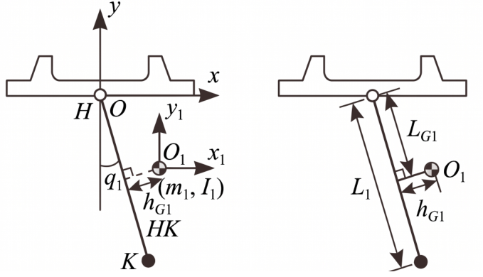
With the trunk fixed, the moving leg is represented in the sagittal plane by the single-link model in Figure 2. The generalized coordinate is the hip angle q 1 , measured counterclockwise from the vertically downward configuration. The equivalent link has mass m t , centroidal moment of inertia I t , and center-of-mass offsets L G t and h G t in the adopted coordinate convention. This reduction assumes rigid links, locked distal joints, a fixed hip axis, and negligible out-of-plane motion. Transmission friction is retained explicitly, whereas structural flexibility, backlash hysteresis, and human voluntary torque are absorbed into the residual term.
Using the Lagrange formulation, the rigid-body contribution to the hip torque is
T h = I t + m t L G t 2 + h G t 2 q ¨ 1 + m t g L G t sin q 1 + h G t cos q 1 ,
where g is gravitational acceleration. A Coulomb-plus-viscous model represents the joint friction:
T f = f c sgn ( q ˙ 1 ) + f v q ˙ 1 ,
where f c and f v are the Coulomb- and viscous-friction coefficients, respectively. Friction compensation is important in precision robot tracking and identification [14,25].

2.2. Linear Regression Form

Define the base parameters
M x t = m t L G t , M y t = m t h G t , J t = I t + m t L G t 2 + h G t 2 .
The measured motor-side torque can then be written as
T m ( k ) = H ( k ) X + ε ( k ) ,
with
X = M x t M y t J t f c f v T ,
H ( k ) = g sin q 1 ( k ) g cos q 1 ( k ) q ¨ 1 ( k ) sgn ( q ˙ 1 ( k ) ) q ˙ 1 ( k ) .
The residual ε ( k ) aggregates measurement noise and dynamics not represented by Equations (1) and (2). The five elements of X are base-parameter combinations rather than independently identifiable anatomical or CAD quantities. Identifiability requires the stacked regressor to have sufficient column rank and acceptable conditioning. The compound harmonic excitation used below changes position, acceleration, velocity magnitude, and velocity sign so that the gravity, inertia, Coulomb friction, and viscous-friction columns are activated within one record.

3. RLS–AGWO Identification Method

3.1. RLS-Based Bounded Search Space

RLS is first applied offline to track the variation of the base-parameter estimates. With forgetting factor λ , gain vector K ( k ) , and covariance matrix P ( k ) , the update is [26]
K ( k ) = P ( k 1 ) H T ( k ) λ + H ( k ) P ( k 1 ) H T ( k ) 1 ,
X ^ ( k ) = X ^ ( k 1 ) + K ( k ) T m ( k ) H ( k ) X ^ ( k 1 ) ,
P ( k ) = λ 1 I K ( k ) H ( k ) P ( k 1 ) .
The implementation uses λ = 0.98 , P ( 0 ) = 10 4 I , and X ^ ( 0 ) = 0 . The first 1.0 s of the RLS trajectory is treated as a burn-in interval and excluded before bound extraction. Componentwise minima and maxima of the retained trajectory are expanded by 10% of their span to form the lower and upper bounds L and U . If a mechanically required sign constraint is stricter than an RLS-derived limit, the mechanical constraint takes precedence. The 10% value follows the preceding RLS–PSO and RLS–GA workflow [16,17] and was evaluated against margins of 0, 5%, 20%, and 30%. The sensitivity analysis in Section 4.5 shows that no single margin dominates every seed; margins above 10% increased median validation error, whereas 0–10% remained in the lowest-error group. We therefore retain 10% as a conservative expansion that accommodates post-convergence variation without the wider domains produced by 20–30%. This procedure converts an unbounded search into a finite problem supported by the observed parameter trajectory.

3.2. Physics-Informed Adaptive Convergence Factor

Let H f denote the column of the stacked regressor associated with sgn ( q ˙ 1 ) , and let f ^ c , RLS be the RLS mean estimate of the Coulomb coefficient. The proposed NFSI is
γ = max H f f ^ c , RLS max T m + ϵ T ,
where ϵ T is a small positive number that prevents division by zero. This dimensionless ratio estimates the maximum share of measured torque associated with the discontinuous Coulomb term. It is used as a scheduling indicator rather than as a direct measurement of objective-function curvature. The GWO convergence factor is then defined as
a ( g , γ ) = 2 1 g G μ ( γ ) ,
μ ( γ ) = μ base + κ exp ( γ ) ,
where g is the current iteration, G is the maximum number of iterations, μ base is a baseline exponent, and κ is a sensitivity gain. Both hyperparameters are selected once before the comparison and held fixed throughout the AGWO run. For 0 < g / G < 1 , increasing μ keeps a closer to its upper value for longer and shifts the rapid decrease toward the end of the run. The intended effect is an extended exploration phase followed by a shorter exploitation phase when the estimated discontinuous-friction contribution is large.
For a candidate parameter vector X i , the fitness is the torque RMSE
J ( X i ) = 1 K k = 1 K T m ( k ) H ( k ) X i 2 .
The three best candidates are assigned the α , β , and δ leader roles. For leader { α , β , δ } , the update is [21]
A = 2 a r 1 , a , C = 2 r 2 , ,
D = C X X i , Y = X A D ,
X i ( g + 1 ) = clip [ L , U ] Y α + Y β + Y δ 3 ,
where ⊙ denotes componentwise multiplication and every element of r 1 , and r 2 , is sampled independently from U ( 0 , 1 ) . Boundary projection is applied after every update. With d = 5 parameters, K samples, N candidates, and G iterations, the dominant fitness evaluation cost is O ( G N K d ) .

3.3. Relation to Deterministic Bound-Constrained Least Squares

For the model used in this study, H is fixed after signal processing and the unknown vector enters linearly. Equation (13) is therefore equivalent to the convex quadratic program
X ^ BCLS = arg min L X U T m H X 2 2 .
A deterministic active-set, trust-region-reflective, or quadratic-programming solver can solve Equation (17) without stochastic initialization. AGWO is consequently not necessary to solve the present linear-in-parameters problem. Its rationale here is narrower: it preserves continuity with earlier RLS–population search calibration frameworks, demonstrates a system-dependent schedule within the same bounded domain, and provides a structure that can later accommodate genuinely nonlinear friction laws or mixed constraints. Section 4 reports BCLS directly and uses bounded standard GWO as an ablation baseline so that the adaptive schedule is not credited for benefits produced solely by RLS bounds. Table 1 presents the compact pseudocode of the proposed RLS–AGWO procedure.

4. Experimental Validation and Results

4.1. Platform, Excitation, and Data Acquisition

The APHE was mounted on a rigid pedestal in the configuration described in Section 2.1. The trunk and contralateral assembly were fixed, the tested leg was suspended, and the locked knee and ankle restricted the motion to one hip degree of freedom. The protocol comprised five stages: (1) execute the calibration motion and synchronously record joint angle and output torque; (2) filter the angle and obtain velocity and acceleration; (3) run offline RLS, discard the initial transient, and construct the bounds; (4) fit every estimator on the calibration record; and (5) evaluate the fixed parameter estimates on an independently recorded validation motion. The calibration reference was
q 1 , ref ( t ) = 60 + 30 sin ( π t ) + 15 cos ( 2 π t ) , 0 t < 5 s .
This compound trajectory combines 0.5 and 1 Hz components and repeatedly reverses the direction of motion, thereby exciting the gravity, inertia, and friction terms. A second record used the distinct reference
q 1 , val ( t ) = 48 + 20 sin ( 0.7 π t ) + 12 cos ( 1.7 π t ) + 5 sin ( 2.6 π t ) , 0 t < 7 s ,
which changes the offset, amplitudes, frequencies, duration, and reversal pattern. Angle and torque were sampled synchronously at 100 Hz, yielding 500 calibration samples and 700 validation samples. A fourth-order 15 Hz zero-phase Butterworth filter was applied to the angle before central finite-difference calculation of velocity and acceleration. Forward–backward filtering introduces no net phase lag but is suitable only for offline processing. Because differentiation amplifies high-frequency noise, the first and last 0.2 s were excluded, leaving 460 and 660 samples. The highest commanded validation component was 1.3 Hz, well below the 15 Hz cutoff and the 50 Hz Nyquist frequency. Section 4.5 reports the completed cutoff sensitivity analysis.
Table 2 gives the complete settings used for the revised comparison. All stochastic methods used 30 candidates for 80 iterations and therefore 2400 fitness evaluations per run. Thirty independently seeded runs were performed, and every method was evaluated on exactly the same calibration and validation arrays. The fixed 80-iteration budget was the stopping rule; no tolerance-based early stopping was used.

4.2. Evaluation Metrics and Comparison Protocol

Because the exact physical parameters of the assembled exoskeleton system are unavailable, identification quality was evaluated in the torque domain. For each method, the parameter vector fitted on the calibration record was held fixed and substituted into either the calibration or validation regressor to obtain T est ( k ) = H ( k ) X ^ . The signed residual is
T error ( k ) = T m ( k ) T est ( k ) ,
and the principal quantitative metric is
RMSE = 1 K k = 1 K T error 2 ( k ) .
The comparison includes unconstrained LS, deterministic BCLS, standard PSO, RLS–PSO, RLS–GA, bounded standard GWO, and RLS–AGWO. Training RMSE quantifies fitting on the calibration record, whereas validation RMSE is computed only on the independent trajectory. For stochastic methods, we report mean ± standard deviation (SD), median, interquartile range (IQR), and wall-clock runtime over 30 runs. The validation torque trace, signed residual, repeated-run distribution, and median/IQR convergence histories provide complementary views.

4.3. Independent-Trajectory Validation and Repeated-Run Statistics

Table 3 reports the independent-trajectory results. LS and BCLS produced the same feasible solution for this record, with calibration and validation RMSEs of 0.1419 and 0.1152 N m, respectively. The RLS-bounded PSO and GA distributions were concentrated near that deterministic optimum. Relative to bounded standard GWO, the adaptive schedule reduced median validation RMSE from 0.1562 to 0.1516 N m (3.0%). This ablation supports a modest schedule effect, not general superiority of AGWO. BCLS remained approximately 24.0% more accurate than median RLS–AGWO and was orders of magnitude faster.

4.4. Residual and Convergence Behavior

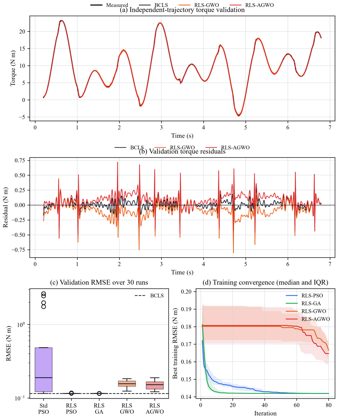
Figure 3a,b show that all three displayed fits follow the independent torque profile, but BCLS has the narrowest residual envelope. The largest excursions occur near direction reversals, consistent with the discontinuous Coulomb regressor and with differentiation sensitivity at sharp changes. The residual curves are not claimed to be white; that would require separate correlation and spectral tests.
Figure 3c exposes the instability hidden by a single seed: standard PSO has several high-error runs, while RLS–PSO and RLS–GA remain tightly clustered near BCLS. Figure 3d shows that PSO and GA reach low training error early, whereas GWO and AGWO improve mainly late in the run. AGWO has a lower final median than GWO, but their IQR bands overlap. Runtime differences should be interpreted as implementation-specific, although all population methods used an equal number of objective evaluations.

4.5. Parameter Estimates and Sensitivity Analysis

Table 4 reports the nominal reference values for the experimental apparatus and the estimates associated with BCLS and the median validation run of each RLS-bounded stochastic method. All methods recover the gravity and inertia combinations closely. The largest relative discrepancy occurs in Coulomb friction, which is expected because its regressor changes sign abruptly and is most affected by velocity estimation near zero crossings.
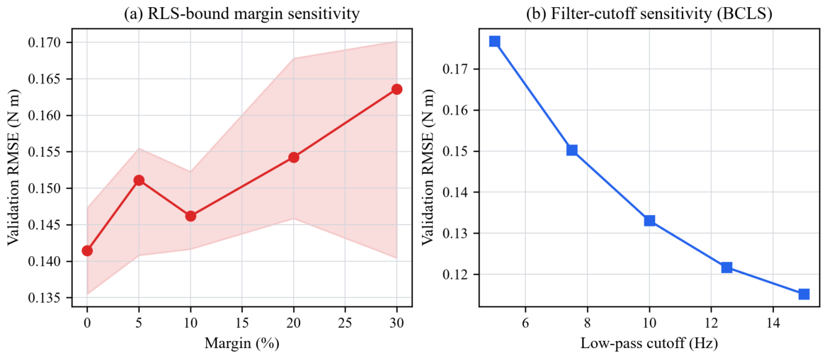
In Figure 4a, the median validation RMSEs for margins of 0, 5%, 10%, 20%, and 30% were 0.1414, 0.1511, 0.1462, 0.1542, and 0.1636 N m, respectively. The overlapping IQRs show that the precise ranking is seed-dependent; nevertheless, margins wider than 10% increased the median error, supporting the retained 10% compromise. Figure 4b shows BCLS validation RMSE decreasing from 0.1767 to 0.1152 N m as the cutoff increases from 5 to 15 Hz. This confirms that numerical differentiation materially affects identification, particularly the acceleration column, and motivates reporting the complete signal-processing chain rather than treating the cutoff as innocuous.

5. Discussion

5.1. Interpretation and Relation to Prior Work

The results extend the RLS-bounding strategy previously used with PSO and GA [16,17]. RLS supplies a compact domain inferred from the post-transient parameter trajectory. The repeated-run comparison shows why this prior is useful: standard PSO has a wide validation-error distribution, whereas RLS–PSO and RLS–GA converge consistently near the deterministic optimum. The bound-margin analysis also shows a trade-off. Too narrow a domain risks excluding plausible values, but unnecessarily wide bounds increase the stochastic search burden.
The GWO ablation isolates the adaptive schedule from the RLS bounds. Its 3.0% median improvement is measurable but modest, and overlapping dispersion prevents a broad superiority claim. More importantly, once H is fixed, Equation (13) is convex in the unknown vector: non-smoothness in sgn ( q ˙ 1 ) concerns measured velocity, not X . The BCLS result confirms the reviewer’s mathematical point and gives the most defensible solution for this model. AGWO is retained as a methodological bridge to future formulations with nonlinear friction, hysteresis, unknown breakpoints, or mixed constraints, where analytical linear least squares no longer applies.
The separate trajectory changes the motion spectrum and reversal pattern, so its RMSE is an out-of-sample validation measure rather than same-record fitting error. However, both records come from the same single-axis pedestal configuration and signal-processing pipeline. The result therefore supports transfer between two motions of this apparatus; it does not establish cross-device, human-worn, or clinical generalization.

5.2. Potential Applications

The identified base parameters can be embedded in computed-torque, gravity-feedforward, impedance, or sliding-mode controllers. More accurate torque reconstruction can reduce the corrective burden on a feedback loop, although the present offline experiment does not test closed-loop assistance. The method is also compatible with periodic automatic calibration: an exoskeleton could execute a short unloaded excitation, update its RLS bounds, and solve the bounded problem before operation. For the present linear model, BCLS is the recommended solver; population search becomes relevant only after the parameterization is extended beyond convex linear constraints.

5.3. Limitations and Future Work

Several limitations define the next research steps. First, the data cover one pedestal-mounted degree of freedom, two short trajectories, and one sensing/noise condition. They do not include multi-joint coupling, changing payloads, unrestricted human motion, or inter-participant variability. Future work should use leave-one-trajectory-out testing across speeds and amplitudes, then progress to ethically approved human-worn multi-joint experiments.
Second, although 30 seeds, equal evaluation budgets, runtimes, a GWO ablation, and two sensitivity studies are now reported, optimizer hyperparameters were held fixed. A fuller design should vary the RLS forgetting factor, population size, μ base , and κ and report formal paired uncertainty estimates. Third, the Coulomb-plus-viscous model cannot represent stiction, Stribeck behavior, asymmetry, temperature dependence, or backlash hysteresis. Those nonlinearities would provide a stronger motivation for population search but would also require broader independent validation. Finally, real-time use requires profiling on the target controller; the present results support offline or periodic calibration only.

6. Conclusions

This study evaluated a two-stage RLS–AGWO identification framework under a reproducible calibration/validation protocol. Thirty independent seeds and equal 2400-evaluation budgets showed that RLS bounds greatly reduced PSO and GA dispersion. The adaptive schedule reduced median validation RMSE from 0.1562 N m for bounded GWO to 0.1516 N m for RLS–AGWO, a 3.0% improvement. Nevertheless, deterministic BCLS achieved 0.1152 N m with substantially less computation and is the appropriate choice for the current convex linear-in-parameters problem. The useful conclusion is therefore not that AGWO replaces least squares, but that RLS-informed bounds and system-dependent scheduling form a testable framework for future nonlinear models. The evidence is limited to two trajectories of a single-axis pedestal apparatus and does not establish human-worn or real-time-control performance.

Author Contributions

Conceptualization and methodology, W.S.; validation and formal analysis, L.D.; investigation and data curation, L.D.; writing—original draft preparation, W.S.; writing—review and editing, Y.C.; supervision and theoretical guidance, T.G.; resources, T.G. All authors have read and agreed to the published version of the manuscript.

Funding

This research was funded by the Natural Science Foundation of Jiangsu Province under grants BK20251083 and BK20241491, and the National Natural Science Foundation of China (52375101).

Institutional Review Board Statement

Not applicable because no human-derived measurements were used in the parameter-identification dataset.

Informed Consent Statement

Written informed consent was obtained from the individual shown in Figure 1 for publication of the anonymized photograph.

Data Availability Statement

The calibration and independent-validation records, repeated-run results, sensitivity results, and reproduction code are included in the accompanying source archive.

Conflicts of Interest

The authors declare no conflicts of interest.

Abbreviations

The following abbreviations are used in this manuscript:
AGWOAdaptive grey wolf optimizer
APHEActive power-assist hip exoskeleton
GAGenetic algorithm
GWOGrey wolf optimizer
LSLeast squares
NFSINon-smooth friction severity index
PSOParticle swarm optimization
RLSRecursive least squares
RMSERoot-mean-square error

References

  1. Shushtari, M.; Arami, A. Human–Exoskeleton Interaction Force Estimation in Indego Exoskeleton. Robotics 2023, 12, 66. [Google Scholar] [CrossRef] [Scilit]
  2. Firouzi, V.; Seyfarth, A.; Song, S.; von Stryk, O.; Ahmad Sharbafi, M. Biomechanical Models in the Lower-Limb Exoskeletons Development: A Review. J. Neuroeng. Rehabil. 2025, 22, 12. [Google Scholar] [CrossRef] [Scilit] [PubMed]
  3. Hasan, S.K.; Alam, N. Comprehensive Comparative Analysis of Lower Limb Exoskeleton Research: Control, Design, and Application. Actuators 2025, 14, 342. [Google Scholar] [CrossRef] [Scilit]
  4. Vélez-Guerrero, E.; Salazar, J.A.; Rodríguez-León, J.F. Artificial Intelligence-Based Wearable Robotic Exoskeletons for Rehabilitation: A Review. Sensors 2021, 21, 2146. [Google Scholar] [CrossRef] [Scilit] [PubMed]
  5. Wu, J.; Wang, J.; You, Z. An Overview of Dynamic Parameter Identification of Robots. Robot. Comput.-Integr. Manuf. 2010, 26, 414–419. [Google Scholar] [CrossRef] [Scilit]
  6. Chen, H.; Guo, Y.; Zhang, Z. Parameter Identification and Adaptive Compliant Control of Rehabilitation Exoskeleton Based on Multiple Sensors. Measurement 2020, 159, 107765. [Google Scholar] [CrossRef] [Scilit]
  7. Li, Y.; Guan, X.; Li, W.; Penzlin, B.; Liu, K.; Yang, Z.; Liu, B.; Leonhardt, S.; Ji, L. Dynamic Parameter Identification of a Human-Exoskeleton System With the Motor Torque Data. IEEE Trans. Med. Robot. Bionics 2022, 4, 206–218. [Google Scholar] [CrossRef] [Scilit]
  8. Gautier, M.; Khalil, W. Direct Calculation of Minimum Set of Inertial Parameters of Serial Robots. IEEE Trans. Robot. Autom. 1990, 6, 368–373. [Google Scholar] [CrossRef] [Scilit]
  9. Calafiore, G.; Indri, M.; Bona, B. Robot Dynamic Calibration: Optimal Excitation Trajectories and Experimental Parameter Estimation. J. Robot. Syst. 2001, 18, 55–68. [Google Scholar] [CrossRef]
  10. Tian, H.; Huber, M.; Mower, C.E.; Han, Z.; Li, C.; Duan, X.; Bergeles, C. Excitation Trajectory Optimization for Dynamic Parameter Identification Using Virtual Constraints in Hands-on Robotic System. In Proceedings of the 2024 IEEE International Conference on Robotics and Automation (ICRA), Yokohama, Japan, 13–17 May 2024; pp. 11605–11611. [Google Scholar] [CrossRef] [Scilit]
  11. Luo, R.; Yuan, J.; Hu, Z.; Du, L.; Bao, S.; Zhou, M. Lie-Theory-Based Dynamic Model Identification of Serial Robots Considering Nonlinear Friction and Optimal Excitation Trajectory. Robotica 2024, 42, 3552–3569. [Google Scholar] [CrossRef] [Scilit]
  12. Huang, Y.; Ke, J.; Zhang, X.; Ota, J. Dynamic Parameter Identification of Serial Robots Using a Hybrid Approach. IEEE Trans. Robot. 2023, 39, 1607–1621. [Google Scholar] [CrossRef] [Scilit]
  13. Xu, T.; Tuo, H.; Wang, C.; Zhang, Z. Robot Dynamic Identification Based on Data Weighting Protection and Nonlinear Friction Separation. IEEE/ASME Trans. Mechatron. 2025, 30, 5508–5519. [Google Scholar] [CrossRef] [Scilit]
  14. Dong, J.; Xu, J.; Zhou, Q.; Zhu, J.; Yu, L. Dynamic Identification of Industrial Robot Based on Nonlinear Friction Model and LS-SOS Algorithm. IEEE Trans. Instrum. Meas. 2021, 70, 7504512. [Google Scholar] [CrossRef] [Scilit]
  15. Ljung, L. System Identification: Theory for the User, 2nd ed.; Prentice Hall: Upper Saddle River, NJ, USA, 1999. [Google Scholar]
  16. Zha, F.; Sheng, W.; Guo, W.; Qiu, S.; Deng, J.; Wang, X. Dynamic Parameter Identification of a Lower Extremity Exoskeleton Using RLS-PSO. Appl. Sci. 2019, 9, 324. [Google Scholar] [CrossRef] [Scilit]
  17. Sheng, W.; Cao, Y.; Ghalichi, F.; Ding, L.; Gao, T. Dynamic Parameter Identification of a Hip Exoskeleton Using RLS-GA. Actuators 2026, 15, 106. [Google Scholar] [CrossRef] [Scilit]
  18. Zhang, P.; Zhang, J. Lower Limb Exoskeleton Robots’ Dynamics Parameters Identification Based on Improved Beetle Swarm Optimization Algorithm. Robotica 2022, 40, 2716–2731. [Google Scholar] [CrossRef] [Scilit]
  19. Lu, Z.; Wei, C.; Ni, D.; Bi, J.; Wang, Q.; Li, Y. Dynamic Parameter Identification of Modular Robot Manipulators Based on Hybrid Optimization Strategy: Genetic Algorithm and Least Squares Method. Soft Comput. 2024, 28, 9991–10005. [Google Scholar] [CrossRef] [Scilit]
  20. Jing, H.; Ma, X.; Chen, M.; Chen, J. Dynamic Parameter Identification Method for Space Manipulators Based on Hybrid Optimization Strategy. Actuators 2025, 14, 497. [Google Scholar] [CrossRef] [Scilit]
  21. Mirjalili, S.; Mirjalili, S.M.; Lewis, A. Grey Wolf Optimizer. Adv. Eng. Softw. 2014, 69, 46–61. [Google Scholar] [CrossRef] [Scilit]
  22. Mittal, N.; Singh, U.; Sohi, B.S. Modified Grey Wolf Optimizer for Global Engineering Optimization. Appl. Comput. Intell. Soft Comput. 2016, 2016, 7950348. [Google Scholar] [CrossRef] [Scilit]
  23. Zheng, Y.; Sun, R.; Liu, Y.; Wang, Y.; Song, R.; Li, Y. A Hybridization Grey Wolf Optimizer to Identify Parameters of Helical Hydraulic Rotary Actuator. Actuators 2023, 12, 220. [Google Scholar] [CrossRef] [Scilit]
  24. Cao, B.; Yu, J.; Zhang, Y.; Liu, P.; Zhang, Y.; Sun, H.; Jin, P.; Lin, J.; Wang, L. A Novel Kinematic Calibration Method for Industrial Robots Based on the Improved Grey Wolf Optimization Algorithm. Actuators 2025, 14, 403. [Google Scholar] [CrossRef] [Scilit]
  25. Sun, Y.; Liang, X.; Wan, Y. Tracking Control of Robot Manipulator with Friction Compensation Using Time-Delay Control and an Adaptive Fuzzy Logic System. Actuators 2023, 12, 184. [Google Scholar] [CrossRef] [Scilit]
  26. Samada, S.E.; Puig, V.; Nejjari, F. Zonotopic Recursive Least-Squares Parameter Estimation: Application to Fault Detection. Int. J. Adapt. Control Signal Process. 2023, 37, 993–1014. [Google Scholar] [CrossRef] [Scilit]
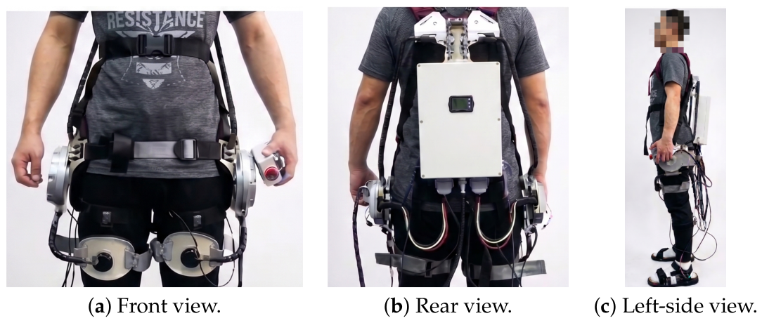
Figure 1. Active power-assist hip exoskeleton platform shown for hardware and fit documentation. The identification data were acquired in the pedestal-mounted configuration described in Section 2.1, not during human-worn gait. The panels were cropped from the original composite image to replace embedded Chinese labels with English subcaptions.
Actuators 15 00447 g001
Figure 2. Single-link equivalent model of the hip exoskeleton system. Here, q 1 is the hip angle, m t is the thigh mass, I t is the thigh moment of inertia, L t is the segment length, h G t is the distance from the center of mass to the link axis, and L G t is the projection of the center-of-mass position in the adopted frame. The original Chinese legend has been excluded by clipping and is reproduced here in English.
Actuators 15 00447 g002
Figure 3. Revised result presentation without an obstructive inset: (a) measured validation torque and representative reconstructions; (b) signed validation residuals; (c) validation RMSE distributions over 30 runs, with the deterministic BCLS value shown by the dashed line; and (d) median training convergence with IQR bands. Legends are placed outside the data regions.
Actuators 15 00447 g003
Figure 4. Sensitivity analysis: (a) median and IQR of RLS–AGWO validation RMSE over 10 seeds at five RLS-bound expansion margins; and (b) BCLS validation RMSE at five low-pass cutoff frequencies.
Actuators 15 00447 g004
Table 1. Compact pseudocode of the proposed RLS–AGWO procedure.
StepOperation
Inputs: stacked regressor H , measured torque T m , population size N, and maximum iteration count G.
Output: best base-parameter vector X * .
1Initialize λ = 0.98 , P ( 0 ) = 10 4 I , and X ^ ( 0 ) = 0 .
2For k = 1 , , K , update K ( k ) , X ^ ( k ) , and P ( k ) using Equations (7)–(9).
3Discard the first 1.0 s, obtain the componentwise extrema of the retained X ^ ( k ) , and expand them by 10% to form [ L , U ] .
4Compute γ and μ ( γ ) using Equations (10) and (12).
5Draw N initial wolves uniformly from [ L , U ] .
6For g = 1 , , G , evaluate J ( X i ) and select X α , X β , and X δ .
7Update a ( g , γ ) using Equation (11).
8Update every wolf using the three GWO leaders and project the result componentwise onto [ L , U ] .
9Return X * = X α after the final iteration.
Table 2. Experimental, signal-processing, and optimizer settings.
ItemSetting
Mechanical configurationPedestal-mounted APHE; fixed trunk; locked knee and ankle; sagittal-plane hip motion
Hip actuation and sensingBrushless DC motor; 156:1 planetary gearhead; output-shaft torque measurement
Calibration/validation motionEquations (18) and (19); durations 5 and 7 s
Sampling and retained samples100 Hz; 500/700 raw and 460/660 retained calibration/validation samples
Signal processingFourth-order 15 Hz zero-phase Butterworth filter; central finite-difference velocity and acceleration; 0.2 s endpoint exclusion
RLS initialization λ = 0.98 , P ( 0 ) = 10 4 I , X ^ ( 0 ) = 0
Search boundsRLS trajectory after 1.0 s burn-in; componentwise range enlarged by 10%
Common stochastic budget N = 30 , G = 80 , 2400 evaluations/run, 30 independent seeds; fixed-budget stop
PSO settingsInertia 0.9 0.4 ; cognitive/social coefficients c 1 = c 2 = 2.0
GA settingsTournament size 3; crossover 0.9; mutation 0.2 per gene; Gaussian scale 0.05 of span; elitism 2
GWO/AGWO settingsStandard GWO linear schedule; AGWO μ base = 0.45 , κ = 0.25 , and γ = 0.0328
Fitness and constraintsTorque RMSE in Equation (13); componentwise boundary projection
Computing environmentIntel Core i5-14600KF, 32 GB RAM, Windows 11 Pro
Table 3. Calibration and independent-validation results. Stochastic entries summarize 30 runs.
MethodTrain MeanValidation Mean ± SDValidation MedianIQRTime (ms)
LS0.14190.11520.11520.13
BCLS0.14190.11520.11520.13
Standard PSO0.6660 0.5772 ± 0.8021 0.18880.1214–0.4808 3.37 ± 0.58
RLS–PSO0.1420 0.1153 ± 0.0004 0.11520.1152–0.1153 3.35 ± 0.64
RLS–GA0.1419 0.1152 ± 0.0001 0.11520.1152–0.1153 43.31 ± 2.10
RLS–GWO0.1672 0.1552 ± 0.0171 0.15620.1439–0.1701 5.08 ± 2.19
RLS–AGWO0.1659 0.1505 ± 0.0196 0.15160.1317–0.1657 4.78 ± 1.00
Table 4. Base-parameter estimates.
Method M xt M yt J t f c f v
Reference1.5000 0.2000 1.10000.80002.5000
BCLS1.4994 0.2015 1.09950.74662.5269
RLS–PSO median1.4994 0.2016 1.09950.74632.5268
RLS–GA median1.4993 0.2013 1.09940.74642.5270
RLS–GWO median1.4977 0.2007 1.10140.73722.5354
RLS–AGWO median1.5054 0.2152 1.10370.74192.5316
Disclaimer/Publisher’s Note: The statements, opinions and data contained in all publications are solely those of the individual author(s) and contributor(s) and not of MDPI and/or the editor(s). MDPI and/or the editor(s) disclaim responsibility for any injury to people or property resulting from any ideas, methods, instructions or products referred to in the content.