Safety-Constrained Robust Backstepping Control with Dual-MRD Force Allocation for Double-Rope Mine Hoist

Abstract

Payload eccentricity and time-varying rope length can cause excessive inter-rope tension imbalance in a double-rope mine hoist. This study develops a safety-constrained semi-active differential-tension control method using dual magnetorheological dampers (MRDs). A coupled longitudinal model with time-varying rope length separates eccentricity-induced static load sharing from vibration-induced dynamic tension. A barrier Lyapunov function (BLF)-based robust backstepping controller regulates the dynamic tension-imbalance deviation about the shifted equilibrium and incorporates the prescribed 10% tension-imbalance limit into the control design. To ensure actuator feasibility, the nominal differential-force command is processed through a physically constrained MRD realization layer involving force projection, force allocation, and current regulation. Numerical results under nominal conditions show that the proposed strategy reduces the maximum tension-imbalance ratio from 0.1380 to 0.0404, produces no numerical boundary violation, and decreases the peak inter-rope tension difference during deceleration from 19.51 to 1.89 kN. Sensitivity analyses further demonstrate that the proposed controller maintains positive safety margins across all investigated variations in payload eccentricity, payload mass, hoisting acceleration, maximum hoisting speed, and maximum allowable MRD current.

1. Introduction

As mining depth, payload, and hoisting speed increase, mine hoists are moving toward longer, heavier, and faster operation. Hoisting ropes are subjected to static loads from the conveyance, payload, and self-weight, as well as dynamic excitation from rope-length variation, acceleration, deceleration, and load eccentricity, resulting in longitudinal vibration and tension fluctuations [1,2]. In double-rope systems, eccentric loading, rope-length and stiffness mismatches, and asymmetric disturbances may cause uneven load sharing and excessive tension in one rope [3,4]. Safe operation therefore requires both vibration suppression and real-time regulation of inter-rope tension imbalance to reduce local overloading, fatigue damage, and rope-failure risk.

The hoisting rope is a distributed flexible component with a time-varying length. Its longitudinal response is governed not only by the terminal payload but also by drum–rope interaction, head-sheave transmission, guide disturbances, structural flexibility, and drivetrain excitation. Hu et al. [5] developed a coupled dynamic model of the transmission and hoisting subsystems of a double-rope winding hoist and experimentally showed that gearbox cracks can be identified from the single-rope tension and inter-rope tension-difference responses. Xu et al. [6] combined flexible multibody dynamics with finite-element analysis to evaluate the dynamic stresses in the drum and main shaft of a friction hoist under time-varying loads. Pi et al. [7] established a three-dimensional model of a multi-cable winding hoist by considering the bidirectional coupling among the conveyance, flexible guides, and hoisting ropes, thereby revealing the effects of spatial eccentricity and out-of-plane excitation. Zhang et al. [8] proposed an improved Lucas–Kanade vision method to measure the lateral and longitudinal displacements of moving hoisting ropes. Zhu et al. [9] developed and experimentally validated an ADAMS-based virtual prototype to investigate longitudinal rope responses under periodic drum excitation and guide-induced impacts. These studies show that deep-mine hoisting-rope tension is governed by coupled, time-varying disturbances, while excessive fluctuations increase the risks of impact, fatigue, overloading, slippage, and rope failure. Compared with single-rope systems, double-rope winding hoists face a safety-critical load-sharing challenge. Payload eccentricity, rope-length and stiffness mismatches, installation errors, and asymmetric disturbances can cause unequal static and dynamic tensions, even between nominally identical ropes. Chinese coal mine safety regulations [10] therefore require the deviation in each rope tension from the mean tension to remain within 10%. Li et al. [11] developed and experimentally validated a signal-delay compensator and nonlinear adaptive fuzzy controller for double-rope tension coordination under communication delays, uncertainties, and disturbances. Chen et al. [12] proposed a fault-tolerant dynamic-surface controller incorporating neural-network-based fault estimation, fuzzy actuator allocation, and state constraints. Wang and Cao [13] combined an exact head-rope–tail-rope model with disturbance-observer-based adaptive neural boundary control to suppress loading-induced tension fluctuations. Deng et al. [14] applied MRDs with fuzzy skyhook control to reduce conveyance vibration, while Shi et al. [15] used optical projection and machine vision to detect abnormal rope arrangement in ultra-deep hoists. Although these studies have advanced tension coordination, vibration control, and safety monitoring, most rely on active actuators and address individual dynamic issues separately. Moreover, tension imbalance is typically treated as a performance index rather than a hard safety constraint. Therefore, this study aims not only to reduce the tension difference but also to keep the normalized imbalance within the prescribed safety limit throughout hoisting.

MRDs offer a promising alternative to fully active tension-control devices because they provide rapidly adjustable damping with low power consumption and do not continuously inject energy into the system. In our previous study [16], a spring–MRD parallel suspension and adaptive sliding-mode control were developed for longitudinal vibration suppression in a single-rope hoist. Although effective, the method did not address load sharing in double-rope systems. Masa’id et al. [17] reviewed major MR-based control strategies and stressed matching controllers to actuator limits. Zhang et al. [18] combined an MRD with sliding-mode control for broadband vibration suppression. Yoon et al. [19] showed that finite current-response time affects semi-active performance. Xu et al. [20] experimentally validated an invertible MRD force-tracking model for stay cables. Wang et al. [21] developed a dual-coil torsional MR damper with skyhook control, while Viadero-Monasterio et al. [22] proposed a current-dependent hysteresis model and robust output-feedback controller using measurable suspension deflection. However, existing MRD studies mainly address single-structure vibration or individual force tracking. In double-rope systems, the desired differential force may be infeasible because of force, current, driver, hysteresis, and modeling constraints. Practical dual-MRD control therefore requires force-feasibility analysis, constrained allocation, and compensation for implementation errors.

BLFs provide a systematic way to embed the 10% tension-imbalance limit into the controller. Unlike conventional PID, sliding-mode, and disturbance-rejection controllers, which typically verify constraints only after simulation, a BLF enforces them during control design: it approaches infinity near the prescribed boundary, and its boundedness guarantees forward invariance of the safe set. Tee and Ge [23] established an early BLF framework for nonlinear systems with partial state constraints. Wei et al. [24] combined an asymmetric time-varying integral BLF with actor–critic learning and optimized backstepping for dynamic full-state constraints. McIlvanna et al. [25] developed a BLF-based adaptive fixed-time controller for uncertain surface vessels with output constraints. Jastrzębski and Kabziński [26] investigated practical BLF tuning under actuator saturation, measurement errors, and noise. Hong et al. [27] integrated a logarithmic BLF with finite-time backstepping, neural approximation, and auxiliary dynamics for simultaneous state and input constraints. Niu et al. [28] proposed adaptive BLF control for pure-feedback systems with full-state constraints and asymptotic tracking. Hosseinnajad et al. [29] and Li et al. [30] applied BLF-based control to constrained vehicle path tracking and shuttle transport, respectively. Cheng et al. [31] addressed full-state constraints in nonlinear power systems, while Song et al. [32] used a symmetric BLF for a flexible manipulator with input and state constraints. These studies show that BLFs can integrate stability and safety constraints. However, existing work has not simultaneously addressed normalized tension imbalance in variable-length double-rope hoists, state-dependent dual-MRD force limits, constrained differential-force allocation, driver dynamics, and force-realization errors. Therefore, this study imposes the 10% imbalance limit as a hard output constraint, incorporates the force-realization error into the matched uncertainty in the strict analysis, and evaluates the effect of feasibility projection numerically. More broadly, nonlinear structural dynamics and vibration regulation have also been investigated in flexible systems outside mine hoisting applications. Zhao et al. [33] analyzed the nonlinear aeroelastic response and flutter control of bistable composite laminated cantilever plates, highlighting the influence of structural nonlinearity and operating conditions on dynamic stability. Liu et al. [34] developed a quasi-zero-stiffness device using piezoelectric buckled beams and demonstrated its effectiveness for low frequency vibration isolation and energy harvesting. Although these systems differ physically from mine hoisting ropes, they provide useful methodological references for nonlinear vibration modeling and response regulation under varying operating conditions. In the present study, these considerations are extended to safety-constrained tension balancing in a variable-length double-rope hoisting system with semi-active MRD actuation.

Accordingly, this study develops a safety-constrained semi-active differential-tension balancing framework for a double-rope mine hoist equipped with dual-MRDs. The main contributions are summarized as follows:

(1)

A unified variable-length double-rope model is established by separating eccentricity-induced static load sharing from vibration-induced dynamic tension. A signed normalized tension-imbalance ratio is constructed from the reconstructed total rope tensions.

(2)

A BLF-based robust backstepping controller is developed to generate the nominal differential-force demand. The prescribed 10% tension-imbalance boundary is embedded in the control design, and bounded matched uncertainties are compensated using a continuous robust term. Under an explicit control authority condition, closed-loop boundedness and forward invariance of the prescribed safe set are established on any interval during which the nominal differential force remains inside the instantaneous attainable set.

(3)

A physically constrained actuator realization layer is developed to convert the nominal differential-force command into feasible dual-MRD force and current commands while considering actuator limitations and realization errors.

The remainder of this paper is organized as follows. Section 2 establishes the eccentric-load and variable-length dynamic model of the double-rope hoisting system. Section 3 presents the state-dependent MRD force limits, bounded inverse mapping, current-driver dynamics, and constrained force-allocation method. Section 4 develops the BLF-based robust backstepping controller and presents the stability and constraint-satisfaction analysis. Section 5 reports the numerical results and engineering discussion, and Section 6 presents the conclusions.

2. Dynamic Model of the Double-Rope Hoisting System

2.1. Physical Configuration of the Double-Rope System

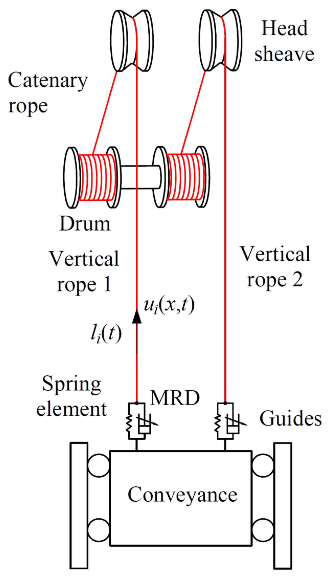
As shown in Figure 1, the double-rope mine hoisting system comprises two parallel hoisting ropes wound on two drum sections mounted on a common shaft. Each rope extends from the drum through a catenary segment, passes over an individual head sheave, and continues vertically to the conveyance. For the i-th rope (i = 1,2), the time-varying length of the vertical rope segment is denoted by l_i(t), and its longitudinal displacement is represented by u_i(x, t), where x ∈ [0, l_i(t)] is the spatial coordinate measured downward from the head-sheave tangent point. Thus, x = 0 and x = l_i(t) correspond to the upper and lower ends of the vertical rope segment, respectively.

Before each hoisting cycle, adjustable preload mechanisms compensate for initial rope-length mismatches and installation deviations and establish the prescribed static suspension state. The preload settings are subsequently locked and incorporated into the calibrated static rope tensions. Each lower suspension unit consists of a load-bearing spring and an MRD connected in parallel, with the MRD supplying an adjustable dissipative force to suppress dynamic rope-tension fluctuations. The dynamics of the catenary ropes, drums, and head sheaves are not modeled explicitly; their effects on the vertical rope segments are represented by equivalent upper-boundary disturbances. The guide system is assumed to constrain the lateral and rotational motions of the conveyance without transmitting significant static vertical force or overturning moment. Residual guide interactions, rotational coupling, and unmodeled transmission effects are included in the disturbance terms.

2.2. Eccentricity-Induced Static Load Sharing and Total Tension Imbalance

In practical hoisting operations, the center of gravity of the conveyance–payload assembly may deviate from the midpoint of the two suspension points because of asymmetric structural mass, uneven payload distribution, off-center loading, or payload migration. The static load-sharing analysis assumes that the guide system does not transmit a significant vertical reaction or static overturning moment. Its residual dynamic influence is incorporated into the disturbance model.

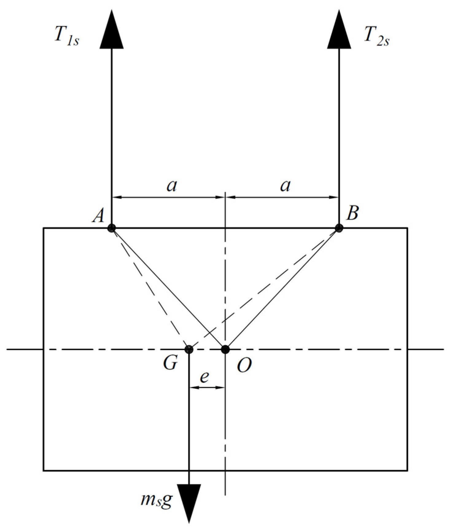
As shown in Figure 2, A and B denote the two suspension points, O is their midpoint, and the distance between the suspension points is 2a. The total mass of the conveyance–payload assembly is m_s, and its center of gravity is denoted by G. The signed horizontal eccentricity e is defined as positive when G shifts from O toward suspension point A.

Under static equilibrium, the vertical force balance and moment balance about O are given by

$$T_{1s}+T_{2s}=m_{s}g,$$

(1)

$$a\left(T_{1s}-T_{2s}\right)=m_{s}ge,$$

(2)

where T_1s and T_2s are the static tensions of the two ropes. Solving Equations (1) and (2), the static tensions of the two ropes are obtained as

$$\left\{\begin{array}{l}{T}_{1s}={\displaystyle \frac{m_{s}g}{2}}\left(1+{\displaystyle \frac{e}{a}}\right)\\ T_{2s}={\displaystyle \frac{m_{s}g}{2}}\left(1-{\displaystyle \frac{e}{a}}\right)\end{array}\right..$$

(3)

Condition |e| < a guarantees positive static tension in both ropes. The corresponding signed static tension-imbalance ratio is defined as

$${\eta }_s={\displaystyle \frac{T_{1s}-T_{2s}}{T_{1s}+T_{2s}}}={\displaystyle \frac{e}{a}}.$$

(4)

A positive residual dynamic safety margin additionally requires

$$\left|{\eta }_s\right|={\displaystyle \frac{\left|e\right|}{a}}<{\eta }_{\max },$$

which is more restrictive than the positive-tension condition when η_max < 1.

The total tension of the i-th rope is decomposed into its calibrated static component and dynamic perturbation as

$$T_i\left(t\right)=T_{is}+T_{id}\left(t\right),\hspace{1em}i=1,2,$$

(5)

where T_id(t) is the signed dynamic tension perturbation caused by rope vibration, hoisting acceleration, upper-boundary excitation, suspension motion, MRD action, and external disturbances.

The mean rope tension, total inter-rope tension difference, and dynamic inter-rope tension difference are defined as

$$\left\{\begin{array}{l}\overline{T}\left(t\right)={\displaystyle \frac{T_1\left(t\right)+T_2\left(t\right)}{2}}\\ \Delta T\left(t\right)=T_1\left(t\right)-T_2\left(t\right)\\ \Delta T_d\left(t\right)=T_{1d}\left(t\right)-T_{2d}\left(t\right)\end{array}\right..$$

(6)

The signed normalized total tension-imbalance ratio is defined as

$$\eta \left(t\right)={\displaystyle \frac{T_1\left(t\right)-T_2\left(t\right)}{T_1\left(t\right)+T_2\left(t\right)}}={\displaystyle \frac{\Delta T\left(t\right)}{2\overline{T}\left(t\right)}},$$

(7)

where T₁(t) + T₂(t) > 0 during normal hoisting operation.

The dynamic deviation from the calibrated static equilibrium is defined as

$$\tilde{\eta }(t)=\eta (t)-{\eta }_s.$$

(8)

According to the Coal Mine Safety Regulations of China [10], the deviation in the tension in each rope from the mean rope tension should not exceed 10%. For the present two rope system, the normalized deviation in either rope from the mean tension is equivalent to the absolute value of the tension-imbalance ratio defined in Equation (7). Therefore, the prescribed total tension-imbalance safety requirement is

$$\left|\eta \left(t\right)\right|\le {\eta }_{\max }, {\eta }_{\max }=0.1.$$

(9)

Because the preload mechanisms remain locked during hoisting, the calibrated static imbalance η_s is not an online control variable. Therefore, the controller regulates the dynamic deviation defined in Equation (8) about the eccentricity-dependent static equilibrium.

The residual dynamic safety margin is defined as

$$k_b={\eta }_{\max }-\left|{\eta }_s\right|>0.$$

(10)

If $\left|\tilde{\eta }\left(t\right)\right|<k_b$, then

$$\left|\eta \left(t\right)\right|\le \left|{\eta }_s\right|+\left|\tilde{\eta }\left(t\right)\right|<{\eta }_{\max }.$$

(11)

Therefore, constraining the dynamic deviation within the residual margin is sufficient to maintain the total tension-imbalance ratio inside the prescribed safety region.

2.3. Coupled Variable-Length Longitudinal Dynamics

The hoisting-rope system consists of catenary-rope segments, vertical variable-length rope segments, and the lower suspension units. Because the differential-tension balancing problem considered in this study is primarily associated with the conveyance side, the two vertical rope segments are selected as the distributed-parameter controlled objects. The effects of drum vibration, catenary-rope dynamics, and head-sheave transmission are represented by equivalent upper-boundary disturbances.

The longitudinal dynamics of the i-th variable-length rope are written as

$$\rho \left[{\displaystyle \frac{{\partial }^2{u}_i}{\partial t^2}}+2V(t){\displaystyle \frac{{\partial }^2{u}_i}{\partial x\partial t}}+\dot{V}(t){\displaystyle \frac{\partial u_i}{\partial x}}+V^2(t){\displaystyle \frac{{\partial }^2{u}_i}{\partial x^2}}+\dot{V}(t)\right]-EA{\displaystyle \frac{{\partial }^2{u}_i}{\partial x^2}}=0,$$

(12)

where ρ is the rope mass per unit length, EA is the axial stiffness, and V(t) is the hoisting velocity, and $\dot{V}(t)=dV(t)/dt$ is the hoisting acceleration.

The effects of the fixed length catenary rope and head-sheave subsystem are represented through an equivalent upper-boundary displacement obtained from a reduced longitudinal model of the catenary rope. For the i-th rope, the longitudinal displacement of the fixed length catenary segment is denoted by $u_{c,i}(x_c,t),x_c\in [0,l_c]$ and is governed by the moving rope longitudinal equation

$$\rho \left[{\displaystyle \frac{{\partial }^2{u}_{c,i}}{\partial t^2}}+2V(t){\displaystyle \frac{{\partial }^2{u}_{c,i}}{\partial x\partial t}}+\dot{V}(t){\displaystyle \frac{\partial u_{c,i}}{\partial x}}+V^2(t){\displaystyle \frac{{\partial }^2{u}_{c,i}}{\partial x^2}}+\dot{V}(t)\right]-EA{\displaystyle \frac{{\partial }^2{u}_{c,i}}{\partial x^2}}=0,$$

(13)

The drum side is fixed in the perturbation coordinate, u_c,i(0, t) = 0. Its displacement at the head-sheave side,

$$d_i\left(t\right)=u_{c,i}\left(l_c,t\right),$$

is used as the upper-boundary excitation of the corresponding variable-length vertical rope,

$$u_i\left(0,t\right)=d_i\left(t\right),$$

where d_i(t) denotes the equivalent longitudinal disturbance transmitted to the upper end of the i-th vertical rope.

The relative deformation and relative velocity of the i-th spring–MRD suspension unit are defined as

$$x_{mi}\left(t\right)=y\left(t\right)-u_i\left(l_i\left(t\right),t\right),$$

(14)

$${\dot{x}}_{mi}\left(t\right)=\dot{y}\left(t\right)-{\dot{u}}_i\left(l_i\left(t\right),t\right)-{\dot{l}}_i\left(t\right){u^{\prime }}_i\left(l_i\left(t\right),t\right).$$

(15)

The spring force is defined as

$$F_{pi}\left(t\right)=k_{pi}{x}_{mi}\left(t\right),$$

(16)

where k_pi > 0 is the stiffness of the i-th load-bearing spring. The total dynamic force transmitted by the corresponding spring–MRD suspension unit is

$$S_i\left(t\right)=F_{pi}\left(t\right)+F_{mi}\left(t\right),$$

where F_mi(t) is the MRD force.

The lower-end force equilibrium is then written as

$$EA{u}_i^{\prime }\left(l_i\left(t\right),t\right)=S_i\left(t\right)+d_{bi}\left(t\right),$$

(17)

where d_bi(t) represents the lower-boundary force disturbance.

The vertical perturbation dynamics of the conveyance can be written as

$$m_s\ddot{y}\left(t\right)+S_1\left(t\right)+S_2\left(t\right)=d_y\left(t\right),$$

(18)

where d_y(t) includes residual guide interaction, small rotational coupling, and external vertical disturbances.

The initial displacement and velocity fields, together with the initial conveyance states, are specified consistently with the calibrated stationary condition in the numerical simulations.

2.4. Galerkin Discretization and Tension Reconstruction

To transform the moving spatial domain into a fixed domain, introduce

$$\xi ={\displaystyle \frac{x}{l(t)}},\hspace{1em}\xi \in [0,1].$$

(19)

The displacement field is approximated by a lifting function satisfying the nonhomogeneous upper-boundary condition and a finite modal expansion as

$$u_i(x,t)=(1-\xi )d_i(t)+{\displaystyle \sum _{r=1}^N{\varphi }_r}(\xi )q_{ir}(t),$$

(20)

where q_ir(t) is the r-th generalized coordinate of the i-th rope. The admissible functions satisfy the essential upper-boundary condition ϕ_r (0) = 0. In the present implementation, ϕ_r(ξ) = sin[(r − 1/2)πξ]. The lower-end force condition in Equation (17) is introduced as a natural boundary condition in the Galerkin weak formulation.

Define the modal-coordinate vector of the i-th rope and the augmented generalized-coordinate vector as

$$q_i\left(t\right)={\left[\begin{array}{c}{q}_{i1}\left(t\right)\cdots q_{iN}\left(t\right)\end{array}\right]}^T,\hspace{1em}\chi \left(t\right)={\left[\begin{array}{c}{q}_1^T\left(t\right)\hspace{1em}{q}_2^T\left(t\right)\hspace{1em}y\left(t\right)\end{array}\right]}^T.$$

Substituting Equation (20) into Equation (12), applying the boundary and conveyance relations in Equations (13)–(18), and performing the Galerkin projection yield the coupled finite-dimensional model of the double-rope–conveyance system, which can be written as

$$M(t)\ddot{\chi }+C(t)\dot{\chi }+K(t)\chi =q_0\left(t\right)+B_m\left(t\right)F_m(t)+B_d\left(t\right)d(t),$$

(21)

where

$$F_m={\left[F_{m1},F_{m2}\right]}^T.$$

Here, M(t) is the generalized mass matrix; C(t) contains the convective, gyroscopic, and rope-length-variation terms; K(t) contains the rope axial-stiffness and suspension-spring contributions; q₀(t) collects the known terms generated by the lifting functions and prescribed hoisting motion; and B_m(t) and B_d(t) are the actuator and disturbance distribution matrices, respectively.

Because the lower-end traction is introduced through the natural boundary condition, the total tension at the lower end of the i-th rope is reconstructed from the boundary equilibrium as

$$T_i(t)=T_{is}+S_i(t)+d_{bi}(t).$$

(22)

3. Dual-MRD Force Feasibility and Realization

The upper-level BLF controller determines the differential-force demand required for tension-imbalance regulation. However, this ideal control command cannot be directly applied to the hoisting system because the MRDs are subject to state-dependent force limits, bounded current amplitudes, nonlinear force–current characteristics, and finite current-driver dynamics. Therefore, this section establishes the actuator realization layer, including attainable force evaluation, constrained dual-MRD allocation, inverse current mapping, and force-realization error modeling.

3.1. MRD Actuator Interface

The MRD forward model and force-to-current inverse mapping are adopted from the validated actuator model developed in our previous work [16]. Since the present study focuses on system-level tension balancing rather than MRD constitutive modeling, only the compact actuator interface required for controller implementation is introduced here.

For the i-th MRD, the actuator interface is written compactly as:

$$F_{mi}\left(t\right)=f_{\mathrm{MRD}}\left(x_{mi}\left(t\right),{\dot{x}}_{mi}\left(t\right),I_i\left(t\right)\right),\hspace{1em}i=1,2,$$

(23)

where I_i(t) ∈ [0, I_max] is the applied coil current.

For an attainable target force $F_{mi}^{\ast }$ the bounded inverse solution is defined as

$$J_i(t)=\left\{I\in \left[0,I_{\max }\right]:f_{\mathrm{MRD}}\left(x_{mi}\left(t\right),{\dot{x}}_{mi}\left(t\right),I\right)=F_{mi}^{\ast }\left(t\right)\right\}.$$

(24)

When multiple inverse solutions exist, the current command is selected as

$$I_i^c\left(t\right)=\underset{I\in J_i^{\ast }\left(t\right)}{\mathrm{argmin}}\left|I-I_i^c\left(t^{-}\right)\right|,$$

(25)

where $I_i^c(t^{-})$ denotes the current command at the preceding sampling instant. This selection avoids unnecessary switching between inverse branches and improves the continuity of the current command. When the force–current relationship is monotonic over the instantaneous operating state, Equation (25) reduces to the unique bounded inverse solution established in Ref. [16].

3.2. State-Dependent Attainable Force Range

Because an MR damper is a semi-active actuator, its attainable force range depends on the instantaneous relative deformation, relative velocity, and admissible current interval. Therefore, the force limits are evaluated online rather than represented by constant saturation bounds.

For the i-th MRD, the raw force set over the admissible current interval is

$${\mathcal{F}}_{i,\mathrm{raw}}(t)=\{f_{\mathrm{MRD}}\left(x_{mi}(t),{\dot{x}}_{mi}(t),I\right):0\le I\le I_{\max }\}.$$

(26)

With the force convention adopted in this study, the semi-active dissipativity condition is written as

$$F{\dot{x}}_{mi}\le {\epsilon }_P,$$

where ε_P ≥ 0 is a small power tolerance introduced to avoid numerical rejection near zero relative velocity. The instantaneous attainable force set is therefore

$${\mathcal{F}}_i(t)=\left\{F\in {\mathcal{F}}_{i,\mathrm{raw}}(t):F{\dot{x}}_{mi}\le {\epsilon }_P\right\}.$$

(27)

Because the MRD force is continuous with respect to the current over the compact interval [0, I_max], the attainable force bounds exist and are defined as

$$F_{i,\min }(t)={\min }_{F\in {\mathcal{F}}_i(t)}F,\hspace{1em}{F}_{i,\max }(t)={\max }_{F\in {\mathcal{F}}_i(t)}F.$$

(28)

Hence,

$${\mathcal{F}}_i(t)=\left[F_{i,\min }(t),F_{i,\max }(t)\right].$$

Defining the differential MRD force as

$$F_d(t)=F_{m1}(t)-F_{m2}(t).$$

The instantaneous attainable differential-force interval generated by the two MRDs is

$$\mathcal{D}(t)=\left[{\mathcal{D}}_{\min }(t),{\mathcal{D}}_{\max }(t)\right],$$

(29)

where

$${\mathcal{D}}_{\min }(t)=F_{1,\min }(t)-F_{2,\max }(t),\hspace{1em}{\mathcal{D}}_{\max }(t)=F_{1,\max }(t)-F_{2,\min }(t)$$

Equations (26)–(29) characterize the instantaneous force capability under the current-amplitude and semi-active constraints. Transient limitations associated with the current driver are treated separately through the force-realization error introduced in Section 3.4.

3.3. Constrained Dual-MRD Force Allocation

The BLF controller generates the nominal differential-force command $F_{d,\mathrm{nom}}\left(t\right)$. If this command lies outside the instantaneous attainable interval $\mathcal{D}\left(t\right)$, it is projected onto the nearest attainable boundary as

$$\begin{array}{ll}{F}_{d,a}^{*}(t)& ={\mathrm{proj}}_{\mathcal{D}(t)}\left(F_{d,\mathrm{nom}}(t)\right)\\ & =\min \left\{\max \left[F_{d,\mathrm{nom}}(t),D_{\min }(t)\right],D_{\max }(t)\right\}\end{array}.$$

(30)

The corresponding feasibility projection error is defined as $e_{F_a}(t)=F_{d,a}^{*}(t)-F_{d,\mathrm{nom}}(t)$. Thus, $e_{F_a}(t)=0$ whenever the nominal command is directly attainable.

The individual target forces are determined as

$$\begin{array}{c}\left(F_{m1}^{*},F_{m2}^{*}\right)=\underset{F_1,F_2}{\arg \min }\hspace{1em}{w}_c{(F_1+F_2)}^2+w_u\left(F_1^2+F_2^2\right)\\ \mathrm{s}.\mathrm{t}.\hspace{1em}\hspace{1em}{F}_1-F_2=F_{d,a}^{*}\\ \hspace{1em}\hspace{1em}\hspace{1em}\hspace{1em}\hspace{1em}\hspace{1em}{F}_i\in {\mathcal{F}}_i(t),\hspace{1em}i=1,2\end{array},$$

(31)

where w_c > 0 and w_u > 0 are weighting coefficients.

The first objective term suppresses unnecessary common-mode force, which contributes little to differential-tension regulation, whereas the second term limits the overall actuator demand. Since w_u > 0, the quadratic objective is strictly convex. Moreover, because $F_{d,a}^{*}(t)\in \mathcal{D}(t)$, the feasible set is nonempty. Therefore, the allocation problem admits a unique solution. Since only two scalar actuator forces are involved, the resulting low-dimensional convex program can be solved efficiently at each sampling instant.

3.4. Current-Driver Dynamics and Force-Realization Error

Even when the allocated target force is instantaneously attainable, the actual MRD force cannot follow the target without delay because of the finite bandwidth and slew-rate limitation of the current driver. The bounded inverse-model command is therefore applied through a rate-limited first-order current driver as

$${\dot{I}}_i(t)={\mathrm{sat}}_{[-r_{i,\max },r_{i,\max }]}\left[{\displaystyle \frac{{\mathrm{sat}}_{[0,I_{\max }]}\left(I_{c,i}^{*}\left(t\right)\right)-I_i\left(t\right)}{{\tau }_i}}\right],$$

(32)

where τ_i > 0 is the current-driver time constant and r_i,max > 0 is the maximum current slew rate. For any initial current I_i(0) ∈ [0, I_max], Equation (32) ensures that I_i(t) ∈ [0, I_max].

The actual MRD force is evaluated from the applied current using Equation (23). The individual force-realization error is defined as

$$e_{Fi}(t)=F_{mi}(t)-F_{mi}^{*}(t),\hspace{1em}i=1,2.$$

(33)

The target and actual differential forces satisfy

$$\left\{\begin{array}{l}{F}_d^{*}\left(t\right)=F_{m1}^{*}\left(t\right)-F_{m2}^{*}\left(t\right)=F_{d,a}^{*}\left(t\right)\\ F_d\left(t\right)=F_{m1}\left(t\right)-F_{m2}\left(t\right)=F_d^{*}\left(t\right)+e_{Fr}\left(t\right)\end{array}\right.,$$

(34)

where $e_{Fr}\left(t\right)=e_{F1}\left(t\right)-e_{F2}\left(t\right)$ is the differential-force-realization error.

Over the prescribed compact MRD operating domain, the realization error is assumed to satisfy

$$|e_{Fr}(t)|\le {\overline{e}}_{Fr},$$

(35)

where ${\overline{e}}_{Fr}$ is the conservative bound, which is obtained offline from the validated MRD model, the selected current-driver parameters, and the prescribed ranges of relative displacement, relative velocity, and coil current.

4. BLF-Based Robust Backstepping Differential-Tension Controller

Using the shifted output defined in Equation (8), the controller regulates the dynamic tension-imbalance deviation $\tilde{\eta }\left(t\right)$ within the residual safety margin k_b. The resulting nominal differential-force command is subsequently processed by the actuator realization layer developed in Section 3.

4.1. Control-Oriented Differential-Tension Model

Define the finite-dimensional state vector as

$$X={\left[\begin{array}{cc}{\chi }^T& {\dot{\chi }}^T\end{array}\right]}^T.$$

(36)

The coupled finite-dimensional model in Equation (21) can be written in the control-affine form as

$$\dot{X}=f_x(X,t)+G_m(X,t)F_m\left(t\right)+G_d(X,t)d\left(t\right),$$

(37)

where

$$f_x(X,t)=\left[\begin{array}{c}\dot{\chi }\\ M^{-1}\left(t\right)\left(q_0\left(t\right)-C\left(t\right)\dot{\chi }-K\left(t\right)\chi \right)\end{array}\right],$$

$$\begin{gathered} G_m(X,t)=\left[\begin{array}{c}0\\ M^{-1}(t)B_m(t)\end{array}\right], \\ {G}_d(X,t)=\left[\begin{array}{c}0\\ M^{-1}(t)B_d(t)\end{array}\right]. \end{gathered}$$

The normalized total tension imbalance reconstructed from Equation (22) is represented by the nonlinear output

$$\eta \left(t\right)=h(X,t),\hspace{1em}\tilde{\eta }\left(t\right)=h\left(X,t\right)-{\eta }_s.$$

(38)

Relative Degree and Differential-Force Effectiveness

To demonstrate the input–output structure used in the controller design, the lower-end tension vector reconstructed from the finite-dimensional coordinates is written as

$$T(\chi ,t)=\left[\begin{array}{c}{T}_1(\chi ,t)\\ T_2(\chi ,t)\end{array}\right].$$

(39)

Define

$$a_{\Delta }=\left[\begin{array}{c}1\\ -1\end{array}\right],\hspace{1em}{a}_{\Sigma }=\left[\begin{array}{c}1\\ 1\end{array}\right].$$

(40)

The inter-rope tension difference and total tension are

$$\Delta T=a_{\Delta }^{T}T,\hspace{1em}\Sigma T=a_{\Sigma }^{T}T,$$

(41)

and the normalized tension-imbalance output is

$$\eta =h(\chi ,t)={\displaystyle \frac{\Delta T}{\Sigma T}}.$$

(42)

Let

$$J_T(\chi ,t)={\displaystyle \frac{\partial T}{\partial \chi }}.$$

(43)

denote the tension reconstruction Jacobian. Because the output depends on the generalized coordinates but not directly on their velocities or the differential-force input, its first derivative is

$$\dot{\tilde{\eta }}=h_{\chi }\dot{\chi }+h_t,$$

(44)

where

$$h_{\chi }={\displaystyle \frac{\Sigma T{a}_{\Delta }^T{J}_T-\Delta T{a}_{\Sigma }^T{J}_T}{{(\Sigma T)}^2}}.$$

(45)

Therefore, the differential force does not appear in the first derivative of the output.

The individual MRD forces are decomposed into common mode and differential components as

$$F_m=b_c{F}_c+b_{\Delta }{F}_d,$$

(46)

with

$$b_c={\displaystyle \frac{1}{2}}\left[\begin{array}{c}1\\ 1\end{array}\right],\hspace{1em}{b}_{\Delta }={\displaystyle \frac{1}{2}}\left[\begin{array}{c}1\\ -1\end{array}\right].$$

(47)

Substituting the finite-dimensional dynamics into the second derivative of the output gives

$$\ddot{\tilde{\eta }}=f_T(X,t)+g_T(X,t)F_d(t)+d_0(t),$$

(48)

where f_T denotes the nominal differential-tension dynamics, g_T is the differential-force effectiveness coefficient, and d₀(t) includes parameter perturbations, residual eccentric-load variation, modal-truncation error, upper-boundary uncertainty, guide interaction, and other bounded disturbances.

The differential-force effectiveness coefficient is

$$g_T(X,t)=h_{\chi }(\chi ,t)M^{-1}(t)B_m(t)b_{\Delta }.$$

(49)

Equivalently,

$$g_T(X,t)={\displaystyle \frac{[\Sigma T{a}_{\Delta }^T{J}_T-\Delta T{a}_{\Sigma }^T{J}_T]M^{-1}{B}_m{b}_{\Delta }}{{(\Sigma T)}^2}}.$$

(50)

Hence, the differential-force input is absent from $\dot{\tilde{\eta }}$ and appears explicitly in $\ddot{\tilde{\eta }}$. The output therefore has relative degree two wherever

$$g_T(X,t)\ne 0.$$

(51)

Using Equations (30) and (34), the actual differential force can be expressed relative to the nominal controller output as

$$F_d(t)=F_{d,\mathrm{nom}}(t)+e_{Fa}(t)+e_{Fr}(t).$$

(52)

To distinguish the strict analytical case from the implemented projected case, define the no-projection time set as

$${\mathcal{I}}_{\mathrm{np}}=\left\{t\in [0,t_f]:F_{d,\mathrm{nom}}(t)\in \mathcal{D}(t)\right\},$$

where D(t) denotes the instantaneous attainable differential-force interval. The corresponding projection time set is

$${\mathcal{I}}_{\mathrm{p}}=[0,t_f]\backslash {\mathcal{I}}_{\mathrm{np}}.$$

For $t\in {\mathcal{I}}_{\mathrm{np}}$, the nominal differential force is directly attainable, and therefore

$$F_{d,a}^{*}(t)=F_{d,\mathrm{nom}}(t),\hspace{1em}{e}_{Fa}(t)=0.$$

The strict control-oriented dynamics then reduce to

$$\ddot{\tilde{\eta }}=f_T\left(X,t\right)+g_T\left(X,t\right)F_{d,\mathrm{nom}}\left(t\right)+{\Delta }_T\left(t\right),$$

(53)

where

$${\Delta }_T\left(X,t\right)=d_0\left(t\right)+g_T\left(X,t\right)e_{Fr}\left(t\right)$$

(54)

is the bounded matched uncertainty considered in the strict stability analysis.

For quantitative uncertainty assessment, the lumped matched uncertainty is further decomposed into modeling uncertainty, external disturbance contribution, and differential-force-realization error as

$${\Delta }_T(t)=d_{\mathrm{mod}}(t)+d_{\mathrm{ext}}(t)+g_T(X,t)e_{Fr}(t),$$

(55)

where d_mod(t) represents the equivalent output channel contribution of modeling uncertainty, including parameter perturbations, Galerkin modal truncation, residual eccentric-load variation, and other unmodeled dynamics. The term d_ext(t) represents the equivalent contribution of the prescribed upper-boundary disturbances, lower-boundary force disturbances, residual guide interaction, and external conveyance disturbances. The term e_Fr(t) denotes the differential-force-realization error caused by the finite current-driver dynamics, current slew-rate limitation, and MRD hysteresis. The feasibility projection error is not included in Equation (55), because the strict stability result is restricted to intervals without feasibility projection.

For $t\in {\mathcal{I}}_{\mathrm{p}}$, feasibility projection is activated and $e_{Fa}(t)\ne 0$. The actual output dynamics are then

$$\ddot{\tilde{\eta }}=f_T\left(X,t\right)+g_T\left(X,t\right)F_{d,\mathrm{nom}}\left(t\right)+{\Delta }_T\left(t\right)+g_T\left(X,t\right)e_{Fa}\left(t\right).$$

Because the projection-induced term $g_T{e}_{Fa}$ is not included in the uncertainty bound used in the following theorem, the strict analytical result applies only to no-projection intervals contained in ${\mathcal{I}}_{\mathrm{np}}$.

Define the control-oriented states as

$$x_1=\tilde{\eta },\hspace{1em}{x}_2=\dot{\eta }.$$

(56)

Therefore,

$$\left\{\begin{array}{l}{\dot{x}}_1=x_2\\ {\dot{x}}_2=f_T+g_T{F}_{d,\mathrm{nom}}+{\Delta }_T\end{array}\right..$$

(57)

4.2. BLF-Based Robust Backstepping Control Law

The control objective is to maintain the dynamic deviation within the residual safety margin $k_b={\eta }_{\max }-\left|{\eta }_s\right|>0$ defined in Equation (10).

The first backstepping error is selected as

$$z_1=x_1=\tilde{\eta }.$$

(58)

To prevent the dynamic deviation from exhausting the residual safety margin, the logarithmic barrier Lyapunov function is chosen as

$$V_1(z_1)={\displaystyle \frac{1}{2}}\ln \left({\displaystyle \frac{k_b^2}{k_b^2-z_1^2}}\right),\hspace{1em}|z_1|<k_b.$$

(59)

Its derivative is

$${\dot{V}}_1={\displaystyle \frac{z_1{\dot{z}}_1}{k_b^2-z_1^2}}={\displaystyle \frac{z_1{x}_2}{k_b^2-z_1^2}}.$$

(60)

The virtual control signal is designed as

$${\alpha }_1=-c_1{z}_1,\hspace{1em}{c}_1>0,$$

(61)

and the second error variable is defined as

$$z_2=x_2-{\alpha }_1.$$

(62)

Substituting x₂ = z₂ + α₁ into Equation (47) gives

$${\dot{V}}_1=-c_1{\displaystyle \frac{z_1^2}{k_b^2-z_1^2}}+{\displaystyle \frac{z_1{z}_2}{k_b^2-z_1^2}}.$$

(63)

The nominal differential-force command is designed as

$$F_{d,\mathrm{nom}}={\displaystyle \frac{1}{g_T}}\left[-f_T+{\dot{\alpha }}_1-c_2{z}_2-{\displaystyle \frac{z_1}{k_b^2-z_1^2}}-k_r\tanh \left({\displaystyle \frac{z_2}{\epsilon }}\right)\right],$$

(64)

where c₂ > 0 is the second backstepping gain, k_r > 0 is the robust gain, and ε > 0 is the boundary-layer parameter.

The barrier term increases the corrective differential-force demand as |z₁| approaches k_b. The continuous hyperbolic-tangent term attenuates the bounded matched uncertainty while avoiding the severe chattering associated with a discontinuous sign function.

4.3. Constraint Satisfaction and Closed-Loop Boundedness

To establish the constraint-satisfaction and closed-loop boundedness properties of the proposed controller, the following assumptions are introduced.

Assumption 1.

The functions f_T(X, t) and g_T(X, t) are locally Lipschitz in X and piecewise continuous in t. The total rope tension remains positive

$$T_1(t)+T_2(t)\ge T_{\Sigma ,\min }>0.$$

(65)

The differential-force effectiveness coefficient has a known constant sign  $s_g\in \{-1,1\}$  and satisfies

$$0<g_{\min }\le s_g{g}_T(X,t)\le g_{\max }.$$

(66)

Assumption 2.

Over the safety certified operating domain, the modeling uncertainty, external disturbance contribution, and differential-force-realization error satisfy

$$|d_{\mathrm{mod}}(t)|\le {\overline{d}}_{\mathrm{mod}}, |d_{\mathrm{ext}}(t)|\le {\overline{d}}_{\mathrm{ext}}, |e_{Fr}(t)|\le {\overline{e}}_{Fr}.$$

Using the verified upper bound of the differential-force effectiveness coefficient,

$$|g_T(X,t)|\le g_{\max }.$$

The lumped matched uncertainty satisfies

$$|{\Delta }_T|\le {\overline{\Delta }}_T, {\overline{\Delta }}_T:={\overline{d}}_{\mathrm{mod}}+{\overline{d}}_{\mathrm{ext}}+g_{\max }{\overline{e}}_{Fr}.$$

(67)

Assumption 3.

The preload mechanisms are calibrated before hoisting and remain locked throughout the hoisting cycle. The resulting static imbalance is constant and satisfies

$$\left|{\eta }_s\right|<{\eta }_{\max },k_b={\eta }_{\max }-\left|{\eta }_s\right|>0.$$

(68)

Let

$${\mathcal{I}}_j=[t_{a,j},t_{b,j}]\subseteq {\mathcal{I}}_{\mathrm{np}}$$

denote a connected no-projection interval over which the strict analytical result is applied. At the beginning of this interval, the dynamic tension-imbalance deviation satisfies

$$\left|\overline{\eta }(t_{a,j})\right|<k_b.$$

(69)

When t_a,j = 0, Equation (69) reduces to the original initial safety condition. For a no-projection interval following a projection interval, the condition in Equation (69) must be verified from the state at t = t_a,j, because the strict analytical result developed below does not cover the preceding projection interval.

• Control authority condition on a no-projection interval.

Let

$${\mathcal{I}}_j=[t_{a,j},t_{b,j}]\subseteq {\mathcal{I}}_{\mathrm{np}}$$

be any connected no-projection interval. Over ${\mathcal{I}}_j$, the nominal differential force satisfies

$$F_{d,\mathrm{nom}}(t)\in \mathcal{D}(t),\hspace{1em}\forall t\in {\mathcal{I}}_j.$$

(70)

Consequently,

$$F_{d,a}^{*}\left(t\right)=F_{d,\mathrm{nom}}\left(t\right),\hspace{1em}{e}_{Fa}\left(t\right)=0,\hspace{1em}\forall t\in {\mathcal{I}}_j.$$

(71)

Theorem 1.

Consider the closed-loop dynamic tension-imbalance system in Equation (57) under the control law in Equation (64). Let

$${\mathcal{I}}_j=[t_{a,j},t_{b,j}]\subseteq {\mathcal{I}}_{\mathrm{np}}$$

be a connected no-projection interval. Suppose that Assumptions 1 to 3 hold, the control authority condition is satisfied over  ${\mathcal{I}}_j$, and that the robust gain satisfies

$$k_r>{\overline{\Delta }}_T.$$

(72)

Then the closed-loop errors z₁ and z₂ remain bounded over  ${\mathcal{I}}_j$, and

$$\left|\tilde{\eta }(t)\right|<k_b, \forall t\in {\mathcal{I}}_j.$$

(73)

Consequently,

$$|\eta (t)|\le \left|{\eta }_s\right|+|\tilde{\eta }(t)|<{\eta }_{\max }, \forall t\in {\mathcal{I}}_j.$$

(74)

Therefore, the prescribed total tension-imbalance safe set is forward invariant over the no-projection interval ${\mathcal{I}}_j$.

Remark 1.

Theorem 1 is conditional on the no-projection control authority requirement. If  ${\mathcal{I}}_p\ne \varnothing$, the theorem does not provide a strict analytical guarantee over the complete hoisting cycle. In particular, the theorem does not establish forward invariance during intervals in which e_Fa(t) ≠ 0.

Proof. 

Consider the composite Lyapunov function as

$$V=V_1+{\displaystyle \frac{1}{2}}{z}_2^2.$$

(75)

From Equations (57), (62), and (64), the derivative of the second backstepping error is

$${\dot{z}}_2=-c_2{z}_2-{\displaystyle \frac{z_1}{k_b^2-z_1^2}}-k_r\tanh \left({\displaystyle \frac{z_2}{\epsilon }}\right)+{\Delta }_T.$$

(76)

Combining Equations (63), (75), and (76) yields

$$\dot{V}=-c_1{\displaystyle \frac{z_1^2}{k_b^2-z_1^2}}-c_2{z}_2^2-k_r{z}_2\tanh \left({\displaystyle \frac{z_2}{\epsilon }}\right)+z_2{\Delta }_T.$$

(77)

From Assumptions 2 and $k_r>{\overline{\Delta }}_T$

$$-k_r{z}_2\tanh \left({\displaystyle \frac{z_2}{\epsilon }}\right)+z_2{\Delta }_T\le -(k_r-{\overline{\Delta }}_T)|z_2|+k_r\left[|z_2|-z_2\tanh \left({\displaystyle \frac{z_2}{\epsilon }}\right)\right].$$

(78)

For the continuous hyperbolic-tangent approximation, there exists a finite constant κ > 0 such that

$$0\le |z_2|-z_2\tanh \left({\displaystyle \frac{z_2}{\epsilon }}\right)\le \kappa \epsilon .$$

(79)

Therefore,

$$\dot{V}\le -c_1{\displaystyle \frac{z_1^2}{k_b^2-z_1^2}}-c_2{z}_2^2+k_r\kappa \epsilon .$$

(80)

For |z₁| < k_b,

$${\displaystyle \frac{z_1^2}{k_b^2-z_1^2}}\ge \ln \left({\displaystyle \frac{k_b^2}{k_b^2-z_1^2}}\right)=2V_1.$$

(81)

Equation (80) gives

$$\dot{V}\le -{\lambda }_{V}V+k_r\kappa \epsilon ,$$

(82)

where

$${\lambda }_V=\min \{2c_1,2c_2\}$$

Solving the differential inequality in Equation (82) over the prescribed operating interval ${\mathcal{I}}_j=\left[t_{a,j},t_{b,j}\right]$, yields

$$V(t)\le e^{-{\lambda }_V(t-t_{a,j})}V(t_{a,j})+{\displaystyle \frac{k_r\kappa \epsilon }{{\lambda }_V}}\left[1-e^{-{\lambda }_V(t-t_{a,j})}\right],\hspace{1em}t\in {\mathcal{I}}_j.$$

(83)

Since $0<e^{-{\lambda }_V(t-t_{a,j})}\le 1,\hspace{1em}t\in {\mathcal{I}}_j$, Equation (83) gives

$$V(t)\le {\overline{V}}_j:=\max \left\{V(t_{a,j}),{\displaystyle \frac{k_r\kappa \epsilon }{{\lambda }_V}}\right\},t\in {\mathcal{I}}_j.$$

(84)

Therefore, V(t), V₁(t), and z₂(t) remain bounded over ${\mathcal{I}}_j$. From Equation (59),

$$V_1(t)={\displaystyle \frac{1}{2}}\ln \left({\displaystyle \frac{k_b^2}{k_b^2-z_1^2(t)}}\right)\le V(t)\le {\overline{V}}_j.$$

Consequently,

$$|z_1(t)|\le k_b\sqrt{1-\exp (-2{\overline{V}}_j)}<k_b,t\in {\mathcal{I}}_j.$$

(85)

Because $z_1\left(t\right)=\tilde{\eta }\left(t\right)$, the dynamic tension-imbalance deviation remains strictly inside the residual safety margin over ${\mathcal{I}}_j$. Consequently,

$$|\eta (t)|\le \left|{\eta }_s\right|+|\tilde{\eta }(t)|<\left|{\eta }_s\right|+k_b={\eta }_{\max },t\in {\mathcal{I}}_j.$$

(86)

Hence, all closed-loop error signals remain bounded, and the dynamic tension-imbalance deviation remains strictly inside the residual safety margin over ${\mathcal{I}}_j$. The prescribed total tension-imbalance safe set is therefore forward invariant over this connected no-projection interval. This completes the proof. □

4.4. Practical Measurement and State Reconstruction

In the numerical simulations presented in this study, the complete state vector of the discretized model is available directly from the numerical solver. In a practical implementation, however, not all generalized coordinates and velocities are directly measurable. The proposed measurement and state reconstruction architecture is therefore clarified as follows. The lower-end tensions of the two ropes, T₁(t) and T₂(t), can be measured directly using tension sensors installed at the corresponding suspension points. The normalized total tension imbalance is then calculated algebraically as

$$\eta (t)={\displaystyle \frac{T_1(t)-T_2(t)}{T_1(t)+T_2(t)}}.$$

(87)

The hoisting displacement and velocity can be obtained from the drum encoder, while the instantaneous vertical rope length is calculated from the measured hoisting position. The relative displacement of each spring and MRD suspension unit can be measured using displacement sensors, and the applied MRD currents are measured directly by the current drivers.

The generalized modal coordinates and modal velocities associated with the distributed rope dynamics are not intended to be measured individually. They may be reconstructed using a model-based state observer formulated from Equation (37). A general observer structure can be written as

$$\dot{\widehat{X}}=f_x(\widehat{X},t)+G_m(\widehat{X},t)F_m+L\left(y_m-{\widehat{y}}_m\right),$$

(88)

where y_m contains the measured rope tensions and suspension motions, and L is the observer gain matrix.

The derivative of the tension imbalance is obtained from the reconstructed state rather than by direct numerical differentiation of the measured tension signals. Direct differentiation is avoided because it may amplify sensor noise. The detailed observer design, noise analysis, and experimental validation are beyond the scope of the present numerical study and will be investigated in future work.

5. Results and Discussion

Numerical simulations are conducted to evaluate the proposed safety-constrained semi-active differential-tension balancing strategy for the double-rope mine hoisting system. The results should be interpreted as numerical evidence within the prescribed model and operating domain. The assessment focuses on three aspects: tension-imbalance constraint satisfaction, physical realization of the commanded differential force by the dual-MRD system, and robustness under variations in operating conditions and actuator capability. For comparison, two benchmark strategies are considered in addition to the uncontrolled case. The optimized passive damping (OPD) benchmark employs two identical passive viscous dampers installed at the same suspension locations as the MRDs, with the damping coefficient optimized offline under the nominal operating condition. A conventional sliding mode MRD (SMC–MRD) controller is also included as a stronger semi-active benchmark. Detailed definitions and parameter settings of the OPD and SMC–MRD benchmarks are provided in Section 5.1.3 and Section 5.1.4, respectively. The proposed BLF–MRD strategy is therefore compared with the uncontrolled, OPD, and SMC–MRD cases under consistent mechanical parameters, hoisting profiles, and initial conditions.

5.1. Simulation Conditions and Performance Indices

This section presents the nominal system and controller parameters, the prescribed hoisting profile, and the performance and feasibility indices used in the subsequent simulations.

5.1.1. System Parameters, Numerical Implementation, and Hoisting Profile

The principal mechanical and controller parameters under the nominal operating condition are summarized in

Table 1. Principal mechanical and controller parameters under the nominal operating condition.

Parameters	Value	Parameters	Value
EA (N)	2.96 × 108	ms (kg)	40,000
l0 (m)	900	ρ (kg/m)	8.6
a (m)	3	e (m)	0.06
g (m/s2)	9.8	ε	0.004
ηmax	0.1	c1 (s−1)	0.85
kr (s−2)	0.05	c2 (s−1)	1.6
N	4	lc (m)	80
kp1 (N/m)	10,000	kp2 (N/m)	10,000

. Unless otherwise specified, the same parameter set is used throughout the nominal comparison and sensitivity simulations.

The mechanical parameters of the double-rope hoisting system are selected according to a representative deep-mine hoisting configuration. The nonlinear MRD dynamics are described using the simplified extended hyperbolic tangent function model adopted from Ref. [16], with the constitutive coefficients taken from the experimentally identified model reported therein. The complete MRD constitutive parameter set used in the present simulations is provided in Appendix A, and the same parameter set is applied to both MRD 1 and MRD 2. The current driver and dual-MRD force allocation parameters used in the present implementation are summarized in

Table 2. MRD constitutive, current driver, and force allocation parameters used in the simulations.

Parameters	Value	Parameters	Value
τ1 (s)	0.04	τ2 (s)	0.04
r1,max (A/s)	10	r2,max (A/s)	10
wc (N/A)	250	wu (N/A)	400
εp	10−6	Imax (A)	1.6

. The same parameter set is maintained throughout the nominal and sensitivity simulations, without retuning the lower-level allocation parameters for individual operating cases.

The finite-dimensional closed-loop equations were solved in MATLAB R2024b using a fixed step fourth-order Runge–Kutta method with an integration step of Δt = 0.0002 s. The attainable force interval, feasibility projection, dual-MRD force allocation, inverse force-to-current mapping, and current-driver update were evaluated at every integration step. The same numerical integration settings were used for the uncontrolled, OPD, SMC–MRD, and BLF–MRD cases. A time step convergence check was also performed by reducing the integration step from Δt = 0.0002 s to Δt = 0.0001 s. Across all four cases, the maximum relative changes in the maximum absolute tension-imbalance ratio and the RMS dynamic inter-rope tension difference were 0.019% and 0.283%, respectively. These small differences between the two integration settings confirm that the reported oscillatory responses are adequately resolved and are not numerical artifacts associated with the selected integration step. Unless otherwise stated, all subsequent simulations use the same Galerkin order, suspension parameters, MRD constitutive coefficients, driver parameters, force allocation weights, numerical solver settings, and disturbance specification. Only the parameter explicitly identified in each sensitivity study is varied.

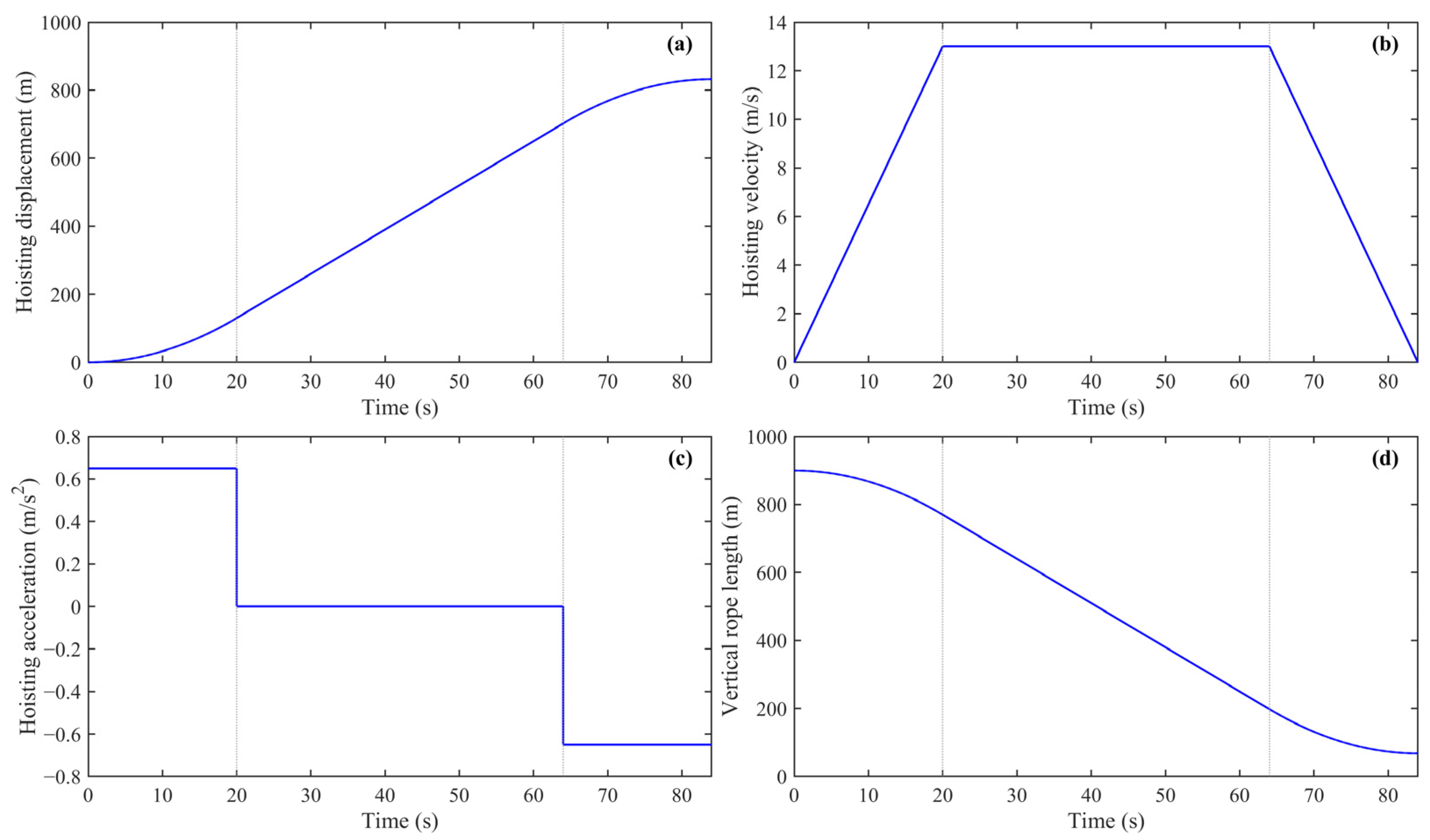
The nominal hoisting process follows a trapezoidal velocity profile consisting of acceleration, constant-speed, and deceleration stages. The conveyance accelerates during 0 ≤ t < 20 s, operates at the maximum hoisting speed during 20 ≤ t < 64 s, and decelerates during 64 ≤ t ≤ 84 s. The corresponding displacement, velocity, acceleration, and vertical rope-length variations are shown in Figure 3.

During the acceleration and deceleration stages, rapid variations in rope velocity and dynamic boundary excitation introduce significant transient tension fluctuations. Therefore, these two stages provide critical conditions for evaluating the safety-constrained balancing capability of the proposed controller.

5.1.2. Performance and Feasibility Indices

To quantify the tension-balancing performance and constraint satisfaction, the evaluation indices include the maximum absolute tension-imbalance ratio, the minimum safety margin, the cumulative boundary-violation duration, and the peak and RMS values of the dynamic inter-rope tension difference.

The maximum absolute total tension-imbalance ratio over the complete hoisting cycle is defined as

$$J_{\eta ,\max }={\max }_{0\le t\le t_f}\hspace{1em}|\eta (t)|,$$

(89)

where t_f denotes the end of the hoisting cycle.

The instantaneous safety margin is defined as

$$m_s(t)={\eta }_{\max }-|\eta (t)|,\hspace{1em}t\in [0,t_f].$$

(90)

A positive value of m_s(t) indicates that the instantaneous tension-imbalance state lies inside the prescribed safety boundary, whereas m_s(t) < 0 indicates an instantaneous boundary violation.

The minimum safety margin over the complete hoisting cycle is defined as

$$M_s={\eta }_{\max }-J_{\eta ,\max }.$$

(91)

A positive value of M_s indicates that the prescribed tension-imbalance constraint is satisfied throughout the complete hoisting cycle, whereas M_s < 0 indicates that at least one boundary violation occurs.

The cumulative boundary-violation duration is evaluated as

$$T_v={\displaystyle {\int }_0^{t_f}\mathbb{I}}\left(|\eta (t)|\ge {\eta }_{\max }\right)dt.$$

(92)

The RMS tension-imbalance ratio is defined as

$$J_{\tilde{\eta },\mathrm{RMS}}=\sqrt{{\displaystyle \frac{1}{t_f}}{\displaystyle {\int }_0^{t_f}{\tilde{\eta }}^2}(t)dt}.$$

(93)

The peak and RMS values of the dynamic inter-rope tension difference are defined as

$$J_{\Delta T,\max }={\max }_{0\le t\le t_f}|\Delta T_d(t)|.$$

(94)

$$J_{\Delta T,\mathrm{RMS}}=\sqrt{{\displaystyle \frac{1}{t_f}}{\displaystyle {\int }_0^{t_f}\Delta }{T}_d^2(t)dt}.$$

(95)

To quantify the activation of the attainable force projection and the corresponding constraint satisfaction during projection intervals, the projection–activation indicator is defined as

$${\chi }_p(t)=\left\{\begin{array}{ll}1,& |e_{Fa}(t)|>{\epsilon }_p\hfill \\ 0,\hfill & |e_{Fa}(t)|\le {\epsilon }_p\hfill \end{array}\right.,$$

(96)

where e_Fa(t) is the projection-induced differential-force correction, and ε_p is the numerical tolerance used to distinguish an active projection correction from numerical round off.

The projection time set is defined as

$${\mathcal{I}}_p=\{t\in [0,t_f]:{\chi }_p(t)=1\}.$$

(97)

The projection–activation ratio over the complete simulated hoisting cycle is calculated as

$$R_p={\displaystyle \frac{100}{t_f}}{\displaystyle {\int }_0^{t_f}{\chi }_p}(t)dt.$$

(98)

A larger value of R_p indicates that the nominal differential force exceeds the instantaneous attainable force interval for a larger proportion of the simulated cycle.

To evaluate constraint satisfaction specifically during the projection intervals, the minimum projection interval safety margin is defined as

$$M_{s,p}=\underset{t\in {\mathcal{I}}_p}{\min }\left[{\eta }_{\max }-\left|\eta \left(t\right)\right|\right].$$

(99)

A positive value of M_s,p indicates that no numerical tension-imbalance boundary violation occurs during the projection intervals. If ${\mathcal{I}}_j$ is empty, R_p = 0, and v is not applicable.

The uncontrolled, OPD, and BLF MRD cases are evaluated using identical mechanical parameters, hoisting profiles, and initial conditions. The projection related indices are applicable only to the BLF MRD case because the uncontrolled and OPD cases do not employ attainable force projection.

5.1.3. Optimized Passive Damping Benchmark

To provide a reproducible passive benchmark, two identical viscous dampers are placed at the same suspension locations as the two MRDs, while the load-bearing springs, mechanical parameters, hoisting profile, and initial equilibrium condition are kept unchanged. The passive damping force of the i-th suspension unit is defined as

$$F_{p,i}(t)=-c_p{\dot{x}}_{m,i}(t),\hspace{1em}i=1,2,$$

(100)

where the same constant damping coefficient c_p is used for both passive dampers. Following the optimization procedure in Ref. [16], c_p is determined offline by a parameter search under the nominal operating condition. Because the present study focuses on tension-imbalance safety and dynamic load sharing, the objective function is defined as

$$J_{\mathrm{OPD}}(c_p)=0.5{\displaystyle \frac{J_{\eta ,\max }(c_p)}{J_{\eta ,\max }(0)}}+0.5{\displaystyle \frac{J_{\Delta T,\mathrm{RMS}}(c_p)}{J_{\Delta T,\mathrm{RMS}}(0)}}.$$

(101)

The damping coefficient is searched over

$$c_p\in \left[0,c_{p,\max }\right],$$

(102)

with an increment of 10 N s/m. The admissible upper bound is selected to keep the passive damping force within a mechanical force level comparable to that attainable by the MRD system. The minimum objective value is obtained at

$$c_p^{\mathrm{opt}}=1.0\times {10}^4 \mathrm{N}\mathrm{s}/\mathrm{m}.$$

(103)

This value is kept fixed in all subsequent OPD simulations and is not retuned for different operating conditions. Because the OPD benchmark is purely passive, the MRD current limit, current slew rate, and current-driver dynamics are not applicable. The comparison therefore uses identical mechanical installation conditions while distinguishing the electrical constraints that apply only to the semi-active MRD system.

5.1.4. Conventional Sliding Mode MRD Benchmark

To provide a stronger semi-active benchmark, a conventional sliding mode controller is introduced for the dual-MRD system. This comparison is motivated by the sliding mode MRD strategy considered in Ref. [16]. Unlike the proposed BLF controller, the conventional sliding mode controller does not explicitly incorporate the prescribed tension-imbalance boundary into its control law.

Using the same differential-tension dynamics as the proposed controller, the sliding variable is defined as

$$s=\dot{\widehat{\eta }}+{\lambda }_s\widehat{\eta },$$

(104)

where $\widehat{\eta }$ denotes the dynamic tension-imbalance deviation from the static equilibrium. The nominal differential-force command is selected as

$$F_{d,\mathrm{SMC}}={\displaystyle \frac{1}{g_T}}\left[-f_T-{\lambda }_s\dot{\widehat{\eta }}-k_{s1}s-k_{s2}{\displaystyle \frac{s}{\left|s\right|+{\epsilon }_s}}\right].$$

(105)

The controller parameters are set to λ_s = 0.85 s⁻¹, k_s1 = 1.6 s⁻¹, k_s2 = 0.05 s⁻² and ε_s = 0.004 s⁻¹, and are kept unchanged throughout the comparison. To isolate the effect of the upper-level control law, the SMC MRD and BLF MRD cases use exactly the same dual-MRD hardware model, attainable force projection, force allocation, force-to-current inversion, current limit, current-driver dynamics, and slew-rate constraint.

5.1.5. Numerical Verification of the Differential-Force Effectiveness Coefficient

This subsection numerically verifies whether g_T(X, t) retains a known nonzero sign over the investigated operating envelope.

The numerical operating envelope includes the ranges of payload eccentricity, payload mass, hoisting acceleration, maximum hoisting speed, and allowable MRD current listed in

Table 3. Numerical bounds of the differential-force effectiveness coefficient over the investigated operating envelope.

Operating Factor	Evaluated Range	Min sggT	Max sggT	Sign of gT	Sign Change
Payload eccentricity (m)	0.04 to 0.08	9.42 × 10−4	1.38 × 10−2	Negative	No
Payload mass (kg)	30,000 to 50,000	6.49 × 10−4	2.05 × 10−2	Negative	No
Acceleration (m/s2)	0.50 to 0.80	9.37 × 10−4	1.40 × 10−2	Negative	No
Maximum speed (m/s)	9 to 13	9.42 × 10−4	1.38 × 10−2	Negative	No
Current limit (A)	0.6 to 1.6	9.41 × 10−4	1.38 × 10−2	Negative	No
Overall envelope	All cases	6.49 × 10−4	2.05 × 10−2	Negative	No

. These ranges are consistent with those used in the sensitivity analysis.

No sign reversal of g_T(X, t) was observed in any evaluated case. The coefficient remained negative throughout the investigated operating envelope, and hence sg = −1 was adopted. The numerical bounds of the sign normalized effectiveness coefficient were

$$-6.79\times {10}^{-4}\le s_g{g}_T(X,t)\le -2.05\times {10}^{-2} {\mathrm{kN}}^{-1}{\mathrm{s}}^{-2}.$$

Therefore, g_min = 6.79 × 10⁻⁴ > 0, confirming that the differential-force effectiveness coefficient remains bounded away from zero over the investigated operating envelope. The numerical verification supports the relative degree two model and the use of 1/g_T(X, t) in the nominal differential-force command.

5.1.6. Uncertainty Bound Estimation and Robust Gain Verification

The robust term in Equation (64) is introduced to compensate for bounded matched uncertainties arising from modeling errors, external disturbances, and differential-force-realization errors. In the present numerical implementation, the robust gain was selected as k_r = 0.05 s⁻² and was kept fixed throughout the nominal and sensitivity simulations.

The actuator-induced uncertainty was evaluated from the difference between the feasible target differential force and the actual differential force generated by the dual-MRD system. The corresponding equivalent contribution to the tension-imbalance acceleration channel remained bounded over the investigated numerical cases. In addition, robustness was assessed through prescribed mechanical-parameter mismatch and boundary-disturbance simulations.

The numerical results show that the selected gain provides sufficient robustness while maintaining actuator feasibility and positive tension-imbalance safety margins over the investigated operating conditions. These results provide numerical support for the selected robust gain. The resulting lumped uncertainty bound is ${\overline{\Delta }}_T$ = 0.03 s⁻², providing a positive robustness margin of 0.02 s⁻². Therefore, the gain condition required by Theorem 1 is satisfied over the investigated operating envelope during the no-projection intervals.

5.1.7. Modal Convergence and Reduced Model Fidelity

To assess the numerical adequacy of the reduced Galerkin model, a modal convergence study was conducted under the nominal operating condition, with N = 2, 4, 6, and 8 longitudinal modes per rope. To isolate modal truncation effects, the realized dual-MRD force histories from the nominal N = 4 closed-loop simulation were applied identically to all four models, while the mechanical parameters, hoisting profile, initial conditions, disturbances, and numerical solver settings were kept unchanged. The maximum absolute tension-imbalance ratio J_η,max, peak dynamic inter-rope tension difference, and RMS dynamic inter-rope tension difference were used as convergence indicators. The N = 8 solution was taken as the reference; the maximum relative deviation among the three indicators was used to quantify convergence. The results are summarized in

Table 4. Modal convergence of the reduced double-rope model under the nominal operating condition.

N	Jη,max	Peak |ΔTd|(kN)	RMS ΔTd (kN)	Maximum Relative Deviation
2	0.0176	1.270	0.251	20.62%
4	0.0171	1.104	0.208	1.30%
6	0.0171	1.101	0.208	0.24%
8	0.0170	1.087	0.208	0

.

As the retained order increases from N = 4 to N = 6 and N = 8, only minor changes are observed in the selected tension-response indices. Taking the N = 8 solution as the numerical reference, the maximum relative deviation in the N = 4 model among the three selected indices is 1.30%, while that of the N = 6 model decreases to 0.24%. These results indicate that the dominant longitudinal dynamics relevant to tension-imbalance regulation are adequately captured by four retained modes. Therefore, N = 4 modes per rope are used in the subsequent simulations to balance numerical accuracy and computational efficiency.

The numerical operating envelope includes the ranges of payload eccentricity, payload mass, hoisting acceleration, maximum hoisting speed, and allowable MRD current considered in the sensitivity analysis. Each factor was evaluated at three representative levels while the remaining factors were maintained at their nominal values, resulting in 15 one-factor-at-a-time operating cases. For each case, the complete hoisting cycle was simulated using the same controller structure and numerical settings.

In addition to the modal convergence test, the controller oriented reduced model is compared with an augmented reference model retaining a higher Galerkin order and the fixed length catenary-rope dynamics. Identical hoisting profiles, mechanical parameters, actuator forces, and initial conditions are used in the two models. The maximum absolute tension-imbalance ratio, peak dynamic inter-rope tension difference, and RMS dynamic inter-rope tension difference are used as comparison indices. The maximum relative differences between the reduced and reference models are 0.29%, 1.30%, and 0.40%, respectively. This supports the use of the reduced model over the investigated numerical operating envelope. The 10% tension-imbalance result should therefore be interpreted as a model-based safety result over the validated numerical operating envelope. Residual discrepancies between the reduced model and the higher fidelity reference are included in the modeling uncertainty used in the robust gain verification.

5.2. Nominal-Condition Tension-Balancing Performance

This section compares the nominal tension-balancing performance of the uncontrolled, OPD, SMC–MRD, and BLF–MRD cases. The total rope tensions, normalized tension-imbalance ratio, safety margin, and dynamic inter-rope tension difference are evaluated.

5.2.1. Tension Response and Safety Constraint Verification

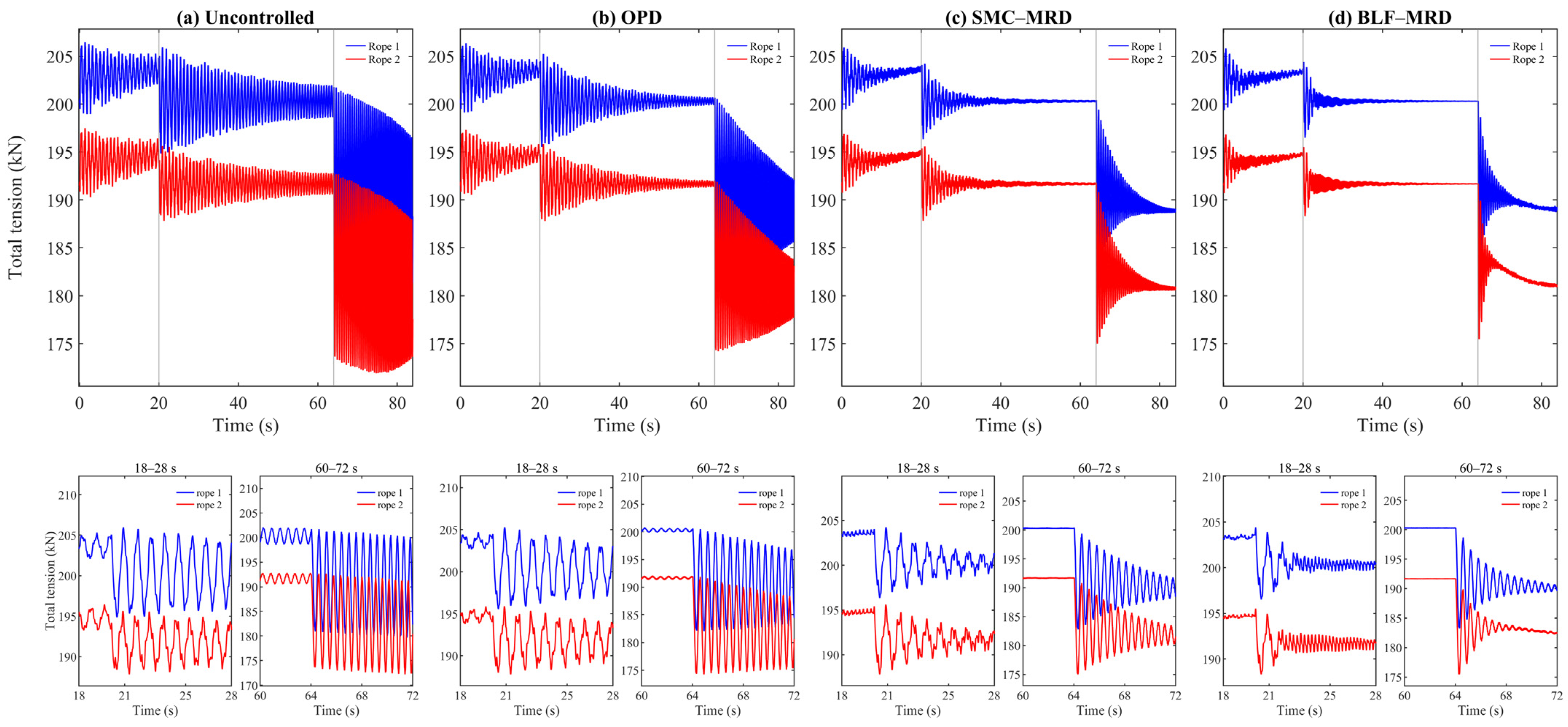
Figure 4 compares the total rope-tension responses of the uncontrolled, OPD, SMC–MRD, and BLF–MRD cases under the nominal operating condition.

In the uncontrolled case, the two rope tensions exhibit pronounced dynamic oscillations caused by the time-varying rope length, acceleration-induced excitation, and asymmetric load distribution. The inter-rope tension difference becomes particularly evident during the acceleration and deceleration stages, when changes in the hoisting motion produce strong transient responses. The OPD strategy attenuates part of the vibration by increasing the equivalent damping of the suspension units. However, because its damping action is not adjusted according to the instantaneous tension-imbalance state, its improvement in dynamic load sharing remains limited. The SMC–MRD strategy provides stronger vibration suppression than OPD and further reduces the inter-rope tension difference, although noticeable transient oscillations remain near the stage transitions. By contrast, the BLF–MRD strategy provides the smallest tension fluctuations and inter-rope tension differences over the complete hoisting cycle. Short transient responses remain near the stage-transition instants at t = 20 s and t = 64 s, but decay rapidly thereafter. The controlled responses retain the quasi-static tension offset associated with payload eccentricity while markedly reducing the superimposed dynamic oscillations.

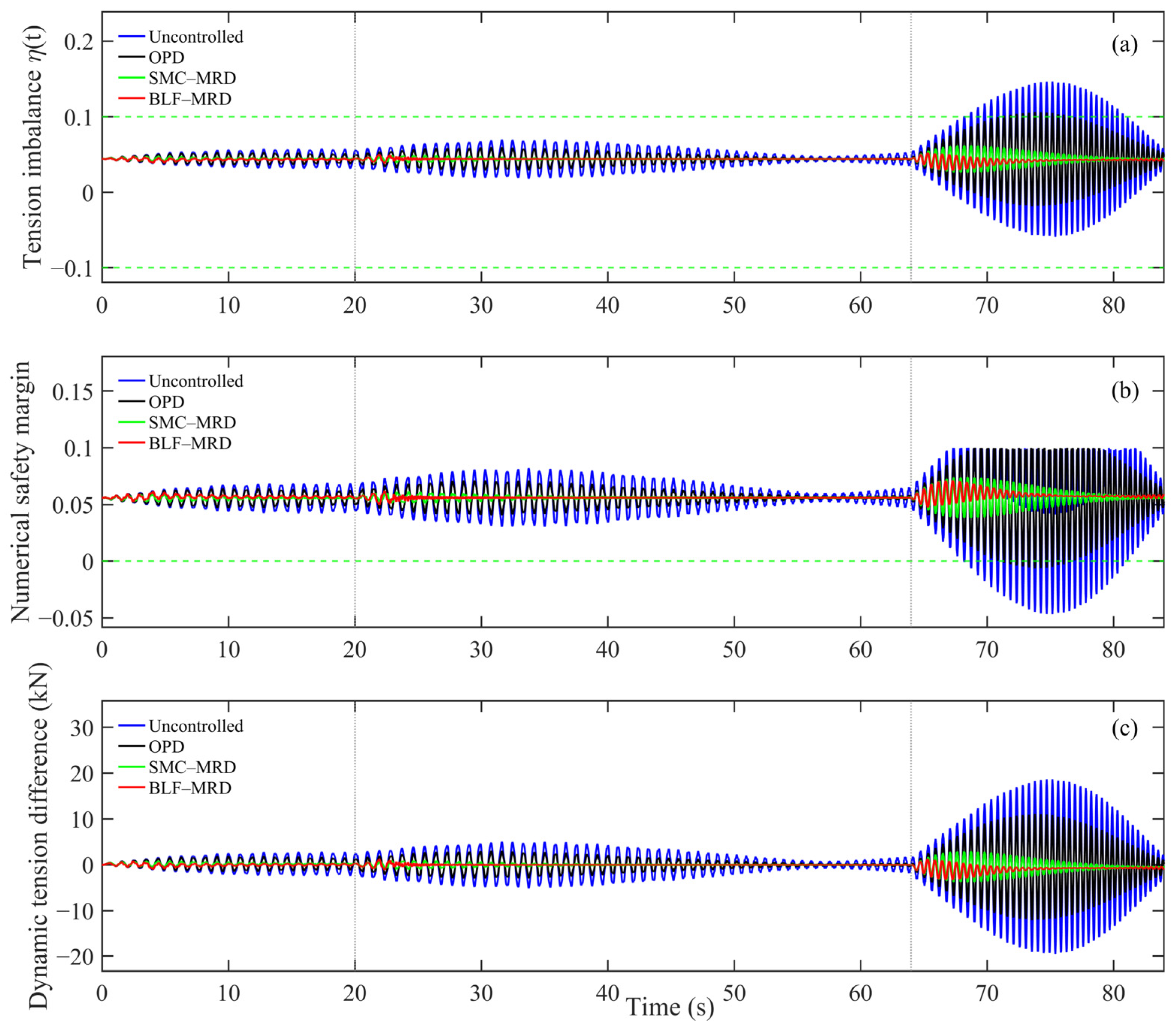
To further verify whether the dynamic tension regulation satisfies the prescribed safety requirement, the normalized tension-imbalance ratio is evaluated.

The results presented in Figure 5 indicate that the tension imbalance of the uncontrolled system exceeds the prescribed safety boundary. The imbalance increases significantly during transient operating stages, especially near the acceleration-to-constant-speed and constant-speed-to-deceleration transitions. The OPD strategy improves the response by reducing the imbalance oscillation amplitude. However, the safety boundary is still slightly exceeded. The SMC–MRD strategy provides further suppression and keeps the tension imbalance closer to the allowable region, although larger transient oscillations remain than in the BLF–MRD case. In contrast, the BLF–MRD-controlled response remains inside the allowable region throughout the complete hoisting cycle.

The quantitative performance comparison is summarized in

Table 5. Numerical evaluation of tension-imbalance constraint satisfaction under the nominal operating condition.

Control Strategy	${\mathit{J}}_{\mathit{\eta },\mathbf{max}}$	${\mathit{M}}_{\mathit{s}}$	${\mathit{T}}_{\mathit{v}}\left(\mathit{s}\right)$	Safety Status
Uncontrolled	0.1380	–0.0380	3.32	Violated
OPD	0.1064	–0.0064	1.01	Violated
SMC–MRD	0.0704	0.0296	0.00	Satisfied
BLF–MRD	0.0404	0.0596	0.00	Satisfied

. As shown in Table 5, the maximum absolute imbalance ratio of the uncontrolled system reaches J_η,max = 0.1380, which exceeds the prescribed numerical boundary. The OPD strategy reduces this value to J_η,max = 0.1064, but a boundary violation remains. The SMC–MRD strategy further reduces the maximum imbalance ratio to J_η,max = 0.0704, corresponding to a positive safety margin of 0.0296, and no boundary violation is observed. In the numerical simulation, the implemented BLF–MRD strategy limits the maximum imbalance ratio to J_η,max = 0.0404, corresponding to a reduction of approximately 70.7% relative to the uncontrolled case. No numerical boundary violation is observed during the complete simulated hoisting cycle, including the intervals in which feasibility projection is activated.

The key improvement is that the BLF formulation directly incorporates the tension-imbalance limit into the control design in this paper. When the imbalance state approaches the prescribed boundary, the barrier term increases the corrective differential-force demand, while the dual-MRD allocation mechanism converts this demand into physically feasible actuator forces. Although SMC–MRD also satisfies the prescribed constraint under the nominal condition, BLF–MRD provides a larger numerical safety margin and a lower maximum imbalance ratio. The proposed strategy improves dynamic load sharing and maintains the prescribed tension-imbalance constraint throughout the simulation.

5.2.2. Stage-Wise Quantitative Performance Evaluation

To evaluate the stage-dependent performance, the hoisting cycle is divided into acceleration, constant-speed, and deceleration stages. For each stage, the peak and RMS dynamic inter-rope tension differences are calculated to characterize transient severity and sustained oscillation intensity, respectively.

The absolute values and the corresponding reduction rates are presented in

Table 6. Stage-wise peak and RMS values of the dynamic inter-rope tension difference under the nominal operating condition.

Operating Phase	Control Strategy	${\mathit{J}}_{\mathbf{\Delta }\mathit{T},\mathbf{max}}\left(\mathbf{kN}\right)$	${\mathit{J}}_{\mathbf{\Delta }\mathit{T},\mathit{R}\mathit{M}\mathit{S}}\left(\mathbf{kN}\right)$	Peak Rates (%)	RMS Rates (%)
Acceleration	Uncontrolled	2.84	1.41	—	—
	OPD	1.73	0.82	39.2	41.7
	SMC–MRD	1.08	0.43	62.0	69.5
	BLF–MRD	0.97	0.26	65.8	81.6
Constant speed	Uncontrolled	5.12	2.37	—	—
	OPD	2.62	1.05	48.8	55.7
	SMC–MRD	1.35	0.42	73.6	82.3
	BLF–MRD	1.19	0.17	76.8	92.8
Deceleration	Uncontrolled	19.51	9.60	—	—
	OPD	10.42	4.97	46.6	48.2
	SMC–MRD	5.33	2.29	72.7	76.1
	BLF–MRD	1.89	1.12	90.3	88.3

. It shows that the dynamic inter-rope tension difference varies considerably among the three operating stages. The OPD, SMC–MRD, and BLF–MRD strategies all reduce the dynamic tension difference, with BLF–MRD consistently providing the lowest peak and RMS values. During acceleration, BLF–MRD reduces the peak and RMS values from 2.84 and 1.41 kN to 0.97 and 0.26 kN, respectively, while SMC–MRD reduces them to 1.08 and 0.43 kN. During constant-speed operation, the RMS value is reduced from 2.37 kN to 0.42 kN by SMC–MRD and further to 0.17 kN by BLF–MRD, indicating effective suppression of sustained oscillations. The most severe response occurs during deceleration, where the uncontrolled peak reaches 19.51 kN; SMC–MRD reduces it to 5.33 kN, whereas BLF–MRD further limits it to 1.89 kN.

To compare the relative effectiveness of the two damping strategies independently of the different absolute response levels in each stage, the reduction rate of a given performance index is defined as

$$R_J={\displaystyle \frac{J_{\mathrm{UC}}-J_{\mathrm{C}}}{J_{\mathrm{UC}}}}\times 100\%,$$

(106)

where J_UC and J_C denote the uncontrolled and controlled values, respectively.

Table 6 confirms a progressive improvement from OPD to SMC–MRD and BLF–MRD. For SMC–MRD, the peak reductions are 62.0%, 73.6%, and 72.7% during acceleration, constant-speed operation, and deceleration, respectively, with corresponding RMS reductions of 69.5%, 82.3%, and 76.1%. BLF–MRD provides still greater reductions, reaching 65.8%, 76.8%, and 90.3% in peak response and 81.6%, 92.8%, and 88.3% in RMS response. These results show that BLF–MRD provides the strongest overall suppression, particularly for sustained oscillations during constant-speed operation and severe transient responses during deceleration.

5.3. MRD Force Feasibility and Realization Performance

The results in Section 5.2 demonstrate the system-level tension-balancing performance of the proposed BLF–MRD strategy. However, the commanded differential force must be realized within the state-dependent force limits, current constraints, nonlinear MRD characteristics, and finite driver dynamics. Therefore, this section evaluates the actuator-realization process to determine whether the safety-constrained performance is preserved under actuator no idealities.

5.3.1. Differential-Force Feasibility and Projection

The upper-level BLF controller generates a nominal equivalent differential-force command according to the reconstructed tension-imbalance state. Because the force generated by each MR damper depends on its instantaneous relative displacement, relative velocity, and admissible current, the dual-MRD system provides a time-varying attainable differential-force interval. When the nominal command lies outside this interval, it is projected onto the nearest attainable boundary before force allocation.

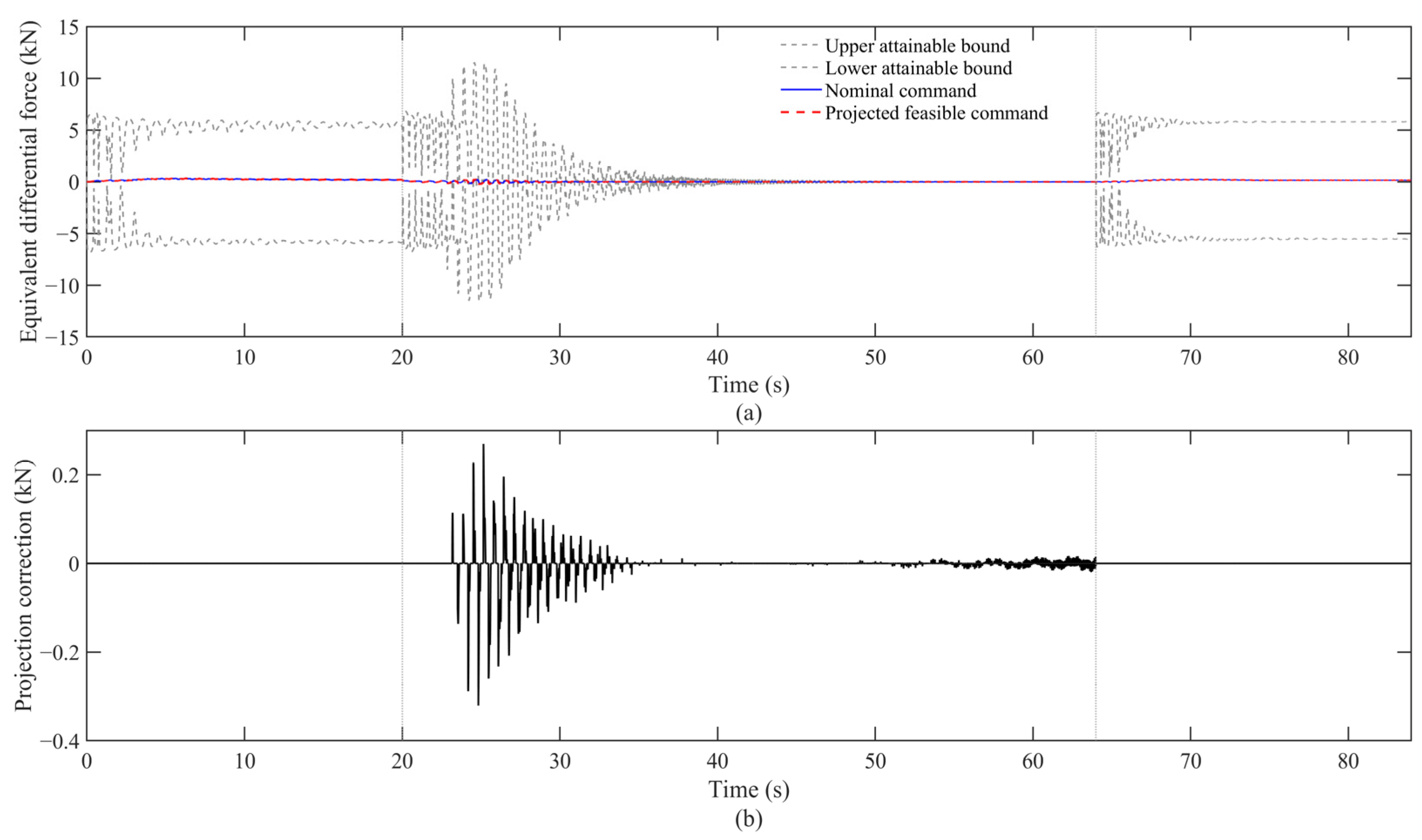
Figure 6 compares the nominal and projected differential-force commands with the instantaneous attainable bounds and presents the corresponding projection correction.

As shown in Figure 6a, the attainable differential-force interval varies continuously throughout the hoisting cycle. More pronounced variations occur near t = 20 s and t = 64 s, where changes in the operating-stage modify the relative displacement and velocity states of the two suspension units. These state variations directly alter the semi-active force capability of each MR damper and, consequently, the differential-force authority of the dual-MRD system. Figure 6b shows that projection is activated primarily during short transient intervals near the operating stage transitions. The projection–activation ratio is 6.1%, indicating that the nominal command is directly attainable during approximately 93.9% of the simulation period.

5.3.2. Commanded and Applied Currents

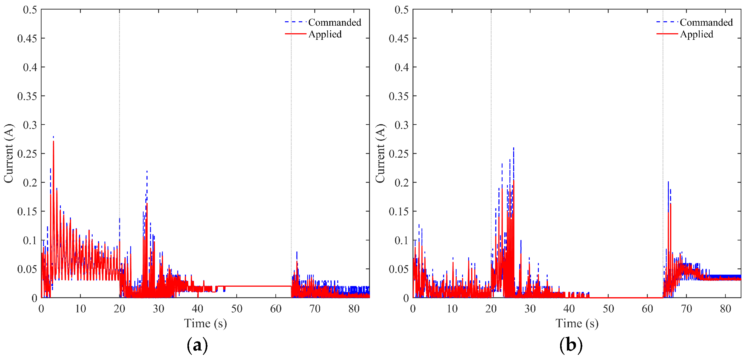
After the feasible differential-force command is allocated between the two MRDs, the individual target forces are converted into bounded current commands through the inverse MRD model. The actual coil currents are then generated by the rate-limited first-order current-driver dynamics. Figure 7 compares the commanded and applied currents of the two MRDs.

The applied currents generally follow their corresponding commands over the complete hoisting cycle in Figure 7. Small amplitude attenuation and phase lag appear during rapid command variations, particularly near the operating-stage transitions at t = 20 s and t = 64 s. These deviations result from the finite driver time constant and current slew-rate constraint, rather than from failure of the inverse force-to-current mapping.

The maximum applied currents of MRD 1 and MRD 2 are 0.2818 and 0.2605 A, respectively, which are substantially below the prescribed maximum current of 1.6 A. Moreover, no current saturation occurs during the simulation. These results indicate that the nominal tension-balancing task does not require persistent operation near the physical current limit. Although the applied currents remain well below I_max, feasibility projection can still occur because the instantaneous differential-force authority is also restricted by the suspension-motion states and the semi-active dissipativity condition.

During most of the constant-speed stage, the current demand remains relatively small because the controller mainly compensates for residual oscillations caused by the variable-length rope dynamics. The current histories of the two MRDs are not identical because the constrained allocation method distributes the required differential-force effect according to their instantaneous force capabilities and motion states. This asymmetric current allocation is therefore an expected consequence of differential-force regulation rather than inconsistent actuator operation.

5.3.3. Target and Realized MRD Forces

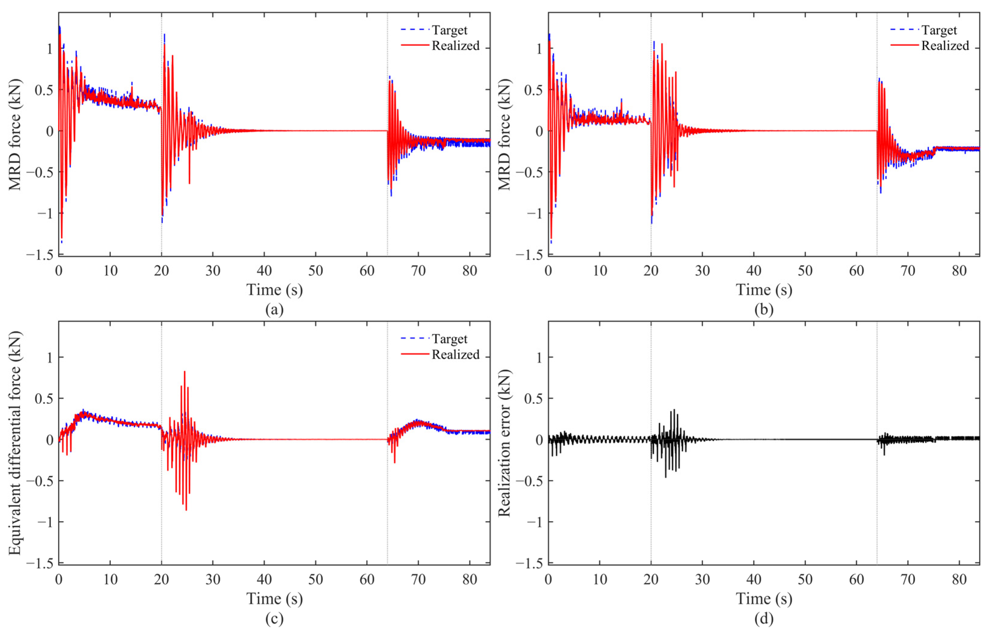
Figure 8 evaluates the final stage of the actuator-realization process. The individual target forces are compared with the forces generated by the nonlinear MRD models, while the feasible and realized equivalent differential forces are used to assess the combined force-tracking performance of the dual-MRD system.

As shown in Figure 8a,b, the realized forces of both MRDs closely follow their allocated target forces during most of the hoisting cycle. The largest deviations occur near t = 20 s and t = 64 s, where the target forces change rapidly in response to the stage-transition excitation. Because the applied currents cannot change instantaneously, the combined effects of current-driver lag, slew-rate limitation, and nonlinear MRD hysteresis produce short-duration force-tracking errors.

Figure 8c confirms that the realized equivalent differential force follows the feasible target over the complete simulation. Figure 8d further shows that the realization error is concentrated mainly around the operating-stage transitions and remains small during the slowly varying portions of the motion. The peak differential-force-realization error is 0.4407 kN, whereas its RMS value is only 0.0225 kN. The large difference between the peak and RMS values indicates that the principal realization errors are brief transient events rather than persistent tracking offsets.

The different force histories of MRD 1 and MRD 2 arise from the constrained force-allocation process under eccentric static load sharing. The individual forces are not required to be equal; instead, their combined effect must reproduce the feasible equivalent differential-force demand while satisfying the instantaneous semi-active force constraints. The quantitative actuator-feasibility and realization indices are summarized in

Table 7. Quantitative actuator-feasibility and force-realization indices under the nominal operating condition.

Index	MRD1	MRD2	Combined/Differential
Maximum applied current (A)	0.2818	0.2605	—
RMS applied current (A)	0.0379	0.0259	—
Current-tracking RMSE (A)	0.0063	0.0064	—
Current-saturation ratio (%)	0	0	0
Projection–activation ratio (%)	—	—	6.1
Peak projection correction (kN)	—	—	0.4045
RMS projection correction (kN)	—	—	0.0178
Minimum safety margin during projection	—	—	0.0737
Peak differential-force error (kN)	—	—	0.4407
Differential-force RMSE (kN)	—	—	0.0225

.

Overall, the actuator-level results show that the applied currents remain within the prescribed range, no current saturation occurs, and the differential-force-realization error is confined mainly to short intervals near the operating-stage transitions. The prescribed tension-imbalance constraint also remains satisfied numerically when state-dependent semi-active force limits, feasibility projection, nonlinear MRD force–current characteristics, current-driver dynamics, and hysteresis are included. However, since feasibility projection is active during 6.1% of the simulated cycle, the complete-cycle constraint satisfaction should be interpreted as a numerical result, whereas the strict theoretical guarantee applies to the no-projection intervals.

5.4. Sensitivity Analysis Under Operating and Actuator Variations

Robustness is evaluated through a factor-by-factor sensitivity study in which payload eccentricity, payload mass, hoisting acceleration, maximum speed, and the allowable MRD current are varied about the nominal condition. For each level, the uncontrolled and BLF–MRD responses are compared under the same constraint, |η| ≤ η_max.

5.4.1. Effect of Payload Eccentricity

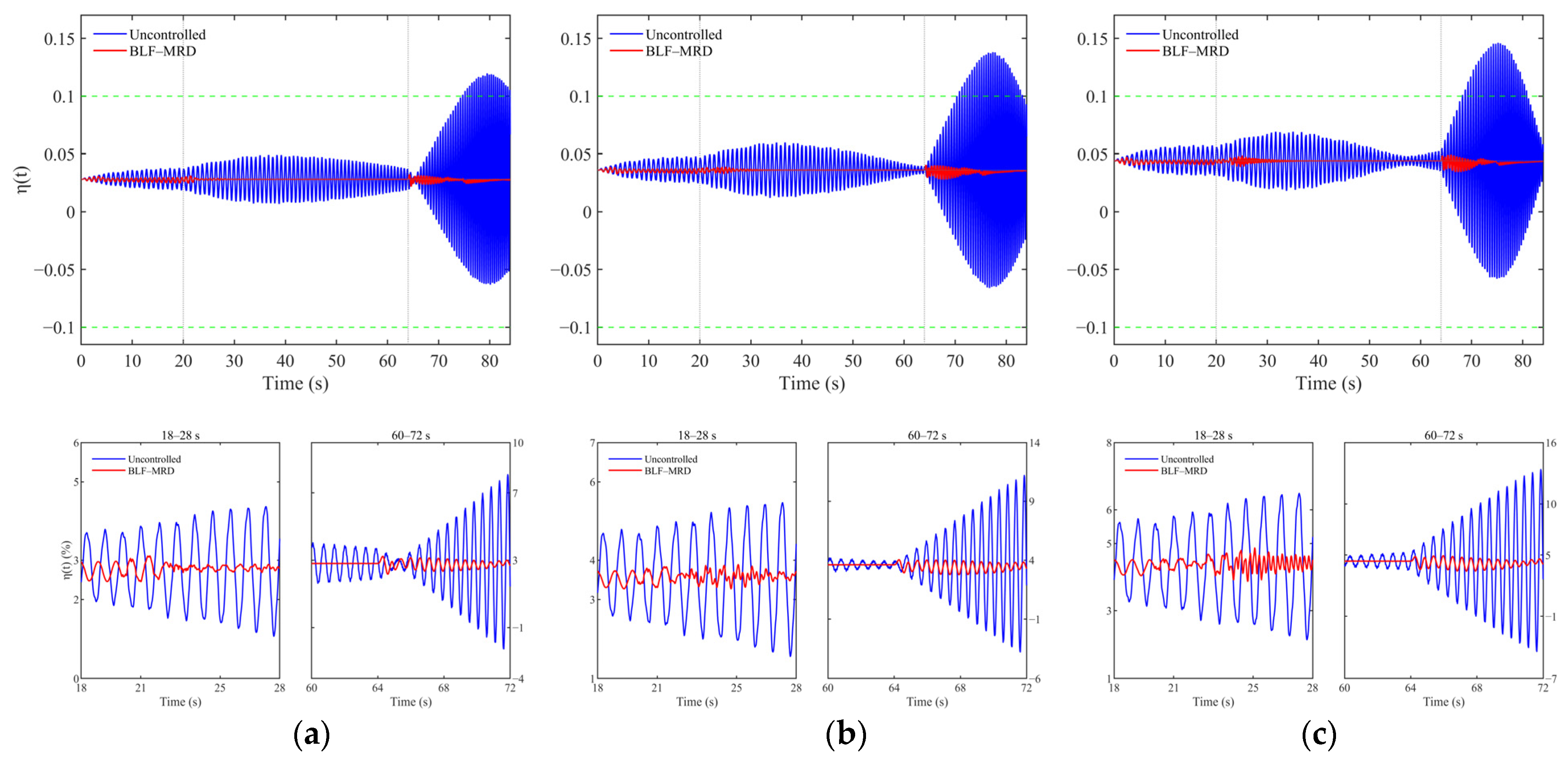
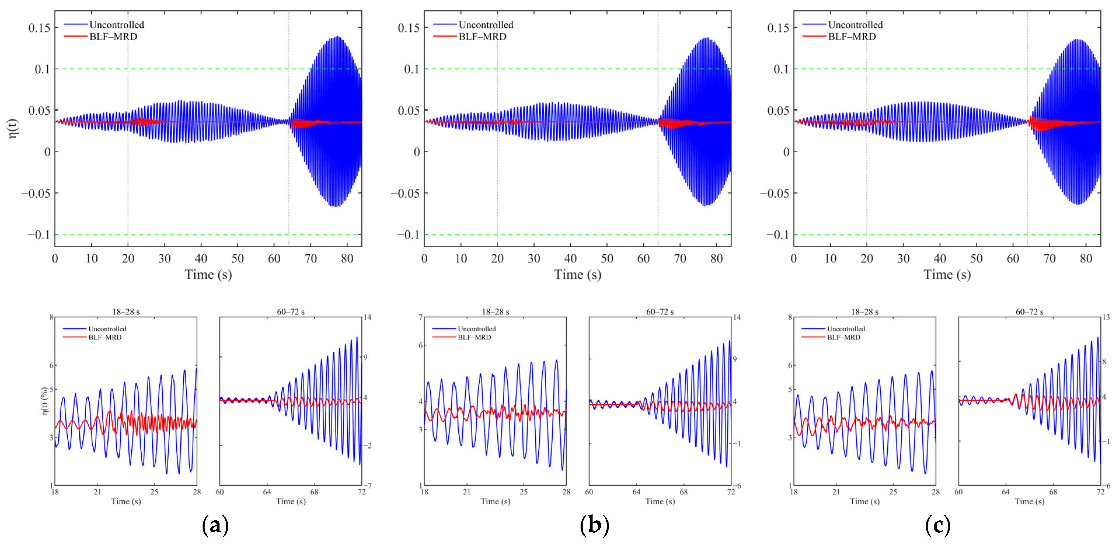
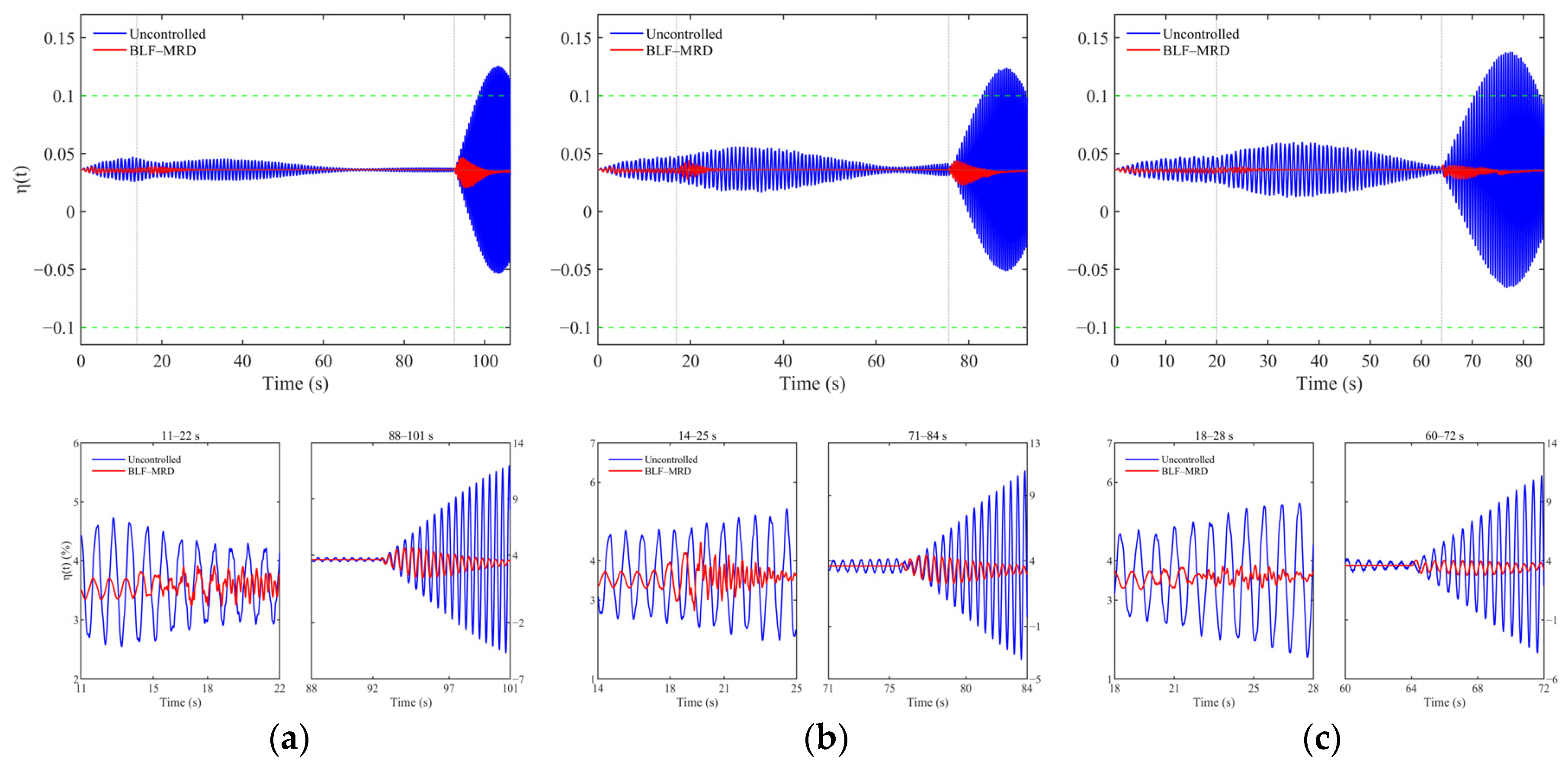
Payload eccentricity changes the static load-sharing difference between the two ropes and shifts the equilibrium tension-imbalance state relative to the prescribed safety boundary. Figure 9 compares the uncontrolled and BLF–MRD-controlled responses for eccentricities of 0.04, 0.06, and 0.08 m.

In the uncontrolled cases, the tension-imbalance ratio oscillates around an eccentricity-dependent nonzero equilibrium. As the eccentricity increases, the equilibrium position moves closer to the upper safety boundary, and the transient oscillations become more pronounced, particularly during the deceleration stage. This behavior indicates that a larger eccentricity leaves less available margin for accommodating dynamic disturbances. The BLF–MRD strategy substantially suppresses the oscillatory component and maintains the controlled response within the prescribed boundary at all three eccentricity levels. Nevertheless, the controlled equilibrium also shifts toward the boundary as the eccentricity increases. Payload eccentricity is therefore a primary factor governing the residual safety margin and should be restricted when defining the admissible loading configuration.

5.4.2. Effect of Payload Mass

The eccentricity-to-suspension-spacing ratio remains unchanged, varying the payload mass does not directly alter the normalized static load-sharing relationship. Figure 10 compares the tension-imbalance responses for payload masses of 30,000, 40,000, and 50,000 kg.

The uncontrolled responses exhibit similar normalized imbalance levels over the investigated mass range, although differences in the transient oscillations remain visible near the operating-stage transitions. This relatively weak variation is partly associated with the normalization by the total rope tension, which increases with payload mass. Under BLF–MRD control, all three responses remain within the prescribed safety boundary, and their overall time-history characteristics are only moderately affected by payload mass. However, a larger payload increases the absolute inertial loading and may intensify the dynamic inter-rope tension difference even when the normalized imbalance changes only slightly. Payload mass should therefore be evaluated using both normalized safety indices and absolute tension-difference indices.

5.4.3. Effect of Hoisting Acceleration

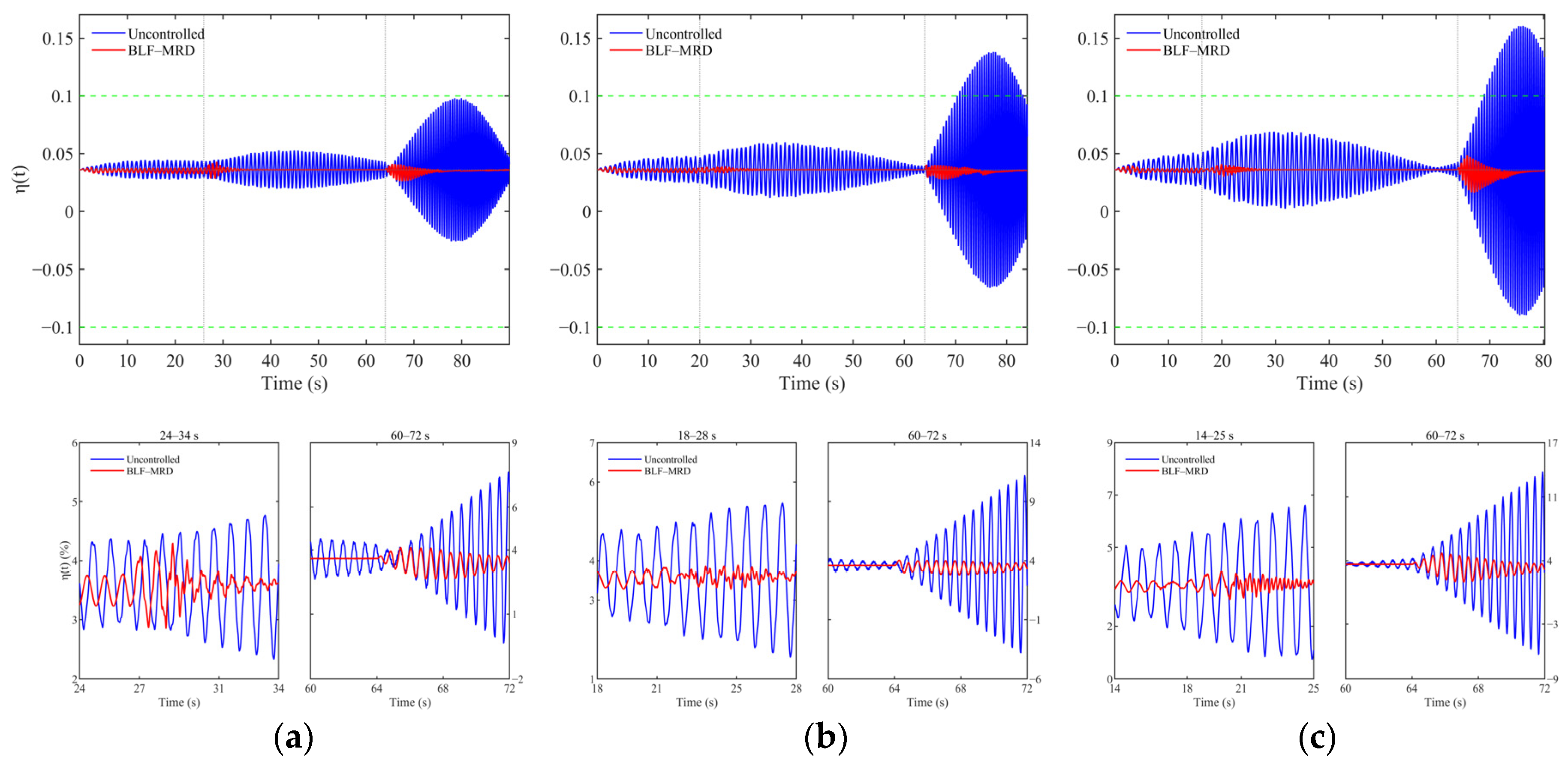
Hoisting acceleration determines the inertial excitation applied to the conveyance and ropes and is therefore expected to have a direct influence on the transient tension response. Figure 11 compares the responses for accelerations of 0.50, 0.65, and 0.80 m/s².

In the uncontrolled system, increasing the acceleration intensifies the transient tension oscillations, especially near the operating-stage transitions. The response becomes most pronounced after the onset of deceleration, where the abrupt change in acceleration excites the longitudinal dynamics of the variable-length ropes. The BLF–MRD strategy effectively attenuates these transient oscillations and maintains the tension imbalance within the allowable region at all three acceleration levels. However, higher acceleration produces a stronger controlled response and increases the required differential-force authority. Hoisting acceleration is therefore a dominant parameter governing transient dynamic loading and should be selected by balancing transportation efficiency, rope-load suppression, and actuator capability.

5.4.4. Effect of Maximum Hoisting Speed

In the adopted simulations, the total lifting distance is maintained while the motion-stage durations vary with the selected maximum speed. Therefore, the results reflect the combined influence of maximum speed and motion-profile duration. Figure 12 compares the responses for maximum hoisting speeds of 9, 11, and 13 m/s.

The uncontrolled response does not vary monotonically with maximum speed. Changes in the stage durations alter the rope-length trajectory, the time spent in each operating stage, and the instant at which the system encounters transition-induced excitation. Consequently, a lower maximum speed does not necessarily produce a smaller dynamic response. The BLF–MRD strategy maintains the controlled imbalance within the prescribed boundary for all three speed profiles. The differences among the controlled responses are associated mainly with the duration and timing of the transient oscillations rather than with maximum speed alone. Maximum hoisting speed should therefore be assessed together with acceleration, stage duration, transition smoothness, and rope-length evolution.

5.4.5. Effect of the Maximum Allowable MRD Current

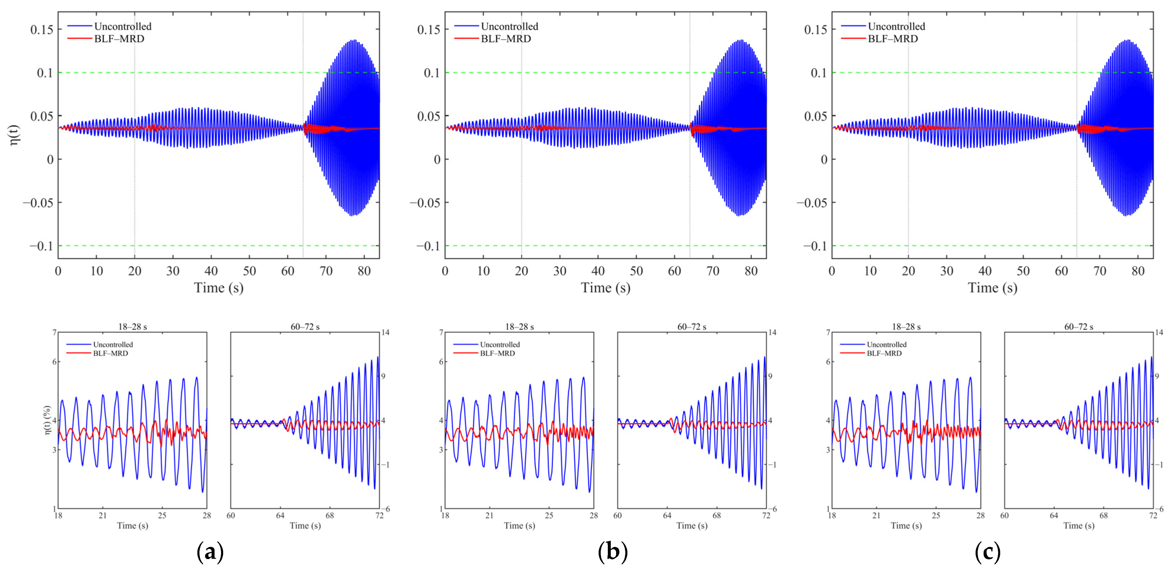
The maximum allowable current determines the attainable force range of each MR damper. Figure 13 compares current limits of 0.60, 1.00, and 1.60 A. The uncontrolled response remains unchanged because it is independent of the available MRD current.

The controlled tension-imbalance histories remain similar over the investigated current range, and the prescribed safety boundary is satisfied in all three cases. This result indicates that the examined current limits provide sufficient control authority to maintain the system-level safety requirement under the considered operating condition. Increasing the allowable current generally enlarges the attainable force set. Once sufficient force authority is available, further increases in current capacity produce only limited changes in the system-level tension response. The current limit should therefore be selected by considering both the required safety performance and the desired actuator-feasibility reserve.

5.4.6. Overall Sensitivity Comparison

The parameter values are specified in the time-history comparisons, whereas the corresponding system-level performance indices are summarized in

Table 8. Overall sensitivity of the tension-imbalance safety and dynamic tension-balancing performance to operating and actuator parameters.

Varied Factor	Level	${\mathit{J}}_{\mathit{\eta },\mathbf{max}}^{\mathit{U}\mathit{C}}$	${\mathit{M}}_{\mathit{s}}^{\mathit{B}\mathit{L}\mathit{F}}$	${\mathit{J}}_{\tilde{\mathit{\eta }},\mathit{R}\mathit{M}\mathit{S}}^{\mathit{B}\mathit{L}\mathit{F}}$	${\mathit{J}}_{\mathbf{\Delta }\mathit{T},\mathbf{max}}^{\mathit{B}\mathit{L}\mathit{F}}\left(\mathbf{kN}\right)$
Payload eccentricity	0.04 m	0.1197	0.0677	0.00122	1.29
	0.06 m	0.1380	0.0596	0.00163	1.89
	0.08 m	0.1461	0.0506	0.00182	2.22
Payload mass	30,000 kg	0.1399	0.0588	0.00160	1.88
	40,000 kg	0.1380	0.0596	0.00163	1.89
	50,000 kg	0.1361	0.0567	0.00215	2.78
Acceleration	0.50 m/s2	0.0980	0.0571	0.00187	2.08
	0.65 m/s2	0.1380	0.0596	0.00163	1.89
	0.80 m/s2	0.1604	0.0514	0.00296	4.06
Maximum speed	9 m/s	0.1259	0.0532	0.00210	3.36
	11 m/s	0.1241	0.0553	0.00216	2.89
	13 m/s	0.1380	0.0596	0.00163	1.89
Maximum allowable current	0.6 A	0.1380	0.0586	0.00161	1.76
	1.0 A	0.1380	0.0577	0.00149	2.03
	1.6 A	0.1380	0.0596	0.00163	1.89

.

The results summarized in Table 8 show that the BLF–MRD strategy maintains a positive safety margin for all investigated parameter levels. Payload eccentricity has the greatest influence on the residual safety margin, whereas hoisting acceleration most strongly affects the transient dynamic response. Payload mass mainly changes the absolute inter-rope tension difference, while the effect of maximum hoisting speed is non-monotonic because it also alters the stage durations and rope-length trajectory. Variations in the allowable MRD current produce only minor changes in the system-level indices, indicating that the available current capacity is sufficient within the investigated range.

5.5. Integrated Discussion and Engineering Implications

Taken together, the results indicate that the available dynamic safety margin is governed by both the eccentricity-induced operating equilibrium and the transient tension demand. Increasing payload eccentricity reduces the residual margin available for dynamic regulation, whereas variations in hoisting acceleration and speed mainly affect the transient differential-force demand. Therefore, payload centering and motion profile design should be considered jointly when defining safe operating conditions.

At the actuator level, the state-dependent feasibility projection and constrained force allocation prevent unattainable differential-force commands from being transmitted directly to the MRDs. Under the nominal operating condition, projection is activated during 6.1% of the simulated hoisting cycle, while the nominal command is directly attainable during approximately 93.9% of the cycle. The differential-force tracking RMSE is 0.0225 kN. Projection corrections occur mainly near the operating-stage transitions, where rapid changes in suspension motion temporarily reduce the available differential force authority. The projection results also clarify the scope of the analytical guarantee. During the projection intervals, the simulated tension imbalance remains within the prescribed boundary, providing numerical evidence of constraint satisfaction rather than a strict analytical guarantee. For the no-projection intervals covered by Theorem 1, the quantified uncertainty budget further shows that the selected robust gain exceeds the conservative lumped uncertainty bound over the investigated operating envelope. Thus, the numerical controller parameters satisfy the gain condition required by the strict stability analysis.

The sensitivity results provide a basis for defining an admissible operating envelope. Payload eccentricity should be limited to preserve sufficient residual safety margin, while acceleration and velocity profiles should be selected to reduce transient force demand. Increasing the allowable MRD current alone may provide limited additional benefit unless the suspension-motion states and semi-active force constraints are considered simultaneously. Although the actuator model has been experimentally validated in previous work, the complete dual-MRD closed-loop control framework has not yet been verified on a double-rope hoisting test platform. Therefore, the present results demonstrate numerical feasibility but do not fully establish practical effectiveness under sensor noise, structural mismatch, communication delay, and unmodeled hardware dynamics.

The reliability of the numerical results is assessed from several complementary aspects. First, the nonlinear MRD model and its constitutive coefficients are adopted from an experimentally identified actuator model reported in Ref. [16]. Second, modal convergence is examined by increasing the retained Galerkin order from N = 4 to higher orders, and the resulting changes in the principal tension-response indices remain within 1.30%. Third, reducing the numerical integration step by one half changes the maximum tension-imbalance ratio and RMS dynamic inter-rope tension difference by only 0.019% and 0.283%, respectively. Finally, the sensitivity analyses demonstrate that the main conclusions remain consistent over the investigated variations in payload eccentricity, payload mass, hoisting acceleration, maximum speed, and allowable MRD current. These checks support the numerical consistency of the reported results. However, they do not constitute experimental validation of the complete dual-MRD-controlled hoisting system.

6. Conclusions

This study developed a safety-constrained semi-active differential-tension control framework for a variable-length double-rope mine hoist equipped with dual-MRDs. The framework combines a BLF-based robust backstepping controller with state-dependent force feasibility, constrained dual-MRD allocation, force-to-current inversion, and current-driver dynamics, thereby integrating tension-imbalance regulation with physically realizable actuator commands.

Under the explicit control authority condition, the closed-loop error signals remain bounded, and the prescribed tension-imbalance safe set is forward invariant over any interval during which the nominal differential force remains inside the instantaneous attainable set. The modeling, external disturbance, and force-realization contributions were quantified over the investigated operating envelope, and the selected robust gain was verified to exceed the resulting conservative lumped uncertainty bound used in the no-projection stability analysis. The proposed controller substantially improves load-sharing performance, achieving a tension imbalance well below the prescribed safety limit under the nominal condition. Sensitivity simulations also maintain positive numerical safety margins under all investigated variations in payload eccentricity, payload mass, hoisting acceleration, maximum hoisting speed, and allowable MRD current.

These results indicate that the proposed framework can improve dynamic load sharing while preserving the eccentricity-induced static load-sharing condition. The numerical consistency of the results is supported by the experimentally identified MRD model, convergence checks, and sensitivity analyses. Nevertheless, the present study is limited to numerical validation, and the experimentally identified MRD model does not constitute system-level validation of the complete dual-MRD control framework. Moreover, the strict forward invariance result applies only to intervals without feasibility projection, while complete-cycle constraint satisfaction is supported numerically within the investigated operating envelope. Future work will incorporate projection effects into the theoretical analysis and conduct hardware in the loop and scaled hoisting experiments considering measurement, estimation, delay, driver, and modeling uncertainties.