An Adaptive Fixed-Time Dynamic Triggered Control for Interconnected Power Systems Under Denial-of-Service Attacks

Abstract

In this work, an adaptive fixed-time dynamic triggered control issue for interconnected power systems under Denial-of-Service (DoS) attacks is investigated. Such attacks would impede the transmission of sensor signals in interconnected power systems, precipitating a severely unstable power supply or even paralysis. To effectively confront this challenge, an adaptive switching neural network state observer is designed. The observer can maintain the output of the observation state under both attack conditions and normal conditions, thereby compensating for the adverse effects of DoS attacks on interconnected power systems. Meanwhile, a nonlinear fixed-time filter is constructed, which not only obviates the complexity explosion issue but also enhances the convergence capability of interconnected power systems. Moreover, a dual dynamic parameter threshold Event-Triggered Mechanism (ETM) is developed. Influenced by multiple dynamic parameters, this mechanism achieves a more precise control of triggered conditions, drastically conserving the communication resources of the interconnected power systems and preventing the occurrence of Zeno behavior. Ultimately, the effectiveness of the proposed methods is demonstrated by the simulation results.

1. Introduction

The stability control problems of power systems have been extensively researched in the past, including sliding mode control [1], $H_{\infty }$ control [2], model predicted control [3], and so on. However, the advancement of new energy technologies and the increase in diverse load equipment have led to the continuous expansion of the scale of modern power systems in recent years, whose structure becomes highly nonlinear, complex, and interconnected. This trend presents new challenges to the stability and control capabilities of power systems [4]. Therefore, optimizing the stability control strategies of power systems has become particularly important. In order to achieve transient stability enhancement, a nonlinear control strategy for a static synchronous series compensator and a doubly-fed induction generator within a multi-machine power system was presented in [5]. A power system stabilizer design approach based on the whale optimization algorithm was proposed for modified single-machine infinite bus and multi-machine systems in [6], aiming to improve the small-signal stability of the power system. In addition, disturbance-estimation-based robust control and integral sliding-mode control provide effective ways to improve disturbance rejection and robustness against uncertainties, which also offer useful insights for observer-based compensation design [7]. Clearly, the stability control strategies are continuously advancing.

On the basis of the progress made in stability control strategies, it is also necessary to recognize the vulnerability of modern power systems to external threats. In practical engineering, interconnected power systems are vulnerable to malicious attacks that pose threats to their stability [8]. DoS attacks, as one of the common types of network malicious attacks, disrupt data exchange between system components by interfering with communication channels, leading to the inability to use data from sensors or controllers normally [9]. Consequently, the issue of security control in power systems is garnering increasing attention. A methodology based on switching systems was proposed to the load frequency control scheme of a multi-area power system in [10], enhancing their resilience against DoS attacks. An innovative distributed fuzzy load frequency control strategy was propounded for power systems subjected to cross-layer random DoS attacks in [11]. To mitigate the damage caused by DoS attacks, it is highly meaningful to establish appropriate control strategies.

Backstepping control methods [12,13] are widely applied to complex nonlinear systems. It should be noted that when applying backstepping control methods, the virtual control laws need to be repeatedly differentiated, which may lead to the problem of complexity explosion, namely, increasingly complicated analytical expressions in the recursive controller design [14,15]. To address this, dynamic surface control technology has been proposed to improve traditional backstepping control methods [16,17]. Meanwhile, due to the potential difficulties in designing controllers for nonlinear systems, considering the outstanding approximation capabilities of neural networks [18], for unknown terms, many adaptive neural network control methods have been applied in [19]. When the system state variables are either unknown or partially known, it is necessary to estimate them through the state observer [20]. A novel neural network state observer was constructed in [21], which can acquire the required states from the nonlinear interconnected large-scale systems under DoS attacks. A dynamic state observer was developed for a multi-area interconnected power system to perform state estimation in [22].

Power systems, as critical infrastructures, have stringent requirements for time performance [23]. Therefore, achieving control objectives within a finite time is crucial. To guarantee the stability of nonlinear power systems with actuator faults and time delays, an adaptive fuzzy finite-time control scheme was designed in [24]. A finite-time fault-tolerant controller was proposed in [25], which make the tracking errors converge to a small neighborhood of the origin in finite time. However, in finite-time control strategies, the bounds on convergence time must rely on the initial state [26]. When the initial state is often unknown in practice, it becomes impossible to accurately determine the convergence time. Therefore, the fixed-time control method was proposed in [27,28,29]. A rapid fixed-time backstepping controller was designed to stabilize the DC microgrid in [30]. To enhance transient stability, a distributed hierarchical fixed-time frequency control structure was formulated in [31]. Obviously, studying the secure control of power systems within a fixed control framework is more practical.

In addition to this, as the scale of power systems increases and a large number of measurement devices are interconnected, it places a tremendous burden on the communication networks of power systems [32,33]. A way to maintain the speed of the power system while reducing redundant interactions has become a challenging issue. To conserve the network resources of interconnected synchronous generators, a decentralized dynamic ETM was devised in [34]. In addition, dynamic event-triggered adaptive fixed-time practical tracking control through funnel functions and prescribed-time dynamic event-based adaptive tracking control have also been investigated for uncertain nonlinear systems in [35,36]. An event-triggered consensus strategy was formulated for achieving consensus in interconnected two-time-scale systems with structured uncertainty in [37]. A decentralized periodic event-triggered scheme was designed to determine the time instants for transmitting the control signal to the equivalent generating unit in [38], which avoided Zeno behavior. A novel self-triggered protocol was proposed in [39], which eliminates the need for special hardware devices to continuously monitor the system state, thereby further conserving communication resources. Therefore, designing an appropriate event-triggering strategy to ensure the rapid convergence of the system while saving communication resources is necessary.

Inspired by the aforementioned literature, the adaptive fixed-time dynamic triggered control for interconnected power systems is investigated, and the main innovations are outlined as follows:

(1)

Compared to the existing results in [1,23,24,25,30,31], an adaptive switching neural network state observer is designed to compensate the adverse effects of DoS attacks on interconnected power systems. Through using neural networks to approximate unknown dynamics and employing switching logic to handle abrupt changes in sensor data under different conditions, it achieves the effective observation of the system state under both attack conditions and normal conditions, ensuring the stability of power supply.

(2)

Based on the construction of the nonlinear fixed-time filter, a dual dynamic parameter threshold ETM is developed. Different from the ETM in [22,32,33,34,37,38,39], the controller can more flexibly adjust the conditions for triggered events according to the actual operating state of the system, while ensuring the rapid recovery capability of the interconnected power system under DoS attacks. Correspondingly, the computational and communication resources of interconnected power systems are conserved and Zeno behavior is avoided.

The subsequent sections are organized as follows. Preliminaries and problem formulation are represented in Section 2. The controller design and system analysis for adaptive fixed-time dynamic triggered control under DoS attacks are represented in Section 3. Simulation results are represented in Section 4. Ultimately, the conclusion is represented in Section 5.

2. Preliminaries and Problem Formulation

2.1. Model Description

Consider a interconnected system composed of multiple interconnected generators. The phase and frequency of the power system are influenced by the angle and relative rotor speed of the synchronous generators, which are regulated by the excitation circuits of the synchronous generators.

The model of the interconnected system is formulated as follows:

$$\left\{\begin{array}{cc}\hfill {\dot{\theta }}_p\left(t\right)=& {\omega }_p\left(t\right),p=1,2,···,M\hfill \\ \hfill {\dot{\omega }}_p\left(t\right)=& -{\displaystyle \frac{D_p}{2I_p}}{\omega }_p\left(t\right)+{\displaystyle \frac{{\omega }_0}{2I_p}}[P_{mp}\left(t\right)-P_{ep}T\left(t\right)]\hfill \\ \hfill {\dot{P}}_{mp}\left(t\right)=& {\displaystyle \frac{1}{T_p}}[u_{gp}\left(t\right)-P_{mp}\left(t\right)]\hfill \\ \hfill P_{ep}\left(t\right)=& E_p{\displaystyle \sum _{q=1,q\ne p}^M}{E}_q[B_{pq}sin{\theta }_{pq}\left(t\right)+G_{pq}cos{\theta }_{pq}\left(t\right)]\hfill \end{array}\right.$$

(1)

where the physical meaning of the system parameters are given in the

Table 1. Physical meanings of system parameters.

Parameter	Physical Meaning
${\theta }_p$	Power angle of the p-th generator
${\omega }_p$	Relative rotor speed of the p-th generator
$u_{gp}$	Control signal for the p-th generator
$P_{mp}$	Mechanical power
$P_{ep}$	Electrical power
$D_p$	Damping coefficient
$I_p$	Inertia coefficient
$T_p$	Governor time coefficient
$E_p$	Transient electromotive force coefficient
$B_{pq}$	Imaginary part of the admittance matrix
$G_{pq}$	Real part of the admittance matrix

, with ${\theta }_{pq}\left(t\right)={\theta }_p\left(t\right)-{\theta }_q\left(t\right)$.

The system model can be transformed as follows:

$$\left\{\begin{array}{cc}\hfill \mathrm{\Delta }{\dot{\theta }}_p\left(t\right)=& \mathrm{\Delta }{\omega }_p\left(t\right)\hfill \\ \hfill \mathrm{\Delta }{\dot{\omega }}_p\left(t\right)=& -{\displaystyle \frac{D_p}{2I_p}}\mathrm{\Delta }{\omega }_p\left(t\right)+{\displaystyle \frac{{\omega }_0}{2I_p}}\mathrm{\Delta }{P}_{mp}\left(t\right)\hfill \\ \hfill \mathrm{\Delta }{\dot{P}}_{mp}\left(t\right)=& {\displaystyle \frac{1}{T_p}}[{\nu }_p\left(t\right)-\mathrm{\Delta }{P}_{mp}\left(t\right)-{\varpi }_p\left(t\right)]\hfill \end{array}\right.$$

(2)

where $\mathrm{\Delta }{\theta }_p\left(t\right)={\theta }_p\left(t\right)-{{\theta }_0}_p$, $\mathrm{\Delta }{\omega }_p\left(t\right)={\omega }_p\left(t\right)-{\omega }_0$ and $\mathrm{\Delta }{P}_{mp}\left(t\right)=P_{mp}\left(t\right)-P_{ep}\left(t\right)$ are the deviations of the rotor angle, relative rotor speed, mechanical input power, and active power of the p-th generator, respectively. ${{\theta }_0}_p$ and ${\omega }_0$ are nominal values of the angle and relative rotor speed. While ${\nu }_p\left(t\right)=u_{gp}\left(t\right)-P_{ep}\left(t\right)$ and ${\varpi }_p\left(t\right)=T_p{E}_p{\displaystyle \sum _{q=1,q\ne p}^M}{E}_q[B_{pq}cos{\theta }_{pq}\left(t\right)-G_{pq}sin{\theta }_{pq}\left(t\right)]$$[\mathrm{\Delta }{\omega }_p\left(t\right)-\mathrm{\Delta }{\omega }_q\left(t\right)]$.

2.2. Radial-Basis Function Neural Networks

Taking into account their outstanding approximation capabilities, radial-basis function neural networks are well-suited for approximating arbitrary unknown continuous functions. The radial-basis functions can be represented as

$$S\left(X\right)={\mu }^T\mathrm{\Psi }\left(X\right)$$

(3)

where X denotes the input vector, $\mu \in R^m$ denotes the weight vector, m represents the neural vector, and $\mathrm{\Psi }\left(X\right)={[{\stackrel{⌢}{\mathrm{\Psi }}}_1\left(X\right),{\stackrel{⌢}{\mathrm{\Psi }}}_2\left(X\right),\cdots ,{\stackrel{⌢}{\mathrm{\Psi }}}_m\left(X\right)]}^T$ represents the radial-basis function vector.

$${\stackrel{⌢}{\mathrm{\Psi }}}_l\left(X\right)=exp\left(-{\displaystyle \frac{{∥X_l-{\overline{X}}_l∥}^2}{{\sigma }_l^2}}\right),l=1,2,\cdots ,m$$

(4)

where ${\sigma }_l$ and ${\overline{X}}_l$ denote the center and width of the Gaussian function, respectively.

2.3. DoS Attacks

Considering that the attacker’s energy is limited and requires time to recover after the attack, the intermittent DoS attacks are investigated. Let ${\left\{f_k\right\}}_{k\in \mathrm{N}}$, where $f_0\ge 0$, presents the sequence of attacking by the DoS attacker. Then $F_k:=\left\{f_k\right\}\cup [f_k+{\iota }_k]$, which presents the k-th DoS attacker time interval of the duration ${\iota }_k\in R\ge 0$ of DoS attacks. $\mathrm{\Lambda }(\iota ,t):={\cup }_{k\in \mathrm{N}}{F}_k\cap [\iota ,t]$ and $\mathrm{\Pi }(\iota ,t):=[\iota ,t]\setminus \mathrm{\Lambda }(\iota ,t)$ present the sets of time instants at which the DoS attack is operational and non-operational, respectively.

Assumption 1

([21]). DoS Attack Duration

• There exists a given constant $T\ge 1$ such that

  $$|\mathrm{\Lambda }(\iota ,t)|\le {\displaystyle \frac{t-\iota }{T}}$$

  (5)

  where $\iota ,t\in R\ge 0$ and $\iota \le t$.

Assumption 2

([21]). DoS Attack Frequency

• There exists a non-negative constant γ and a positive constant ${\iota }_D$ such that

  $$n(\iota ,t)\le \gamma ++{\displaystyle \frac{t-\iota }{{\iota }_D}}$$

  (6)

Lemma 1

([17]). For $p_1\in R$, $p_2\in R$ holds,

$$p_1{p}_2\le {\displaystyle \frac{k^{{\stackrel{⌢}{b}}_1}}{{\stackrel{⌢}{b}}_1}}{|p_1|}^{{\stackrel{⌢}{b}}_1}+{\displaystyle \frac{1}{{\stackrel{⌢}{b}}_2{k}^{{\stackrel{⌢}{b}}_2}}}{|p_2|}^{{\stackrel{⌢}{b}}_2}$$

(7)

where $k>0$, ${\stackrel{⌢}{b}}_1>0$ and ${\stackrel{⌢}{b}}_2>0$.

Lemma 2

([18]). For ${\stackrel{⌢}{h}}_1\in R$ and ${\stackrel{⌢}{h}}_2\in R$, there is

$${|{\stackrel{⌢}{h}}_1|}^{l_1}{|{\stackrel{⌢}{h}}_2|}^{l_2}\le {\displaystyle \frac{l_1}{l_1+l_2}}\stackrel{⌢}{k}{|{\stackrel{⌢}{h}}_1|}^{l_1+l_2}+{\displaystyle \frac{l_2}{l_1+l_2}}{\stackrel{⌢}{k}}^{-{\displaystyle \frac{l_1}{l_2}}}{|{\stackrel{⌢}{h}}_2|}^{l_1+l_2}$$

(8)

where $l_1>0$, $l_2>0$ and $\stackrel{⌢}{k}>0$.

Lemma 3

([19]). A continuous function $S\left(X\right)$ established on $\mathrm{\Omega }\in R$ can be represented as

$$S\left(X\right)={\mu }^{\ast T}\mathrm{\Psi }\left(X\right)+\tau \left(X\right)$$

(9)

where $\tau \left(X\right)$ represents the approximation error and satishes $|\tau \left(X\right)|\le \overline{\tau }$, and the optimal constant vector ${\mu }^{\ast }$ is represented as

$${\mu }^{\ast }=arg\underset{\mu \in R}{min}\left\{\underset{\chi \in \mathrm{\Omega }}{sup}\left|\overline{S}\left(X\right)-{\mu }^T\mathrm{\Psi }\left(X\right)\right|\right\}.$$

(10)

Lemma 4

([24]). Consider the system $\dot{x}=f\left(x\right)$. If there exists a smooth positive-definite function $V\left(x\right)$, and $g>0$, $0<q<1$, and $K>0$ such that

$$\dot{V}\left(x\right)\le -gV{\left(x\right)}^q+K$$

(11)

then the nonlinear system $\dot{x}=f\left(x\right)$ is semi-global practical finite-time stable.

Lemma 5

([26]). For $\forall b_i\ge 0(i=1,2,···,q)$, there is

$$\left\{\begin{array}{c}{({\displaystyle \sum _{i=1}^m}{b}_i)}^h\le {\displaystyle \sum _{i=1}^m}{b}_i^h,0<h\le 1\hfill \\ {({\displaystyle \sum _{i=1}^m}{b}_i)}^h\le {\displaystyle \frac{1}{m^{1-h}}}{\displaystyle \sum _{i=1}^m}{b}_i^h,1<h<+\infty \hfill \end{array}\right.$$

(12)

Lemma 6

([27]). For $0<{\varsigma }_1<1$, ${\varsigma }_2>1$ and $\left|{\partial }_j\right|\le {\overline{\partial }}_j$, there is

$$-{\displaystyle \sum _{j=1}^m}{\displaystyle \frac{{\partial }_j^2}{{\ell }_j}}\le -({\displaystyle \sum _{j=1}^m}{\displaystyle \frac{{\partial }_j^2}{2{\ell }_i}}{)}^{{\varsigma }_1}-{\displaystyle \frac{1}{m^{{\varsigma }_2-1}}}({\displaystyle \sum _{j=1}^m}{\displaystyle \frac{{\partial }_j^2}{2{\ell }_j}}{)}^{{\varsigma }_2}+\Im$$

(13)

where $\Im ={(1-{\varsigma }_1)}^{{\displaystyle \frac{{\varsigma }_1}{1-{\varsigma }_1}}}+{\displaystyle \sum _{j=1}^m}{({\displaystyle \frac{{\overline{\partial }}_j^2}{2{\ell }_j}})}^{{\varsigma }_2}$.

Lemma 7

([28]). Considering the following dynamic system

$$\dot{x}=f\left(x\right)$$

(14)

where $f\left(x\right)$ is a continuous function, $x\in R^n$ represents the state vector, and $x\left(0\right)=f\left(0\right)=0$. If there exists a positive definite function, the origin of the system $\dot{x}=f\left(x\right)$ has practical fixed-time convergence, and $\dot{V}\left(x\right)$ satisfies

$$\dot{V}\left(x\right)\le -g_1{V}^{q_1}-g_2{V}^{q_2}+\varpi$$

(15)

where $g_1>0$, $g_2>0$, $0<q_1<1$, and $q_2>1$.

The convergence residual set $\mathrm{\Delta }$ is given as

$$\mathrm{\Delta }=\left\{x|V\left(x\right)\le \min \left\{{({\displaystyle \frac{\varpi }{g_1(1-\beta )}})}^{{\displaystyle \frac{1}{q_1}}},{({\displaystyle \frac{\varpi }{g_2(1-\beta )}})}^{{\displaystyle \frac{1}{q_2}}}\right\}\right\}$$

(16)

where $0<\beta <1$, and the convergence time T satisfies

$$T\le {\displaystyle \frac{1}{g_1\beta (1-q_1)}}+{\displaystyle \frac{1}{g_2\beta (q_2-1)}}$$

(17)

Lemma 8

([29]). For any $\mathrm{\Phi }\in R$ and any variable $\aleph >0$, the following inequality holds

$$0\le \left|\mathrm{\Phi }\right|-\mathrm{\Phi }tanh\left({\displaystyle \frac{\mathrm{\Phi }}{\aleph }}\right)\le 0.2785\aleph$$

(18)

3. Controller Design and System Analysis

Assumption 3.

For the p-th generator, the nonlinear terms induced by the physical interconnections with other generators may involve the states of neighboring generators, as reflected by the interconnection term ${\varpi }_p\left(t\right)$. Under the decentralized control framework considered in this work, these nonlocal interconnection effects are not explicitly used in the local neural network input. Instead, they are treated as unmodeled interconnection effects. It is assumed that, within the considered practical operating region, the unmodeled interconnection effect $d_p\left(t\right)$ is bounded, i.e., $|d_p\left(t\right)|\le {\overline{d}}_p$, where ${\overline{d}}_p$ is an unknown positive constant.

According to Assumption 3, defining $x_{p,1}=\mathrm{\Delta }{\theta }_p$, $x_{p,2}=\mathrm{\Delta }{\omega }_p$, and $x_{p,3}={\displaystyle \frac{{\omega }_0}{2I_p}}\mathrm{\Delta }{P}_{mp}$, the system model can be expressed as follows:

$$\left\{\begin{array}{cc}\hfill {\dot{x}}_{p,1}=& x_{p,2}\hfill \\ \hfill {\dot{x}}_{p,2}=& x_{p,3}-{\psi }_p{x}_{p,2}\hfill \\ \hfill {\dot{x}}_{p,3}=& u_p+{\kappa }_p\left({\overline{x}}_p\right)+d_p\left(t\right)\hfill \end{array}\right.$$

(19)

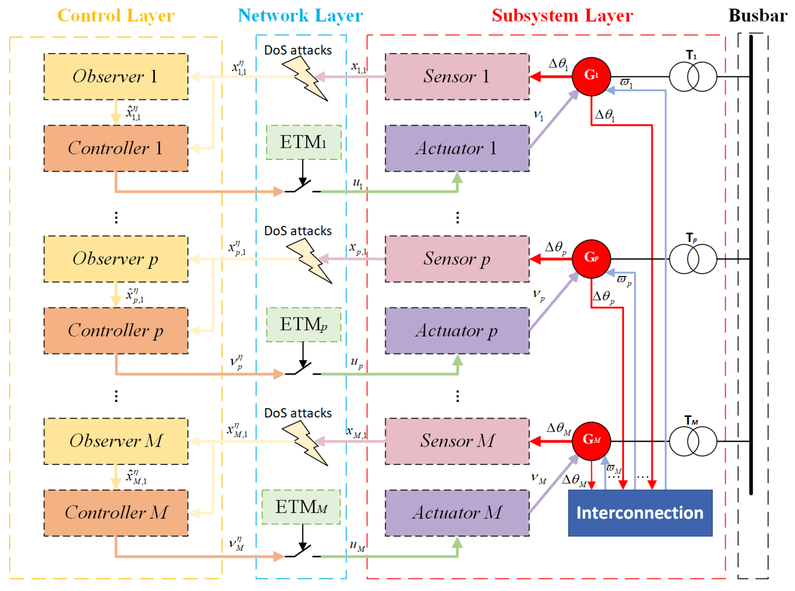
where ${\overline{x}}_p={[x_{p,1},x_{p,2},x_{p,3}]}^T$ represents system state vectors, and $d_p\left(t\right)$ denotes the unmodeled interconnection effect induced by the decentralized separation of the interconnection dynamics. ${\kappa }_p\left({\overline{x}}_p\right)$ represents unknown nonlinear smooth functions. $u_p\in R$ represents the system input and ${\psi }_p={\displaystyle \frac{D_p}{2I_p}}$. And the control framework for the interconnected power system is shown in Figure 1.

Remark 1.

It should be clarified that the physical interconnection among generators may make the exact nonlinear dynamics of the p-th generator depend on the states of other generators. However, under the decentralized control framework and DoS attack environment considered in this paper, the local controller of the p-th generator is designed based on its local estimated state ${\widehat{\overline{x}}}_p$. Therefore, the notation ${\kappa }_p\left({\overline{x}}_p\right)$ in (19) is used as a compact local representation of the unknown dynamics to be compensated by the neural network. ${\mu }_{p,3}^{\ast T}{\mathrm{\Psi }}_{p,3}\left({\widehat{\overline{x}}}_p\right)+{\tau }_{p,3}$, where ${\tau }_{p,3}$ denotes the total approximation error, including the neural network approximation error, the error induced by using estimated states, and the bounded unmodeled interconnection effect. According to Assumption 3 and the boundedness of the neural network basis functions, the total approximation error is bounded, i.e., $|{\tau }_{p,3}|\le {\overline{\tau }}_{p,3}$, where ${\overline{\tau }}_{p,3}$ is an unknown positive constant. Therefore, the local neural network approximation does not require the controller to directly access the states of other generators, and the bounded interconnection effects can be handled through the residual error term used in the subsequent Lyapunov stability analysis.

3.1. Adaptive Switching Neural Network State Observer

Due to the unavailability of system states during DoS attacks, it is necessary to design an adaptive switching neural network state observer that can accurately estimate the system states to mitigate the adverse effects of DoS attacks on the system.

According to Lemma 3 and Remark 2, the unknown nonlinear function ${\kappa }_p\left({\overline{x}}_p\right)$ can be expressed as follows:

$$S_{p,3}({\widehat{\overline{x}}}_p)={\kappa }_p\left({\overline{x}}_p\right)={\mu }_{p,3}^{\ast T}{\mathrm{\Psi }}_{p,3}({\widehat{\overline{x}}}_p)+{\tau }_{p,3}$$

(20)

where ${\widehat{\overline{x}}}_p=[{\widehat{x}}_{p,1},{\widehat{x}}_{p,2},{\widehat{x}}_{p,3}{]}^T$, ${\tau }_{p,3}$ is the total residual error defined in Remark 2, with $|{\tau }_{p,3}|<{\overline{\tau }}_{p,3}$. ${\mathrm{\Psi }}_{p,3}({\widehat{\overline{x}}}_p)$ can be simplified to ${\mathrm{\Psi }}_{p,3}$.

Remark 2.

It is crucial to clarify the treatment of state mismatch between the true state ${\overline{x}}_p$ and the estimated state $\widehat{¯}{x}_p$ in the neural network approximation. To resolve this issue, we first decomposed the nonlinear function as $\kappa ({\overline{x}}_p)=\kappa ({\widehat{\overline{x}}}_p)+{\mathrm{\Delta }}_{p,3}$, where ${\mathrm{\Delta }}_{p,3}={\kappa }_p({\overline{x}}_p)-{\kappa }_p({\widehat{\overline{x}}}_p)$ denotes the state-estimation mismatch term. Since ${\kappa }_p(·)$ is a smooth function, it is locally Lipschitz on the considered compact operating set. Therefore, there exists a positive constant $L_{\kappa p}>0$ such that $|{\mathrm{\Delta }}_{p,3}|\le L_{\kappa p}|{\overline{x}}_p-{\widehat{\overline{x}}}_p|=L_{\kappa p}|{\tilde{\overline{x}}}_p|$. Then the RBFNN is used to approximate ${\kappa }_p({\widehat{\overline{x}}}_p)={\mu }_{p,3}^{\ast T}{\mathrm{\Psi }}_{p,3}({\widehat{\overline{x}}}_p)+{\epsilon }_{p,3}({\widehat{\overline{x}}}_p)$, where ${\epsilon }_{p,3}({\widehat{\overline{x}}}_p)$ denotes the RBFNN approximation error satisfying $|{\epsilon }_{p,3}({\widehat{\overline{x}}}_p)|<{\overline{\epsilon }}_{p,3}$, and the mismatch term is explicitly included in the total residual error. Accordingly, ${\kappa }_p({\overline{x}}_p)={\mu }_{p,3}^{\ast T}{\mathrm{\Psi }}_{p,3}({\widehat{\overline{x}}}_p)+{\tau }_{p,3}$, where ${\tau }_{p,3}={\epsilon }_{p,3}({\widehat{\overline{x}}}_p)+{\mathrm{\Delta }}_{p,3}+d_p$ now denotes the total residual error, including the RBFNN approximation error ${\epsilon }_{p,3}({\widehat{\overline{x}}}_p)$, the state-estimation mismatch error ${\mathrm{\Delta }}_{p,3}$, and the bounded unmodeled interconnection effect $d_p$ mentioned in Assumption 3. Accordingly, the boundedness of ${\tau }_{p,3}$ is rigorously justified and ${\tau }_{p,3}<{\overline{\tau }}_{p,3}$ naturally holds.

According to (19), the state observer is constructed as follows:

$$\left\{\begin{array}{cc}\hfill {\dot{\widehat{x}}}_{p,1}=& {\widehat{x}}_{p,2}+f_{p,1}^{\eta }{\tilde{x}}_{p,1}^{\eta }\hfill \\ \hfill {\dot{\widehat{x}}}_{p,2}=& {\widehat{x}}_{p,3}-{\psi }_p{\widehat{x}}_{p,2}+f_{p,2}^{\eta }{\tilde{x}}_{p,1}^{\eta }\hfill \\ \hfill {\dot{\widehat{x}}}_{p,3}=& u_p+{\widehat{\mu }}_{p,3}^T{\mathrm{\Psi }}_{p,3}+f_{p,3}^{\eta }{\tilde{x}}_{p,1}^{\eta }\hfill \end{array}\right.$$

(21)

where $f_{p,l}^{\eta }(l=1,2,3)$ is a design parameters. $\eta$ represents whether the system is in the state of DoS attack. When $t\in \mathrm{\Lambda }(0,+\infty )$, $\eta =0$ and ${\tilde{x}}_{p,1}^{\eta }=-{\widehat{x}}_{p,1}$. When $t\in \mathrm{\Pi }(0,+\infty )$, $\eta =1$ and ${\tilde{x}}_{p,1}^{\eta }=x_{p,1}-{\widehat{x}}_{p,1}$; ${\tilde{\mu }}_{p,3}^T={\mu }_{p,3}^{\ast T}-{\widehat{\mu }}_{p,3}^T$ denotes the estimation errors. ${\widehat{\mu }}_{p,3}^T$ is the estimation of ${\mu }_{p,3}^{\ast T}$.

Remark 3.

The parameter $f_{p,l}^{\eta }$ is a switching-type parameter. By setting appropriate values for different situations, it allows for greater flexibility in responding to variations in the system under different situations. Additionally, the constructed state observer employs neural networks to approximate nonlinear functions, thereby achieving superior observation performance.

Considering the estimation errors ${\tilde{x}}_{p,l}=x_{p,l}-{\widehat{x}}_{p,l}(l=1,2,3)$, the derivative of the observation errors are obtained as

$$\left\{\begin{array}{cc}\hfill {\dot{\tilde{x}}}_{p,1}=& {\tilde{x}}_{p,2}-f_{p,1}^{\eta }{\tilde{x}}_{p,1}^{\eta }\hfill \\ \hfill {\dot{\tilde{x}}}_{p,2}=& {\tilde{x}}_{p,3}-{\psi }_p{\tilde{x}}_{p,2}-f_{p,2}^{\eta }{\tilde{x}}_{p,1}^{\eta }\hfill \\ \hfill {\dot{\tilde{x}}}_{p,3}=& {\tilde{\mu }}_{p,3}^T{\mathrm{\Psi }}_{p,3}+{\tau }_{p,3}-f_{p,3}^{\eta }{\tilde{x}}_{p,1}^{\eta }\hfill \end{array}\right.$$

(22)

The equality (22) can be rewritten as

$${\dot{\tilde{x}}}_p=A_p{\tilde{x}}_p+{\mathrm{\Psi }}_p^T{\tilde{\mu }}_p+{\tau }_p-f_p^{\eta }{\tilde{x}}_{p,1}^{\eta }$$

(23)

where $A_p=\left[\begin{array}{ccc}0& & \\ ⋮& I^{2\times 2}& \\ 0& \cdots & 0\end{array}\right]$ and $f_p^{\eta }={[f_{p,1}^{\eta },f_{p,2}^{\eta },f_{p,3}^{\eta }]}^T$ is the designed vector, while ${\mathrm{\Psi }}_p=diag\{0,0,{\mathrm{\Psi }}_{p,3}\}$, ${\tau }_p={[0,0,{\tau }_{p,3}]}^T$ and ${\tilde{\mu }}_p={[0,0,{\tilde{\mu }}_{p,3}]}^T$.

Based on the characteristics of the Hurwitz matrix, for any given positive definite matrix $Q_p=Q_p^T>0$, a corresponding positive definite matrix $Z_p^{\eta }=Z_p^{\eta T}>0$ can be found that fulfills

$$A_p^T{Z}_p^{\eta }+Z_p^{\eta }{A}_p=-Q_p^{\eta }$$

(24)

where $Z_p^{\eta }=diag\{Z_{p,1}^{\eta },Z_{p,2}^{\eta },Z_{p,3}^{\eta }\}$.

The Lyapunov function $V_{p,0}^{\eta }$ is chosen as $V_{p,0}^{\eta }={\tilde{x}}_p^T{Z}_p^{\eta }{\tilde{x}}_p$.

Differentiating the Lyapunov function $V_{p,0}^{\eta }$, it can be obtained as

$$\begin{array}{cc}\hfill {\dot{V}}_{p,0}^{\eta }=& {\dot{\tilde{x}}}_p^T{Z}_p^{\eta }{\tilde{x}}_p+{\tilde{x}}_p^T{Z}_p^{\eta }{\dot{\tilde{x}}}_p\hfill \\ \hfill =& {\tilde{x}}_p^T(A_p^T{Z}_p^{\eta }+Z_p^{\eta }{A}_p){\tilde{x}}_p+2{\tilde{x}}_p^T{Z}_p^{\eta }({\mathrm{\Psi }}_p^T{\tilde{\mu }}_p+{\tau }_p-f_p^{\eta }{\tilde{x}}_{p,1}^{\eta })\hfill \end{array}.$$

(25)

For $t\in \mathrm{\Lambda }(0,+\infty )$, according to Lemma 1 and $0<{\mathrm{\Psi }}_{p,3}^T{\mathrm{\Psi }}_{p,3}\le \rho$, the following result can be obtained

$$\begin{array}{cc}\hfill 2{\tilde{x}}_p^T{Z}_p^{\eta }\left({\mathrm{\Psi }}_p^T{\tilde{\mu }}_p+{\tau }_p\right)& \le 2|Z_p^{\eta }||{\tilde{x}}_p||{\mathrm{\Psi }}_{p,3}||{\tilde{\mu }}_{p,3}|+2|Z_p^{\eta }||{\tilde{x}}_p|\left({\overline{\epsilon }}_{p,3}+{\overline{d}}_p+L_{\kappa p}|{\tilde{x}}_p|\right)\hfill \\ \hfill & \le \left(2{|Z_p^{\eta }|}^2+2L_{\kappa p}|Z_p^{\eta }|\right){|{\tilde{x}}_p|}^2+\rho {|{\tilde{\mu }}_{p,3}|}^2+{\left({\overline{\epsilon }}_{p,3}+{\overline{d}}_p\right)}^2\hfill \end{array}$$

(26)

$$2{\tilde{x}}_p^T{Z}_p^0{f}_p^0{\widehat{x}}_{p,1}\le {\Vert {\tilde{x}}_p\Vert }^2{\Vert Z_p^0\Vert }^2+{\Vert f_p^0\Vert }^2{\widehat{x}}_{p,1}^2.$$

(27)

Substituting (24) and (25) into (23) yields

$$\begin{array}{c}\hfill {\dot{V}}_{p,0}^0\le -({\lambda }_{Q_{\min }^0}-3\Vert Z_p^0{\Vert }^2-2L_{\kappa p}\Vert Z_p^0\Vert )\Vert {\tilde{x}}_p{\Vert }^2+\rho \Vert {\tilde{\mu }}_{p,3}{\Vert }^2+{\mathrm{\Theta }}_p^0\end{array}$$

(28)

where ${\lambda }_{Q_{\min }^0}$ is the minimum eigenvalue of the matrix $Q_p^0$, with ${\lambda }_{Q_{\min }^0}-3{\Vert Z_p^0\Vert }^2-2L_{\kappa p}\Vert Z_p^0\Vert >0$ and ${\mathrm{\Theta }}_p^0={\left({\overline{\epsilon }}_{p,3}+{\overline{d}}_p\right)}^2+{\Vert f_p^0\Vert }^2{\widehat{x}}_{p,1}^2$.

For $t\in \mathrm{\Pi }\left(0,+\infty \right)$, similar to Inequality (24), there is

$$2{\tilde{x}}_p^T{Z}_p^1({\mathrm{\Psi }}_p^T{\tilde{\mu }}_p+{\tau }_p)\le \left(2\Vert Z_p^1{\Vert }^2+2L_{\kappa p}\Vert Z_p^1\Vert \right)\Vert {\tilde{x}}_p{\Vert }^2+\rho \Vert {\tilde{\mu }}_{p,3}{\Vert }^2+{\left({\overline{\epsilon }}_{p,3}+{\overline{d}}_p\right)}^2$$

(29)

Substituting (29) into (25) yields

$$\begin{array}{c}\hfill {\dot{V}}_{p,0}^1\le -({\lambda }_{Q_{\min }^1}-2\Vert Z_p^1{\Vert }^2-2L_{\kappa p}\Vert Z_p^1\Vert )\Vert {\tilde{x}}_p{\Vert }^2+\rho \Vert {\tilde{\mu }}_p{\Vert }^2+{\mathrm{\Theta }}_p^1\end{array}$$

(30)

where ${\lambda }_{Q_{\min }^1}$ is the minimum eigenvalue of the matrix $Q_p^1$, while ${\lambda }_{Q_{\min }^1}-2\Vert Z_p^1{\Vert }^2-2L_{\kappa p}\Vert Z_p^1\Vert >0$, $L=[1,0,0]$ and ${\mathrm{\Theta }}_p^1={\left({\overline{\epsilon }}_{p,3}+{\overline{d}}_p\right)}^2$.

3.2. Adaptive Fixed-Time Dynamic Triggered Control Design

In this section, the adaptive fixed-time dynamic triggered control is devised using backstepping technology. Simultaneously, the dynamic surface method is employed to tackle the explosion of a complexity problem. $x_{p,1}^{\eta }$ is defined as the information received by the controller from the sensor. When $\eta =0$, $x_{p,1}^{\eta }={\widehat{x}}_{p,1}$. When $\eta =1$, $x_{p,1}^{\eta }=x_{p,1}$. The corresponding coordinate transformations are constructed as follows:

$$\left\{\begin{array}{cc}\hfill z_{p,1}^{\eta }=& x_{p,1}^{\eta }\hfill \\ \hfill z_{p,l}^{\eta }=& {\widehat{x}}_{p,l}^{\eta }-{\chi }_{p,l}^{\eta }\hfill \\ \hfill e_{p,l}^{\eta }=& {\chi }_{p,l}^{\eta }-a_{p,l-1}^{\eta },l=2,3\hfill \end{array}\right.$$

(31)

where $z_{p,1}^{\eta }$ and $z_{p,l}^{\eta }$ represent the errors’ surfaces, $a_{p,l-1}^{\eta }$ represents the virtual control variable, and ${\chi }_{p,l}^{\eta }$ is the output of the filter. $e_{p,l}^{\eta }$ is the filtering error.

Step 1: The following Lyapunov function $V_{p,1}^{\eta }$ is selected as

$$V_{p,1}^{\eta }=V_{p,0}^{\eta }+{\displaystyle \frac{1}{2}}{\left(z_{p,1}^{\eta }\right)}^2.$$

(32)

From (19), (21), and (31), the derivative of the error variable with respect to time is

$$\left\{\begin{array}{cc}\hfill {\dot{z}}_{p,1}^0=& z_{p,2}^0+a_{p,1}^0+e_{p,2}^0-f_{p,1}^0{\widehat{x}}_{p,1},t\in \mathrm{\Lambda }(0,+\infty )\hfill \\ \hfill {\dot{z}}_{p,1}^1=& z_{p,2}^1+a_{p,1}^1+e_{p,2}^1+{\tilde{x}}_{p,2},t\in \mathrm{\Pi }(0,+\infty )\hfill \end{array}.\right.$$

(33)

Combining (32) and (33), differentiating the Lyapunov function $V_{p,1}^{\eta }$ yields

$$\left\{\begin{array}{cc}\hfill {\dot{V}}_{p,1}^0=& {\dot{V}}_{p,0}^0+z_{p,1}^0{\dot{z}}_{p,1}^0=z_{p,1}^0(z_{p,2}^0+a_{p,1}^0+e_{p,2}^0-f_{p,1}^0{\widehat{x}}_{p,1})\hfill \\ \hfill {\dot{V}}_{p,1}^1=& {\dot{V}}_{p,0}^1+z_{p,1}^1{\dot{z}}_{p,1}^1=z_{p,1}^1(z_{p,2}^1+a_{p,1}^1+e_{p,2}^1+{\tilde{x}}_{p,2})\hfill \end{array}.\right.$$

(34)

According to Lemma 1, there is

$$z_{p,1}^{\eta }{e}_{p,2}^{\eta }\le {\displaystyle \frac{{\left(z_{p,1}^{\eta }\right)}^2}{2}}+{\displaystyle \frac{{\left(e_{p,2}^{\eta }\right)}^2}{2}}.$$

(35)

To ensure the convergence and boundedness of $V_{p,1}^{\eta }$, the virtual control law $a_{p,1}^0$ and $a_{p,1}^1$ are, respectively, defined as follows:

$$a_{p,1}^0=-{\phi }_{p,1}^0{\left(z_{p,1}^0\right)}^{2b-1}-{\psi }_{p,1}^0{\left(z_{p,1}^0\right)}^{2d-1}-{\displaystyle \frac{z_{p,1}^0}{2}}+f_{p,1}^0{\widehat{x}}_{p,1}$$

(36)

$$a_{p,1}^1=-{\phi }_{p,1}^1{\left(z_{p,1}^1\right)}^{2b-1}-{\psi }_{p,1}^1{\left(z_{p,1}^1\right)}^{2d-1}-{\displaystyle \frac{z_{p,1}^1}{2}}-{\tilde{x}}_{p,2}$$

(37)

where ${\phi }_{p,1}^0$, ${\psi }_{p,1}^0$, ${\phi }_{p,1}^1$, and ${\psi }_{p,1}^1$ are positive constants, with $0<b<1$ and $d>1$.

Substituting (35), (36), and (37) into (34), one has

$${\dot{V}}_{p,1}^{\eta }={\dot{V}}_{p,0}^{\eta }-{\phi }_{p,1}^{\eta }{\left(z_{p,1}^{\eta }\right)}^{2b}-{\psi }_{p,1}^{\eta }{\left(z_{p,1}^{\eta }\right)}^{2d}+{\displaystyle \frac{{\left(e_{p,2}^{\eta }\right)}^2}{2}}+z_{p,1}^{\eta }{z}_{p,2}^{\eta }.$$

(38)

Step 2: Similarly, the following Lyapunov function $V_{p,2}^{\eta }$ is selected as

$$V_{p,2}^{\eta }=V_{p,1}^{\eta }+{\displaystyle \frac{1}{2}}{\left(z_{p,2}^{\eta }\right)}^2+{\displaystyle \frac{1}{2}}{\left(e_{p,2}^{\eta }\right)}^2.$$

(39)

From (21) and (31), we obtain

$$\begin{array}{cc}\hfill {\dot{z}}_{p,2}^{\eta }=& {\dot{\widehat{x}}}_{p,2}-{\dot{\chi }}_{p,2}^{\eta }\hfill \\ \hfill =& z_{p,3}^{\eta }+{\chi }_{p,3}^{\eta }-{\psi }_p(z_{p,2}^{\eta }+{\chi }_{p,2}^{\eta })+f_{p,2}^{\eta }{\tilde{x}}_{p,1}^{\eta }-{\dot{\chi }}_{p,2}^{\eta }\hfill \\ \hfill =& z_{p,3}^{\eta }+a_{p,2}^{\eta }+e_{p,3}^{\eta }-{\psi }_p(z_{p,2}^{\eta }+a_{p,1}^{\eta }+e_{p,2}^{\eta })\hfill \\ \hfill & +f_{p,2}^{\eta }{\tilde{x}}_{p,1}^{\eta }-{\dot{\chi }}_{p,2}^{\eta }\hfill \end{array}.$$

(40)

Combining (39) and (40) and differentiating the Lyapunov function yields

$$\begin{array}{cc}\hfill {\dot{V}}_{p,2}^{\eta }=& {\dot{V}}_{p,1}^{\eta }+z_{p,2}^{\eta }(z_{p,3}^{\eta }+a_{p,2}^{\eta }+e_{p,3}^{\eta }-{\psi }_p(z_{p,2}^{\eta }+a_{p,1}^{\eta }\hfill \\ \hfill & +e_{p,2}^{\eta })+f_{p,2}^0{\tilde{x}}_{p,1}^{\eta }-{\dot{\chi }}_{p,2}^{\eta })+e_{p,2}^{\eta }{\dot{e}}_{p,2}^{\eta }\hfill \end{array}.$$

(41)

The first-order filter is constructed as follows:

$${\varsigma }_{p,2}^{\eta }{\dot{\chi }}_{p,2}^{\eta }=-{\left(e_{p,2}^{\eta }\right)}^{2b-1}-{\left(e_{p,2}^{\eta }\right)}^{2d-1}$$

(42)

where ${\chi }_{p,2}^{\eta }\left(0\right)=a_{p,1}^{\eta }\left(0\right)$. ${\varsigma }_{p,2}^{\eta }$ is the design positive parameter.

Equation (42) can be rewritten as

$${\dot{\chi }}_{p,2}^{\eta }=-{\displaystyle \frac{{\left(e_{p,2}^{\eta }\right)}^{2b-1}}{{\varsigma }_{p,2}^{\eta }}}-{\displaystyle \frac{{\left(e_{p,2}^{\eta }\right)}^{2d-1}}{{\varsigma }_{p,2}^{\eta }}}.$$

(43)

Then the derivative of $e_{p,2}^{\eta }$ is obtained as

$${\dot{e}}_{p,2}^{\eta }=-{\displaystyle \frac{{\left(e_{p,2}^{\eta }\right)}^{2b-1}}{{\varsigma }_{p,2}^{\eta }}}-{\displaystyle \frac{{\left(e_{p,2}^{\eta }\right)}^{2d-1}}{{\varsigma }_{p,2}^{\eta }}}+{ƛ}_{p,2}^{\eta }$$

(44)

where ${ƛ}_{p,2}^{\eta }$ is a continuous function, with ${ƛ}_{p,2}^{\eta }={\displaystyle \frac{d{a}_{p,1}^{\eta }}{d{z}_{p,1}^{\eta }}}{\dot{z}}_{p,1}^{\eta }$.

According to Lemma 1, there are

$$z_{p,2}^{\eta }(e_{p,3}^{\eta }-{\psi }_p{e}_{p,2}^{\eta })\le {\displaystyle \frac{({\psi }_p+1){\left(z_{p,2}^{\eta }\right)}^2}{2}}+{\displaystyle \frac{{\left(e_{p,3}^{\eta }\right)}^2}{2}}+{\displaystyle \frac{{\psi }_p{\left(e_{p,2}^{\eta }\right)}^2}{2}},$$

(45)

$$e_{p,2}^{\eta }{ƛ}_{p,2}^{\eta }\le {\displaystyle \frac{{\left(e_{p,2}^{\eta }\right)}^2}{2}}+{\displaystyle \frac{{\left({ƛ}_{p,2}^{\eta }\right)}^2}{2}}.$$

(46)

To ensure the convergence and boundedness of $V_{p,2}^{\eta }$, the virtual control law $a_{p,2}^{\eta }$ is defined as follows:

$$\begin{array}{cc}\hfill a_{p,2}^{\eta }=& -{\phi }_{p,2}^{\eta }{\left(z_{p,2}^{\eta }\right)}^{2b-1}-{\psi }_{p,2}^{\eta }{\left(z_{p,2}^{\eta }\right)}^{2d-1}-f_{p,2}^{\eta }{\tilde{x}}_{p,1}^{\eta }\hfill \\ \hfill & +{\psi }_p{a}_{p,1}^{\eta }+{\dot{\chi }}_{p,2}^{\eta }-z_{p,1}^{\eta }+{\displaystyle \frac{{\psi }_p-1}{2}}{z}_{p,2}^{\eta }\hfill \end{array}$$

(47)

where ${\phi }_{p,2}^{\eta }$ and ${\psi }_{p,2}^{\eta }$ are positive constants.

Substituting (45), (46), and (47) into (41), one has

$$\begin{array}{cc}\hfill {\dot{V}}_{p,2}^{\eta }\le & {\dot{V}}_{p,1}^{\eta }-{\phi }_{p,2}^{\eta }{\left(z_{p,2}^{\eta }\right)}^{2b}-{\psi }_{p,2}^{\eta }{\left(z_{p,2}^{\eta }\right)}^{2d}+z_{p,2}^{\eta }{z}_{p,3}^{\eta }-{\displaystyle \frac{{\left(e_{p,2}^{\eta }\right)}^{2b}}{{\varsigma }_{p,2}^{\eta }}}\hfill \\ \hfill & -{\displaystyle \frac{{\left(e_{p,2}^{\eta }\right)}^{2d}}{{\varsigma }_{p,2}^{\eta }}}+{\displaystyle \frac{({\psi }_p+1){\left(e_{p,2}^{\eta }\right)}^2}{2}}+{\displaystyle \frac{{\left(e_{p,3}^{\eta }\right)}^2}{2}}+{\displaystyle \frac{{\left({ƛ}_{p,2}^{\eta }\right)}^2}{2}}\hfill \\ \hfill \le & {\dot{V}}_{p,0}^{\eta }+{\displaystyle \sum _{j=1}^2}\left(-{\phi }_{p,j}^{\eta }{\left(z_{p,j}^{\eta }\right)}^{2b}-{\psi }_{p,j}^{\eta }{\left(z_{p,j}^{\eta }\right)}^{2d}\right)+z_{p,2}^{\eta }{z}_{p,3}^{\eta }\hfill \\ \hfill & -{\displaystyle \frac{{\left(e_{p,2}^{\eta }\right)}^{2b}}{{\varsigma }_{p,2}^{\eta }}}-{\displaystyle \frac{{\left(e_{p,2}^{\eta }\right)}^{2d}}{{\varsigma }_{p,2}^{\eta }}}+{\displaystyle \frac{({\psi }_p+2){\left(e_{p,2}^{\eta }\right)}^2}{2}}\hfill \\ \hfill & +{\displaystyle \frac{{\left(e_{p,3}^{\eta }\right)}^2}{2}}+{\displaystyle \frac{{\left({ƛ}_{p,2}^{\eta }\right)}^2}{2}}\hfill \end{array}.$$

(48)

Step 3: Considering the communication pressure arising from rapid convergence and the need for effective compensation, the event-triggered control strategy is devised as follows:

$$\left\{\begin{array}{cc}\hfill {\nu }_p^{\eta }\left(t\right)=& -(1+{\varphi }_p^{\eta })\left[a_{p,3}^{\eta }tanh({\displaystyle \frac{z_{p,3}^{\eta }{a}_{p,3}^{\eta }}{{\aleph }_p^{\eta }}})+{\overline{\upsilon }}_p^{\eta }tanh({\displaystyle \frac{z_{p,3}^{\eta }{\overline{\upsilon }}_p^{\eta }}{{\aleph }_p^{\eta }}})\right]\hfill \\ \hfill u_p\left(t\right)=& {\nu }_p^{\eta }\left(t_{p,n}\right),t_{p,n}\le t<t_{p,n+1}\hfill \\ \hfill t_{p,n+1}=& inf\left\{t\in R\left|\left|{\partial }_p^{\eta }\left(t\right)\right|\ge {\varphi }_p^{\eta }tanh\left|{\varpi }_p^{\eta }{u}_p\left(t\right)\right|+{\upsilon }_p^{\eta }\right.\right\}\hfill \\ \hfill {\partial }_p^{\eta }\left(t\right)=& {\nu }_p^{\eta }\left(t\right)-u_p\left(t\right)\hfill \end{array}\right.$$

(49)

where ${\nu }_p^{\eta }\left(t\right)$ is the event-triggered control input. ${\partial }_p^{\eta }\left(t\right)$ represents the relative error, and $t_{p,n}$ and $t_{p,n+1}$ represent the latest trigger time and the next trigger time, respectively. ${\varphi }_p^{\eta }={\alpha }_p^{\eta }{e}^{-{\beta }_p^{\eta }\left|u_p\left(t\right)\right|}$. ${\alpha }_p^{\eta }$${\beta }_p^{\eta }$, ${\aleph }_p^{\eta }$, and ${\upsilon }_p^{\eta }$ are designed positive parameters, with $0<{\alpha }_p^{\eta }+{\upsilon }_p^{\eta }<{\overline{\upsilon }}_p^{\eta }$.

Remark 4. 

${\varphi }_p^{\eta }$ is a dynamic parameter. When the input signal $u_p\left(t\right)$ is relatively large, ${\varphi }_p^{\eta }$ will correspondingly decrease; when the input signal $u_p\left(t\right)$ is relatively small, ${\varphi }_p^{\eta }$ will correspondingly increase, thereby dynamically adjusting the threshold range. The parameter $tanh\left|{\varpi }_p^{\eta }{u}_p\left(t\right)\right|$ is constructed based on the characteristics of the hyperbolic tangent function. When the input signal $u_p\left(t\right)$ is relatively large, $tanh\left|{\varpi }_p^{\eta }{u}_p\left(t\right)\right|$ will correspondingly increase; when the input signal $u_p\left(t\right)$ is relatively small, $tanh\left|{\varpi }_p^{\eta }{u}_p\left(t\right)\right|$ will correspondingly decrease, thereby dynamically adjusting the weight of the threshold. Under the influence of these dual dynamic parameters, a more appropriate triggered threshold is obtained, which reduces the triggered frequency of the controller and conserves communication resources.

From $\left|{\xi }_{p,1}^{\eta }\right|\le 1$, $\left|{\xi }_{p,1}^{\eta }\right|\le 1$ and (49), when $t_{p,n}\le t<t_{p,n+1}$, one has ${\nu }_p^{\eta }=u_p+{\xi }_{p,1}^{\eta }{\alpha }_p^{\eta }+{\xi }_{p,2}^{\eta }{\upsilon }_p^{\eta }$. It can be obtained as

$$u_p\le {\nu }_p^{\eta }+{\overline{\upsilon }}_p^{\eta }.$$

(50)

According to Lemma 8, the following result can be gained

$$z_{p,3}^{\eta }{u}_p\left(t\right)\le z_{p,3}^{\eta }{a}_{p,3}^{\eta }+0.557{\aleph }_p^{\eta }$$

(51)

The Lyapunov function $V_{p,3}^{\eta }$ is selected as

$$V_{p,3}^{\eta }=V_{p,2}^{\eta }+{\displaystyle \frac{1}{2}}{\left(z_{p,3}^{\eta }\right)}^{\eta }+{\displaystyle \frac{1}{2}}{\left(e_{p,3}^{\eta }\right)}^2+{\displaystyle \frac{{\tilde{\mu }}_{p,3}^T{\tilde{\mu }}_{p,3}}{2{\vartheta }_{p,3}^{\eta }}}$$

(52)

where ${\vartheta }_{p,3}^{\eta }$ represents the positive parameters.

From (21) and (31), the time derivative of $z_{p,3}^{\eta }$ is given as

$${\dot{z}}_{p,3}^{\eta }={\dot{\widehat{x}}}_{p,3}^{\eta }-{\dot{\chi }}_{p,3}^{\eta }=u_p+{\widehat{\mu }}_{p,3}^T{\mathrm{\Psi }}_{p,3}+f_{p,3}^{\eta }{\tilde{x}}_{p,1}^{\eta }-{\dot{\chi }}_{p,3}^{\eta }.$$

(53)

Combining (52) and (53) and differentiating the Lyapunov function $V_{p,3}^{\eta }$ yields

$$\begin{array}{c}\hfill {\dot{V}}_{p,3}^{\eta }={\dot{V}}_{p,2}^{\eta }+z_{p,3}^{\eta }(u_p+{\mu }_{p,3}^{\ast T}{\mathrm{\Psi }}_{p,3}-{\tilde{\mu }}_{p,3}^T{\mathrm{\Psi }}_{p,3}+f_{p,3}^{\eta }{\tilde{x}}_{p,1}^{\eta }-{\dot{\chi }}_{p,3}^{\eta })+e_{p,3}^{\eta }{\dot{e}}_{p,3}^{\eta }\end{array}$$

(54)

Similar to (42), the first-order filter is constructed as follows:

$${\varsigma }_{p,3}^{\eta }{\dot{\chi }}_{p,3}^{\eta }=-{\left(e_{p,3}^{\eta }\right)}^{2b-1}-{\left(e_{p,3}^{\eta }\right)}^{2d-1}$$

(55)

where ${\chi }_{p,3}^{\eta }\left(0\right)=a_{p,2}^{\eta }\left(0\right)$. ${\varsigma }_{p,3}^{\eta }$ is the design positive parameter.

Equation (55) can be rewritten as

$${\dot{\chi }}_{p,3}^{\eta }=-{\displaystyle \frac{{\left(e_{p,3}^{\eta }\right)}^{2b-1}}{{\varsigma }_{p,3}^{\eta }}}-{\displaystyle \frac{{\left(e_{p,3}^{\eta }\right)}^{2d-1}}{{\varsigma }_{p,3}^{\eta }}}.$$

(56)

Then the derivative of $e_{p,3}^{\eta }$ is obtained as

$${\dot{e}}_{p,3}^{\eta }=-{\displaystyle \frac{{\left(e_{p,3}^{\eta }\right)}^{2b-1}}{{\varsigma }_{p,3}^{\eta }}}-{\displaystyle \frac{{\left(e_{p,3}^{\eta }\right)}^{2d-1}}{{\varsigma }_{p,3}^{\eta }}}+{ƛ}_{p,3}^{\eta }$$

(57)

where ${ƛ}_{p,3}^{\eta }$ is a continuous function, with ${ƛ}_{p,3}^{\eta }={\displaystyle \frac{d{a}_{p,2}^{\eta }}{d{z}_{p,2}^{\eta }}}{\dot{z}}_{p,2}^{\eta }$.

According to Lemma 1, there are

$$-z_{p,3}^{\eta }{\tilde{\mu }}_{p,3}^T{\mathrm{\Psi }}_{p,3}\le {\displaystyle \frac{{\left(z_{p,3}^{\eta }\right)}^2}{2}}+{\displaystyle \frac{\rho \Vert {\tilde{\mu }}_{p,3}{\Vert }^2}{2}},$$

(58)

$$e_{p,3}^{\eta }{ƛ}_{p,3}^{\eta }\le {\displaystyle \frac{{\left(e_{p,3}^{\eta }\right)}^2}{2}}+{\displaystyle \frac{{\left({ƛ}_{p,3}^{\eta }\right)}^2}{2}}.$$

(59)

To ensure the convergence and boundedness of $V_{p,3}^{\eta }$, the virtual control law $a_{p,3}^{\eta }$ and adaptive law ${\dot{\widehat{\mu }}}_{p,3}$ are defined as follows:

$$\begin{array}{cc}\hfill a_{p,3}^{\eta }=& -{\phi }_{p,3}^{\eta }{\left(z_{p,3}^{\eta }\right)}^{2b-1}-{\psi }_{p,3}^{\eta }{\left(z_{p,3}^{\eta }\right)}^{2d-1}-f_{p,3}^{\eta }{\tilde{x}}_{p,1}^{\eta }\hfill \\ \hfill & -{\widehat{\mu }}_{p,3}^T{\mathrm{\Psi }}_{p,3}+{\dot{\chi }}_{p,3}^{\eta }-z_{p,2}^{\eta }-{\displaystyle \frac{z_{p,3}^{\eta }}{2}},\hfill \end{array}$$

(60)

$${\dot{\widehat{\mu }}}_{p,3}=-{\zeta }_{p,3}^{\eta }{\widehat{\mu }}_{p,3}+{\vartheta }_{p,3}^{\eta }{z}_{p,3}^{\eta }{\mathrm{\Psi }}_{p,m}$$

(61)

where ${\phi }_{p,3}^{\eta }$, ${\psi }_{p,3}^{\eta }$ and ${\zeta }_{p,3}^{\eta }$ are positive constants.

Substituting (58), (59), (60), and (61) into (54), one has

$$\begin{array}{cc}\hfill {\dot{V}}_{p,3}^{\eta }\le & {\dot{V}}_{p,2}^{\eta }-{\phi }_{p,3}^{\eta }{z}_{p,3}^{2b}-{\psi }_{p,3}^{\eta }{z}_{p,3}^{2d}+{\displaystyle \frac{{\zeta }_{p,3}^{\eta }{\tilde{\mu }}_{p,3}^T{\widehat{\mu }}_{p,3}}{{\vartheta }_{p,3}^{\eta }}}-{\displaystyle \frac{{\left(e_{p,3}^{\eta }\right)}^{2b}}{{\varsigma }_{p,3}^{\eta }}}\hfill \\ \hfill & -{\displaystyle \frac{{\left(e_{p,3}^{\eta }\right)}^{2d}}{{\varsigma }_{p,3}^{\eta }}}+{\displaystyle \frac{\rho \Vert {\tilde{\mu }}_{p,3}{\Vert }^2}{2}}+{\displaystyle \frac{{\left(e_{p,3}^{\eta }\right)}^2}{2}}+{\displaystyle \frac{{\left({ƛ}_{p,3}^{\eta }\right)}^2}{2}}+0.557{\aleph }_p^{\eta }\hfill \\ \hfill \le & {\dot{V}}_{p,0}^{\eta }-{\displaystyle \sum _{j=1}^3}\left({\phi }_{p,j}^{\eta }{\left(z_{p,j}^{\eta }\right)}^{2b}+{\psi }_{p,j}^{\eta }{\left(z\right)}_{p,j}^{\eta }\right)-{\displaystyle \sum _{j=2}^3}{\displaystyle \frac{{\left(e_{p,j}^{\eta }\right)}^{2b}}{{\varsigma }_{p,j}^{\eta }}}\hfill \\ \hfill & -{\displaystyle \sum _{j=2}^3}{\displaystyle \frac{{\left(e_{p,j}^{\eta }\right)}^{2d}}{{\varsigma }_{p,j}^{\eta }}}+{\displaystyle \frac{{\zeta }_{p,3}^{\eta }{\tilde{\mu }}_{p,3}^T{\widehat{\mu }}_{p,3}}{{\vartheta }_{p,3}^{\eta }}}+{\displaystyle \frac{\rho \Vert {\tilde{\mu }}_{p,3}{\Vert }^2}{2}}\hfill \\ \hfill & +{\displaystyle \sum _{j=2}^3}{\displaystyle \frac{{\left({ƛ}_{p,j}^{\eta }\right)}^2}{2}}+{\displaystyle \frac{({\psi }_p+2){\left(e_{p,2}^{\eta }\right)}^2}{2}}+{\left(e_{p,3}^{\eta }\right)}^2+0.557{\aleph }_p^{\eta }\hfill \end{array}$$

(62)

According to Lemma 1, there is

$${\tilde{\mu }}_{p,3}^T{\widehat{\mu }}_{p,3}={\displaystyle \frac{{\mu }_{p,3}^T{\mu }_{p,3}}{2}}-{\displaystyle \frac{{\tilde{\mu }}_{p,3}^T{\tilde{\mu }}_{p,3}}{2}}.$$

(63)

According to Lemma 6, there is

$$-{\displaystyle \frac{{\tilde{\mu }}_{p,3}^T{\tilde{\mu }}_{p,3}}{{\vartheta }_{p,3}^{\eta }}}\le -{\left({\displaystyle \frac{{\tilde{\mu }}_{p,3}^T{\tilde{\mu }}_{p,3}}{2{\vartheta }_{p,3}^{\eta }}}\right)}^b-{\left({\displaystyle \frac{{\tilde{\mu }}_{p,3}^T{\tilde{\mu }}_{p,3}}{2{\vartheta }_{p,3}^{\eta }}}\right)}^d+{\Im }_p^{\eta }.$$

(64)

According to Lemma 2, letting $l_1=b$, $l_2=1-b$, $\stackrel{⌢}{k}=b^{{\displaystyle \frac{b}{1-b}}}$, ${\stackrel{⌢}{h}}_1=1$, and ${\stackrel{⌢}{h}}_2={\tilde{x}}_p^T{Z}_p^{\eta }{\tilde{x}}_p$, there is

$${\left({\tilde{x}}_p^T{Z}_p^{\eta }{\tilde{x}}_p\right)}^b\le \left(1-b\right)b^{{\displaystyle \frac{b}{1-b}}}+{\tilde{x}}_p^T{Z}_p^{\eta }{\tilde{x}}_p.$$

(65)

Similarly, letting $l_1=d$, $l_2=1-d$, $\stackrel{⌢}{k}=d^{{\displaystyle \frac{d}{1-d}}}$, ${\stackrel{⌢}{h}}_1=1$, and ${\stackrel{⌢}{h}}_2={\tilde{x}}_p^T{Z}_p^{\eta }{\tilde{x}}_p$, there is

$${\left({\tilde{x}}_p^T{Z}_p^{\eta }{\tilde{x}}_p\right)}^d\le \left(1-d\right)d^{{\displaystyle \frac{d}{1-d}}}+{\tilde{x}}_p^T{Z}_p^{\eta }{\tilde{x}}_p.$$

(66)

Combining (28), (30), (63), (64), (65), (66), and Lemma 5, Inequality (62) can be rewritten as follows:

$$\begin{array}{cc}\hfill {\dot{V}}_{p,3}^{\eta }\le & -{\lambda }_{\tilde{x}}^{\eta }\left[{\left({\tilde{x}}_p^T{Z}_p^{\eta }{\tilde{x}}_p\right)}^b+{\left({\tilde{x}}_p^T{Z}_p^{\eta }{\tilde{x}}_p\right)}^d\right]-2^b{\phi }_{\min }^{\eta }{\left({\displaystyle \sum _{j=1}^m}{\displaystyle \frac{z_{\mathrm{\Lambda }p,j}^2}{2}}\right)}^b\hfill \\ & -3^{1-d}{2}^d{\psi }_{\min }^{\eta }{\left({\displaystyle \sum _{j=1}^3}{\displaystyle \frac{z_{\mathrm{\Lambda }p,j}^2}{2}}\right)}^d-{\stackrel{⌢}{\zeta }}_{p,3}^{\eta }{\left({\displaystyle \frac{{\tilde{\mu }}_{p,3}^T{\tilde{\mu }}_{p,3}}{2{\vartheta }_{\mathrm{\Lambda }p,3}}}\right)}^b-{\stackrel{⌢}{\zeta }}_{p,3}^{\eta }{\left({\displaystyle \frac{{\tilde{\mu }}_{p,3}^T{\tilde{\mu }}_{p,3}}{2{\vartheta }_{\mathrm{\Lambda }p,3}}}\right)}^d\hfill \\ & -{\stackrel{⌢}{\varsigma }}_{\min }^{\eta }{\left({\displaystyle \sum _{j=2}^3}{\displaystyle \frac{e_{p,j}^2}{2}}\right)}^b-{\stackrel{⌣}{\varsigma }}_{\min }^{\eta }{\left({\displaystyle \sum _{j=2}^3}{\displaystyle \frac{e_{p,j}^2}{2}}\right)}^d+{\displaystyle \frac{{\zeta }_{p,3}^{\eta }{\mu }_{p,3}^T{\mu }_{p,3}}{2{\vartheta }_{p,3}^{\eta }}}+{\displaystyle \frac{3\rho \Vert {\tilde{\mu }}_{p,3}{\Vert }^2}{2}}\hfill \\ & +{\displaystyle \frac{({\psi }_p+2){\left(e_{p,2}^{\eta }\right)}^2}{2}}+{\displaystyle \sum _{j=2}^3}{\displaystyle \frac{{\left({ƛ}_{p,j}^{\eta }\right)}^2}{2}}+{\lambda }_{\tilde{x}}^{\eta }[(1-b)b^{{\displaystyle \frac{b}{1-b}}}+(1-d)d^{{\displaystyle \frac{d}{1-d}}}]\hfill \\ & +{\left(e_{p,3}^{\eta }\right)}^2+0.557{\aleph }_p^{\eta }+{\stackrel{⌢}{\zeta }}_{p,3}^{\eta }{\Im }_p^{\eta }+{\mathrm{\Theta }}_p^{\eta }\hfill \end{array}$$

(67)

where ${\lambda }_{Z_{max}^{\eta }}$ is the maximum eigenvalue of the matrix $Z_p^{\eta }$. When $\eta =0$, ${\lambda }_{\tilde{x}}^0={\displaystyle \frac{\left({\lambda }_{Q_{\min }^0}-3\Vert Z_p^0{\Vert }^2-2L_{\kappa p}\Vert Z_p^0\Vert \right)}{2{\lambda }_{Z_{max}^0}}}$. When $\eta =1$, ${\lambda }_{\tilde{x}}^1={\displaystyle \frac{\left({\lambda }_{Q_{\min }^1}-2\Vert Z_p^1{\Vert }^2-2L_{\kappa p}\Vert Z_p^1\Vert \right)}{2{\lambda }_{Z_{max}^1}}}$; ${\phi }_{\min }^{\eta }=\min [{\phi }_{p,1}^{\eta },{\phi }_{p,2}^{\eta },{\phi }_{p,3}^{\eta }]$, ${\psi }_{\min }^{\eta }=\min [{\psi }_{p,1}^{\eta },{\psi }_{p,2}^{\eta },{\psi }_{p,3}^{\eta }]$, ${\stackrel{⌢}{\zeta }}_{p,3}^{\eta }={\displaystyle \frac{{\zeta }_{p,3}^{\eta }}{2}}-{\displaystyle \frac{3\rho {\vartheta }_{p,3}^{\eta }}{2}}$, ${\stackrel{⌢}{\varsigma }}_{\min }^{\eta }=\min [2^b/{\varsigma }_{p,2}^{\eta },2^b/{\varsigma }_{p,3}^{\eta }]$, and ${\stackrel{⌣}{\varsigma }}_{\min }^{\eta }=\min [2^d/{\varsigma }_{p,2}^{\eta },2^d/{\varsigma }_{p,3}^{\eta }]$.

From Lemma 7, Inequality (67) can be transformed as follows:

$${\dot{V}}_{p,3}^{\eta }\le -{\hslash }_{\mathrm{p}1}^{\eta }{\left(V_{p,3}^{\eta }\right)}^b-{\hslash }_{\mathrm{p}2}^{\eta }{\left(V_{p,3}^{\eta }\right)}^d+{\mathrm{{\rm Y}}}_p^{\eta }$$

(68)

where ${\hslash }_{p1}^{\eta }=\min [{\lambda }_{\tilde{x}}^{\eta },2^b{\phi }_{\min }^{\eta },{\stackrel{⌢}{\zeta }}_{p,3}^{\eta },{\stackrel{⌢}{\varsigma }}_{\min }^{\eta }]$, ${\hslash }_{p2}^{\eta }=\min [{\lambda }_{\tilde{x}}^{\eta },3^{1-d}{2}^d{\psi }_{\min }^{\eta },{\stackrel{⌢}{\zeta }}_{p,3}^{\eta },\stackrel{⌣}{\varsigma }]$, and ${\mathrm{{\rm Y}}}_p^{\eta }={\displaystyle \frac{{\zeta }_{p,3}^{\eta }{\mu }_{p,3}^T{\mu }_{p,3}}{2{\vartheta }_{p,3}^{\eta }}}+{\displaystyle \frac{3\rho \Vert {\tilde{\mu }}_{p,3}{\Vert }^2}{2}}+{\displaystyle \frac{({\psi }_p+2){\left(e_{p,2}^{\eta }\right)}^2}{2}}+{\displaystyle \sum _{j=2}^3}{\displaystyle \frac{({\mathrm{ƛ}}_{p,j}^{\eta }{)}^2}{2}}+{\lambda }_{\tilde{x}}^{\eta }[(1-b)b^{{\displaystyle \frac{b}{1-b}}}+(1-d)d^{{\displaystyle \frac{d}{1-d}}}]+{\left(e_{p,3}^{\eta }\right)}^2+0.557{\aleph }_p^{\eta }+{\stackrel{⌢}{\zeta }}_{p,3}^{\eta }{\Im }_p^{\eta }+{\mathrm{\Theta }}_p^{\eta }$.

3.3. System Analysis

Theorem 1.

For a class of interconnected power system (1), state observer (21), model (19) after system transformation, virtual control laws (36), (37), (47), and (60), adaptive law (22), an ETM (49), the stated objectives are guaranteed as follows:

(1) 

The proposed state observer and controller can guarantee that the closed-loop signals of systems are bounded under DoS attacks.

(2) 

The controlled system achieves practical fixed-time convergence within a fixed time interval, and the convergence performance of the systems subject to DoS attacks can be guaranteed.

(3) 

The Zeno behavior can be effectively eliminated.

Proof. 

From (68), when ${\left(V_{p,3}^{\eta }\right)}^d\ge ({\mathrm{{\rm Y}}}_p^{\eta }/{\hslash }_{p2}^{\eta })$, according to the Lyapunov stability theorem, $V_{p,3}^{\eta }$ is bounded, i.e., the error signals $z_{p,l}^{\eta }(l=1,2,3)$, ${\tilde{x}}_{p,l}^{\eta }$, $e_{p,2}^{\eta }$, $e_{p,3}^{\eta }$, and ${\tilde{\mu }}_{p,3}$ are bounded. Thus, it can be obtained that $x_{p,l}$, ${\widehat{x}}_{p,l}$, $a_{p,l}^{\eta }$, ${\widehat{\mu }}_{p,3}$, and ${\chi }_{p,2}^{\eta }$ are also bounded.

When ${\left(V_{p,3}^{\eta }\right)}^d<({\mathrm{{\rm Y}}}_p^{\eta }/{\hslash }_{p2}^{\eta })$, (68) can be rewritten as

$${\dot{V}}_{p,3}^{\eta }\le -{\hslash }_{p1}^{\eta }{\left(V_{p,3}^{\eta }\right)}^b+K$$

(69)

where $K\le 0$, and, according to Lemma 4, it can be known that in this situation the system is also stable. Then, all the signals are bounded.

From the above analysis, it can be concluded that the boundedness of all signals is guaranteed.

According to Lemma 7 and Inequality (68), the error signal ${\mathrm{\Xi }}_p$ converges to the following set

$$\begin{array}{c}\hfill {\mathrm{\Delta }}_p=\{{\mathrm{\Xi }}_p|V_{p,3}^{\eta }\left({\mathrm{\Xi }}_p\right)\le \min \{{({\displaystyle \frac{{\mathrm{{\rm Y}}}_p}{{\hslash }_{p1}\left(1-{\beta }_p\right)}})}^{{\displaystyle \frac{1}{b}}},\\ \hfill {({\displaystyle \frac{{\mathrm{{\rm Y}}}_p}{{\hslash }_{p2}\left(1-{\beta }_p\right)}})}^{{\displaystyle \frac{1}{d}}}\left\}\right\}\end{array}.$$

(70)

where ${\mathrm{\Xi }}_p={[z_{p,1}^{\eta },z_{p,2}^{\eta },z_{p,3}^{\eta },{\tilde{x}}_{p,1}^{\eta },{\tilde{x}}_{p,2}^{\eta },{\tilde{x}}_{p,3}^{\eta },e_{p,2}^{\eta },e_{p,3}^{\eta },{\tilde{\mu }}_{p,3}]}^T$.

The convergence time $T_p$ is as follows:

$$T_p\le {\displaystyle \frac{1}{{\hslash }_{p1}{\beta }_p\left(1-b\right)}}+{\displaystyle \frac{1}{{\hslash }_{p2}{\beta }_p\left(d-1\right)}}.$$

(71)

Thus, the error signal ${\mathrm{\Xi }}_p$ converges within a fixed time $T_p$ to a bounded range ${\mathrm{\Delta }}_p$, indicating that $x_{p,1},\cdots ,x_{p,3},{\widehat{x}}_{p,1},\cdots ,{\widehat{x}}_{p,3},a_{p,1}^{\eta },\cdots ,a_{p,3}^{\eta },{\widehat{\mu }}_{p,3},{\chi }_{p,2}^{\eta },{\chi }_{p,3}^{\eta }$ are bounded.

Remark 5.

The system can achieve rapid convergence by selecting the appropriate parameters. And the upper bound of the convergence time $T_p$ is independent of the initial state.

Based on the definition of $V_{p,3}^{\eta }$ and (70), it can be deduced that

$$|{\mathrm{z}}_{p,l}|\le \min \left\{\sqrt{2}{({\displaystyle \frac{{\mathrm{{\rm Y}}}_p}{{\hslash }_{p2}(1-{\beta }_p)}})}^{{\displaystyle \frac{1}{2b}}},\sqrt{2}{({\displaystyle \frac{{\mathrm{{\rm Y}}}_p}{{\hslash }_{p1}(1-{\beta }_p)}})}^{{\displaystyle \frac{1}{2d}}}\right\}.$$

(72)

Thus, the error surface ${\mathrm{z}}_{p,l}(l=1,2,3)$ can converge to a small and adjustable set within a fixed time, ensuring the practical fixed-time convergence of the system.

According to the event-triggered strategy (49), the control input $u_p\left(t\right)$ remains constant, and thus

$${\dot{\partial }}_p^{\eta }\left(t\right)={\dot{\nu }}_p^{\eta }\left(t\right).$$

(73)

Meanwhile, the implemented control input $u_p\left(t\right)={\nu }_p^{\eta }\left(t_{p,n}\right)$ remains constant. Hence, the dynamic parameter ${\varphi }_p^{\eta }={\alpha }_p^{\eta }{e}^{-{\beta }_p^{\eta }|u_p\left(t\right)|}$ is also constant over this interval, which gives ${\dot{\varphi }}_p^{\eta }\left(t\right)=0$.

From the preceding Lyapunov analysis, all closed-loop signals are bounded. Moreover, from the system dynamics, observer dynamics, adaptive laws, and nonlinear filters, the signals entering the virtual control law ${\alpha }_{p,3}^{\eta }$ and the error surface $z_{p,3}^{\eta }$ are composed of bounded signals and smooth mappings on the considered compact set. Under the designed parameter conditions, their time derivatives are also bounded. Therefore, one obtains $|z_{p,3}^{\eta }|\le {\overline{z}}_{p,3},|a_{p,3}^{\eta }|\le {\overline{a}}_{p,3},|{\dot{z}}_{p,3}^{\eta }|\le {\overline{\dot{}}z}_{p,3},|{\dot{a}}_{p,3}^{\eta }|\le {\overline{\dot{}}a}_{p,3}$

Using $|tanh(·)|\le 1$ and $0<{\mathrm{sech}}^2(·)\le 1$, the derivation of ${\nu }_p^{\eta }\left(t\right)$ satisfies

$$|{\dot{\nu }}_p^{\eta }\left(t\right)|\le (1+{\alpha }_p^{\eta })[{\overline{\dot{}}a}_{p,3}+{\displaystyle \frac{{\overline{a}}_{p,3}}{{\aleph }_p^{\eta }}}\left({\overline{\dot{}}z}_{p,3}{\overline{a}}_{p,3}+{\overline{z}}_{p,3}{\overline{\dot{}}a}_{p,3}\right)+{\displaystyle \frac{{\left({\overline{\upsilon }}_p^{\eta }\right)}^2}{{\aleph }_p^{\eta }}}{\overline{\dot{}}z}_{p,3}]={\overline{\nu }}_p^{\eta }$$

(74)

Therefore, ${\dot{\nu }}_p^{\eta }\left(t\right)$ is uniformly bounded on each inter-event interval.

Then, the derivative of $|{\partial }_p^{\eta }\left(t\right)|$ satisfies

$${\displaystyle \frac{d|{\partial }_p^{\eta }\left(t\right)|}{dt}}=\mathrm{sgn}\left({\nu }_p^{\eta }\right){\dot{\nu }}_p^{\eta }\le {\overline{\nu }}_p^{\eta }$$

(75)

Since ${\partial }_p^{\eta }\left(t_{p,n}\right)=0$, integrating (75) over $\left[t_{p,n},t\right]$ gives

$$|{\partial }_p^{\eta }\left(t\right)|\le \overline{\nu }{p}^{\eta }(t-t_{p,n})$$

(76)

At the next triggering instant $t_{p,n+1}$, the triggering condition (49) is satisfied, namely,

$$|{\partial }_p^{\eta }(t_{p,n+1})|\ge {\varphi }_p^{\eta }tanh\left(|{\varpi }_p^{\eta }{u}_p\left(t\right)|\right)+{\upsilon }_p^{\eta }$$

(77)

therefore, the inter-event interval satisfies

$$t_{p,n+1}-t_{p,n}\ge {\displaystyle \frac{{\varphi }_p^{\eta }tanh\left(|{\varpi }_p^{\eta }{u}_p\left(t\right)|\right)+{\upsilon }_p^{\eta }}{{\overline{\nu }}_p^{\eta }}}$$

(78)

Since ${\varphi }_p^{\eta }>0$, ${\upsilon }_p^{\eta }>0$, and ${\overline{\nu }}_p^{\eta }>0$, there exists a positive constant

$$t^{\ast }={\displaystyle \frac{{\varphi }_p^{\eta }tanh\left(|{\varpi }_p^{\eta }{u}_p\left(t\right)|\right)+{\upsilon }_p^{\eta }}{{\overline{\nu }}_p^{\eta }}}>0$$

(79)

such that

$$t_{p,n+1}-t_{p,n}\ge t^{\ast }>0$$

(80)

Hence, the inter-event time is strictly lower bounded by a positive constant, which implies that infinite triggering cannot occur within a finite time interval. Therefore, Zeno behavior is effectively excluded. □

4. Simulation Results

4.1. Simulation Setup and Analysis

In this section, numerical simulations are carried out to verify the effectiveness of the proposed adaptive practical fixed-time dynamic triggered control method for interconnected power systems under DoS attacks. A two-generator interconnected synchronous generator system is considered as the simulation object. The main objectives of this section are to validate the state convergence performance under DoS attacks, the effectiveness of the proposed adaptive switching neural network state observer, and the communication-saving capability of the proposed dynamic ETM. The physical parameters of the interconnected power system are listed in

Table 2. System parameters.

Parameter	Value	Parameter	Value	Parameter	Value	Parameter	Value
$D_1$	$1\mathrm{N}·\mathrm{s}/\mathrm{m}$	$D_2$	$1\mathrm{N}·\mathrm{s}/\mathrm{m}$	$I_1$	$6.35\mathrm{s}$	$I_2$	$6.4\mathrm{s}$
$T_1$	$6\mathrm{s}$	$T_2$	$6\mathrm{s}$	$E_1$	$0.2$	$E_2$	$0.05$
$B_{12}$	$9.3\times {10}^{-5}$	$B_{21}$	$2.493\times {10}^{-3}$	$G_{12}$	$4.1\times {10}^{-5}$	$G_{21}$	$3.41\times {10}^{-4}$
${\theta }_{0,1}$	$1\mathrm{rad}$	${\theta }_{0,2}$	$1.2\mathrm{rad}$	${\omega }_0$	$314.159\mathrm{rad}/\mathrm{s}$

.

The initial states of the system are given as follows: $x_{p,1}=[0.5,0.5]$, $x_{p,1}=[0.4,0.4]$, $x_{p,3}={[0.3,0.3]}^T$, and $p=1,2$.

Then, the control parameters are selected as follows: $b={\displaystyle \frac{4}{5}}$, $d=2$, $f_p^0={[3,5,3]}^T$, $f_p^1={[0.2,0.2,0.2]}^T$, ${\varsigma }_{1,2}^{\eta }=0.24$, ${\varsigma }_{1,3}^{\eta }=0.1$, ${\varphi }_{1,1}=0.2$, ${\varphi }_{1,2}^{\eta }=1$, ${\varphi }_{1,3}^{\eta }=12$, ${\psi }_{1,1}^{\eta }=0.5$, ${\psi }_{1,2}^{\eta }=0.2$, ${\psi }_{1,3}^{\eta }=0.5$, ${\zeta }_{1,3}^{\eta }=0.5$, ${\vartheta }_{1,3}^{\eta }=0.5$, ${\varsigma }_{2,2}^{\eta }=0.24$, ${\varsigma }_{2,3}^{\eta }=0.1$, ${\varphi }_{2,1}^{\eta }=0.3$, ${\varphi }_{2,2}^{\eta }=1$, ${\varphi }_{2,3}^{\eta }=10$, ${\psi }_{2,l}^{\eta }=0.3$, ${\psi }_{2,2}^{\eta }=0.1$, ${\psi }_{2,3}^{\eta }=0.5$, and ${\zeta }_{2,3}^{\eta }=0.5$, ${\vartheta }_{2,3}^{\eta }=0.5$.

The parameters for the control strategy triggered by events are designed as follows: ${\alpha }_p^{\eta }=0.7$, ${\beta }_p^{\eta }=0.6$, ${\varpi }_p^{\eta }=2$, ${\upsilon }_p^{\eta }=0.1$, and ${\aleph }_p^{\eta }=0.4$.

Remark 6.

The adaptive parameters and control gains introduced in the proposed method are controller design parameters rather than direct physical parameters of the power system. These parameters are selected according to the theoretical requirements in the stability analysis and then adjusted empirically through simulations. In general, the convergence-related parameters are tuned by considering their influence on practical fixed-time convergence performance, where larger control gains usually lead to faster convergence but may also increase the control input amplitude. The observer and adaptive parameters are chosen to ensure satisfactory state estimation and compensation performance. Meanwhile, the event-triggered parameters are adjusted to achieve a trade-off between control accuracy and communication resource saving. Therefore, the final parameter set is determined by jointly considering convergence speed, control smoothness, estimation performance, and triggering frequency.

The simulation results are illustrated as follows:

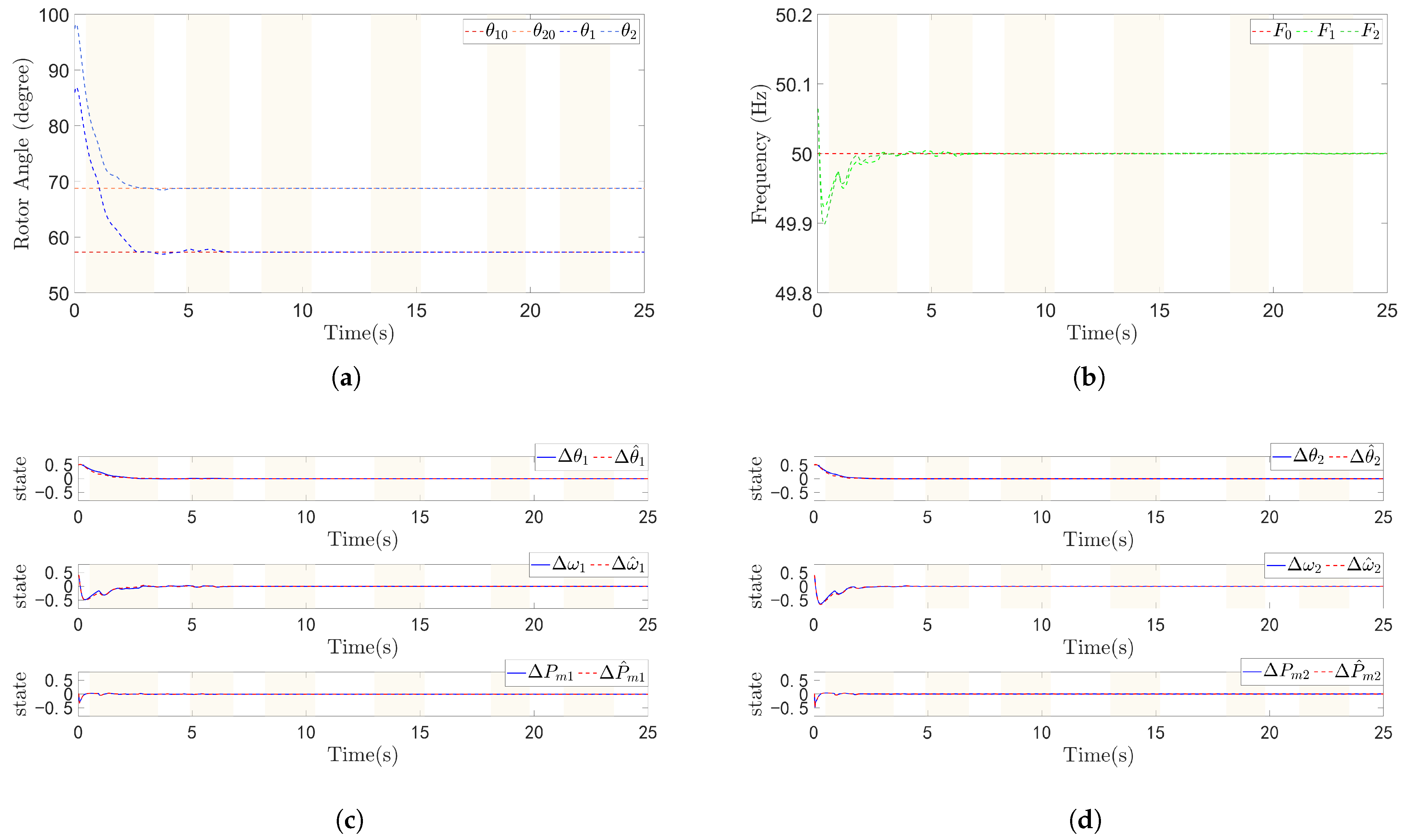
As shown in Figure 2, It can be observed that when the system is subjected to DoS attacks during the convergence process in the interval $t\in \left[0.5,3.5\right]$, the convergence of the synchronous generators is affected, but the system can still converge rapidly. Furthermore, when the system is subjected to DoS attacks after convergence in the interval $t\in \left[13,15\right]$, the system can still maintain convergence within a small range without becoming unstable. Obviously, irrespective of the presence or timing of DoS attacks, the proposed control method enables the rotor angle and frequency of the generators to rapidly track the nominal values. And all system state deviations can converge within a fixed time and remain within a small range, therefore confirming the effectiveness of the control method.

It can be further observed from Figure 2 that the simulation results are consistent with the design purpose of the proposed controller and observer. Figure 2a,b verify the convergence performance of the closed-loop system under DoS attacks, which supports the practical fixed-time control capability of the proposed method. Meanwhile, Figure 2c,d show that the proposed adaptive switching neural network state observer can provide effective state estimation for both generators. This indicates that the observer can compensate for the unavailable sensor information during DoS attacks and provide the required estimated states for the controller. Therefore, Figure 2 directly supports the effectiveness of the observer-based compensation and practical fixed-time control design proposed in this work.

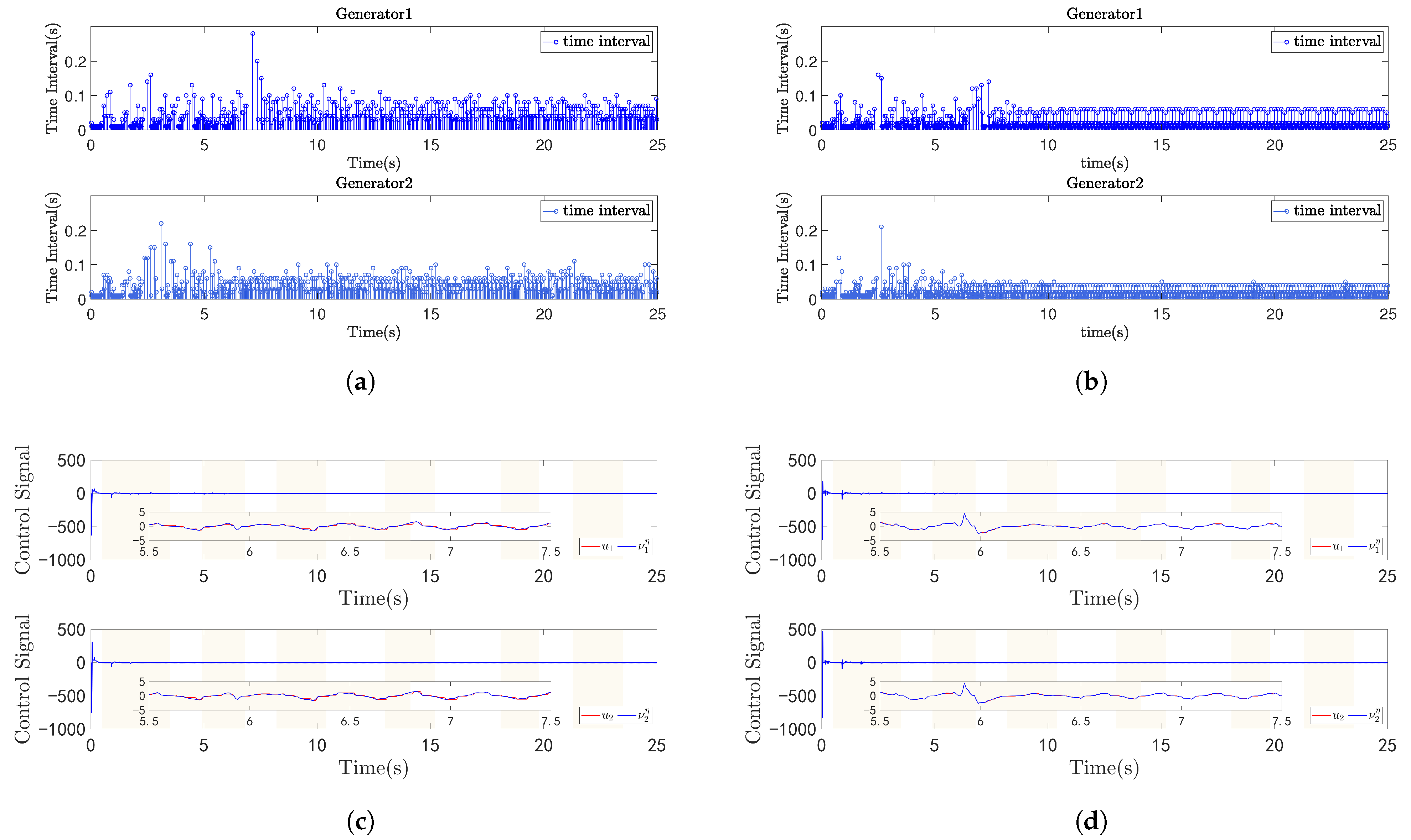
The comparison of different triggering mechanisms is presented in Figure 3. The compared ETM is adopted from [34]. Figure 3a,b shows the triggered intervals of the proposed method and the compared method, respectively. From these two subfigures, it can be observed that the proposed method generates sparser triggering instants and longer triggering intervals than the compared method under the same simulation setting. Meanwhile, the minimum triggered interval is 0.01 s. The control input $u_p$ and the event-triggered signal ${\nu }_p^{\eta }$ of the proposed method and the compared method are shown in Figure 3c,d, respectively. These results indicate that the proposed method can maintain effective control performance while reducing unnecessary control updates. The quantitative comparison of different triggering mechanisms is further listed in

Table 3. Number of triggered events under different triggering mechanisms.

Triggering Mechanism	Generator 1	Generator 2
Time-triggered mechanism	2500	2500
Compared event-triggered mechanism	1225	1214
Proposed event-triggered mechanism	623	647

. Under the current simulation setting, compared with the time-triggered mechanism, the proposed method reduces the number of triggered events by $75.08\%$ and $74.12\%$ for Generator 1 and Generator 2, respectively. Compared with the referenced event-triggered method, the corresponding reductions are $49.14\%$ and $46.70\%$, respectively. Therefore, the communication-saving conclusion is supported not only by the triggered-event numbers in Table 3, but also by the triggering interval comparison and control input responses shown in Figure 3.

Remark 7.

From a computational perspective, the proposed method is implemented through explicit mathematical formulas, including the switching state observer, adaptive updating laws, control law, and dynamic event-triggering condition. It does not require online optimization or iterative numerical programming. Therefore, the main computational burden lies in the real-time calculation of the control input and the judgment of the event-triggering condition. Since these operations are mainly algebraic calculations, the computational complexity of the proposed method is relatively low and acceptable for numerical implementation.

The above results are consistent with the design objective of the proposed dynamic event-triggered mechanism. In the proposed control framework, the dynamic triggering condition is introduced to reduce redundant control updates while maintaining the closed-loop convergence performance under DoS attacks. As shown in Figure 3 and Table 3, the proposed method produces sparser triggering instants, longer triggering intervals, and fewer triggered events than the compared event-triggered mechanism. These results numerically verify that the proposed dynamic ETM can effectively reduce the control update frequency. Moreover, combined with the convergence and observer results shown in Figure 2, it can be observed that the reduction of triggering events does not destroy the required convergence behavior of the closed-loop system. Therefore, Figure 2 and Figure 3 and Table 3 provide numerical support for the effectiveness of the proposed observer-based adaptive practical fixed-time dynamic triggered control method.

The simulation results confirm the superiority of the proposed method in addressing the adaptive fixed-time dynamic triggered control issue for interconnected power systems under DoS attacks and the effectiveness of saving communication resources.

4.2. Discussion

The simulation results in this section provide numerical verification of the proposed adaptive fixed-time dynamic triggered control framework under DoS attacks. The results demonstrate that the proposed method can effectively integrate the adaptive switching neural network state observer, practical fixed-time control strategy, and dynamic event-triggered mechanism, thereby achieving state estimation compensation, stable system regulation, and communication-efficient control. However, it should also be noted that the current simulations are mainly conducted based on a representative numerical interconnected power system model and a typical DoS attack scenario, which are selected to numerically verify the fundamental effectiveness of the proposed control framework rather than provide a comprehensive engineering evaluation under all possible operating conditions. In other words, due to the complexity of practical cyber-physical power systems, some engineering-based validations have not been fully considered in the present study. For example, the adaptability of the proposed method under different types of cyber-attacks with various attack characteristics, the scalability to larger-scale power system networks, and the robustness under more complicated uncertainties and disturbances require further investigation.

To conclude, although the effectiveness of the main methodological components has been verified by establishing the relationship between the theoretical analysis and the numerical performance of the proposed framework, the aforementioned engineering-based issues will be considered in future research to enhance the practical applicability and generalization capability of the proposed theoretical control framework.

Remark 8.

Although the proposed dynamic event-triggered mechanism significantly reduces the number of control updates, communication saving is not achieved by simply enlarging a fixed triggering threshold. Instead, the triggering condition is dynamically adjusted according to the control input so that the controller can maintain more active updates when stronger regulation is required. Moreover, the stability analysis proves that all closed-loop signals are bounded and the system states can converge to a small adjustable residual set within fixed time. Therefore, the proposed event-triggered mechanism can reduce communication burden while maintaining acceptable control performance. A more comprehensive quantitative evaluation using integral-type indices, such as IAE or ISE, will be considered in future work.

Remark 9.

Although the proposed adaptive fixed-time dynamic triggered control strategy has been verified through numerical simulations, the present study still has certain limitations in terms of physical experimental validation. Specifically, the implementation of the proposed method in a real-world two-generator interconnected experimental platform requires further consideration of hardware conditions, real-time communication, signal measurement, and controller deployment. Therefore, the physical implementation and experimental verification of the proposed control strategy under two-generator interconnection will be further investigated in future work. In addition, the current simulations are mainly designed to verify the effectiveness of the proposed method under deterministic conditions. Further statistical validation, including randomized attack-pattern tests and sensitivity analysis under parameter variations, will be considered in future work.

5. Conclusions

In this work, an adaptive fixed-time dynamic triggered control strategy is proposed for interconnected power systems under DoS attacks. In the action of switching state observer, the influence of DoS attacks on system state observation is effectively compensated. Additionally, the complexity explosion issue is addressed. Thereby the power systems convergence capability is ensured. Furthermore, by establishing appropriate dynamic triggered thresholds for fixed-time dynamic triggered control, the system errors can converge to a bounded residual set within a fixed time, thereby achieving practical fixed-time convergence. Notably, the convergence time is independent of the initial state, conserving substantial communication resources and avoiding Zeno behavior. However, it should be noted that the current validation is mainly conducted based on a representative interconnected power system model and a typical DoS attack scenario, which mainly aims to numerically verify the fundamental effectiveness of the proposed control framework. Further investigations considering different cyber-attack characteristics, larger-scale power system networks, and more complicated uncertainties and disturbances will be carried out in future research to enhance the practical engineering applicability and generalization capability of the proposed method.

References

1. Guo, J. Application of a novel adaptive sliding mode control method to the load frequency control. Eur. J. Control 2021, 57, 172–178. [Google Scholar] [CrossRef]
2. Zhang, D.; Wang, H.; Ding, Z.; Zhang, C.; Xiaojuan, X. Decentralized Event-Triggered H Filter Design for Nonideally Interconnected Networked Dynamic System. J. Syst. Sci. Complex. 2025, 38, 1415–1436. [Google Scholar] [CrossRef]
3. Wen, S.; Xiong, W.; Cao, J.; Qiu, J. MPC-based frequency control strategy with a dynamic energy interaction scheme for the grid-connected microgrid system. J. Frankl. Inst.-Eng. Appl. Math. 2020, 357, 2736–2751. [Google Scholar] [CrossRef]
4. Kumar, S.; Dahiya, A.K. Enhancing Multi-Machine Power System Stability with STATCOM-SMES: A Soft Computing Approach. Comput. Electr. Eng. 2024, 120, 109878. [Google Scholar] [CrossRef]
5. Abazari, S.; Ghaedi, S. Transient stability increase of multi-machine power system by using SSSC and DFIG control with TEF technique and super twisting differentiator. ISA Trans. 2023, 136, 390–399. [Google Scholar] [CrossRef] [PubMed]
6. Dasu, B.; Mangipudi, S.; Rayapudi, S. Small signal stability enhancement of a large scale power system using a bio-inspired whale optimization algorithm. Prot. Control Mod. Power Syst. 2021, 6, 35. [Google Scholar] [CrossRef]
7. Kurkcu, B.; Kasnakoglu, C.; Efe, M.O. Disturbance/Uncertainty Estimator Based Integral Sliding-Mode Control. IEEE Trans. Autom. Control 2018, 63, 3940–3947. [Google Scholar] [CrossRef]
8. Zhao, X.; Ma, Z.; Shi, X.; Zou, S. Attack Detection and Mitigation Scheme of Load Frequency Control Systems Against False Data Injection Attacks. IEEE Trans. Ind. Inform. 2024, 20, 9952–9962. [Google Scholar] [CrossRef]
9. Zhao, X.; Zou, S.; Ma, Z. Decentralized Resilient H Load Frequency Control for Cyber-Physical Power Systems Under DoS Attacks. IEEE-CAA J. Autom. Sin. 2021, 8, 1737–1751. [Google Scholar] [CrossRef]
10. Shangguan, X.C.; He, Y.; Zhang, C.K.; Jin, L.; Jiang, L.; Wu, M.; Spencer, J.W. Switching system-based load frequency control for multi-area power system resilient to denial-of-service attacks. Control Eng. Pract. 2021, 107, 104678. [Google Scholar] [CrossRef]
11. Hu, Z.; Liu, S.; Luo, W.; Wu, L. Resilient Distributed Fuzzy Load Frequency Regulation for Power Systems Under Cross-Layer Random Denial-of-Service Attacks. IEEE Trans. Cybern. 2022, 52, 2396–2406. [Google Scholar] [CrossRef] [PubMed]
12. Zuo, Z.; Song, J.; Wang, W.; Ding, Z. Adaptive Backstepping Control of Uncertain Sandwich-Like Nonlinear Systems with Deadzone Nonlinearity. IEEE Trans. Syst. Man Cybern.-Syst. 2022, 52, 7268–7278. [Google Scholar] [CrossRef]
13. Li, X.; Wen, C.; Li, X.; He, J. Adaptive Fractional-Order Backstepping Control for a General Class of Nonlinear Uncertain Integer-Order Systems. IEEE Trans. Ind. Electron. 2023, 70, 7246–7256. [Google Scholar] [CrossRef]
14. Zhou, Z.; Tong, D.; Chen, Q.; Zhou, W.; Xu, Y. Adaptive NN control for nonlinear systems with uncertainty based on dynamic surface control. Neurocomputing 2021, 421, 161–172. [Google Scholar] [CrossRef]
15. Ding, J.; Zhang, W. Finite-time adaptive control for nonlinear systems with uncertain parameters based on the command filters. Int. J. Adapt. Control Signal Process. 2021, 35, 1754–1767. [Google Scholar] [CrossRef]
16. Shi, W.; Hou, M.; Hao, M. Adaptive robust dynamic surface asymptotic tracking for uncertain strict-feedback nonlinear systems with unknown control direction. ISA Trans. 2022, 121, 95–104. [Google Scholar] [CrossRef] [PubMed]
17. Wu, J.; Chen, X.; Zhao, Q.; Li, J.; Wu, Z.G. Adaptive Neural Dynamic Surface Control with Prespecified Tracking Accuracy of Uncertain Stochastic Nonstrict-Feedback Systems. IEEE Trans. Cybern. 2022, 52, 3408–3421. [Google Scholar] [CrossRef] [PubMed]
18. Sun, J.; He, H.; Yi, J.; Pu, Z. Finite-Time Command-Filtered Composite Adaptive Neural Control of Uncertain Nonlinear Systems. IEEE Trans. Cybern. 2022, 52, 6809–6821. [Google Scholar] [CrossRef] [PubMed]
19. Sun, K.; Qiu, J.; Karimi, H.R.; Gao, H. A Novel Finite-Time Control for Nonstrict Feedback Saturated Nonlinear Systems with Tracking Error Constraint. IEEE Trans. Syst. Man Cybern.-Syst. 2021, 51, 3968–3979. [Google Scholar] [CrossRef]
20. Liu, X.; Su, X.; Li, T. Load frequency composite control for multi-region interconnected power systems. J. Frankl. Inst.-Eng. Appl. Math. 2023, 360, 4784–4806. [Google Scholar] [CrossRef]
21. Shao, X.; Ye, D. Neural-network-based adaptive secure control for nonstrict-feedback nonlinear interconnected systems under DoS attacks. Neurocomputing 2021, 448, 263–275. [Google Scholar] [CrossRef]
22. Echreshavi, Z.; Farbood, M.; Shasadeghi, M. Dynamic State Observer-Based Event-Triggered ISM Load Frequency Control of Power Systems with Disturbance Observer. IEEE Syst. J. 2023, 17, 3928–3937. [Google Scholar] [CrossRef]
23. Choi, J.; Habibi, S.I.; Bidram, A. Distributed Finite-Time Event-Triggered Frequency and Voltage Control of AC Microgrids. IEEE Trans. Power Syst. 2022, 37, 1979–1994. [Google Scholar] [CrossRef]
24. Liu, W.; Zhou, C. Fault-tolerant finite-time fuzzy control for nonlinear power systems with time delays and actuator faults. ISA Trans. 2021, 118, 44–54. [Google Scholar] [CrossRef] [PubMed]
25. Fan, Y.; Li, Y.; Tong, S. Adaptive finite-time fault-tolerant control for interconnected nonlinear systems. Int. J. Robust Nonlinear Control 2021, 31, 1564–1581. [Google Scholar] [CrossRef]
26. Cheng, T.; Wang, L.; Wei, Z.; Zhang, G. Fixed/preassigned-time stabilization of discontinuous switched systems with time-varying delays. Appl. Math. Comput. 2024, 476, 128763. [Google Scholar] [CrossRef]
27. Li, C.; Xu, Z.; Zhao, J.; Ren, Q.; Song, C. Fixed-time tracking control for state-constrained nonstrict-feedback systems without feasibility conditions. Nonlinear Dyn. 2024, 112, 16231–16255. [Google Scholar] [CrossRef]
28. Qi, H.; Chen, M.; Wu, L.; Peng, K. Tuning function-based command filtered fault-tolerant fixed-time control for nonlinear systems with sensor/actuator faults. Int. J. Robust Nonlinear Control 2024, 34, 5289–5305. [Google Scholar] [CrossRef]
29. Wang, H.; Ai, Z. Adaptive fixed-time tracking control of nonlinear systems with unmodeled dynamics. Nonlinear Dyn. 2024, 112, 21193–21204. [Google Scholar] [CrossRef]
30. Sarrafan, N.; Zarei, J.; Horiyat, N.; Razavi-Far, R.; Saif, M.; Mijatovic, N.; Dragicevic, T. A Novel Fast Fixed-Time Backstepping Control of DC Microgrids Feeding Constant Power Loads. IEEE Trans. Ind. Electron. 2023, 70, 5917–5926. [Google Scholar] [CrossRef]
31. Geng, Q.; Sun, H.; Zhou, X. Distributed Fixed-Time Transient Stability Control Scheme for Power Systems with Heterogeneous Dynamics. IEEE Trans. Power Syst. 2024, 39, 1693–1710. [Google Scholar] [CrossRef]
32. Rong, N.; Wang, Z. Event-Based Fixed-Time Control for Interconnected Systems with Discontinuous Interactions. IEEE Trans. Syst. Man Cybern.-Syst. 2022, 52, 4925–4936. [Google Scholar] [CrossRef]
33. Zhang, M.; Dong, S.; Wu, Z.G.; Chen, G.; Guan, X. Reliable Event-Triggered Load Frequency Control of Uncertain Multiarea Power Systems with Actuator Failures. IEEE Trans. Autom. Sci. Eng. 2023, 20, 2516–2526. [Google Scholar] [CrossRef]
34. Liu, Y.; Chen, Y. Decentralized Resilient Finite-Time-Control for Large-Scale Power Systems via Dynamic Triggering Against Deception Attacks. IEEE Trans. Smart Grid 2023, 14, 3210–3219. [Google Scholar] [CrossRef]
35. Wang, Y.; Zong, G. Dynamic Event-Triggered Adaptive Fixed-Time Practical Tracking Control for Nonlinear Systems Through Funnel Function. IEEE Trans. Autom. Sci. Eng. 2025, 22, 7008–7017. [Google Scholar] [CrossRef]
36. Huang, R.; Wang, W.; Dong, J. Adaptive Tracking Control of Uncertain Nonlinear Multiagent Systems: A Dynamic Event-Based Method via Prescribed-Time Characteristics. IEEE Trans. Autom. Sci. Eng. 2025, 22, 12271–12282. [Google Scholar] [CrossRef]
37. Lei, Y.; Wang, Y.W.; Morarescu, I.C.; Xiao, J.W. Guaranteed Cost for an Event-Triggered Consensus Strategy for Interconnected Two Time-Scales Systems with Structured Uncertainty. IEEE Trans. Cybern. 2022, 52, 4370–4380. [Google Scholar] [CrossRef] [PubMed]
38. Yang, J.; Zhong, Q.; Liu, X.; Shi, K.; Ghias, A.M.Y.M.; Dong, Z.Y. Decentralized Periodic Event-Triggered Load Frequency Control for Multiarea Power Systems. IEEE Trans. Syst. Man Cybern. Syst. 2024, 55, 1020–1030. [Google Scholar] [CrossRef]
39. Qi, W.; Tan, W.; Park, J.H.; Wu, Z.G.; Yan, H. Finite-Time Self-Triggered Stabilization for Networked Power System with Deception Attacks. IEEE Trans. Circuits Syst. II-Express Briefs 2024, 71, 2049–2053. [Google Scholar] [CrossRef]
Figure 1. The control framework for the interconnected power system.
Actuators 15 00426 g001
Figure 2. State responses and observer performance under DoS attacks. (a) Rotor angle trajectories of all generators. (b) Frequency trajectories of all generators. (c) State observer trajectories of Generator 1. (d) State observer trajectories of Generator 2.
Actuators 15 00426 g002
Figure 3. Comparison of triggering behavior and control inputs under different event-triggered mechanisms. (a) The triggered intervals of the proposed method. (b) The triggered intervals of the compared method. (c) The control input u p and event-triggered signal ν p η of the proposed method. (d) The control input u p and event-triggered signal ν p η of the compared method.
Actuators 15 00426 g003